strip generation algorithms for constrained two-dimensional two-staged cutting problems

European Journal of Operational Research 172 (2006) 515–527

www.elsevier.com/locate/ejor

Discrete Optimization

Strip generation algorithms for constrainedtwo-dimensional two-staged cutting problems

Mhand Hifi a,b,*, Rym M’Hallah c

a LaRIA, Universite de Picardie Jules, Verne, 5 rue du Moulin Neuf, 80000 Amiens, Franceb CERMSEM, UMR 8095 CNRS, Maison des Sciences Economiques, Universite Paris 1, Pantheon-Sorbonne,

106-112, boulevard de l’Hopital, 75647 Paris cedex 13, Francec Department of Statistics and Operations Research, Kuwait University, P.O. Box 5969, Safat 13060, Kuwait

Received 10 July 2002; accepted 29 October 2004Available online 1 January 2005

Abstract

The constrained two-dimensional cutting (C_TDC) problem consists of determining a cutting pattern of a set of n

small rectangular piece types on a rectangular stock plate of length L and width W, as to maximize the sum of the prof-its of the pieces to be cut. Each piece type i, i = 1, . . ., n, is characterized by a length li, a width wi, a profit (or weight) ci

and an upper demand value bi. The upper demand value is the maximum number of pieces of type i which can be cut onrectangle (L, W). In this paper, we study the two-staged fixed orientation C_TDC, noted FC_2TDC. It is a classicalvariant of the C_TDC where each piece is produced, in the final cutting pattern, by at most two guillotine cuts, andeach piece has a fixed orientation. We solve the FC_2TDC problem using several approximate algorithms, that aremainly based upon a strip generation procedure. We evaluate the performance of these algorithms on instances extractedfrom the literature.� 2004 Elsevier B.V. All rights reserved.

Keywords: Approximate algorithms; Cutting problems; Dynamic programming; Single constrained knapsack problems; Optimization

0377-2217/$ - see front matter � 2004 Elsevier B.V. All rights reservdoi:10.1016/j.ejor.2004.10.020

* Corresponding author. Address: CERMSEM, UMR 8095CNRS, Maison des Sciences Economiques, Universite Paris 1,Pantheon-Sorbonne, 106-112, boulevard de l�Hopital, 75647Paris cedex 13, France. Tel.: +33 1 44078305; fax: +33 1 44078301.

E-mail addresses: [email protected] (M. Hifi), [email protected] (R. M�Hallah).

1. Introduction

Solving complex combinatorial optimizationproblems using today�s exact methods is oftenimpossible as these methods require large amountsof computational time. One seemingly attractivealternative to these expensive exact methods isrobust approximate algorithms. Approximate

ed.

mailto:[email protected]



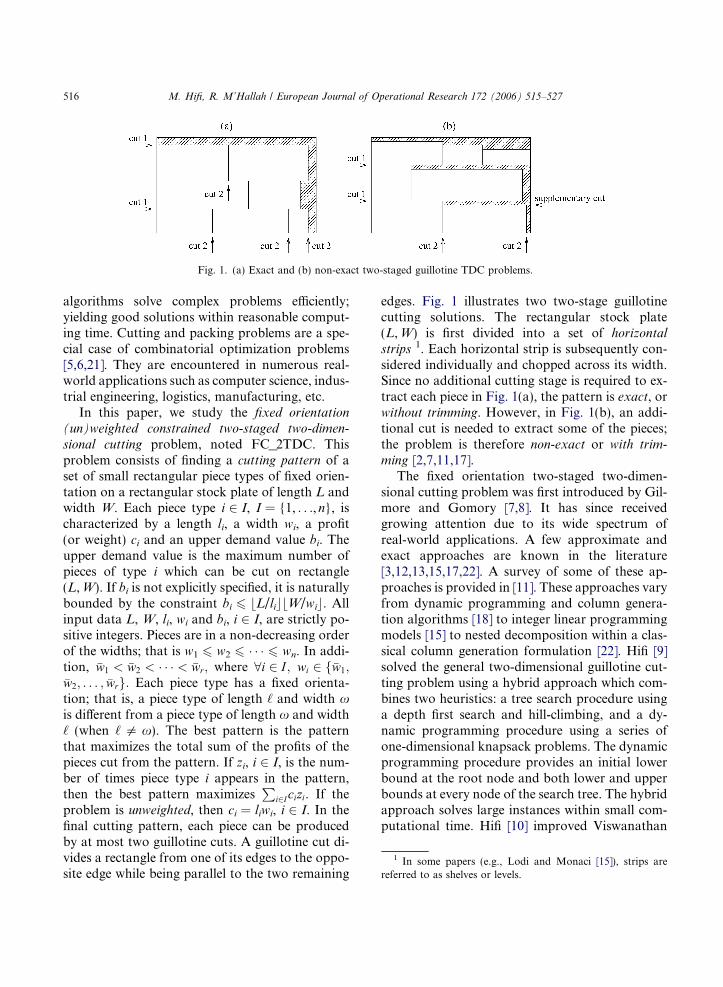
Fig. 1. (a) Exact and (b) non-exact two-staged guillotine TDC problems.

1 In some papers (e.g., Lodi and Monaci [15]), strips arereferred to as shelves or levels.

516 M. Hifi, R. M’Hallah / European Journal of Operational Research 172 (2006) 515–527

algorithms solve complex problems efficiently;yielding good solutions within reasonable comput-ing time. Cutting and packing problems are a spe-cial case of combinatorial optimization problems[5,6,21]. They are encountered in numerous real-world applications such as computer science, indus-trial engineering, logistics, manufacturing, etc.

In this paper, we study the fixed orientation

(un)weighted constrained two-staged two-dimen-

sional cutting problem, noted FC_2TDC. Thisproblem consists of finding a cutting pattern of aset of small rectangular piece types of fixed orien-tation on a rectangular stock plate of length L andwidth W. Each piece type i 2 I, I = {1, . . ., n}, ischaracterized by a length li, a width wi, a profit(or weight) ci and an upper demand value bi. Theupper demand value is the maximum number ofpieces of type i which can be cut on rectangle(L, W). If bi is not explicitly specified, it is naturallybounded by the constraint bi 6 bL/licbW/wic. Allinput data L, W, li, wi and bi, i 2 I, are strictly po-sitive integers. Pieces are in a non-decreasing orderof the widths; that is w1 6 w2 6 � � � 6 wn. In addi-tion, �w1 < �w2 < � � � < �wr; where 8i 2 I ; wi 2 f�w1;�w2; . . . ; �wrg: Each piece type has a fixed orienta-tion; that is, a piece type of length ‘ and width xis different from a piece type of length x and width‘ (when ‘ 5 x). The best pattern is the patternthat maximizes the total sum of the profits of thepieces cut from the pattern. If zi, i 2 I, is the num-ber of times piece type i appears in the pattern,then the best pattern maximizes

Pi2I cizi. If the

problem is unweighted, then ci = liwi, i 2 I. In thefinal cutting pattern, each piece can be producedby at most two guillotine cuts. A guillotine cut di-vides a rectangle from one of its edges to the oppo-site edge while being parallel to the two remaining

edges. Fig. 1 illustrates two two-stage guillotinecutting solutions. The rectangular stock plate(L, W) is first divided into a set of horizontal

strips 1. Each horizontal strip is subsequently con-sidered individually and chopped across its width.Since no additional cutting stage is required to ex-tract each piece in Fig. 1(a), the pattern is exact, orwithout trimming. However, in Fig. 1(b), an addi-tional cut is needed to extract some of the pieces;the problem is therefore non-exact or with trim-

ming [2,7,11,17].The fixed orientation two-staged two-dimen-

sional cutting problem was first introduced by Gil-more and Gomory [7,8]. It has since receivedgrowing attention due to its wide spectrum ofreal-world applications. A few approximate andexact approaches are known in the literature[3,12,13,15,17,22]. A survey of some of these ap-proaches is provided in [11]. These approaches varyfrom dynamic programming and column genera-tion algorithms [18] to integer linear programmingmodels [15] to nested decomposition within a clas-sical column generation formulation [22]. Hifi [9]solved the general two-dimensional guillotine cut-ting problem using a hybrid approach which com-bines two heuristics: a tree search procedure usinga depth first search and hill-climbing, and a dy-namic programming procedure using a series ofone-dimensional knapsack problems. The dynamicprogramming procedure provides an initial lowerbound at the root node and both lower and upperbounds at every node of the search tree. The hybridapproach solves large instances within small com-putational time. Hifi [10] improved Viswanathan

M. Hifi, R. M’Hallah / European Journal of Operational Research 172 (2006) 515–527 517

and Bagchi�s [23] exact algorithm for the con-strained guillotine two-dimensional cutting prob-lem. He introduced one-dimensional boundedknapsack problems in the original algorithm.These problems, solved by taking advantage ofthe properties of dynamic programming, yieldedgood lower and upper bounds that significantlycut branching. Using a similar strategy, Hifi andRoucairol [13] proposed both an approximateand an exact algorithm for the FC_2TDC.

In this paper, we solve the FC_2TDC problemusing several approximate algorithms. These algo-rithms start by generating strips, filling them withpieces, and subsequently searching for the ‘‘best’’combination of these strips. The best combinationis one that maximizes the sum of the profits of thepieces included in the rectangle (L, W) while notexceeding the demand of each piece type.

This paper is organized as follows. In Section 2,we summarize previous approximate algorithmsthat generate strips and combine them [9,13] andexplain how to adapt them to the FC_2TDC prob-lem. In Section 3, we improve the previous approx-imate algorithms and provide a better method forcombining strips. In Section 4, we present a newheuristic algorithm that combines a discretizationpoints procedure and hill-climbing strategies. InSection 5, we test the performance of the proposedversions of the approach on a set of small, mediumand large sized benchmark problems. Finally, inSection 6, we summarize the present work.

2. Strip generation algorithms

Strip generation algorithms (SGA) proceed intwo steps. First, they construct a set of strips. Sec-ond, they search for a good combination of someof those generated strips. A strip (a,b), with0 < a 6 L and 0 < b 6 W, is obtained by applyinga guillotine cut to the rectangle (L, W). If no tech-nological constraint applies to the problem, thefirst guillotine cut can be either horizontal or ver-tical. If the first cut is horizontal, then the strip isa horizontal strip (L,b). If the first cut is vertical,then the strip is a vertical strip (a, W). Withoutany loss of generality, we assume throughout thepaper that the first cut is horizontal.

There are two types of strips: uniform and gen-eral. A strip is uniform if it contains different piecetypes of identical width while a strip is general if itcontains piece types of different widths.

2.1. Uniform strips

2.1.1. SGA

The first step of SGA consists of generating asingle uniform strip ðL; �wjÞ for each distinct width�wj; j 2 J ; J ¼ f1; . . . ; rg. The strip ðL; �wjÞ is filledaccording to the optimal solution of the singleBounded Knapsack problem:

ðBKL;�wjÞ

f�wjðLÞ ¼ maxP

i2S�wj

cixij;

subject toP

i2S�wj

lixij 6 L;

xij 6 bi; xij 2 N; i 2 S �wj ;

8>>>><>>>>:

where S �wj ¼ Su�wj

, xij is the number of times piecetype i appears in the strip ðL; �wjÞ, and f�wjðLÞ theresulting profit. Su

�wj¼ fi 2 I ; wi ¼ �wjg; that is,

Su�wj

is the set of piece types whose width equals�wj. Since strip ðL; �wrÞ is the widest strip, solvingðBKL;�wrÞ using dynamic programming [14,16] yieldsthe optimal solution to every ðBKL;�wjÞ; j 2 J .

The second step of SGA determines the numberof occurrences yj of each of the uniform stripsðL; �wjÞ; j 2 J , in the rectangle (L, W) as to maxi-mize the total profit while not exceeding the de-mand bi of each piece type i 2 I. Indeed, theoptimal cutting pattern is filled according to theoptimal solution of the single bounded knapsackproblem:

ðBKPL;W Þ

gLðW Þ ¼ maxPj2J

f�wjðLÞyj;

subject toPj2J

�wjyj 6 W ;

yj 6 aj; yj 2 N; j 2 J :

8>>><>>>:

The number of occurrences yj of strip ðL; �wjÞ, j 2 J,in (L, W), has an upper bound

aj¼minW�wj

� �;min

i2S�wj

bi

xij

� �with xij > 0

� �( ): ð1Þ


2.1.2. A better SGA

The approximate solution of SGA can furtherbe improved. Indeed, the current solution ofSGA includes yj duplicates of each stripðL; �wjÞ; j 2 J ; where each uniform strip has beenobtained by solving ðBKL;�wjÞ. As yj is integer, thedemand for piece type i 2 S �wj may not be totallyexhausted; i.e., bi � xijyj; i 2 S �wj , could be strictlypositive. To improve the current solution ofSGA, we create, for each width �wj; j 2 J , in addi-tion to each uniform strip ðL; �wjÞ, Nj uniform strips

of length L and width �wj. These strips are toexhaust the total demand of the piece typesi 2 S �wj . Therefore, we will have a total ofN ¼ r þ

Pj2J N j strips: the original r strips

obtained by solving ðBKL;�wjÞ, j 2 J, and N � r

new strips obtained by solving additionalðBKL;�wjÞ; j 2 J , with bi set to bNj

i ; the residual de-mand for piece type i; i 2 S �wj after solving Nj + 1times ðBKL;�wjÞ. In fact, for every distinct width�wj, j 2 J, there will be Nj + 1 uniform strips thatare eligible to enter the rectangle (L, W). The algo-rithm proceeds as follows.

1. Step 1

Solve ðBKL;�wjÞ; j 2 J .Set Nj = 0, j 2 J.

Set b0i ¼ bi; i 2 I , and a0

j ¼ aj; j 2 J , whereaj is given by Eq (1).Set x0

ij ¼ xij; i 2 I ; j 2 J .

Set f 0�wjðLÞ ¼ f�wjðLÞ;

Set b1i ¼ b0

i � a0j x0

ij; 8i 2 S �wj ; j 2 J :2. Step 2

For j = 1, . . ., r,
Update S �wj ; i.e., S �wj ¼ fi 2 I ;wi ¼ �wj;
bNjþ1i > 0g.

If S �wj 6¼ ;,set Nj = Nj + 1;solve ðBKL;�wjÞ with bi ¼ bNj

i ;

set f Nj�wjðLÞ ¼ f�wjðLÞ;

set xNjij ¼ xij; i 2 I ; j 2 J ;

set aNjj ¼ mini2S�wj

jb

Njixij

k; xij > 0

� �; and

set bNjþ1i ¼ bNj

i � aNjj xij 8i 2 S �wj .

Step 3

If $i 2 I such that bNjþ1i > 0, go to Step 2.

Set N ¼ r þPr

j¼1N j:

Once we have generated the N uniform strips, wefill the rectangle (L, W) according to the optimalsolution of the following single bounded knapsackproblem:

ðBKP0L;W Þ

g0LðW Þ¼maxPj2J

PNj

m¼0

f m�wjðLÞym

j ;

subject toPj2J

PNj

m¼0

�wjymj 6W ;

ymj 6 am

j ; ymj 2N;

j2 J ; m¼ 0; . . . ;Nj;

8>>>>>>>><>>>>>>>>:

where ymj is the number of occurrences of the mth

type of the uniform strip ðL; �wjÞ, m = 0, . . ., Nj,j 2 J.

2.2. General strips

We generate a single general strip of length L

and width �wj for each distinct width �wj; j 2 J .To generate these general strips, we use the sameknapsack problems ðBKL;�wjÞ; j 2 J , with theexception that the pieces included in the strip donot necessarily have equal widths. In fact,S �wj ¼ Sg

�wj, where Sg

�wj¼ fi 2 I ;wi 6 �wjg; that is,

Sg�wj

is the set of pieces belonging to the general strip

ðL; �wjÞ. Let xNjþ1ij ; i 2 I , denote the optimal solu-

tion value of ðBKL;�wjÞ; j 2 J , and let f Njþ1�wjðLÞ de-

note its corresponding objective function value.A general feasible cutting pattern combines

strips from the set of N uniform and r generalstrips. The optimal cutting pattern is the solutionto the integer linear program:

ðIP L;W Þ

hLðW Þ ¼ maxPj2J

PNjþ1

m¼0

f m�wjðLÞym

j ;

subject toPj2J

PNjþ1

m¼0

�wjymj 6 W ;

Pj2J

PNjþ1

m¼0

xmijy

mj 6 bi; i 2 I ;

ymj 2 N; j 2 J ;

m ¼ 0; . . . ;Nj þ 1;

8>>>>>>>>>>>>>><>>>>>>>>>>>>>>:

where ymj is the number of occurrences of the mth

type of strip ðL; �wjÞ in the stock rectangle (L, W),and xm

ij denotes the number of occurrences of the


ith piece in that strip. We solve (IPL,W), which isNP-hard, using an approximate algorithm,adapted from the greedy algorithm of [10], andsummarized below.

2.2.1. The greedy algorithm

1. Set bui ¼ bi for i 2 I, where bu

i is the currentunsatisfied demand of piece type i.

2. Select, among the N + r available strips, thestrip ðL; �wkÞ having the highest profit to usageratio; that is

f�wk ðLÞPi2S�wk

xik¼ max

j¼1;...;rm¼0;...;Njþ1

f mwjðLÞP

i2S�wjxm

ij

( ):

3. Position strip ðL; �wkÞ on rectangle (L, W).4. For every piece type i in strip ðL; �wkÞ, if bu

i < xik,then reduce the number of pieces of type i instrip ðL; �wkÞ to bu

i , and set xik ¼ bui .

5. Update the current demand of every piece typei in strip ðL; �wkÞ; that is bu

i ¼ bui � xik; i 2 S �wk .

Remove any piece type with a null demandfrom further consideration.

6. Fill the remaining region of strip ðL; �wkÞ usingthe filling procedure (FP) detailed in Section2.2.2.

7. Update the remaining width of rectangle (L, W);that is W ¼ W � �wk.

8. If there exists a piece type i 2 I such that bui > 0,

and wi 6 W, go to Step 2; else stop.

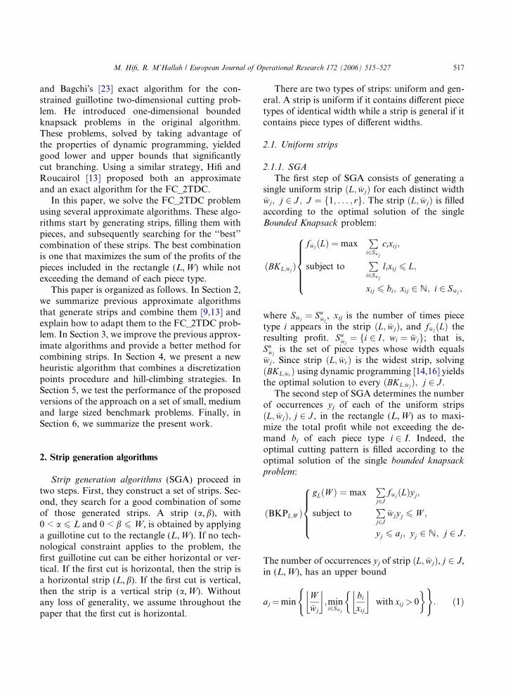
2.2.2. The filling procedure (FP)The filling procedure FP (used in Step 6 of the

greedy algorithm) fills strips using piece typeswhose demands are strictly positive. To illustrate

Fig. 2. Illustration of the second p

FP, we consider the general strip (L, y) of Fig.2(a). First, Step 4 of the greedy algorithm removesthe pieces which violate the demand constraints asshown in Fig. 2(b); thus, it creates holes into thestrip. These holes are the regions 1 and 2 of Fig.2(c). Second, FP concatenates the created holesby shifting the positioned pieces to the left. Theconcatenated hole is region 3 of Fig. 2(d). Third,FP fills this generated region or substrip of dimen-sions (L � L 0, y) by solving the following knap-sack problem:

maxXi2Sy

cizi jXi2Sy

lizi 6 L� L0; zi 6 bui ;

(

zi 2 N; i 2 Sy

);

where Sy :¼ {s 2 Ij(ls, ws) 6 (L�L 0, y)}. That is,FP is restricted to a sequential horizontal fillingas shown in Fig. 2(d).

FP solves a series of knapsack problems using,for each problem, either an approximate or an ex-act procedure. Of course, solving the knapsackproblems using an exact procedure is more timeconsuming than solving it using an approximateone. Unless specifically stated, the knapsack prob-lems are solved using an approximate algorithm.

3. An extended strip generation approach (ESGA)

The main idea of the algorithm consists individing the rectangle (L, W) into two subrectan-gles (L,b) and (L, W � b), where the choice ofthe value of b will be explained later. The first sub-rectangle (L,b) is generated and filled using SGAwhile the second subrectangle (L, W � b) is filledusing an alternative procedure.

hase of the greedy approach.


Indeed, ESGA starts by creating strips of lengthL. It then selects among these strips the best stripsthat fill the stock rectangle (L, W). As the selectionprocess is not straightforward, ESGA—based on adiscretization points procedure—deals with a finitenumber of subrectangles. These subrectangles are inturn filled with horizontal strips. To speed up the‘‘filling process’’, we introduce an upper boundthat eliminates unnecessary branchings.

3.1. The discretization points procedure

The discretization points procedure limits thesearch to a finite number of (sub)rectangles whichcan potentially provide good solutions. To dealwith a finite number of cuts, we discretize thewidth of each (sub)rectangle as Christofides andWhitlock [4] did for the unstaged TDC problem.For a subrectangle (L,b), the set of linear combi-nations of the widths is

QðL;bÞ ¼ y j y ¼Xi2Sb

wizi 6 b;

8<:

zi 6 min bi;

�Lli

��bwi

�� ; zi 2 N

9=;;

where Sb = {i 2 Ijwi 6 b}.

3.2. An upper bound for a normalized subrectangle

An upper bound allows us to avoid filling somesubrectangles. Let b 2 QðL;W Þ be a valid cut and let(L,b) be the current resulting subrectangle with(L0,b0) its normalized subrectangle such that

L0 ¼ maxx2PðL;bÞ

fxg and b0 ¼ maxy2QðL;bÞ

fyg;

where

PðL;bÞ ¼�

x j x ¼X

i2Ilizi 6 L; wi 6 b;

zi 6 min bi;

�Lli

��bwi

�� ; zi 2 N

�:

An upper bound UðL;bÞ for the profit is obtainedby filling (L0,b0) according to the optimal solutionof the knapsack problem KPU. That is,

UðL;bÞ ¼ maxXj2J

f�wjðLÞzj jXj2J

�wjzj 6 b;

(

zj 2 N; j ¼ 1 2 J

);

where f�wjðLÞ is the profit generated by the generalstrip ðL; �wjÞ while zj is the number of occurrencesof that strip in (L,b). To solve KPU, we apply adynamic programming procedure that initiallyconstructs all upper bounds corresponding to allpossible subrectangles (L, y) with 0 6 y 6 W.Next, we consider a b-cut and suppose that (L,b)represents the resulting normalized subrectangle.We, then, discard the normalized subrectangle(L 0,b 0) of (L, W � b) if

LowerðL;bÞ þUðL0 ;b0Þ 6 BestðL;W Þ;

where Best(L,W) denotes the current best solutionvalue of (L, W) and Lower(L,b) the best feasiblesolution value obtained for (L,b).

3.3. Algorithm

Fig. 3 describes the main steps of ESGA. Thealgorithm uses two main procedures:

1. procedure Initialization[] which gener-ates both uniform and general strips; and

2. procedure Construct[] which reduces thenumber of (sub)rectangles capable of providingbetter solutions to a finite number.

ESGA uses a combination of (uniform or gen-eral) strips and of strips generated by FP. Evi-dently, other combinations could be considered,for example, solving exactly each knapsack prob-lem when FP is applied. However, our limitedcomputational results showed that the strategycurrently used by ESGA produced good qualityresults within reasonable computing times.

4. Hill-climbing ESGA

Hill-climbing (HC) is a simple but popular heu-ristic strategy that is based upon local search

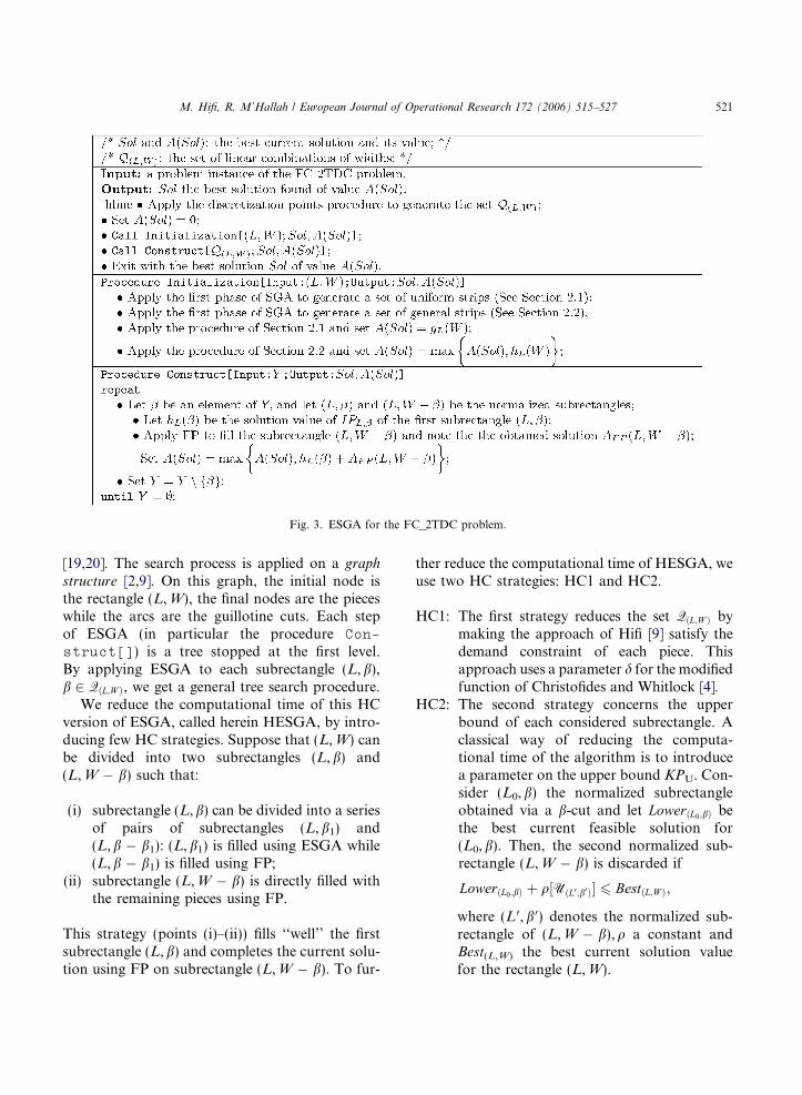
Fig. 3. ESGA for the FC_2TDC problem.


[19,20]. The search process is applied on a graph

structure [2,9]. On this graph, the initial node isthe rectangle (L, W), the final nodes are the pieceswhile the arcs are the guillotine cuts. Each stepof ESGA (in particular the procedure Con-

struct[]) is a tree stopped at the first level.By applying ESGA to each subrectangle (L,b),b 2 QðL;W Þ, we get a general tree search procedure.

We reduce the computational time of this HCversion of ESGA, called herein HESGA, by intro-ducing few HC strategies. Suppose that (L, W) canbe divided into two subrectangles (L,b) and(L, W � b) such that:

(i) subrectangle (L,b) can be divided into a seriesof pairs of subrectangles (L,b1) and(L,b � b1): (L,b1) is filled using ESGA while(L,b � b1) is filled using FP;

(ii) subrectangle (L, W � b) is directly filled withthe remaining pieces using FP.

This strategy (points (i)–(ii)) fills ‘‘well’’ the firstsubrectangle (L,b) and completes the current solu-tion using FP on subrectangle (L, W � b). To fur-

ther reduce the computational time of HESGA, weuse two HC strategies: HC1 and HC2.

HC1: The first strategy reduces the set QðL;W Þ bymaking the approach of Hifi [9] satisfy thedemand constraint of each piece. Thisapproach uses a parameter d for the modifiedfunction of Christofides and Whitlock [4].

HC2: The second strategy concerns the upperbound of each considered subrectangle. Aclassical way of reducing the computa-tional time of the algorithm is to introducea parameter on the upper bound KPU. Con-sider (L0,b) the normalized subrectangleobtained via a b-cut and let LowerðL0;bÞ bethe best current feasible solution for(L0,b). Then, the second normalized sub-rectangle (L, W � b) is discarded if

LowerðL0;bÞ þ q½UðL0;b0Þ� 6 BestðL;W Þ;

where (L 0,b 0) denotes the normalized sub-rectangle of (L, W � b), q a constant andBest(L,W) the best current solution valuefor the rectangle (L, W).

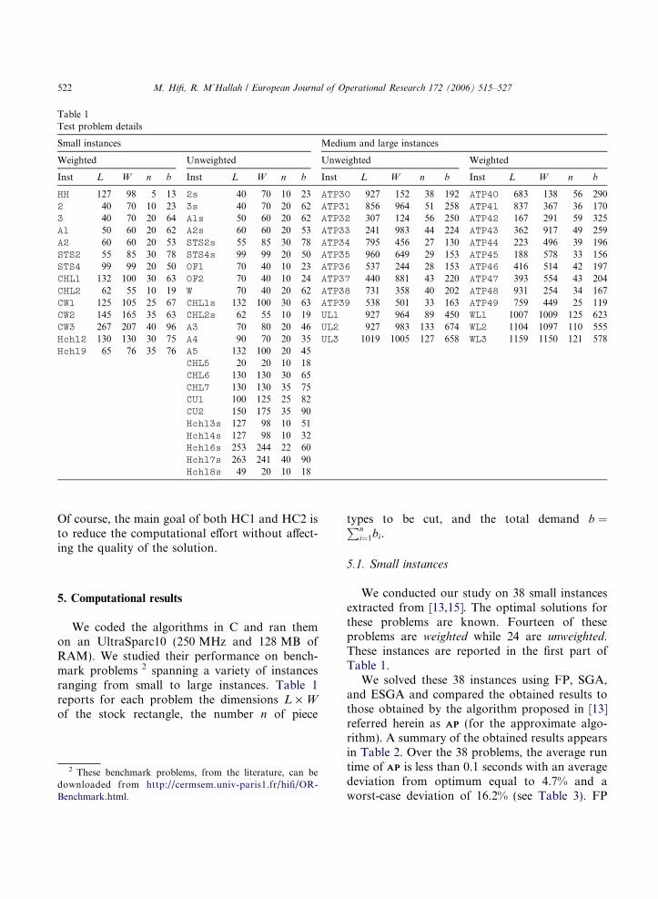
Table 1Test problem details

Small instances Medium and large instances

Weighted Unweighted Unweighted Weighted

Inst L W n b Inst L W n b Inst L W n b Inst L W n b

HH 127 98 5 13 2s 40 70 10 23 ATP30 927 152 38 192 ATP40 683 138 56 2902 40 70 10 23 3s 40 70 20 62 ATP31 856 964 51 258 ATP41 837 367 36 1703 40 70 20 64 A1s 50 60 20 62 ATP32 307 124 56 250 ATP42 167 291 59 325A1 50 60 20 62 A2s 60 60 20 53 ATP33 241 983 44 224 ATP43 362 917 49 259A2 60 60 20 53 STS2s 55 85 30 78 ATP34 795 456 27 130 ATP44 223 496 39 196STS2 55 85 30 78 STS4s 99 99 20 50 ATP35 960 649 29 153 ATP45 188 578 33 156STS4 99 99 20 50 OF1 70 40 10 23 ATP36 537 244 28 153 ATP46 416 514 42 197CHL1 132 100 30 63 OF2 70 40 10 24 ATP37 440 881 43 220 ATP47 393 554 43 204CHL2 62 55 10 19 W 70 40 20 62 ATP38 731 358 40 202 ATP48 931 254 34 167CW1 125 105 25 67 CHL1s 132 100 30 63 ATP39 538 501 33 163 ATP49 759 449 25 119CW2 145 165 35 63 CHL2s 62 55 10 19 UL1 927 964 89 450 WL1 1007 1009 125 623CW3 267 207 40 96 A3 70 80 20 46 UL2 927 983 133 674 WL2 1104 1097 110 555Hchl2 130 130 30 75 A4 90 70 20 35 UL3 1019 1005 127 658 WL3 1159 1150 121 578Hchl9 65 76 35 76 A5 132 100 20 45

CHL5 20 20 10 18CHL6 130 130 30 65CHL7 130 130 35 75CU1 100 125 25 82CU2 150 175 35 90Hchl3s 127 98 10 51Hchl4s 127 98 10 32Hchl6s 253 244 22 60Hchl7s 263 241 40 90Hchl8s 49 20 10 18


Of course, the main goal of both HC1 and HC2 isto reduce the computational effort without affect-ing the quality of the solution.

5. Computational results

We coded the algorithms in C and ran themon an UltraSparc10 (250 MHz and 128 MB ofRAM). We studied their performance on bench-mark problems 2 spanning a variety of instancesranging from small to large instances. Table 1reports for each problem the dimensions L · W

of the stock rectangle, the number n of piece

2 These benchmark problems, from the literature, can bedownloaded from http://cermsem.univ-paris1.fr/hifi/OR-Benchmark.html.

types to be cut, and the total demand b ¼Pni¼1bi.

5.1. Small instances

We conducted our study on 38 small instancesextracted from [13,15]. The optimal solutions forthese problems are known. Fourteen of theseproblems are weighted while 24 are unweighted.These instances are reported in the first part ofTable 1.

We solved these 38 instances using FP, SGA,and ESGA and compared the obtained results tothose obtained by the algorithm proposed in [13]referred herein as APAP (for the approximate algo-rithm). A summary of the obtained results appearsin Table 2. Over the 38 problems, the average runtime of APAP is less than 0.1 seconds with an averagedeviation from optimum equal to 4.7% and aworst-case deviation of 16.2% (see Table 3). FP

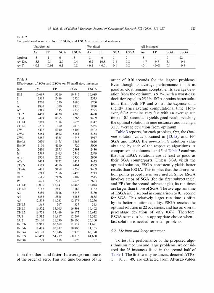
http://cermsem.univ-paris1.fr/hifi/OR-Benchmark.html

http://cermsem.univ-paris1.fr/hifi/OR-Benchmark.html

Table 2Computational results of APP, FP, SGA, and ESGA on small sized instances

Unweighted Weighted All instances

APP FP SGA ESGA APP FP SGA ESGA APP FP SGA ESGA

Optima 5 1 6 15 3 0 3 7 8 1 9 22Av Dev 3.8 9.1 2.7 0.4 6.2 10.8 3.8 0.8 4.7 9.7 3.1 0.6Av T <0.1 <0.01 0.1 0.8 <0.1 <0.01 0.1 0.8 <0.1 <0.01 0.1 0.8

Table 3Effectiveness of SGA and ESGA on 38 small sized instances

Inst Opt FP SGA ESGA

HH 10,689 9516 10,545 10,6892 2535 2489 2520 25353 1720 1550 1680 1700A1 1820 1700 1820 1820A2 2315 1735 2135 2295STS2 4450 4220 4280 4420STS4 9409 8965 9263 9409CHL1 8360 7314 7695 8347CHL2 2235 1960 2076 2235CW1 6402 6040 6402 6402CW2 5354 4562 5354 5354CW3 5287 4335 4748 4947Hchl2 9630 8475 9366 9616Hchl9 5100 4510 4720 50002s 2430 2375 2393 24303s 2599 2405 2546 2599A1s 2950 2322 2950 2950A2s 3423 3372 3423 3423STS2s 4569 4356 4464 4569STS4s 9481 9158 9258 9409OF1 2713 2356 2496 2713OF2 2515 2126 2307 2515W 2623 2277 2623 2623CHL1s 13,036 12,041 12,448 13,014CHL2s 3162 2891 3162 3162A3 5380 5116 5348 5380A4 5885 5885 5885 5885A5 12,553 11,263 12,276 12,276CHL5 363 307 337 363CHL6 16,572 15,005 16,398 16,402CHL7 16,728 15,469 16,172 16,632CU1 12,312 11,917 12,269 12,312CU2 26,100 21,390 26,100 26,100Hchl3s 11,961 10,669 11,517 11,691Hchl4s 11,408 10,032 10,806 11,165Hchl6s 60,170 55,046 57,926 60,170Hchl7s 62,459 54,219 60,713 61,660Hchl8s 729 678 692 727


is on the other hand faster. Its average run time isof the order of zero. This run time becomes of the

order of 0.01 seconds for the largest problems.Even though its average performance is not asgood as APAP, it remains acceptable. Its average devi-ation from the optimum is 9.7%, with a worst-casedeviation equal to 25.1%. SGA obtains better solu-tions than both FP and APAP at the expense of aslightly larger average computational time. How-ever, SGA remains very fast with an average runtime of 0.1 seconds. It yields good results reachingthe optimal solution in nine instances and having a3.1% average deviation from optimum.

Table 3 reports, for each problem, Opt, the Opti-

mal solution value obtained in [13,15], and FP,SGA and ESGA the approximate solution valueobtained by each of the respective algorithms. Acomparison of columns 4 and 5 of Table 3 confirmsthat the ESGA solutions are at least as good astheir SGA counterparts. Unless SGA yields theoptimal solution, ESGA consistently yields betterresults than ESGA. This implies that the discretiza-tion points procedure is very useful. Since ESGAinvolves steps of SGA (for the first subrectangle)and FP (for the second subrectangle), its run timesare larger than those of SGA. The average run timeof ESGA is 0.8 second in comparison to 0.1 secondfor SGA. This relatively larger run time is offsetby the better solutions quality. ESGA reaches theoptimal solution in 22 occasions, and has an overallpercentage deviation of only 0.6%. Therefore,ESGA seems to be an appropriate choice when afast solution is needed for small problems.

5.2. Medium and large instances

To test the performance of the proposed algo-rithms on medium and large problems, we consid-ered the 26 instances listed in the second half ofTable 1. The first twenty instances, denoted ATPx,x = 30, . . ., 49, are extracted from Alvarez-Valdes

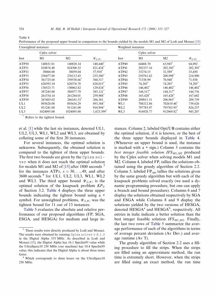
Table 4Performance of the proposed upper bound in comparison to the bounds yielded by the models M1 and M2 of Lodi and Monaci [15]

Unweighted instances Weighted instances

Cplex solver Cplex solver

Inst M1 M2 UðL;W Þ Inst M1 M2 UðL;W Þ

ATP30 140831.81 140828.14 140,440* ATP40 64468.70 63,945* 64,092ATP31 824876.40 824300.52 821,424* ATP41 202337.16 202,305* 202,305*

ATP32 38068.00 38059.04 37,910* ATP42 33274.15 32,589* 33,450ATP33 236477.88 236113.43 235,580* ATP43 210761.62 208,998* 214,900ATP34 361725.68 359538.66* 360,517 ATP44 71338.99 70,940* 71,938ATP35 620593.54 620376.78 620,015* ATP45 74,205* 74,205* 74,205*

ATP36 130523.71 130062.82 129,824* ATP46 146,402* 146,402* 146,402*

ATP37 387245.00 386977.79 385,121* ATP47 144,317* 144,317* 144,736ATP38 261534.14 261284.01 259,908* ATP48 165,428* 165,428* 167,602ATP39 267603.02 266161.53* 266,361 ATP49 209011.31 206,965* 209,759UL1 893628.00 893616.29 893,368* WL1 708212.86 702619.46* 739,626UL2 911241.00 911241.00 910,994* WL2 797783.97 793763.95* 826,257UL3 1024095.00 1024095.00 1,023,599* WL3 916928.77 912969.82* 945,207

* Refers to the tightest bound.


et al. [1] while the last six instances, denoted UL1,UL2, UL3, WL1, WL2 and WL3, are obtained bycollating some of the first 20 instances.

For several instances, the optimal solution isunknown. Subsequently, the obtained solution iscompared to the tightest of three upper bounds.The first two bounds are given by the Cplex sol-ver when it does not reach the optimal solutionfor models M1 and M2 of [15] after 1800 seconds 3

for the instances ATPx, x = 30, . . ., 49, and after3600 seconds 4 for UL1, UL2, UL3, WL1, WL2and WL3. The third upper bound UðL;W Þ is theoptimal solution of the knapsack problem KPU

of Section 3.2. Table 4 displays the three upperbounds indicating the tightest bound using a *symbol. For unweighted problems, UðL;W Þ was thetightest bound for 11 out of 13 instances.

Table 5 evaluates the absolute and relative per-formance of our proposed algorithms (FP, SGA,ESGA, and HESGA) for medium and large in-

3 These results were directly produced by Lodi and Monaci.The results were obtained by running Cplex solver v.8.1.0in the Digital Alpha 533 MHz. As described in Lodi andMonaci [15], the Digital Alpha has 16.1 SpecInt95 value whilethe UltraSparc10 250 MHz (our machine) has 10.4 SpecInt95value; this indicates that the Digital Alpha is about three timesfaster.

4 Which corresponds to three hours on the UltraSparc10250 MHz.

stances. Column 2, labeled Opt/UB contains eitherthe optimal solution, if it is known, or the best ofthe three upper bounds displayed in Table 4.(Whenever an upper bound is used, the instanceis marked with a * sign.) Column 3 contains thebest integer feasible solution IFSM1,M2 producedby the Cplex solver when solving models M1 andM2. Column 4, labeled FP, tallies the solutions ob-tained using the greedy algorithm of Section 2.2.Column 5, labeled FPopt tallies the solutions givenby the same greedy algorithm but with each of theknapsack problems solved exactly (we used a dy-namic programming procedure, but one can applya branch and bound procedure). Columns 6 and 7display the solutions obtained respectively by SGAand ESGA while Columns 8 and 9 display thesolutions yielded by the two versions of HESGA,denoted HESGAa and HESGAb, respectively. Allentries in italic indicate a better solution than thebest integer feasible solution IFSM1,M2. Finally,the last two rows of Table 5 summarize the aver-age performance of each of the algorithms in termsof average percent deviation (Av Dev.) and aver-age runtime (Av T).

The greedy algorithm of Section 2.2 uses a fill-ing procedure to fill the strips. When the stripsare filled using an approximate method, the runtime is extremely short. However, when the stripsare filled using an exact method, the run time

Table 5Effectiveness of the strip generation algorithms compared to the Cplex solver

Inst Opt/UB Cplex solver Strip Generation Algorithms

IFSM1,M2 FP FPopt SGA ESGA HESGAa HESGAb

ATP30 140440* 139,239 132,533 132,698 139,900 140,168 140,168 140,168

ATP31 821,424* 818,364 788,839 801,009 814,608 816,834 818,512 820,260

ATP32 37,910* 37,344 37,028 37,028 37,455 37,880 37,880 37,880

ATP33 235,580 235,580 221,291 225,569 233,812 234,350 234,564 235,580ATP34 359538.66* 356,159 335,496 337,232 343,222 354,998 356,159 356,159ATP35 620,015 610,547 583,582 589,498 609,313 613,784 613,784 614,429

ATP36 129,824* 129,262 127,826 128,714 128,714 129,262 129,262 129,262ATP37 385,121* 381,766 370,308 376,040 381,103 382,612 382,910 384,478

ATP38 259,908 259,070 249,207 251,857 254,798 256,911 258,221 259,070ATP39 266161.53* 266,135 249,049 258,562 263,222 265,306 265,621 266,135ATP40 63,945 63,945 61,181 61,620 63,622 63,657 63,945 63,945ATP41 202,305 202,305 189,659 202,305 202,305 202,305 202,305 202,305ATP42 32,589 32,589 27,461 27,922 29,093 31,230 32,589 32,589ATP43 208,998 208,998 191,176 185,979 206,494 208,571 208,571 208,998ATP44 70,940 70,940 69,738 70,646 70,176 70,242 70,678 70,940ATP45 74,205 74,205 74,205 74,205 74,205 74,205 74,205 74,205ATP46 146,402 146,402 126,760 125,986 141,921 146,402 146,402 146,402ATP47 144,317 144,317 136,044 137,762 141,425 143,458 143,458 144,317ATP48 165,428 165,428 154,805 154,967 154,805 159,357 162,032 165,428ATP49 206,965 206,965 169,211 169,211 196,745 200,897 204,574 206,965UL1 893,368* 876,682 868,921 877,403 885,909 886,037 886,879 887,099

UL2 910,994* 900,923 884,523 890,421 902,711 904,579 905,985 906,237

UL3 1,023,599* 1,009,031 985,858 988,398 1,010,845 1,013,758 1,013,792 1,017,575

WL1 702619.46* 687,786 539,714 541,221 661,473 682,034 688,413 688,840

WL2 793763.95* 778,028 576,408 581,954 721,420 778,086 779,359 782,566

WL3 912969.82* 897,373 767,892 773,198 882,195 894,160 897,651 899,890

Av Dev 1.05 9.49 8.72 2.89 1.27 0.88 0.63Av T – 0.15 14.75 7.96 15.10 134.80 296.96


increases while the solution quality improves. Tohave a fair comparison of the two filling ap-proaches, we maintained the same ordering ofthe widths (of course, other orders can be usedand may produce better solutions). For the usedorder, FP is still very fast even for medium andlarge instances; its average run time is 0.15 sec-onds. It still yields reasonably good results withan average percent deviation of 9.49%. Evidently,FPopt produces better solutions with an averagepercent deviation of 8.72% but at the expense ofa larger computational time. The average run timeof FPopt is 14.75 seconds. The percent improve-ment brought by filling the strips exactly doesnot warrant the larger increase in run time. Inaddition, given that the greedy algorithm is to beused several times in the proposed algorithmsand in order to maintain the run time of these

algorithms acceptable, we opted—within the gree-dy algorithm—to fill the knapsack problems usingFP.

SGA (Column 6 of Table 5) produces bettersolutions than either FP or FPopt: SGA�s percentdeviation is 2.89% in comparison to 9.49%, and8.72% for FP and FPopt, respectively. SGA per-forms better than FPopt not only in terms of solu-tion quality but also in terms of run time. SGAuses only about half the run time required by FPopt

with a factor of three improvement of the solutionquality. Most importantly, SGA produces bettersolutions than IFSM1,M2 for the three large un-weighted instances UL1, UL2, and UL3.

ESGA produces better solutions than FPopt

within an equivalent average run time. As ex-pected, ESGA further improves the solution qual-ity obtained by SGA; reducing the percent


deviation from optimum to 1.27%. Similarlyto SGA, ESGA produces better solutions thanIFSM1,M2 in four out of six large instances.

Columns 8 and 9 of Table 5, labeled HESGAa

and HESGAb, respectively, display the solutionsgiven by the two versions of HESGA. Recall thatthe implementation of HESGA involves the set upof two parameters: d and q corresponding respec-tively to strategies (HC1) and (HC2). While thesecond strategy (HC2) is identical in both versions,the first strategy is not. The first implementation ofHESGA, denoted HESGAa, uses the strategyHC1(a) while the second implementation, denotedHESGAb, uses the strategy HC1(b). The selectedstrategies proceed as follows.

HC1(a): Each step of the procedure Con-

struct[] creates, using a b-cut, twosubrectangles (L,b) and (L, W � b).For these b-cuts, we fix d = 2. WhenHESGA tries to improve the solutionon the first subrectangle (L,b), usingthe discretization points procedure, wereduce QðL;bÞ to {wi : wi 6 b}.

HC1(b): As in HC1(a), for the b-cuts, we fixd = 2. When the procedure tries to pro-duce a better solution on the first subrec-tangle (L,b), we extend the set of linearcombinations to QðL;bÞ by locally fixingd = 2; thus, more linear combinationsare considered, and better solutions canpotentially be reached.

HC2: Since the upper bound is generally verytight, we set q = 0.999, when a b-cut isto be made, and q = 0.99 when the b-cut has already been made (the discreti-zation points procedure is extended tothe first subrectangle (L,b)).

These strategies seem, among the different strate-gies we explored, to be a good compromise interms of solution quality and run time. It is clearthat applying HESGA without the hill-climbingstrategies would require very large computationaltimes.

The study of Table 5 shows that either imple-mentation of HESGA reaches better solutionsthan any of the other strip generation algorithms.

For the medium instances (APTx, x = 30, . . ., 49),HESGAa improves the solutions of 11 out of 20instances while HESGAb improves the solutionsof 14 out of 20 instances.

In addition, both HESGAa and HESGAb pro-duce better solutions than the Cplex solver

with average percent deviations of 0.88% and0.63% for HESGAa and HESGAb, and 1.05%for the Cplex solver.

To evaluate the performance of both versions ofHESGA relative to the performance of the Cplexsolver for the large instances UL1, UL2, UL3,WL1, WL2 and WL3, we proceeded as follows.We set the runtime limit of the Cplex Solver

to 3 hour, of HESGAa to 250 seconds and ofHESGAb to 500 seconds. For those six large in-stances, both HESGAa and HESGAb reach bettersolutions than IFSM1,M2. A comparison of the twoimplementations of HESGA reveals that HESGAb

reaches better solutions than HESGAa. Evidently,these improvements occur at the cost of a largercomputational time. However, the improvementof the solution quality warrants the additionalrun time.

In conclusion, either implementation ofHESGA yields near optimal solutions for mediumand large sized problems. In addition, for largeproblems, any of the strip generation algorithmsseems to be a plausible approach in particularfor unweighted problems.

Finally, it is noteworthy that if no technologicalconstraint requires the first cut to be horizontal,then the previous algorithms can be run twice:once with the first cut being horizontal and oncewith the first cut being vertical. The best of thetwo solutions is then adopted. When the first cutis vertical, the previous algorithms can be usedonce the dimensions of each piece type i 2 I andthe dimensions of the rectangular stock (L, W)are swapped from (li, wi) to (wi, li), and from(L, W) to (W, L), respectively.

6. Conclusion

In this paper, we considered the constrainedtwo-staged two-dimensional guillotine cuttingproblem. First, we proposed a strip generation


approach based on solving single bounded knap-sack problems. Second, we extended this approachand made it combine strips obtained using thestrip generation procedure and those obtainedusing a filling procedure. Third, we further im-proved this approach using hill-climbing strate-gies; making the algorithm better adapted tolarge problems. The experiments conducted on dif-ferent instances varying from small to large sizedinstances show that the algorithms produce goodsolutions within reasonable run times.

Acknowledgments

The authors thank the anonymous referees andthe Editor-in-Chief Roman Slowinski for theirhelpful comments which contributed to theimprovement of the contents of this paper. Theauthors thank also Andrea Lodi and MicheleMonaci for sending the results of the Cplex solverof the twenty six medium and large instances,using both models M1 and M2 developed in [15].

References

[1] R. Alvarez-Valdes, A. Parajon, J.M. Tamarit, A tabusearch algorithm for large-scale guillotine (un)constrainedtwo-dimensional cutting problems, Computers and Oper-ations Research 29 (2002) 925–947.

[2] M. Arenales, R. Morabito, An overview of and–or-graphapproaches to cutting and packing problems, DecisionMaking under Conditions of Uncertainty, ISBN 5-86911-161-7, 1997, pp. 207–224.

[3] J.E. Beasley, Algorithms for unconstrained two-dimen-sional guillotine cutting, Journal of the OperationalResearch Society 36 (1985) 297–306.

[4] N. Christofides, C. Whitlock, An algorithm for two-dimensional cutting problems, Operations Research 2(1977) 31–44.

[5] H. Dyckhoff, A typology of cutting and packing problems,European Journal of Operational Research 44 (1990) 145–159.

[6] H. Dyckhoff, G. Scheithauer, J. Terno, Cutting andpacking (C&P), in: M. Dell�Amico, F. Maffioli, S. Martello(Eds.), Annotated Bibliographies in Combinatorial Opti-mization, John Wiley & Sons, Chichester, 1997.

[7] P.C. Gilmore, R.E. Gomory, Multistage cutting problemsof two and more dimensions, Operations Research 13(1965) 94–119.

[8] P.C. Gilmore, R.E. Gomory, The theory and computationof knapsack functions, Operations Research 14 (1966)1045–1074.

[9] M. Hifi, The DH/KD algorithm: A hybrid approach forunconstrained two-dimensional cutting problems, Euro-pean Journal of Operational Research 97 (1997) 41–52.

[10] M. Hifi, An improvement of Viswanathan and Bagchi�s exactalgorithm for constrained two-dimensional cutting stock,Computers and Operations Research 24 (1997) 727–736.

[11] M. Hifi, Contribution a la resolution de quelques proble-mes difficiles de l�optimisation combinatoire, HabilitationThesis. PRiSM, Universite de Versailles St-Quentin enYvelines, 1999.

[12] M. Hifi, Exact algorithms for large-scale unconstrainedtwo and three staged cutting problems, ComputationalOptimization and Applications 18 (2001) 63–88.

[13] M. Hifi, C. Roucairol, Approximate and exact algorithmsfor constrained (un)weighted two-dimensional two-stagedcutting stock problems, Journal of Combinatorial Optimi-zation 5 (2001) 465–494.

[14] E.L. Lawler, Fast approximation algorithms for knapsackproblems, Mathematics of Operations Research 4 (1979)339–356.

[15] A. Lodi, M. Monaci, Integer linear programming modelsfor 2-staged two-dimensional knapsack problems, Mathe-matical Programming 94 (2003) 257–278.

[16] S. Martello, P. Toth, An exact algorithm for largeunbounded knapsack problems, Operations Research Let-ters 9 (1990) 15–20.

[17] R. Morabito, M. Arenales, Staged and constrained two-dimensional guillotine cutting problems: An and–or-graphapproach, European Journal of Operational Research 94(3) (1996) 548–560.

[18] R. Morabito, V. Garcia, The cutting stock problem inhardboard industry: A case study, Computers and Oper-ations Research 25 (1998) 469–485.

[19] J. Pearl, Heuristics: Intelligent Search Strategies for Com-puter Problem Solving, Addison-Wesley, Reading, MA,1984.

[20] E. Rich, Artificial Intelligence, McGraw-Hill, New York,1983.

[21] P.E. Sweeney, E.R. Paternoster, Cutting and packingproblems: A categorized applications-oriented researchbibliography, Journal of the Operational Research Society43 (1992) 691–706.

[22] F. Vanderbeck, A nested decomposition approach to a 3-stage 2-dimensional cutting stock problem, ManagementScience 47 (2001) 864–879.

[23] K.V. Viswanathan, A. Bagchi, A best first search methodfor constrained two-dimensional cutting stock problems,Operations Research 41 (1993) 768–776.

strip generation algorithms for constrained two-dimensional two-staged cutting problems

Documents