strengthening and streamlining bank capital regulation
TRANSCRIPT

479
ROBIN GREENWOOD JEREMY C. STEINHarvard Business School Harvard University
SAMUEL G. HANSON ADI SUNDERAMHarvard Business School Harvard Business School
Strengthening and Streamlining Bank Capital Regulation
ABSTRACT We propose three core principles that should inform the design of bank capital regulation. First, whenever possible, multiple constraints on the minimum level of equity capital should be consolidated into a single constraint. This helps to avoid a distortionary situation where different constraints bind for different banks performing the same activity. Second, the best way to deal with the inevitable gaming of any set of ex ante capital rules is not to propose further rules, but rather to allow the regulator sufficient flexibility to address unforeseen contingencies ex post. Third, though a regulatory framework that relies primarily on minimum capital ratios is appropriate for normal times, such a framework is inadequate in the wake of a large negative shock to the system. Following an adverse shock, it becomes critical to emphasize dynamic resil-ience, which involves forcing banks to actively recapitalize—that is, regulation needs to focus on getting banks to raise new dollars of equity capital, rather than just maintaining their capital ratios. Applying these principles, we suggest a number of modifications to the current set of risk-based capital requirements, to the leverage ratio, and to the Federal Reserve’s stress-testing framework.
Conflict of Interest Disclosure: Jeremy C. Stein is on the board of directors for the Har-vard Management Company, an unpaid position. In the past year, he has given paid speeches for Barclays, Citigroup, Goldman Sachs, and JPMorgan Chase, and has served as a consultant to Key Square Capital Management. With the exception of the aforementioned, the authors did not receive financial support from any firm or person for this paper or from any firm or person with a financial or political interest in this paper. With the exception of the aforementioned, they are currently not officers, directors, or board members of any organiza-tion with an interest in this paper. No outside party had the right to review this paper before publication. Detailed disclosure statements are available at the following web pages: Robin Greenwood, http://people.hbs.edu/rgreenwood/outside_activities.pdf; Samuel G. Hanson, http://www.people.hbs.edu/shanson/Disclosure_statement_SH.pdf; Jeremy C. Stein, https://scholar.harvard.edu/stein/pages/outside-activities; and Adi Sunderam, http://people.hbs.edu/asunderam/outside_activities.pdf.
480 Brookings Papers on Economic Activity, Fall 2017
In the wake of the global financial crisis of 2008–09, financial regulation has undergone a dramatic overhaul, both in the United States and else-
where. This new regulatory regime has many elements, including enhanced capital requirements and stress testing, liquidity rules, resolution planning, margin and clearing requirements for derivatives transactions, and much more. With the bulk of the rulemaking and implementation nearly com-plete, now is a natural time to take stock of the changes: to ask whether the new regulations are working as hoped, how they are meshing with one another, and what their unintended consequences and other inefficiencies might be.1
In this paper, we develop three basic principles that can be used to assess the efficiency of those parts of the regulatory regime that are most directly tied to bank equity capital, including the standard risk-based Basel III capi-tal requirements, the leverage ratio, and the Federal Reserve’s stress-testing process. Although these elements are far from constituting the whole regulatory tool kit, they are among its most important pieces, and they alone have become very complex. So focusing our analysis on just capital regulation leaves us with many questions to address, while at the same time allowing us to bring a relatively parsimonious conceptual framework to bear.
We frame our analysis by laying out a simple model of bank regulation. This model is designed to capture the logic that motivates the need for bank equity capital requirements in the first place. Consistent with the macro-prudential approach to regulation that has become dominant since the global financial crisis, we assume that capital regulation is needed to coun-teract financial stability externalities that, from a social point of view, would otherwise lead banks to take on too much risk and leverage.2 The model specifies an objective function for both a profit-maximizing bank and for a benevolent social planner, makes clear how these objectives diverge, and then asks how the social optimum can be decentralized with a set of capi-tal rules. The spirit of the exercise is to then ask which specific features of the postcrisis capital regime can be seen as logically consistent with
1. For recent assessments of the postcrisis financial regulatory regime, see Duffie (forth-coming), Blinder (2015), Greenwood and others (2017), and Liang (2017a).
2. Indeed, one can view our model as an attempt to formalize the approach to bank capital regulation implicit in many recent official sector documents, including those of the Basel Committee on Banking Supervision (2010, 2015) and the Federal Reserve Board (2015).

GREENWOOD, HANSON, STEIN, and SUNDERAM 481
this overarching approach to regulation, and which features seem to be at odds with it.
Although we examine a number of aspects of regulatory design, we should be clear at the outset that there is one central question with which we do not engage: the optimal level of bank equity capital requirements. This question—which involves trading off the financial stability benefits of higher equity capital requirements against their cost in terms of more limited credit availability in “normal times”—has been the subject of a great deal of academic and policy research. Given the state of play and the available data, we do not have much new to add.3 For what it is worth, our reading of this previous work leads us to conclude that current levels of equity capital in the U.S. banking industry are near the lower end of what would seem to be a generally reasonable range. That is, we think it would be a mistake if bank capital were allowed to decline to any meaningful extent, and we suspect that adding a few more percentage points to risk-based capital ratios, especially for the largest banks, would be socially beneficial.4 However, our focus here is on how, given an overall target for capitalizing the banking system, this target can be implemented in a manner that best aligns incentives for efficient lending and risk-taking, and that minimizes other distortions. By analogy, this is akin to taking the government’s target for tax revenues as given, and asking how to design a tax system that most efficiently raises the desired amount of revenue.
Several key messages emerge from the model. First, in a steady state during normal times, and under certain intuitive conditions, the social opti-mum can be implemented with a single requirement that each bank main-tain a sufficient ratio of equity to risk-weighted assets, provided the risk weights are chosen appropriately. This result is unsurprising, because the model is built to rationalize a system of risk-based capital requirements. Second, the practice of requiring different banks to maintain different ratios of equity to risk-weighted assets—as Basel III does with its capital ratio
3. See Basel Committee on Banking Supervision (2010); Kashyap, Stein, and Hanson (2010); Admati and others (2013); Baker and Wurgler (2015); Sarin and Summers (2016); Federal Reserve Bank of Minneapolis (2016); Firestone, Lorenc, and Ranish (2017); Cline (2017); and Goldstein (2017).
4. Here we are in close agreement with Tarullo (2017), who writes: “This assessment . . . suggests strongly that a reduction in risk-based capital requirements for the U.S. G-SIBs would be ill-advised. In fact, one might conclude that a modest increase in these requirements—putting us a bit further from the bottom of the range—might be indicated.”

482 Brookings Papers on Economic Activity, Fall 2017
surcharges for global, systemically important banks (G-SIBs)—can easily be rationalized within the model.
Crucially, however, we show that the same economic logic does not support having multiple independent constraints on bank equity ratios—as is the case when, for example, banks must separately satisfy minimum values for their risk-based capital ratios, their leverage ratios, and their poststress capital ratios. This is because when banks have heterogeneous business models, different constraints can bind in equilibrium for differ-ent banks. As a result, two different banks can face different relative risk weights when performing the same two activities, which distorts their behavior, just as would happen if different nonfinancial firms faced differ-ent relative marginal tax rates for the same two activities. We undertake crude empirical exercises that suggest these distortions can be quantita-tively significant, and have already had an impact on bank activities. This leads to our first core design principle: Whenever possible, multiple con-straints on the minimum level of equity capital should be consolidated into a single risk-based constraint.
To be clear, we are only arguing for a reduction in the number of con-straints on a single item: bank equity capital. We are not saying that mul-tiple constraints on a number of different items are undesirable. Thus, for example, a separate liquidity coverage ratio, which specifies that a bank hold a minimum amount of high-quality liquid assets, need not create any distortions alongside a binding capital ratio.5
Next, turning to considerations outside the formal model, we discuss how regulators can best respond to the inevitable gaming of any rules that they write down. A natural instinct when seeing that one particular rule (say, a risk-based capital requirement) has been arbitraged is to propose another rule that the historical data suggest would have worked better. This, in part, is the logic invoked by those arguing for a more prominent role for a leverage ratio requirement that is not risk based. But it is use-ful to bear in mind the wisdom in Goodhart’s (1984) law: “Any observed statistical regularity will tend to collapse once pressure is placed upon it for control purposes.”6 In other words, any rule, once codified ex ante,
5. By analogy to Pigouvian taxation, we would consider it to be a problem if different firms faced different tax rates on their carbon emissions, but not if there was one uniform tax for carbon emissions and another one for sulfur emissions.
6. This is similar to Lucas’s (1976) critique.
GREENWOOD, HANSON, STEIN, and SUNDERAM 483
will tend to be arbitraged—and this problem cannot be easily addressed by proposing more rules. Rather, a second principle is that regulators should explicitly aim to take an incomplete contracting approach, filling in certain contingencies ex post, once they have observed how banks are responding to the existing set of rules. As we argue in more detail below, this principle can provide useful concrete guidance for designing the annual stress tests.
Finally, we use the model to explore optimal regulation away from the steady state, when the banking system has been hit with a negative shock that reduces its capital base below the natural long-run level. We show that, as long as there are flow costs to raising new external equity, ratio-based capital requirements are not sufficient to implement the first-best outcome. Rather, in addition to specifying capital ratios, the regulator must also com-pel banks to recapitalize, that is, to raise new dollars of outside equity, above and beyond what they would voluntarily do on their own. Thus, our third design principle is an emphasis on what we call dynamic resilience: In the wake of an adverse shock, regulators’ ability to implement a prompt recapitalization of the banking system is at least as important as setting the exact value of the capital ratio in normal times. This is in many ways an obvious point, but one that has been underappreciated in much of the work in this area, which has been more concerned with calibrating static optimal capital ratios.7
The remainder of the paper proceeds as follows. Section I gives a brief primer on the key elements of the U.S. capital regime, outlining just enough about the general structure of the rules to allow the reader to grasp the important conceptual issues that arise. In sections II and III, we provide an overview of our theoretical model, as well as the associated measurement exercises. These are used to motivate our three core design principles: consolidating constraints, taking an ex post approach to deal-ing with regulatory arbitrage, and being mindful of dynamic resilience. We then apply these core principles in section IV, using them to develop a number of concrete suggestions for modifying the current risk-based capi-tal requirements, the leverage ratio, and the Federal Reserve’s stress-testing framework. We conclude in section V by noting some of the caveats and trade-offs associated with our approach.
7. However, see Sarin and Summers (2016) for an important recent exception.

484 Brookings Papers on Economic Activity, Fall 2017
I. A Primer on the Key Components of the Bank Capital Regime
It is hard to overstate the complexity of the current system of bank capital regulation in the United States. The largest banks must comply with at least ten distinct capital requirements, as well as liquidity requirements and many other rules.8 Moreover, the requirements vary with bank size and other characteristics. Even a partial summary of all the rules would take more space than we have for this paper, and would distract from the under-lying logic of our argument. Therefore, in what follows we take a highly stylized approach to describing the rules, focusing on a small number that are particularly important and illustrative, and blurring many distinctions that are not conceptually important for our purposes. We apologize to the expert readers who will no doubt spot a number of omissions and inconsis-tencies in what follows.9
I.A. Conventional Risk-Based Capital Requirements
Simply put, a risk-based requirement says that a bank must maintain equity capital E equal to at least some minimal fraction of its risk-weighted assets; that is, it must have E/RWA ≥ kRBC, where kRBC is the risk-based capi-tal requirement and RWA denotes risk-weighted assets, which in turn is defined by RWA ≡ ∑N
i=1wi Ai, where wi is the risk weight on asset category i.
8. Large banks in the United States are subject to minimal requirements for (i) the ratio of Tier 1 capital to average total assets (the “leverage ratio”), (ii) the ratio of Tier 1 capital to total leverage exposure (the “supplementary leverage ratio”), (iii) the ratio of Tier 1 capital to risk-weighted assets (the “Tier 1 risk-based ratio”), (iv) the ratio of Tier 1 common equity to risk-weighted assets (the “CET1 ratio”), and (v) the ratio of total capital to risk-weighted assets (the “total risk-based ratio”). Because banks must satisfy a prestress and poststress version of each of these five requirements, there are a total of ten different capital require-ments. In addition, under the Dodd–Frank Act’s Collins amendment, large U.S. banks must compute their risk-weighted assets using both a “standardized approach” and using internal models (the “advanced approach”), and must use the higher of these two figures when com-puting their three prestress risk-based capital ratios. If one counts these as separate require-ments, this raises the total number of capital requirements to thirteen. Also, this figure does not count a number of other regulatory constraints that do not apply to bank capital, includ-ing the liquidity coverage ratio, the net stable funding ratio, and many others.
9. See Goldstein (2017) for a comprehensive description of the current U.S. capital regime. For an overview of the Basel III reforms, see http://www.bis.org/bcbs/basel3/b3summary table.pdf. Many of these reforms are being gradually phased in over time and will not fully take effect until 2019. For a summary of the phase-in arrangements, see http://www.bis.org/bcbs/basel3/basel3_phase_in_arrangements.pdf.
GREENWOOD, HANSON, STEIN, and SUNDERAM 485
This can be rewritten as E ≥ kRBC × ∑Ni=1wi Ai. Under the risk-based capital
regime, the capital charge Ki for asset category i is given by
K RBC k wi RBC i( ) = ×(1) .
Note that the capital charge is a marginal quantity; it represents the additional amount of equity that a bank must have if it faces a binding constraint and wants to add $1 of asset i. We focus on these marginal capi-tal charges because they have the greatest potential to make an impact on lending activity.
In the postcrisis U.S. regime, the Tier 1 capital ratio kRBC is the sum of four components: a baseline value of 6 percent; a “capital conservation buffer” of 2.5 percent; a “countercyclical capital buffer,” which can in prin-ciple vary over time but is currently set at 0 percent; and a bank-specific “G-SIB surcharge,” which is applied only to the largest globally significant institutions, and which varies depending on the bank in question.10 Thus, for a smaller non-G-SIB, kRBC = 8.5 percent, whereas for JPMorgan Chase, which currently has the largest surcharge of 3.5 percent, kRBC = 12.0.11 G-SIB surcharges began being phased in as of January 2016, and will be in full force by January 2019.
The risk weights for different asset categories can be determined in a number of ways. Under the original 1988 Basel I Accord, bank assets were broken into five broad risk categories, with risk weights ranging from 0 percent (for example, for claims on low-risk government debt) to 100 percent (for example, for all commercial and industrial, or C&I, loans and consumer loans). Over time, regulators became concerned that these
10. G-SIB surcharges for individual banks in the United States are 3.5 percent for JP-Morgan Chase; 3 percent for Bank of America, Citigroup, and Morgan Stanley; 2.5 percent for Goldman Sachs; 2 percent for Wells Fargo; and 1.5 percent for BNY Mellon and State Street. (The specific G-SIB surcharges are available from Schedule A of form FFIEC 101.) These Federal Reserve–imposed surcharges exceed the Basel III–suggested surcharges reported by the Financial Stability Board, and have been referred to by many as being “gold plated.”
11. To simplify the discussion, throughout this paper we refer to constraints on Tier 1 capital as if they are constraints on common equity. In reality, Tier 1 capital also includes small amounts of other instruments, such as preferred stock and noncontrolling interests. There are actually separate requirements for Tier 1 capital and common equity, with the latter being somewhat lower than the numbers we cite in the text. For example, the common equity requirement for a non-G-SIB, inclusive of the capital conservation buffer, is 7 percent, not 8.5 percent.

486 Brookings Papers on Economic Activity, Fall 2017
Basel I weights were not sufficiently sensitive to risk within the broad buckets—for example, a C&I loan to an AAA-rated firm would receive the same risk weight as a loan to a CCC-rated firm—giving banks incentives to gravitate toward riskier loans within each bucket. Thus, in 2004, regulators agreed on a revised framework for computing more sensitive risk weights, known as the Basel II Accord. Under Basel II, risk weights can be deter-mined using either a rules-based “standardized approach” or a model-based “internal ratings–based approach.” The standardized approach, which was to be used by smaller banks, sought to replace the broad Basel I buckets with a more granular set of buckets.12 The internal ratings–based approach, to be used by large banks, would compute model-based risk weights using banks’ own internal assessments of the probability of default and loss given default for different loans.
However, concerns about relying solely on the internal, model-based approach grew after the crisis, and these concerns were enshrined in the 2010 Dodd–Frank Act. Thus, U.S. bank holding companies with more than $250 billion in assets (or $10 billion in foreign assets) are now required to compute their risk-weighted assets using both the standardized approach and the internal ratings–based approach, and to base their capital ratios on the larger of these two figures. All other U.S. bank holding companies use only the standardized approach.
Notably, the risk weights for certain assets can be very low, or even zero, under both Basel II approaches. For example, a bank’s holdings of U.S. Treasury securities carry a risk weight of zero, and hence a capital charge of zero. The capital charge is also zero when a bank makes a repurchase agreement loan to another counterparty that is fully collateral-ized by Treasuries.
I.B. The Leverage Ratio
Loosely speaking, a leverage ratio requirement is like a simplified ver-sion of a risk-based requirement, in which all the risk weights are set to 1, so that equity is constrained to be some minimal fraction of total (unweighted) balance sheet assets. Leverage ratio requirements were sub-stantially stiffened for the biggest banks as part of the postcrisis reforms,
12. The drafters of Basel II proposed tying these standardized risk weights to credit ratings from rating agencies like Moody’s and Standard & Poor’s. Following the financial crisis, this became controversial, especially in the United States, where the Dodd–Frank Act forbade financial regulators from making use of credit ratings. As a result, the exact imple-mentation of the Basel II approach varies considerably across countries.

GREENWOOD, HANSON, STEIN, and SUNDERAM 487
to the extent that—as we show below—they have become a binding or near-binding constraint for many large banks. Under the supplementary leverage ratio (SLR) rule, banks must maintain E/A ≥ kSLR, where A is total non-risk-weighted assets.13 Currently, the required ratio for G-SIBs is kSLR = 5 percent, whereas for non-G-SIBs with assets over $250 billion, it is kSLR = 3 percent. Thus under the SLR, the capital charge for any asset category i is given by
K SLR ki SLR( ) =(2) .
That is, for a bank constrained by the SLR, each incremental $1 of any asset requires kSLR dollars of additional equity.
The contrast between the SLR and the risk-based capital approach is particularly stark in the case of low-risk assets like Treasury securities. As noted above, these assets face a capital charge of zero under a risk-based regime; but for a G-SIB, they face a capital charge of 5 percent under the SLR. Given this divergence, it is useful to ask what led regulators to impose much stricter non-risk-based leverage requirements like the SLR in the wake of the crisis. In the period leading up to its adoption, advocates of the SLR argued that it should play a more prominent role by pointing to three main problems that they felt were a consequence of a precrisis capital framework that relied almost exclusively on risk-based ratios.
First, risk-based requirements were said to be overly complicated and vulnerable to gaming—particularly when risk weights were determined using banks’ own internal models.14 Second, and relatedly, many banks that failed or came close to failure in 2008 and 2009 looked perfectly healthy according to the risk-based metrics, though in some of these cases
13. We are oversimplifying. The denominator in the SLR is not just the sum of all on-balance-sheet assets. It also includes a term designed to aggregate off-balance-sheet exposures. However, for the purposes of computing a marginal capital charge for an on-balance-sheet loan category, this term is not relevant, so we ignore it. It should also be noted that while banks with fewer than $250 billion in assets are not required to comply with the SLR, they must comply with a more basic version of a leverage ratio that does not make any adjustment for off-balance-sheet exposures.
14. Haldane and Madouros (2012, p. 121) argue that the large number of risk weights under the Basel II standard, together with the move to using banks’ own internal models to set these weights, provided “near-limitless scope for arbitrage.” Behn, Haselmann, and Vig (2016) document evidence of such gaming, using German banks’ responses to the staggered introduction of internal model-based regulation.
488 Brookings Papers on Economic Activity, Fall 2017
a leverage ratio tended to do a better job of predicting distress.15 And third, it seems hard to defend, in a risk-based regime, placing risk weights of literally zero on some sovereign securities.16
We think that all three of these concerns are absolutely valid, and need to be taken seriously in the design of any capital regime. However, as we explain below, it is something of a non sequitur to conclude that an enhanced leverage ratio requirement is the right response to the concerns. For exam-ple, one can modify the risk-weighting methodology so as to place less reliance on models—and also raise the risk-weights on sovereign securities above zero—without going to the extreme of setting all risk weights identi-cally equal to 1, as the SLR does.
Moreover, in spite of its simplicity, there is nothing manipulation-proof about a leverage ratio regime; indeed, it is easily gamed by adding more high-risk assets and shedding low-risk assets.17 So even if the leverage ratio was in fact predictive of bank distress at a time when it was not an item of as much interest to regulators, Goodhart’s law cautions against extrapolat-ing any such conclusions to a new environment where it plays a more cen-tral role in regulation. If the SLR becomes the test for which many banks start to study, we strongly suspect that it will lose much of its predictive content, just as the risk-based ratio did in the precrisis period. Thus, if the goal is to mitigate the incentives for regulatory arbitrage, another approach will be needed.
15. Several studies have shown that leverage ratios fared better as predictors of crisis-period performance than did risk-weighted ratios. These include Haldane and Madouros (2012); Demirgüç-Kunt, Detragiache, and Merrouche (2010); and Estrella, Park, and Peristiani (2000).
16. According to the standardized approach, AAA and AA sovereign credits receive risk weights of zero, but national regulators have discretion to set lower, even zero, risk weights for exposures to the local sovereign. Although a risk weight of zero for U.S. Treasuries may seem only to be a bit of a stretch (at least in terms of default risk, if not interest rate risk), this approach to risk weighting was used in other countries, leading to outcomes that were more clearly at odds with common sense, such as a risk weight of zero for Greek government bonds (Acharya and Steffen 2015).
17. Indeed, concerns that banks were gaming simple leverage ratios played an impor-tant role in the advent of risk-based capital ratios in the late 1980s. In 1981, U.S. regulators first introduced formal capital requirements based on a leverage ratio—equity capital divided by total unweighted assets. Worries soon arose that this risk-insensitive require-ment was leading banks to substitute away from low-risk, liquid assets and toward high-risk and off-balance-sheet assets. In response, the Federal Reserve, Federal Deposit Insurance Corporation, and Office of the Comptroller of the Currency all proposed risk-based capital standards in 1986, which were adopted internationally in the 1988 Basel I Accord (Wall 1989; Davison 1997).

GREENWOOD, HANSON, STEIN, and SUNDERAM 489
I.C. Stress Testing
Since 2011, the Federal Reserve has conducted an annual exercise known as the Comprehensive Capital Analysis and Review (CCAR) on U.S. bank holding companies with assets exceeding $50 billion. This CCAR process, informally known as “stress tests,” has become a cornerstone of the current bank capital regulation regime. The CCAR has both qualitative and quanti-tative aspects; but for our purposes, we focus primarily on the latter.18 In the CCAR, the Fed spells out both “adverse” and “severely adverse” economic scenarios, each involving specified declines in GDP growth, increases in unemployment, widening credit spreads, falling stock prices, and so on. The Fed then models, in highly granular detail, how these scenarios will affect each bank’s loan losses and profitability over a two-year, forward-looking horizon.
The quantitative part of the stress tests involves a set of constraints stipulating that each bank, after it takes account of these stress losses and any offsetting profits, as well as its planned payouts to shareholders via dividends and repurchases, must still be able satisfy a number of minimum requirements on both its risk-based capital ratios and its leverage ratios. To keep the exposition manageable, we concentrate on two of these: the poststress Tier 1 capital ratio, and the poststress Tier 1 SLR.
The poststress Tier 1 capital ratio requires that, after taking into account the losses in the severely adverse scenario, as well as any planned payouts, a bank must still satisfy a risk-based capital requirement of kRBC,STRESS, which is currently set at 6 percent. Analogously, the poststress SLR requires that poststress, a bank must still satisfy a non-risk-based supplementary leverage requirement of kSLR,STRESS, which is currently set at 3 percent.
18. Technically, the Fed uses its stress-testing process as an input to two different exer-cises, the CCAR and the Dodd–Frank Act stress test, or DFAST. The assumptions about loan losses and preprovision net revenue are the same in DFAST and CCAR. The main differ-ences between DFAST and CCAR are that the CCAR incorporates individual banks’ pro-posed plans for dividends and share repurchases rather than making mechanical assumptions about payouts, as in DFAST; and that in CCAR, supervisors make a qualitative assessment of banks’ practices for risk management, internal controls, and governance (Liang 2017b). Our empirical analysis uses poststress capital ratios from the CCAR as a measure of the tightness of various constraints.
In addition to this annual stress test run by the Fed, all U.S. bank holding companies with assets over $10 billion are required to carry out company-run stress tests at least once each year. Somewhat confusingly, because these company-run tests were mandated under the Dodd–Frank Act, they are often also referred to as the “DFAST stress tests.”

490 Brookings Papers on Economic Activity, Fall 2017
Unlike the conventional risk-based capital and leverage ratio rules, neither of these poststress capital requirements comes with a set of explic-itly spelled-out risk weights or capital charges. Nevertheless, with a bit of algebra, it is possible to work out the effective capital charges that are implicit in the poststress requirements, under the assumption that either one is a binding constraint. We do this imputation in precise detail in appen-dix A; here, we just state approximate versions of the results that make the economic intuition easier to see.
For the poststress Tier 1 capital ratio requirement, we show that the implicit capital charge on loan category i can be roughly approximated as
K RBC STRESS k w NLRi RBC STRESS i i( ) ≈ × +(3) , ,,
where wi is the risk weight associated with the standard risk-based regime (the same value as in equation 1), and where NLRi is the net after-tax loss rate on loan category i over the two-year horizon in the severely adverse scenario, taking account of the fact that, even in such a scenario, gross loan losses in any category are offset to some extent by the incremental preloss net revenue (that is, preprovision net revenue) that accrues in this category over the forecast period.19
Equation 3 can be rewritten as
K RBC STRESS ki RBC STRESS iRBC( ) ≈ × ω(3a) , ,,
where we have defined a set of implicit risk weights ωiRBC for the poststress
Tier 1 requirement,
wNLR
kiRBC
ii
RBC STRESS
ω ≡ +
(3b) .,
It is instructive to compare the implicit capital charges and risk weights in equations 3a and 3b with those in the conventional risk-based regime,
19. As discussed in appendix A, the exact mapping is a bit more complicated. Specifi-cally, we are ignoring the fact that the CCAR makes assumptions about how bank assets will grow over the two-year horizon. For simplicity, our calculations assume that there is zero asset growth over the forecast period. However, the assumed asset growth rate has only a second-order effect on the implied capital charges: Assuming that assets grow at rate g over the two-year horizon would raise Ki(RBC, STRESS) by roughly kRBC,STRESS × wi × g. For exam-ple, a growth rate of g = 10 percent would raise the implied capital charge for a 100 percent risk-weighted asset by 0.6 percent = 6 percent × 100 percent × 10 percent.

GREENWOOD, HANSON, STEIN, and SUNDERAM 491
as expressed in equation 1. On one hand, equation 3b shows that the stress test adds a term to the standard risk weight wi that reflects the losses suf-fered in the severely adverse scenario, namely, NLRi/kRBC,STRESS. On the other hand, it is not the case that the capital charges in equation 3a are necessar-ily higher than those in equation 1, because kRBC,STRESS < kRBC, meaning that banks are held to a lower capital ratio standard poststress than prestress. As a result, the comparison will depend on how severe the stress losses are modeled to be.
The first key implication here is that for any bank, it is possible that either the prestress or poststress requirement may turn out to be the more binding constraint. Second, depending on which of the two constraints binds, the cross section of risk weights will in general differ, because wi ≠ ωi
RBC. This latter point turns out to be crucial from a normative perspec-tive; as we show in the model below, when different banks face different cross-sectional risk weights, allocative distortions tend to arise.
One can proceed analogously for the case of the poststress SLR require-ment. The implicit capital charges associated with this constraint can be approximated as
K SLR STRESS k NLRi SLR STRESS i( ) ≈ +(4) , .,
Similar to the previous case, we can define a set of implicit risk weights ω i
SLR associated with the poststress SLR requirement as ω iSLR ≡ (1 + NLRi /
kSLR,STRESS). And again, it is not clear a priori whether the capital charges shown in equation 4 will be higher than their prestress counterparts shown in equation 2. Although equation 4 is made more stringent by the addi-tion of NLRi, we also have kSLR,STRESS < kSLR for the G-SIBs, which cuts in the other direction.
Readers familiar with the CCAR process may protest that we have been too reductionist in our treatment, boiling down what is a highly involved and multifaceted process into a few equations. The CCAR certainly has many other aspects, including in-depth interactions between supervisors and bank executives over risk management policies, modeling techniques, and information systems, to name just a few. We do not in any way mean to downplay the significance of these other elements. But for our purposes, it is particularly important that we highlight how the stress tests function as an independent set of risk-based capital requirements, where the implicit risk weights at the loan level are a hybrid that depends on a combination of prestress risk weights and assumed loan losses under the severely adverse stress scenario.

492 Brookings Papers on Economic Activity, Fall 2017
Framing the CCAR as an implicit regime of ex ante capital requirements in this way also underscores a critical distinction relative to the first set of stress tests conducted on the large U.S. banks in early 2009, in the midst of the most intense part of the financial crisis. Known as the Supervisory Cap-ital Assessment Program (SCAP), this round of tests looked superficially quite similar to the CCAR, in that it also focused on estimating banks’ net loan losses over a two-year horizon under a severely adverse economic scenario. However, two key differences need to be emphasized.
First, though in normal times, the severely adverse scenario envisioned in the annual CCAR can be thought of as representing a low-probability tail event, the severely adverse scenario contemplated in the SCAP was actu-ally a fair representation of the reality at the time, in the depths of the finan-cial crisis. For example, this scenario had the unemployment rate in 2010 rising to a peak of 10.3 percent; the unemployment rate actually peaked at 10.0 percent in October 2009. So the SCAP was more of a marking-to-market exercise, essentially asking about the contemporaneous expected value of banks’ assets, as opposed to asking about the potential downside risk of these assets, as is done for stress tests in more normal times. This marking-to-market of bank assets was particularly valuable in 2009 because of the backward-looking nature of bank accounting, whereby expected losses that could already be predicted with a relatively high degree of confidence had not yet been reflected in reported equity capital. Because of this stale accounting problem, absent the SCAP, banks would have faced insufficient regulatory pressure to recognize the full reality of their solvency problems.
Second, unlike the way we have described the CCAR, the SCAP was an after-the-fact exercise, and could not be mapped into any set of ex ante capital charges. By mid-2009, it was too late for a bank to say, “We should not have made so many subprime mortgage loans in 2006 because they will be assumed to have high loss rates in the 2009 SCAP.” So there was no ex ante ratio-based constraint on lending in different categories associ-ated with the SCAP. Instead, the SCAP amounted to an ex post, bank-level recapitalization requirement. And in our view, this is precisely what made it so useful in the midst of a crisis. Unlike the CCAR, the SCAP did not give banks a target for their capital ratios after the stress scenario. Instead, it specified a dollar amount of new capital that each bank was required to raise to compensate for losses that had already been incurred based on a plausible marking-to-market of its assets.
For example, following the release of the SCAP results in May 2009, Bank of America was required to raise $33.9 billion in new equity capi-tal. That is, it was not given the option of improving its capital ratios by reducing its assets. In other words, the SCAP was an exercise in service of

GREENWOOD, HANSON, STEIN, and SUNDERAM 493
dynamic resilience, whereas the CCAR is, in part, an exercise in setting the capital requirements faced by banks in normal times. Samuel Hanson, Anil Kashyap, and Jeremy Stein (2011) argue that this distinction was the key design insight of the 2009 SCAP. For, if in the midst of a crisis, banks are given the option of improving their capital ratios by shrinking assets, rather than by raising new dollars of equity capital, they will likely do a good deal of the adjustment on the former margin, thereby exacerbating the economy-wide problems associated with fire sales and credit crunches.
We emphasize these differences because they are closely tied to the implications of the normative model that we develop below. This model highlights the differences between how regulation should work in a steady state during normal times, versus in a high-stress scenario, when bank capital is depleted. The model shows that even if a risk-based capital ratio requirement can achieve the first-best outcome in normal times, it is not sufficient in a high-stress scenario. In times of stress, it is important that the regulator go beyond setting capital ratios, and also exert direct pressure on banks to raise new dollars of equity capital. The key practical implication is that if the overall process of bank stress testing is to continue to realize its full potential, it should not be allowed to devolve into just another piece of the capital ratio–setting regime, as suggested by equations 3 and 4; it must also retain the flexibility to be used as the original SCAP was, namely, as a device for pushing new dollars of capital into the system in response to an adverse shock.
To summarize, equations 1 through 4 show how the four rules—the Tier 1 capital ratio, the supplementary leverage ratio, the poststress Tier 1 capital ratio, and the poststress supplementary leverage ratio—can each be mapped into a different set of loan-level capital charges and effective risk weights. The differences in the cross-sectional risk weights are particularly noteworthy, because these mean that the four rules incorporate different sets of relative marginal tax rates across activities. What this all implies for actual behavior will depend on the exact calibration of the risk weights, as well as on which constraint is most binding—which, as it turns out, can vary considerably from bank to bank. Below, we give a detailed empirical treatment of these issues. But first, we describe a modeling framework that can help give us normative direction.
II. A Framework for Capital Regulation
In this section, we develop two variations of a model of bank capital regu-lation. The first is a steady-state formulation that abstracts away from flow costs of raising new external equity. The second is a stress scenario version,

494 Brookings Papers on Economic Activity, Fall 2017
in which these flow costs assume a central role. The model is designed to capture the logic that motivates the need for a regulatory regime that relies primarily on bank capital requirements. We can then ask which features of the more elaborate postcrisis regime can be seen as logically coherent rela-tive to this framework, and which seem to be at odds with it.
II.A. The Steady-State Model
The steady-state version of the model makes four main assumptions.20 First, banks make loans of varying riskiness that create positive but dimin-ishing social returns. In making these loans, banks may incur operating costs. For simplicity, we take the market for bank lending to be frictionless, so banks fully internalize all the social benefits from their lending.
Second, bank failures are costly for society. Consistent with the macro-prudential approach to regulation, we assume that, in the absence of capital requirements, banks do not fully internalize the costs of their own failures due to the existence of fire sale and credit crunch externalities. The prob-ability of bank failure is increasing in risky lending and decreasing in bank equity. The probability of failure is assumed to depend solely on the ratio of bank equity to a risk-weighted linear combination of bank assets. This is loosely akin to saying that a bank fails when asset values fall far enough to wipe out its equity and that this is less likely to happen when a bank has a large cushion of equity relative to the risk of its assets.21
Third, the riskiness of any type of bank loan is perfectly observable and contractible ex ante; this implies that the regulator can write a rule that is a function of loan risk and is not vulnerable to gaming. This assump-tion is not realistic. Indeed, one reason that some have advocated for the use of non-risk-based leverage ratios is that the true risk weights are not describable ex ante. Below, we describe how the regulator might deal with uncertainty over the true risk weights and discourage regulatory arbitrage.
20. Kashyap and Stein (2004) discuss a modeling framework that is broadly similar, but less fully elaborated.
21. Because we are focusing exclusively on capital regulation, we set aside the fact that, in reality, the probability of failure depends not just on a bank’s equity capital cushion but also on its liquidity position—that is, its holdings of high-quality liquid assets relative to the potential cash outflows it would face in a bank run scenario. This observation is obviously central to the design of a liquidity regulation regime, but is less relevant for the kinds of questions we seek to address here. That said, it is straightforward to extend our model so that the probability of failure also depends on a bank’s liquidity position. In that case, our model suggests that optimal bank regulation involves both risk-based capital regulation and something akin to Basel III’s liquidity coverage ratio.
GREENWOOD, HANSON, STEIN, and SUNDERAM 495
Fourth, we assume that there is a social cost associated with having more bank equity capital—that is, that the Modigliani–Miller (1958) capital structure irrelevance principle fails for banks. When modeling deviations from this benchmark, an important distinction is that between stock and flow costs of equity or, equivalently, between balance sheet and new issu-ance costs. Stock costs are factors that make equity capital more expensive for a bank on an ongoing basis, no matter how the equity comes to be on the balance sheet (that is, even if it is accumulated over time via retained earnings). By contrast, flow costs are associated with the adjustment pro-cess of raising new external equity, and correspond to a notion that practi-tioners sometimes refer to as “dilution.”
In the steady-state version of the model, the only cost of equity we incorporate is one that is proportional to the stock of equity on the balance sheet, and that does not depend on flow considerations. It is precisely because it abstracts away from flow costs that this version of the model is most naturally interpreted as being about a long-run, steady-state situation. One way to think of the stock costs of equity is that requiring banks to finance themselves with more equity and less debt entails forgoing some of the valuable monetary services that firms and households enjoy when they hold bank deposits and other forms of safe, short-term bank debt—the convenience premium on deposits and short-term bank debt represents a deviation from the Modigliani–Miller benchmark that is particularly relevant for banking firms.22 We assume that the private stock costs that banks perceive when they finance them-selves with more equity are equal to these social costs. This means that, for instance, we are ignoring the tax deductibility of interest, which makes the private cost to banks of relying on equity higher than the social costs.23
To begin, we assume that all banks are identical—that is, we consider the case of a single representative bank. All banks incur the same operating
22. See Gorton (2010); Gorton and Metrick (2012); Stein (2012); Krishnamurthy and Vissing-Jorgensen (2012, 2016); DeAngelo and Stulz (2015); Greenwood, Hanson, and Stein (2015); and Sunderam (2015).
23. We make this assumption not for realism, but only to provide a benchmark. When private costs of equity finance equal social costs, a familiar-looking form of risk-based capi-tal regulation can implement the first-best outcome in the steady state. If we allow private costs of equity finance to exceed social costs, the regulator needs another tool, namely, the ability to control the dollar value of equity in the banking system. Because this is our focus below in the dynamic analysis, we abstract away from it here, to make the distinction between the two cases as clear-cut as possible.
496 Brookings Papers on Economic Activity, Fall 2017
costs and impose the same social cost of failure. Below, we allow for hetero geneity along both these dimensions.
Together, these assumptions hardwire the result—described in more detail below—that the first-best outcome in the steady state can be imple-mented by a single constraint on equity as a fraction of risk-weighted assets. As such, the model captures the economic logic behind this long-standing feature of bank capital regulation. As we will see, the same logic can also comfortably justify some of the new features of the regulatory regime, such as G-SIB surcharges, but not others.
The assumptions correspond to the following objective functions. First, social welfare is given by
W f A c E X ki ii
N
∑ ( ) ( ) ( )= − − π=
(5) ,1
where fi(Ai) represents the risk-adjusted net return to loans in category i, with f (⋅) being an increasing, concave function; c(E) is the social cost of bank equity capital E, with c(⋅) being an increasing, convex function; X is the social cost of a bank failure; and π(k) is the probability of such a fail-ure, where k ≡ E/(∑N
i=1wi Ai), wi represents the risk contribution of loans in category i, and π(⋅) is a decreasing, convex function. As noted above, we assume that the category-level risk contributions are perfectly observable and contractible.
Second, the bank’s private profit-seeking objective is to maximize
B f A c E X ki ii
N
∑ ( ) ( )( ) ( )= − − − φ π=
(6) 1 .1
Thus, the only divergence between the private and social objectives is that banks do not internalize a fraction φ of the costs that their failures impose on society. Because banks fail to internalize the full social cost of their fail-ure, the unregulated market outcome features excessive bank risk-taking and insufficient equity capital in the banking system.
Recall we have assumed that a particular risk-based capital ratio k ≡ E/(∑N
i=1wi Ai) is a sufficient statistic for the probability of bank failure. As shown by Michael Gordy (2003), this conclusion holds if and only if (i) losses on all categories of bank assets are driven by the realiza-tion of a single systematic risk factor and (ii) all idiosyncratic risk in bank portfolios has been diversified away. Under these strict assump-tions, losses on different asset categories are perfectly correlated, and

GREENWOOD, HANSON, STEIN, and SUNDERAM 497
optimal regulation involves a linear, or “portfolio-invariant,” capital requirement—that is, the capital charge for asset i, Ki* = k* × wi, does not depend on the composition of the rest of the bank’s asset portfolio.24 We adopt these strong assumptions here, not because we believe they are fully realistic but because they underpin the kinds of linear capital rules that are used in practice.
In this setting, we can establish the following propositions, with details given in the online appendix.25
Proposition 1. If bank loan types are perfectly observable and contractible, so that there is no scope for arbitraging the rules, a regulator can implement the first-best outcome—that is, can maximize the social welfare function W—in a decentralized fashion by establishing a single risk-based capital rule of the form E ≥ k* × ∑N
i=1wi Ai. This rule mandates a risk-based capital ratio of k*, which is associated with a nonzero failure probability of π(k*), and a set of risk weights for loans in each category that are equal to their risk contributions, as mea-sured by wi. Thus, the overall capital charge for a loan in category i is given by k* × wi. With this system of capital charges in place, the bank is free to choose its overall level of lending in each category, as long as it complies with the rule. The optimal level of risk-based capital ratios k* is higher when the social cost of bank failure X is higher, the cost of having more bank equity is lower (under regularity conditions), and when the social returns to risky lending are lower.
Proposition 1 speaks to the adequacy of a single, well-designed sys-tem of risk-based capital requirements. The optimal level of equity capital hinges on the same basic trade-off identified in prior research: the financial stability benefits of higher capital requirements versus their cost in terms of more limited credit availability in normal times. As mentioned above, these findings are unsurprising, because the model is designed to deliver them. However, the model allows us to go further. Specifically, given the logic justifying risk-based capital requirements, we can show that having multiple rules, as described in equations 1 through 4 above, is actually counterproductive, in two distinct ways.
Proposition 2. If there are multiple rules that determine capital charges, and if a rule with cross-sectional risk weights other than wi sometimes binds in equi-librium, then the resulting allocation of risk will be inefficient. For example, if
24. By contrast, if losses are driven by multiple systematic risk factors and if idiosyn-cratic risk has not been fully diversified away, then optimal regulation involves a nonlinear, or “portfolio-dependent,” capital requirement that must account for (i) imperfect correlations between losses on different asset types and (ii) exposure to idiosyncratic risk.
25. The online appendixes for this and all other papers in this volume may be found at the Brookings Papers web page, www.brookings.edu/bpea, under “Past BPEA Editions.”
498 Brookings Papers on Economic Activity, Fall 2017
a non-risk-based leverage ratio is the binding capital constraint, this will lead to a decline in low-risk lending and an increase in high-risk lending relative to the first-best outcome.
Proposition 2 shows that with multiple binding rules, the portfolio chosen by the aggregate banking system will be distorted relative to the first-best outcome. A familiar illustration of proposition 2 comes from the supplementary leverage ratio. If the SLR is calibrated aggressively enough so that it becomes the binding constraint in equilibrium, then all bank assets—whether they are Treasury securities or highly leveraged subprime loans—face equal risk weights. This distorts risk choice away from Treasuries and toward the riskiest types of loans, a point that has been emphasized and empirically validated in a number of previous papers. Indeed, concerns that banks were gaming non-risk-based, leverage ratios in this way led U.S. regulators to introduce risk-based capital ratios in the late 1980s (Wall 1989; Davison 1997). More recently, Darrell Duffie (2017, forthcoming) and Duffie and Arvind Krishnamurthy (2016) note that impo-sition of the SLR has led to a fivefold increase in the bid–ask spread in the Treasury repurchase agreement market, and to an increase in the interest rates on Treasury securities relative to those on interest rate swaps.
Proposition 2 applies in a setting where all banks have identical business models, and hence choose identical portfolios in equilibrium. If we allow for some heterogeneity across banks, another distortion can arise.
Proposition 3. Suppose banks differ along two dimensions: (i) their inherent productivity when making loans in different categories and (ii) the social costs associated with their failure. Specifically, if bank b lends an amount Abi
in category i, it incurs an operational cost (ηbi/2)(Abi)2, where ηbi differs across banks; and the social cost of bank b’s default is Xb, which also var-ies across banks. In this setting, the regulator can still implement the first-best outcome with a single risk-based capital requirement for each bank. Now, the required capital ratios k*b are bank-specific, as under the Basel III risk-based regime; but the optimal risk weights wi are still the same for all banks. Thus, the first-best regulation involves a capital charge for a loan in category i made by bank b of k*b × wi. However, instead, if different banks face different binding risk weights in equilibrium—as would be the case if, for example, a non-risk-based leverage ratio binds for a subset of banks—a new industry-level inefficiency arises: Activity can migrate across banks in such a way that some banks wind up doing too much lending in categories where they have high costs, and too little lending in other categories where they have relatively low costs. Furthermore, such a situation will also distort aggregate lending by the banking industry relative to the first-best outcome. For example, if a non-risk-based leverage ratio binds for a subset of banks, this will lead to a decline in low-risk lending and an increase in high-risk lending at the industry level.
GREENWOOD, HANSON, STEIN, and SUNDERAM 499
Proposition 3 shows that in the presence of heterogeneity, both the aggregate level of activity and the distribution of activity across banks will be distorted by having multiple rules. Note, however, that there is an important nuance in this proposition. On one hand, the basic logic of risk-based capital requirements leads naturally to something very much like the G-SIB surcharge; those banks whose failure is particularly costly to society—presumably, those that are the largest and most interconnected— should have higher required capital ratios k*b . So it can generally be desir-able to have cross-bank differences in k*b . On the other hand, irrespec-tive of their heterogeneity on either dimension, all banks should face the same cross-sectional risk weights wi. In other words, the ratios of capital charges k*b × wi for different activities should be the same across all banks, even if the absolute levels of the capital charges are different. Otherwise, the distribution of activities across banks will be distorted relative to the first-best outcome. These distortions will be large when the marginal cost of having additional equity is large relative to the ηbis, which are inversely related to the elasticity of bank lending across differ-ent categories.
To give an illustration, think of a situation where we have only two constraints, the risk-based Tier 1 ratio and the SLR; two banks; and two categories of activity, consumer lending and intermediating Trea-sury securities. Under the risk-based regime, consumer lending has a risk weight of 100 percent, while holding Treasury securities has a risk weight of 0 percent. In contrast, under the SLR, both activities face a risk weight of 100 percent. Now suppose that bank A (think Wells Fargo) is very good at consumer lending, meaning that it can originate consumer loans at low cost and/or is skilled at managing the associated risks, but has no particular reason to be involved in holding much in the way of Treasury securities. Meanwhile, bank B (think Goldman Sachs) has a broker-dealer business that requires it to hold many Trea-suries, but has no natural competitive advantage in consumer lending. In this configuration, bank A, whose portfolio has a high weight of con-sumer loans and a low weight of Treasuries, will tend to be more tightly bound by the risk-based regime, and bank B will be more constrained by the SLR.
As a result, Treasuries will look relatively more attractive to bank A than to bank B. From bank A’s perspective, Treasuries require no incre-mental capital under its more binding constraint (the risk-based regime). In contrast, from bank B’s perspective, both consumer loans and Treasuries require the same incremental equity under its more binding constraint (the
500 Brookings Papers on Economic Activity, Fall 2017
SLR). Thus, bank A will have an incentive to take away some of bank B’s broker-dealer business, because it faces a zero marginal cost of inven-torying Treasuries. Conversely, bank B will have an incentive to move into consumer lending, in spite of the fact that it is not any good at it. The result is a long-run industry equilibrium that tends in the direction of all banks doing the same thing, as opposed to specializing in those areas where they have a natural competitive advantage. Also, since bank A will not fully offset the effect of bank B’s binding SLR constraint, this long-run equilibrium is likely to feature too much consumer lending by the industry as a whole and too little total broker-dealer activity relative to the first-best. Notably, these distortions do not arise when, as in the first-best regulatory regime described by proposition 3, all banks face the same set of risk weights—even if one of them is required to have a higher ratio of equity to risk-weighted assets because it is deemed to be more systemi-cally significant.
II.B. The Empirical Importance of Multiple Tax Regimes
Proposition 3 makes clear that having multiple competing capital rules, as in equations 1 through 4, can potentially lead to inefficiencies when these rules embody different cross-sectional risk weights. But are these distortions likely to be significant from a quantitative perspective? In what follows, we make an attempt to address this question, using pub-licly available data. This exercise is solely for illustrative purposes, to demonstrate that it is possible to make apples-to-apples comparisons of the capital charges and risk weights for different activities across differ-ent regulatory regimes. Of course, with the more refined data available to bank managers and super visors, and with more sophisticated empiri-cal approaches, one might arrive at different point estimates than we do. Nonetheless, we believe that the broad conclusion from our approach—namely, that there is worrisome dispersion across banks in the equi-librium risk weights that they face for the same activity—is likely to remain.
Two inputs are necessary to determine whether different banks face different risk weights for the same activity. First, we need to determine whether different banks are in fact bound by different capital rules in equi-librium. And second, we need to know the empirical values of the risk weights for each activity under each regime. With these two items in hand, it is straightforward to compute for each bank the risk weight it faces for each activity under its own most binding constraint. We can then ask whether there is a significant amount of dispersion in these equilibrium risk
GREENWOOD, HANSON, STEIN, and SUNDERAM 501
weights—that is, whether the tax rates for the same activity differ meaning-fully across banks—depending on their existing business models.26
Our sample is all U.S. bank holding companies with over $250 billion in assets as of December 2016. This leaves us with a sample of 13 bank holding companies. We use data from 2016:Q4 regulatory filings and from the 2017 CCAR. We begin in table 1 by showing the distance from four constraints faced by the banks in our sample as of December 2016: the Tier 1 capital ratio, the SLR, the poststress Tier 1 capital ratio, and the poststress SLR. These four constraints are representative of the 10 capital ratio constraints faced by the largest banks. The first four columns of the table report minimum required capital ratios by bank. The minimum Tier 1 ratio varies by bank because the largest banks are subject to G-SIB sur-charges. The minimum SLR is 5 percent for the G-SIB banks, and 3 percent for the other large banks. Minimum poststress Tier 1 ratios and poststress supplementary leverage ratios are respectively 6 percent and 3 percent for all banks. We note that banks were only required to be fully compliant with the SLR by the end of 2017; so as of December 2016, it could only be said to be binding on a forward-looking basis.
The next four columns of table 1 show banks’ actual capital ratios as of December 2016. In the case of the two poststress ratios, we report the banks’ forecasted poststress capital ratios from the 2017 CCAR report.27 Finally, the last four columns show the difference between actual (or fore-casted) and required capital ratios, in percentage points, which we use as a proxy for which requirement is most binding. Boldface denotes the most binding constraint for each bank.
By our measure, there is significant variation in which constraints bind across banks. Goldman Sachs, for example, exceeds the poststress SLR in the CCAR by only 0.1 percentage point, while exceeding its required Tier 1 ratio by 5.6 percentage points. For Capital One, the situation is different; it exceeds the poststress SLR by 2.4 percentage points, but its poststress required Tier 1 ratio by only 1.1 percentage points. Overall, JPMorgan
26. The spirit of this exercise is similar to work by Covas (2017). However, our meth-odology is quite different than his. Covas (2017) imputes the risk weights associated with the CCAR-based rules using a nonlinear regression methodology, while we try to plug in the values associated with equations 3 and 4 directly based on category-level estimates of loan losses and profits. We are grateful to Francisco Covas for helping us to better understand the Clearing House’s approach.
27. The DFAST reports both end-of-forecast-period capital ratios as well as minimums within the period, while the CCAR reports minimum stressed ratios. We use the minimum stressed ratio, though we note that minimums and end-of-period values are very similar for the banks in our sample.

Tabl
e 1.
Dis
tanc
e fr
om D
iffe
rent
Cap
ital R
equi
rem
ents
a
Req
uire
d ra
tios
Act
ual 2
016:
Q4
rati
osb
Dis
tanc
e fr
om r
equi
rem
entc
Ban
kTi
er 1
rat
ioSL
R
CC
AR
Ti
er 1
ra
tio
CC
AR
SL
RTi
er 1
ra
tio
SLR
CC
AR
Ti
er 1
ra
tio
CC
AR
SL
RTi
er 1
ra
tio
SLR
CC
AR
Ti
er 1
ra
tio
CC
AR
SL
R
G-S
IBs
JPM
orga
n C
hase
12.0
5.0
6.0
3.0
14.2
6.5
8.4
3.9
2.2
1.5
2.4
0.9
Ban
k of
Am
eric
a11
.55.
06.
03.
013
.67.
08.
44.
32.
12.
02.
41.
3C
itig
roup
11.5
5.0
6.0
3.0
15.8
7.6
9.5
4.5
4.3
2.6
3.5
1.5
Mor
gan
Sta
nley
11.5
5.0
6.0
3.0
20.0
6.4
10.3
3.2
8.5
1.4
4.3
0.2
Gol
dman
Sac
hs11
.05.
06.
03.
016
.66.
58.
23.
15.
61.
52.
20.
1W
ells
Far
go10
.55.
06.
03.
012
.87.
69.
05.
32.
32.
63.
02.
3B
NY
Mel
lon
10.0
5.0
6.0
3.0
14.5
6.0
11.6
4.8
4.5
1.0
5.6
1.8
Sta
te S
tree
t10
.05.
06.
03.
014
.75.
99.
13.
64.
70.
93.
10.
6
Oth
er la
rge
bank
hol
ding
com
pani
esU
.S. B
anco
rp8.
53.
06.
03.
011
.07.
37.
95.
22.
54.
31.
92.
2P
NC
Fin
anci
al8.
53.
06.
03.
012
.08.
67.
65.
43.
55.
61.
62.
4C
apit
al O
ne8.
53.
06.
03.
011
.68.
57.
15.
43.
15.
51.
12.
4H
SB
C8.
53.
06.
03.
020
.17.
311
.64.
011
.64.
35.
61.
0T
D B
ank
8.5
3.0
6.0
3.0
13.7
7.1
11.3
5.8
5.2
4.1
5.3
2.8
Sour
ces:
Fin
anci
al S
tabi
lity
Boa
rd; F
eder
al R
eser
ve B
oard
.a.
The
uni
ts a
re p
erce
ntag
es. T
he s
ampl
e in
clud
es b
ank
hold
ing
com
pani
es b
ased
in th
e U
nite
d St
ates
with
tota
l ass
ets
over
$25
0 bi
llion
in D
ecem
ber
2016
and
all
bank
ho
ldin
g co
mpa
nies
cla
ssifi
ed a
s G
-SIB
s at
that
tim
e.b.
Act
ual c
apita
l rat
ios
are
from
Dec
embe
r 20
16 Y
-9C
filin
gs a
nd r
esul
ts o
f th
e 20
17 C
ompr
ehen
sive
Cap
ital A
naly
sis
and
Rev
iew
.c.
Dis
tanc
e fr
om r
equi
rem
ent i
s th
e di
ffer
ence
bet
wee
n re
quir
ed a
nd a
ctua
l cap
ital r
atio
s. B
oldf
ace
indi
cate
s th
e m
ost b
indi
ng c
onst
rain
t for
eac
h ba
nk. T
o de
term
ine
the
mos
t bin
ding
con
stra
int,
we
assu
me
that
the
G-S
IB s
urch
arge
s ar
e fu
lly p
hase
d in
to th
eir
Janu
ary
2019
leve
ls.

GREENWOOD, HANSON, STEIN, and SUNDERAM 503
Chase, Bank of America, Citigroup, Morgan Stanley, Goldman Sachs, HSBC, and TD Bank are most constrained by the poststress SLR, while U.S. Bancorp, PNC Financial, and Capital One are more constrained by the poststress Tier 1 ratio. There is also significant variation in how comfort-ably each bank passes the constraints; HSBC, for example, is further from each of its capital constraints than is JPMorgan Chase.
The second set of components we need to estimate are the equity capital charges associated with different activities under the four con-straints. In estimating these charges, our goal is to understand the differ-ences in the cost of capital that different banks face when they perform the same activity. For this reason, in the computations below, we esti-mate average loss rates over all banks in our sample, ignoring variation across banks, which presumably reflects differences in the precise nature of the activity.
Table 2 shows the inputs needed for this computation; for each activity category i, it displays the assumptions we use for risk weights (wi, in the notation of equations 1 and 3) and for the net after-tax loss rate in the stress tests (NLRi, in the notation of equations 3 and 4). We focus on six
Table 2. Assumptions on Risk Weights, Losses, and Net Revenue, by Activity
Input
Commercial and
industrial loans
Residential mortgages
Other mortgages
Credit cards
Other consumer
loans Treasuries
Risk weighta 100 50 100 100 100 0Assumed lossesb 7.3 3.3 7.3 15.8 5.6 0.0Gross interest and
fee incomec
3.4 3.8 3.5 11.5 4.6 1.3
Contribution to PPNRd
2.3 2.6 2.3 8.0 3.1 0.8
Net loss ratee 2.7 -1.9 2.7 -0.2 -0.6 -1.7
Sources: Federal Reserve Board; authors’ calculations (see appendix B).a. Risk weights (wi) are from the U.S. implementation of the Basel II standardized approach.b. Assumed losses (LOSSi) are two-year loss projections from a severely adverse scenario of the Dodd–Frank
Act’s 2017 supervisory stress tests conducted by the Federal Reserve. We compute the average loss rate for the 13 bank holding companies in our sample, weighted by each bank’s loan balances in the asset category. The reported loss rates are “grossed up” by approximately 10 percent to ensure that total losses equal total provi-sions in the severely adverse stress scenario.
c. Gross interest and fee income (RiA) for each loan category is the average for the 13 bank holding companies
over 2016, weighted by each bank’s loan balances in each category.d. The contribution to PPNR [(1 – χ)Ri
A – RF] for each loan category subtracts a noninterest expense charge (we assume χ = 30 percent) and the wholesale funding rate (assumed to be RF = 0.1 percent, the 3-month Trea-sury bill yield projected in the severely adverse scenario) for 2016.
e. The two-year net loss rate is given by NLRi = LOSSi – 2 × [(1 – χ)RiA – RF].

504 Brookings Papers on Economic Activity, Fall 2017
main activities: residential mortgages, other mortgages, C&I lending, credit cards, other consumer loans, and Treasuries.28
Risk weights come from the U.S. implementation of the Basel II stan-dardized approach. Things are slightly more complicated for net after-tax loss rates in the stress tests. In appendix B, we describe more formally how we estimate these net after-tax loss rates, but we provide a brief overview here. The net after-tax loss rate for each asset category is a function of three components: the tax rate, gross losses under the stress scenario, and the incremental preloss net revenue (preprovision net revenue, PPNR) attribut-able to that category. That is, we have
NLR LOSS PPNRi i i( ) ( )= − τ × −(7) 1 .
We assume the tax rate is zero, because bank profits are negative in the severely adverse stress scenario.29 Gross losses come directly from the Fed-eral Reserve’s 2017 Dodd–Frank Act stress test (DFAST) results, which report the projected losses for each participating bank holding company in each of our broad asset categories. For each category, we average loss rates in the severely adverse scenario across the banks in our sample, weighting by each bank’s total loan amount in the category in 2016:Q4. This averag-ing is done to generate “typical” loss assumptions made by the regulator. In other words, we can think of our assumptions as reflecting an approxima-tion of the factors facing the representative bank in our sample making the representative loan in each category.
Finally, preprovision net revenue is interest and fee income from the asset category, minus interest expense and noninterest expense associated with the asset:
PPNR INTEREST INCOME INTEREST EXPENSE
NON INTEREST EXPENSE
i i i
i
= −
−
(8) - -
- - .
28. We analyze these categories because loss rates in the stress scenario can be computed from published DFAST results and net revenue can be imputed from income statement data available in bank regulatory filings. See appendix B for more detail.
29. Taxes could still matter because firms with net operating losses obtain deferred tax assets that can reduce future taxable income. However, banks must deduct many deferred tax assets from their regulatory capital, so they effectively face a near-zero marginal tax rate in the stress scenario. As a result, changing the assumed tax rate has little impact on NLRi. See box 2 of Federal Reserve Board (2013).
GREENWOOD, HANSON, STEIN, and SUNDERAM 505
For each bank, we approximate expected interest income using realized interest and fee income from the category during 2016 as a fraction of total loans in the category. Using realized data from a nonstressed year as an approximation of interest and fee income in the stress scenario is sensible because the stress tests assume that bank balance sheets do not shrink in the stress scenario. Thus, the loss assumptions should be the major source of cyclicality in the stress tests. If we used lower numbers as estimates for interest income in the stress scenario, we would obtain correspondingly higher implied capital charges from the stress tests.
In estimating interest expense and noninterest expense attributable to an asset category, we view the bank as two separate businesses: a deposit- taking business and a lending and non-interest-income-generating business. Thus, we treat the cost of funding for any asset category as the bank’s cost of wholesale funding, which we approximate using the 0.1 percent rate on 3-month Treasury bills that the Federal Reserve projects would prevail dur-ing the stress scenario. Similarly, we approximate the noninterest expense associated with each asset category by first assuming that 50 percent of noninterest expense is attributable to the deposit-taking business and 50 percent is attributable to the lending business.30 Increasing the deposit share of noninterest expense would make lending appear more profitable in our procedure and thus reduce the implied capital charges in the stress test. Within the lending business, we assume that each $1 of revenue earned by the bank incurs the same noninterest expense. That is, we allocate non-interest expense in proportion to the category’s fraction of total interest and noninterest income. The end result of this attribution procedure is to reduce each category’s gross interest income by roughly χ = 30 percent.31
Once we form our estimates of preprovision net revenue at the bank-category level, we again average across the banks in our sample, weighting by each bank’s total loan amount in the category, so that we are again try-ing to capture the situation facing the representative bank in our sample making the representative loan in each category.
30. The expense attributions given by Hanson and others (2015) suggest that deposit-taking accounts for between 30 percent and 50 percent of the total noninterest expense incurred by the banking industry. Relatedly, Egan, Lewellen, and Sunderam (2017) estimate that the deposit-taking business accounts for about two-thirds of bank value.
31. This means that, per $1 of loans, we attribute more noninterest expense to riskier loans that have higher interest rates. This is consistent with the idea that riskier loans require more costly monitoring and servicing by banks—or, alternatively, that more profitable lines of business, like credit cards, require higher marketing expenses.

506 Brookings Papers on Economic Activity, Fall 2017
Table 2 shows the components of our category-level approximations. For each category i, LOSSi is the gross loss rate from the DFAST results, Ri
A is interest income, and preprovision net revenue is PPNRi = (1 – χ)Ri
A – RF. That is, PPNR is interest income minus interest expense RF and noninterest expense (the (1 – χ) term). It is worth noting that loss rates are cumula-tive totals over the two-year stress scenario horizon, while the other terms are one-year annual rates. Thus, when we calculate the net after-tax loss rate, we double the annual PPNR figure.
In table 3, we report the capital charges implied by these assumptions for each of the four regulatory regimes. For the Tier 1 capital ratio, the capi tal charges are just the risk weight from the standardized approach times the minimum capital ratio for that bank. Thus, in the first row of table 3, the capital charge for residential mortgages for non-G-SIBs is the non-G-SIB minimum Tier 1 capital ratio of 8.5 percent times the risk weight of 50 percent, or 4.25 percent. In the second row of table 3, we report the capital charges for the G-SIB with the highest G-SIB surcharge (that is, JPMorgan Chase). Thus, the capital charge for resi-dential mortgages is 12 per cent times the risk weight of 50 percent, or 6 percent. For the SLR, capital charges are straightforward. They are 5 percent across all categories for G-SIBs and 3 percent across all categories for non-GSIBs. Finally, the last two rows of table 3 combine
Table 3. Estimated Capital Charges under Different Capital Requirementsa
Capital requirement
Commercial and
industrial loans
Residential mortgages
Other mortgages
Credit cards
Other consumer
loans Treasuries
Tier 1 ratio (non-G-SIB)
8.5 4.25 8.5 8.5 8.5 0.0
Tier 1 ratio (top G-SIB)b
12.0 6.0 12.0 12.0 12.0 0.0
SLR (non-G-SIB) 3.0 3.0 3.0 3.0 3.0 3.0SLR (G-SIB) 5.0 5.0 5.0 5.0 5.0 5.0CCAR Tier 1 ratio 8.7 1.1 8.7 5.8 5.4 -1.7CCAR SLR 5.7 1.1 5.7 2.8 2.4 1.3
Source: Authors’ calculations.a. The capital charge is the incremental amount of equity that a constrained bank must have for an incre-
mental $1 of lending in each loan category.b. We assume the G-SIB surcharge takes its highest current value (3.5 percent) and is fully phased in.

GREENWOOD, HANSON, STEIN, and SUNDERAM 507
our estimates of losses and preprovision net revenues, as in equations 3 and 4, to provide capital charges for the poststress Tier 1 ratio and the poststress SLR.
It is worth noting that, at least based on our assumptions, the stress test is not particularly stressful on individual lending activities at the margin. For G-SIBs, capital charges are lower for every activity category in the poststress Tier 1 regime than in the regular Tier 1 regime. There are three reasons for this. First, G-SIB surcharges do not apply to the stress tests: G-SIBs and non-G-SIBs have the same minimum required poststress Tier 1 ratios.32 Second, our (admittedly imprecise) estimates of preprovision net revenue in the stress scenario are high, coming close to or exceeding pro-jected losses in several cases. With more conservative estimates of pre-provision net revenue, stress test capital charges would rise. Third, the CCAR process requires banks to have $1 of capital today for every $1 of stock dividends and repurchases they plan over the following two years. This amounts to a large inframarginal capital requirement, which can make the CCAR rule binding even when the marginal capital charges on indi-vidual loan categories are lower than under the conventional, risk-based rule. Simply put, the CCAR is tougher on payouts to shareholders than on the marginal loan.
We then combine our assumptions about capital charges in table 3 with our estimates in table 1 about how far each bank is from the various con-straints. This captures the idea that banks that are closest to their SLR con-straint face the capital charges embodied by the SLR, whereas banks closest to their Tier 1 risk-based constraint face the capital charges embodied in the Tier 1 regime.
The first six columns of table 4 compute the capital charge for each activity under each bank’s most binding constraint. That is, for every bank b and activity i we report Kbi = kb × ωi, where kb is the minimum capital ratio for the most binding capital constraint facing bank b and ωi is the effective risk weight on activity i in that regime. For example, according to our esti-mates in table 1, Goldman Sachs is most bound by the poststress SLR, and thus we compute its capital charges under the poststress SLR. Similarly, Wells Fargo is most bound by the nonstressed Tier-1 ratio, and thus we compute its capital charges under this regime.
32. As we discuss below, Tarullo (2017) and Liang (2017b) have proposed adding the relevant G-SIB surcharges to each bank’s poststress required ratio.

508 Brookings Papers on Economic Activity, Fall 2017
Figure 1 summarizes these results in graphical form. Each panel of figure 1 shows capital charges, by bank, for a given activity such as res-idential mortgages. As can be seen, there is substantial variation across banks in the effective capital charge by activity. This variation is particu-larly visible in Treasuries. Banks that are bound by the SLR have capital charges of 5 percent, while banks that are bound by the Tier 1 risk-based ratio have a capital charge of 0 percent. But in general, there is meaningful variation for all categories.
The analysis we have just described is stark in its assumption that banks are only bound by a single constraint at any point in time. In prac-tice, banks probably think about these problems dynamically, and thus may act as though they are putting weight on multiple constraints simul-taneously, especially to the extent that investment decisions are par-tially irreversible and there is some probability of a different constraint
Table 4. Estimated Capital Chargesa
Tightest constraint
Capital charges based only on tightest constraint
Second- tightest
constraint
Capital charges based on two tightest constraintsb
Bank
Commercial and
industrial loans
Residential mortgages
Other mortgages
Credit cards
Other consumer
loans Treasuries
Commercial and
industrial loans
Residential mortgages
Other mortgages
Credit cards
Other consumer
loans Treasuries
G-SIBsJPMorgan Chase CCAR SLR 5.7 1.1 5.7 2.8 2.4 1.3 SLR 5.5 2.1 5.5 3.3 3.0 2.3Bank of America CCAR SLR 5.7 1.1 5.7 2.8 2.4 1.3 SLR 5.5 2.1 5.5 3.3 3.0 2.3Citigroup CCAR SLR 5.7 1.1 5.7 2.8 2.4 1.3 SLR 5.5 2.1 5.5 3.3 3.0 2.3Morgan Stanley CCAR SLR 5.7 1.1 5.7 2.8 2.4 1.3 SLR 5.5 2.1 5.5 3.3 3.0 2.3Goldman Sachs CCAR SLR 5.7 1.1 5.7 2.8 2.4 1.3 SLR 5.5 2.1 5.5 3.3 3.0 2.3Wells Fargo Tier 1 10.5 5.3 10.5 10.5 10.5 0.0 CCAR SLR 9.3 4.2 9.3 8.6 8.5 0.3BNY Mellon SLR 5.0 5.0 5.0 5.0 5.0 5.0 CCAR SLR 5.2 4.0 5.2 4.4 4.3 4.1State Street CCAR SLR 5.7 1.1 5.7 2.8 2.4 1.3 SLR 5.5 2.1 5.5 3.3 3.0 2.3
Other large bank holding companiesU.S. Bancorp CCAR Tier 1 8.7 1.1 8.7 5.8 5.4 -1.7 CCAR SLR 8.0 1.1 7.9 5.0 4.6 -0.9PNC Financial CCAR Tier 1 8.7 1.1 8.7 5.8 5.4 -1.7 CCAR SLR 8.0 1.1 7.9 5.0 4.6 -0.9Capital One CCAR Tier 1 8.7 1.1 8.7 5.8 5.4 -1.7 CCAR SLR 8.0 1.1 7.9 5.0 4.6 -0.9HSBC CCAR SLR 5.7 1.1 5.7 2.8 2.4 1.3 SLR 5.0 1.6 5.0 2.8 2.5 1.8TD Bank CCAR SLR 5.7 1.1 5.7 2.8 2.4 1.3 SLR 5.0 1.6 5.0 2.8 2.5 1.8
Source: Authors’ calculations.a. This table reports capital charges Kbi = kb × ωi for different banks b and different loan categories i, where kb is
the minimum capital ratio for the most binding capital constraint facing bank b and ωi is the risk weight on activity i.b. We give 75 percent weight to the most binding capital constraint, and 25 percent weight to the second most
binding capital constraint. To determine the most binding constraint, we assume that the G-SIB surcharges are fully phased in to their January 2019 levels.
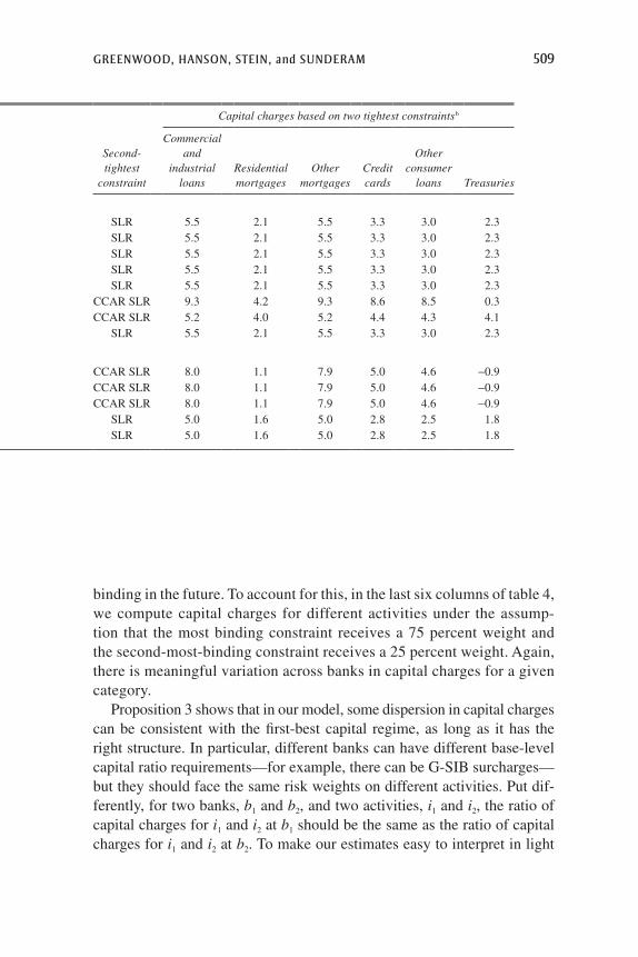
GREENWOOD, HANSON, STEIN, and SUNDERAM 509
binding in the future. To account for this, in the last six columns of table 4, we compute capital charges for different activities under the assump-tion that the most binding constraint receives a 75 percent weight and the second-most-binding constraint receives a 25 percent weight. Again, there is meaningful variation across banks in capital charges for a given category.
Proposition 3 shows that in our model, some dispersion in capital charges can be consistent with the first-best capital regime, as long as it has the right structure. In particular, different banks can have different base-level capital ratio requirements—for example, there can be G-SIB surcharges—but they should face the same risk weights on different activities. Put dif-ferently, for two banks, b1 and b2, and two activities, i1 and i2, the ratio of capital charges for i1 and i2 at b1 should be the same as the ratio of capital charges for i1 and i2 at b2. To make our estimates easy to interpret in light
Table 4. Estimated Capital Chargesa
Tightest constraint
Capital charges based only on tightest constraint
Second- tightest
constraint
Capital charges based on two tightest constraintsb
Bank
Commercial and
industrial loans
Residential mortgages
Other mortgages
Credit cards
Other consumer
loans Treasuries
Commercial and
industrial loans
Residential mortgages
Other mortgages
Credit cards
Other consumer
loans Treasuries
G-SIBsJPMorgan Chase CCAR SLR 5.7 1.1 5.7 2.8 2.4 1.3 SLR 5.5 2.1 5.5 3.3 3.0 2.3Bank of America CCAR SLR 5.7 1.1 5.7 2.8 2.4 1.3 SLR 5.5 2.1 5.5 3.3 3.0 2.3Citigroup CCAR SLR 5.7 1.1 5.7 2.8 2.4 1.3 SLR 5.5 2.1 5.5 3.3 3.0 2.3Morgan Stanley CCAR SLR 5.7 1.1 5.7 2.8 2.4 1.3 SLR 5.5 2.1 5.5 3.3 3.0 2.3Goldman Sachs CCAR SLR 5.7 1.1 5.7 2.8 2.4 1.3 SLR 5.5 2.1 5.5 3.3 3.0 2.3Wells Fargo Tier 1 10.5 5.3 10.5 10.5 10.5 0.0 CCAR SLR 9.3 4.2 9.3 8.6 8.5 0.3BNY Mellon SLR 5.0 5.0 5.0 5.0 5.0 5.0 CCAR SLR 5.2 4.0 5.2 4.4 4.3 4.1State Street CCAR SLR 5.7 1.1 5.7 2.8 2.4 1.3 SLR 5.5 2.1 5.5 3.3 3.0 2.3
Other large bank holding companiesU.S. Bancorp CCAR Tier 1 8.7 1.1 8.7 5.8 5.4 -1.7 CCAR SLR 8.0 1.1 7.9 5.0 4.6 -0.9PNC Financial CCAR Tier 1 8.7 1.1 8.7 5.8 5.4 -1.7 CCAR SLR 8.0 1.1 7.9 5.0 4.6 -0.9Capital One CCAR Tier 1 8.7 1.1 8.7 5.8 5.4 -1.7 CCAR SLR 8.0 1.1 7.9 5.0 4.6 -0.9HSBC CCAR SLR 5.7 1.1 5.7 2.8 2.4 1.3 SLR 5.0 1.6 5.0 2.8 2.5 1.8TD Bank CCAR SLR 5.7 1.1 5.7 2.8 2.4 1.3 SLR 5.0 1.6 5.0 2.8 2.5 1.8
Source: Authors’ calculations.a. This table reports capital charges Kbi = kb × ωi for different banks b and different loan categories i, where kb is
the minimum capital ratio for the most binding capital constraint facing bank b and ωi is the risk weight on activity i.b. We give 75 percent weight to the most binding capital constraint, and 25 percent weight to the second most
binding capital constraint. To determine the most binding constraint, we assume that the G-SIB surcharges are fully phased in to their January 2019 levels.

510 Brookings Papers on Economic Activity, Fall 2017
Figure 1. Estimated Capital Charges associated with Different Activitiesa
JPM
orga
n C
hase
Ban
k of
Am
eric
a
Citi
grou
p
Mor
gan
Sta
nley
Gol
dman
Sac
hs
Wel
ls F
argo
BN
Y M
ello
n
Stat
e St
reet
U.S
. Ban
corp
PNC
Fin
anci
al
Cap
ital
One
HSB
C
TD
Ban
k
Commercial and industrial loans
JPM
orga
n C
hase
Ban
k of
Am
eric
a
Citi
grou
p
Mor
gan
Sta
nley
Gol
dman
Sac
hs
Wel
ls F
argo
BN
Y M
ello
n
Stat
e St
reet
U.S
. Ban
corp
PNC
Fin
anci
al
Cap
ital
One
HSB
C
TD
Ban
k
Residential mortgagesJP
Mor
gan
Cha
se
Ban
k of
Am
eric
a
Citi
grou
p
Mor
gan
Sta
nley
Gol
dman
Sac
hs
Wel
ls F
argo
BN
Y M
ello
n
Stat
e St
reet
U.S
. Ban
corp
PNC
Fin
anci
al
Cap
ital
One
HSB
C
TD
Ban
k
Other mortgagesJP
Mor
gan
Cha
se
Ban
k of
Am
eric
a
Citi
grou
p
Mor
gan
Sta
nley
Gol
dman
Sac
hs
Wel
ls F
argo
BN
Y M
ello
n
Stat
e St
reet
U.S
. Ban
corp
PNC
Fin
anci
al
Cap
ital
One
HSB
C
TD
Ban
k
Credit cards
2
6
10
2
6
10
2
6
10
JPM
orga
n C
hase
Ban
k of
Am
eric
a
Citi
grou
p
Mor
gan
Sta
nley
Gol
dman
Sac
hs
Wel
ls F
argo
BN
Y M
ello
n
Stat
e St
reet
U.S
. Ban
corp
PNC
Fin
anci
al
Cap
ital
One
HSB
C
TD
Ban
k
Other consumer loans
1
3
5
2
6
10
0
2
4
JPM
orga
n C
hase
Ban
k of
Am
eric
a
Citi
grou
p
Mor
gan
Sta
nley
Gol
dman
Sac
hs
Wel
ls F
argo
BN
Y M
ello
n
Stat
e St
reet
U.S
. Ban
corp
PNC
Fin
anci
al
Cap
ital
One
HSB
C
TD
Ba n
k
Percent Percent
Percent Percent
Percent Percent
Treasuries
Source: Authors’ calculations. a. The sample includes bank holding companies based in the United States with total assets over $250 billion
in December 2016 and all bank holding companies classified as G-SIBs at that time. The figure plots, for each activity and each bank, the capital charge implied by the bank’s most binding constraint out of the four we consider: (i) the Tier 1 capital ratio in December 2016, (ii) the supplementary leverage ratio in December 2016, (iii) the minimum poststress Tier 1 capital ratio in the 2017 CCAR, and (iv) the minimum poststress supplemen-tary leverage ratio in the 2017 CCAR. To determine the most binding constraint, we assume that the G-SIB surcharges are fully phased in to their January 2019 levels.

GREENWOOD, HANSON, STEIN, and SUNDERAM 511
of this observation, in table 5 we normalize capital charges within each bank. Specifically, for each bank, we divide its estimated capital charge for each activity by its estimated capital charge for C&I loans, so that the resulting numbers can be thought of as a set of relative risk weights. Again, this is where proposition 3 gives us the clearest guidance; it says that differences across banks in these relative weights are precisely what creates the potential for distortions in resource allocation. As can be seen in table 5, there is indeed substantial variation across banks in these nor-malized capital charges. For example, residential mortgages have a rela-tive risk weight (as compared with C&I loans) of 100 percent for BNY Mellon and 50 percent for Wells Fargo, but only 19 percent for a number of other banks, including Bank of America and Citigroup. Such varia-tion is also apparent in the second panel of table 5, where we allow each bank to be subject to multiple binding constraints. This would seem to suggest a significant incentive for activity to migrate in an inefficient way across banks.
To get a back-of-the-envelope sense for the magnitudes involved, assume that—in violation of the Modigliani–Miller conditions—there is a non-risk-based “money” premium on deposits and short-term bank debt due to their usefulness as a transactions medium. An upper-bound estimate of this money premium might be on the order of 2 percentage points. Now con-sider banks’ decisions to engage in credit card lending. As shown in table 4, Wells Fargo faces a capital charge of 10.5 percent for credit cards, while the corresponding figure for Goldman Sachs is only 2.8 percent. Thus, this 7.7 percentage point differential would raise Wells Fargo’s overall cost of capital for credit card loans by 0.15 percent (= 7.7 percent × 2 percent) relative to that for Goldman Sachs.
Viewed as a potential change in the ultimate cost of credit to consumers, a 15 basis point regulatory wedge may not sound economically meaning-ful. However, as argued by Hanson, Kashyap, and Stein (2011), even rela-tively small differences in funding costs can have powerful effects on where the activity in question gets done. Unlike many other industries, banks’ most important competitive edge is their ability to fund themselves cheaply. Thus, if Wells Fargo is forced to adopt a capital structure that raises its cost of funding for credit cards relative to Goldman Sachs by 0.15 percent, it may eventually lose a meaningful chunk of its credit card business (or become less profitable, because the return on assets in bank-ing is on the order of 1 percent). Contrast this with, say, the automobile industry, where cheap financing is only one of many possible sources of advantage; a strong brand, high-quality engineering and customer service,
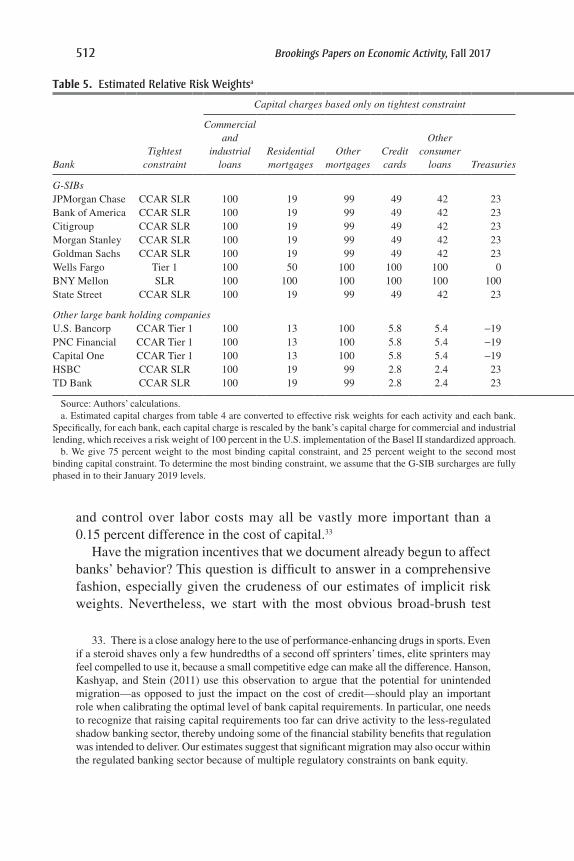
512 Brookings Papers on Economic Activity, Fall 2017
Table 5. Estimated Relative Risk Weightsa
BankTightest
constraint
Capital charges based only on tightest constraint
Second- tightest
constraint
Capital charges based on two tightest constraintsb
Commercial and
industrial loans
Residential mortgages
Other mortgages
Credit cards
Other consumer
loans Treasuries
Commercial and
industrial loans
Residential mortgages
Other mortgages
Credit cards
Other consumer
loans Treasuries
G-SIBsJPMorgan Chase CCAR SLR 100 19 99 49 42 23 SLR 100 38 99 61 55 41Bank of America CCAR SLR 100 19 99 49 42 23 SLR 100 38 99 61 55 41Citigroup CCAR SLR 100 19 99 49 42 23 SLR 100 38 99 61 55 41Morgan Stanley CCAR SLR 100 19 99 49 42 23 SLR 100 38 99 61 55 41Goldman Sachs CCAR SLR 100 19 99 49 42 23 SLR 100 38 99 61 55 41Wells Fargo Tier 1 100 50 100 100 100 0 CCAR SLR 100 45 100 92 91 4BNY Mellon SLR 100 100 100 100 100 100 CCAR SLR 100 78 100 86 84 79State Street CCAR SLR 100 19 99 49 42 23 SLR 100 38 99 61 55 41
Other large bank holding companiesU.S. Bancorp CCAR Tier 1 100 13 100 5.8 5.4 -19 CCAR SLR 100 14 99 63 58 -11PNC Financial CCAR Tier 1 100 13 100 5.8 5.4 -19 CCAR SLR 100 14 99 63 58 -11Capital One CCAR Tier 1 100 13 100 5.8 5.4 -19 CCAR SLR 100 14 99 63 58 -11HSBC CCAR SLR 100 19 99 2.8 2.4 23 SLR 100 31 99 57 50 35TD Bank CCAR SLR 100 19 99 2.8 2.4 23 SLR 100 31 99 57 50 35
Source: Authors’ calculations.a. Estimated capital charges from table 4 are converted to effective risk weights for each activity and each bank.
Specifically, for each bank, each capital charge is rescaled by the bank’s capital charge for commercial and industrial lending, which receives a risk weight of 100 percent in the U.S. implementation of the Basel II standardized approach.
b. We give 75 percent weight to the most binding capital constraint, and 25 percent weight to the second most binding capital constraint. To determine the most binding constraint, we assume that the G-SIB surcharges are fully phased in to their January 2019 levels.
and control over labor costs may all be vastly more important than a 0.15 percent difference in the cost of capital.33
Have the migration incentives that we document already begun to affect banks’ behavior? This question is difficult to answer in a comprehensive fashion, especially given the crudeness of our estimates of implicit risk weights. Nevertheless, we start with the most obvious broad-brush test
33. There is a close analogy here to the use of performance-enhancing drugs in sports. Even if a steroid shaves only a few hundredths of a second off sprinters’ times, elite sprinters may feel compelled to use it, because a small competitive edge can make all the difference. Hanson, Kashyap, and Stein (2011) use this observation to argue that the potential for unintended migration—as opposed to just the impact on the cost of credit—should play an important role when calibrating the optimal level of bank capital requirements. In particular, one needs to recognize that raising capital requirements too far can drive activity to the less-regulated shadow banking sector, thereby undoing some of the financial stability benefits that regulation was intended to deliver. Our estimates suggest that significant migration may also occur within the regulated banking sector because of multiple regulatory constraints on bank equity.

GREENWOOD, HANSON, STEIN, and SUNDERAM 513
Table 5. Estimated Relative Risk Weightsa
BankTightest
constraint
Capital charges based only on tightest constraint
Second- tightest
constraint
Capital charges based on two tightest constraintsb
Commercial and
industrial loans
Residential mortgages
Other mortgages
Credit cards
Other consumer
loans Treasuries
Commercial and
industrial loans
Residential mortgages
Other mortgages
Credit cards
Other consumer
loans Treasuries
G-SIBsJPMorgan Chase CCAR SLR 100 19 99 49 42 23 SLR 100 38 99 61 55 41Bank of America CCAR SLR 100 19 99 49 42 23 SLR 100 38 99 61 55 41Citigroup CCAR SLR 100 19 99 49 42 23 SLR 100 38 99 61 55 41Morgan Stanley CCAR SLR 100 19 99 49 42 23 SLR 100 38 99 61 55 41Goldman Sachs CCAR SLR 100 19 99 49 42 23 SLR 100 38 99 61 55 41Wells Fargo Tier 1 100 50 100 100 100 0 CCAR SLR 100 45 100 92 91 4BNY Mellon SLR 100 100 100 100 100 100 CCAR SLR 100 78 100 86 84 79State Street CCAR SLR 100 19 99 49 42 23 SLR 100 38 99 61 55 41
Other large bank holding companiesU.S. Bancorp CCAR Tier 1 100 13 100 5.8 5.4 -19 CCAR SLR 100 14 99 63 58 -11PNC Financial CCAR Tier 1 100 13 100 5.8 5.4 -19 CCAR SLR 100 14 99 63 58 -11Capital One CCAR Tier 1 100 13 100 5.8 5.4 -19 CCAR SLR 100 14 99 63 58 -11HSBC CCAR SLR 100 19 99 2.8 2.4 23 SLR 100 31 99 57 50 35TD Bank CCAR SLR 100 19 99 2.8 2.4 23 SLR 100 31 99 57 50 35
Source: Authors’ calculations.a. Estimated capital charges from table 4 are converted to effective risk weights for each activity and each bank.
Specifically, for each bank, each capital charge is rescaled by the bank’s capital charge for commercial and industrial lending, which receives a risk weight of 100 percent in the U.S. implementation of the Basel II standardized approach.
b. We give 75 percent weight to the most binding capital constraint, and 25 percent weight to the second most binding capital constraint. To determine the most binding constraint, we assume that the G-SIB surcharges are fully phased in to their January 2019 levels.
in figure 2. Here we look at how the ratio of risk-weighted assets to total assets changes between 2012:Q4 and 2016:Q4 as a function of the initial ratio in 2012:Q4. The idea is that risk-based capital rules are more likely to bind for banks with high initial ratios of risk-weighted assets to total assets. Thus, for these banks, activities with low risk weights should be attractive at the margin. As they shift toward such activities, their ratios of risk-weighted assets to total assets should fall. In contrast, for banks with low initial ratios of risk-weighted assets to total assets, the SLR is more likely to bind, making those activities that have high risk weights more attractive. Thus, for these banks, the ratio of risk-weighted assets to total assets should rise.34 This is exactly what we see in figure 2: In a regression
34. Flannery, Hirtle, and Kovner (2017) conduct a related exercise. They regress loan growth in a given category on the difference between the Federal Reserve’s estimated loan losses for a bank under the severely adverse scenario and the bank’s own estimated losses. They find little evidence of a relationship.
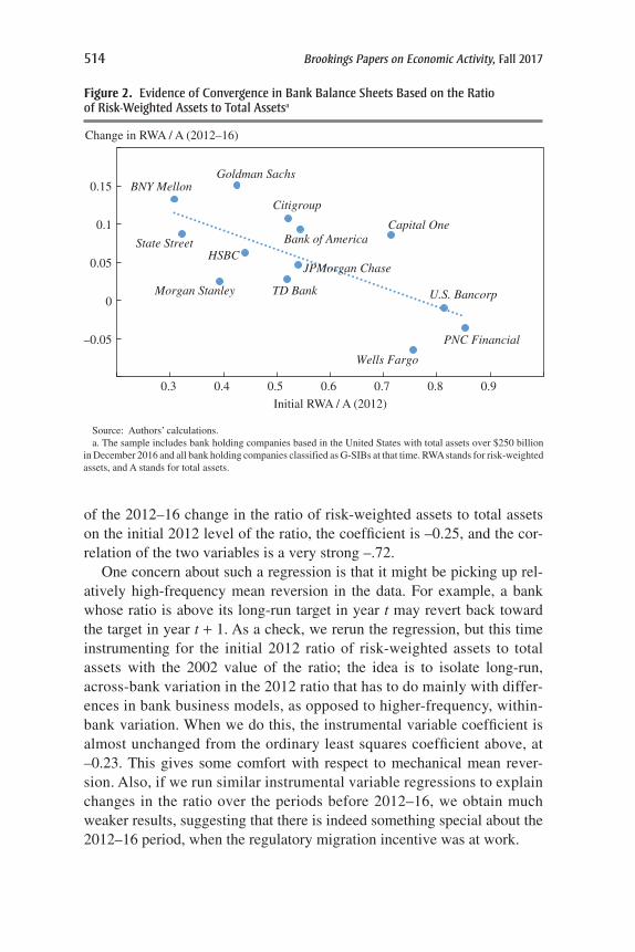
514 Brookings Papers on Economic Activity, Fall 2017
of the 2012–16 change in the ratio of risk-weighted assets to total assets on the initial 2012 level of the ratio, the coefficient is –0.25, and the cor-relation of the two variables is a very strong –.72.
One concern about such a regression is that it might be picking up rel-atively high-frequency mean reversion in the data. For example, a bank whose ratio is above its long-run target in year t may revert back toward the target in year t + 1. As a check, we rerun the regression, but this time instrumenting for the initial 2012 ratio of risk-weighted assets to total assets with the 2002 value of the ratio; the idea is to isolate long-run, across-bank variation in the 2012 ratio that has to do mainly with differ-ences in bank business models, as opposed to higher-frequency, within-bank variation. When we do this, the instrumental variable coefficient is almost unchanged from the ordinary least squares coefficient above, at –0.23. This gives some comfort with respect to mechanical mean rever-sion. Also, if we run similar instrumental variable regressions to explain changes in the ratio over the periods before 2012–16, we obtain much weaker results, suggesting that there is indeed something special about the 2012–16 period, when the regulatory migration incentive was at work.
Figure 2. Evidence of Convergence in Bank Balance Sheets Based on the Ratio of Risk-Weighted Assets to Total Assetsa
Source: Authors’ calculations.a. The sample includes bank holding companies based in the United States with total assets over $250 billion
in December 2016 and all bank holding companies classified as G-SIBs at that time. RWA stands for risk-weighted assets, and A stands for total assets.
JPMorgan Chase
Bank of America
Citigroup
Morgan Stanley
Goldman Sachs
Wells Fargo
BNY Mellon
State Street
U.S. Bancorp
PNC Financial
Capital One
HSBC
TD Bank
–0.05
0
0.05
0.1
0.15
0.3 0.4 0.5 0.6 0.7 0.8 0.9
Initial RWA / A (2012)
Change in RWA / A (2012–16)

GREENWOOD, HANSON, STEIN, and SUNDERAM 515
Finally, the patterns in figure 2 are consistent with the idea that the rela-tive tightness of the various constraints for different banks reflects hetero-geneity in their underlying business models. The banks that have reduced risk-weighted assets the most are U.S. Bancorp, PNC Financial, and Wells Fargo, all of which are traditional commercial banks that naturally tend to be most bound by either the Tier 1 ratio or the poststress Tier 1 ratio. The banks that have reduced risk-weighted assets the least are the two cus-tody banks, BNY Mellon and State Street, as well as Goldman Sachs, whose businesses all require large holdings of relatively low-risk secu-rities, and which therefore are more likely to be bound by the SLR or poststress SLR.35
Suppose we take figure 2 at face value—that is, we take it as evidence of the sort of inefficient migration described in proposition 3. An important question—to which we do not have a satisfactory answer at this point—is then: Just how big are the welfare costs associated with this regulation-induced migration? In the literal context of the model, the welfare loss is simply that too much of certain types of lending ends up being done by banks with high operating costs. Stepping outside the model, one can imag-ine two potentially more worrisome consequences. First, banks might be encouraged to enter new lines of business where they have little expertise or experience, and where their risk management capabilities are not well developed. This could lead to an accumulation of poorly understood risks in the wrong hands. And second, to the extent that the result of migration is an industry configuration where the major players are driven toward hav-ing similar business models, this would raise the probability that many of them could become undercapitalized at the same time, which might set off the kinds of amplification mechanisms seen in the global financial crisis. Again, however, we do not have a good understanding of just how quanti-tatively important either of these effects might be.
II.C. What About Uncertainty and Regulatory Arbitrage?
The logic of the model speaks clearly to the desirability of having a single risk-based capital rule, and to the distortions associated with having multiple potentially binding rules. But perhaps rules that do not emerge naturally in our framework, like the SLR, can be rationalized by appeal-ing to factors that have been left out of our simple model. We discuss
35. One concrete example of the pattern documented in figure 2 is Goldman Sachs’s recent push into traditional bank lending activities (Hoffman 2017). Another is Wells Fargo’s move into the capital markets and investment banking businesses (Freed 2016).

516 Brookings Papers on Economic Activity, Fall 2017
three potential rationales for imposing multiple rules that are outside our model: dealing with Knightian uncertainty (Knight 1921), responding to regulatory arbitrage, and providing banks with appropriate incentives to diversify.
A first potential rationale for simultaneously imposing both a risk-based capital requirement and a non-risk-based leverage requirement is that doing so adds robustness when there is Knightian uncertainty about the riskiness of different asset categories—in contrast to our assumption that the regula-tor knows the true risk model that governs the probability of bank failure. However, on closer inspection, this argument has a couple of weak spots. The most direct implication of uncertainty about the true model is that the regulator should use a single system of risk weights, which reflects an appropriate average of the weights implied by different candidate models. Note that this “averaging” approach is not the same thing as having mul-tiple independent constraints if banks have heterogeneous business models, as in proposition 3. In the latter case, different banks will place different weights on the two constraints, which creates the migration problems dis-cussed above but does not help further the robustness objective.
Moreover, having one of the constraints be a wholly risk-insensitive leverage requirement is tantamount to putting some weight on a model of the world in which all assets have the same risk. Although it seems sensible enough to argue in favor of increasing the risk weights some-what on the lowest-risk assets—on the theory that these assets might be riskier than is commonly supposed—it is hard to see why this same logic cuts in favor of sharply reducing the risk weights on very high-risk assets. In summary, a Knightian form of model uncertainty suggests the use of a single risk-based capital requirement that averages across plau-sible risk models; it does not cut in favor of a regime with two redundant requirements, particularly not one that includes a risk-insensitive lever-age requirement.
Alternatively, a defender of the SLR might argue that the conclusions from the model rest on a particularly unrealistic feature: The model assumes that banks’ risk choices are observable and contractible, that is, the regula-tor observes the risk associated with loans in category i, and thus can assign the proper risk weight ex ante. This amounts to assuming away the pos-sibility of regulatory arbitrage. However, in reality, vulnerability to such arbitrage is an absolutely central problem for regulation. That is, there is always the danger that a bank finds a way to make a high-risk loan yet have it be categorized as relatively low-risk for the purposes of measuring risk-weighted assets.
GREENWOOD, HANSON, STEIN, and SUNDERAM 517
Moreover, it is exactly these sorts of concerns about regulatory arbitrage that have motivated advocates of the SLR. Some of these observers note that an unweighted leverage ratio can be a useful backstop to the risk-based regime, because if a bank has a high ratio of unweighted assets to risk-weighted assets, this is a clue that it may be gaming the risk-based regime, so one might want to impose another constraint that limits this gaming. Others, like Thomas Hoenig (2016), vice chairman of the Federal Deposit Insurance Corporation (FDIC), go further, arguing that a leverage ratio should be the primary tool of bank capital regulation: “Risk-based capi-tal schemes encouraged banks to use their financial engineering tools to increase leverage and reported returns associated with artificially low risk-weighted asset classes. Low weights were assigned to subprime mortgages, foreign sovereign debt, collateralized debt obligations, and derivatives, like credit default swaps. These asset classes ended up dominating the banks’ balance sheets, leading to massive losses.”36
Again, we take these gaming concerns extremely seriously, and think that they need to be addressed head-on in any system of capital regulation. However, if one wants to attack regulatory arbitrage most effectively, it may be necessary to change the timing of the interaction between the regu-lator and the banks. The problem with an entirely rules-based system is that the regulator moves first, setting the rules in stone, after which the bank gets to move second, optimizing against the now rigid and therefore easily exploitable set of rules. Ideally, to curb arbitrage, it would help to let the regulator have another go at the problem, after having observed the specific actions that the bank has taken in light of the ex ante rules, which were not contractible in advance.
Consider a concrete example. Suppose that the only ex ante rule in place is a poststress Tier 1 capital ratio requirement, of the sort described in equa-tion 3. Both the capital requirement kRBC,STRESS and the risk weights wi associ-ated with this rule have been fixed, and do not change from year to year. But consistent with the worries that have motivated the SLR, the regulator observes that ex post, once the rule is in place, banks are loading up to an unexpected degree on a particular type of loan i that has a low risk weight in the rule. Moreover, the regulator suspects that this is in part because i is exposed to a type of risk that was not adequately captured in the ex ante risk-weighting scheme, that is, to a risk that was not contractible ex ante but that has now been revealed to be important by the banks’ actions.
36. In a similar vein, Goldstein (2017, p. 9) writes: “The leverage ratio should thus be the primary capital standard, and risk-based measures should serve as a backup.”

518 Brookings Papers on Economic Activity, Fall 2017
We would argue that a better response is not to impose another rigid ex ante rule as a patch on the first but rather to use the stress-testing process to fill in this ex post observable contingency after the fact. For example, the stress test in year t could be designed to make particularly pessimistic assumptions about loan losses on any loan type i that has grown unex-pectedly rapidly in the past year or two. That is, though the kRBC,STRESS and wi parameters in equation 3 would be fixed in advance and time-invariant, the NLRi term, which depends on the loss assumptions embedded in the stress test, would be allowed to vary year by year. Moreover, if done in the way that we have in mind, much of the year-to-year variation in stress test scenarios would be driven not just by changes in the macroeconomic environment but also by supervisors’ observations of granular changes in the composition of bank portfolios.
Finally, recall that optimal risk-based capital requirements only take the linear, portfolio-invariant form used in practice if losses on different bank asset categories are perfectly correlated. Thus, a last argument in favor of imposing a leverage requirement alongside a risk-based requirement might be that this is an indirect way of implementing the nonlinear, portfolio-dependent capital requirement that is optimal in setting where different asset categories are imperfectly correlated. For example, suppose losses on credit card loans are imperfectly correlated with losses on C&I loans. This means that the optimal marginal capital charge on credit card loans should be higher at banks whose portfolios are tilted toward credit cards than at banks whose portfolios are tilted toward C&I loans. In this way, a well-designed system of portfolio-dependent capital rules would provide banks with the appropriate incentives to diversify their portfolios across different asset categories.
However, it seems difficult to argue that the current set of capital require-ments comes close to approximating this optimal portfolio-dependent rule. Specifically, the combination of the SLR and risk-based requirements only encourages diversification across risk weight buckets, but not within risk weight buckets (for example, within assets that all carry a 100 percent risk weight). Thus, in practice, we suspect that this combination of constraints does very little to encourage diversification within the traditional banking book, where most assets have high risk weights, or within the trading book, where many assets have low risk weights. Instead, we suspect that it pri-marily has the effect of encouraging diversification across the banking and trading books—that is, of encouraging all large banks to become universal banks engaged in both commercial banking and trading. This is clearly not the intended purpose of the regulatory regime.

GREENWOOD, HANSON, STEIN, and SUNDERAM 519
III. Dynamic Considerations
The version of the model developed in section II was meant to speak to a steady-state situation, where the dollar value of equity in the bank-ing system had somehow gravitated to its long-run, first-best level, so that we could ignore the flow adjustment costs associated with rais-ing external equity finance. We now consider what the logic of this framework says about how regulation should be designed away from the steady state, when a negative shock has reduced bank equity sig-nificantly below the first-best level, and where flow costs therefore take center stage.
To be concrete, assume that a shock has lowered bank equity at time 0 to E0, which is lower than the first-best value of E* implicit in proposition 1. Assume further that by time 2, banks will have worked their way out of this hole—say, by retaining sufficient earnings—and we will be back at the first-best steady state. As a result, the social planner’s only dynamic prob-lem lies in deciding what should happen at time 1—that is, deciding on the transition path back to the steady state.
Thus, at time 1, the planner is faced with the following welfare function:
W f A c E E E X ki ii
N
∑ ( ) ( )( ) ( )= − − λ − − π=
(9) ,1 1 1 1 0 11
where k1 ≡ E1/(∑Ni=1wi Ai1). This looks similar to the welfare function in the
steady-state case, with the addition of one new term, λ(E1 – E0), where λ(⋅) is an increasing, convex function that captures the flow cost of adjusting equity upward from E0 to E1 between time 0 and time 1. In other words, the planner now faces a new tension: If the goal is to get lending moving back up toward its first-best level, without tolerating an increased probability of bank failure at time 1, this will necessarily involve bearing some flow costs of external finance.
Similarly, the bank’s objective function is now to maximize
B f A c E E E X ki ii
N
∑ ( ) ( ) ( )( )( ) ( )= − − + θ λ − − − φ π=
(10) 1 1 .1 1 1 1 0 11
Note that there are now two sources of divergence between the bank and the planner. First, as before, the bank underinternalizes the social costs
520 Brookings Papers on Economic Activity, Fall 2017
of bank failure; this is captured in the (1 – φ) term in its objective func-tion. And second, the bank now also views the flow costs of raising new external finance to be more burdensome than the planner does; this is reflected in the assumption that θ > 0. This latter wedge can be thought of as rooted in external financing frictions due to debt overhang (Myers 1977) or asymmetric information (Myers and Majluf 1984). These fric-tions make new equity issues costly from the perspective of bank share-holders; but because they are either transfers between shareholders and creditors (in the case of debt overhang) or transfers between old and new shareholders (in the case of asymmetric information), they do not represent a social cost.
With these assumptions in place, and under the natural regularity condi-tions given in the online appendix, we establish the following proposition.
Proposition 4. Optimal regulation in the wake of an adverse shock can be char-acterized as follows: (i) The cross-sectional risk weights, wi, are unchanged from the steady-state case; (ii) there is temporary “capital ratio relief,” in that the required capital ratio, k1*, is set at a lower value than the steady-state opti-mum of k*, implying a higher probability of failure, π(k1*); and (iii) banks must be forced to raise new external equity, meaning that the regulator requires the banks to have equity of E1*, which is higher (and therefore closer to the long-run, first-best value of E*) than would be chosen by the bank if it were only facing the ratio-based capital requirement k1*.
Thus, the appropriate response to an adverse shock is twofold; banks should be temporarily allowed to operate at lower capital ratios than in normal times, but at the same time they should be compelled to raise new dollars of external equity finance. The intuition for the first piece is most easily seen by considering the polar case, where the social flow costs of external finance are infinite. In this case, bank equity is fixed at a level lower than the first-best one, and the planner faces the following trade-off: Keep the same capital ratio requirement as before, in which case bank lending will be cut below the first-best outcome, or reduce the capital ratio requirement and accept a higher probability of bank failure. In an interior solution, optimality will involve some adjustment on both margins; hence, the motive for capital ratio relief.
The logic for compelling new equity raises comes through most clearly when the social flow costs of raising external equity are small but the pri-vate flow costs of raising equity are large, that is, when λ(⋅) ≈ 0 and θ >> 0. Here, a bank left to its own devices would be inclined to cut lending sharply in order to comply with a given capital ratio requirement, because this allows it to avoid having to raise new equity. However, the planner,

GREENWOOD, HANSON, STEIN, and SUNDERAM 521
who does not care nearly as much about the flow costs of equity issuance, would prefer to see the bank maintain its lending.37
Of these two methods of responding to an adverse shock—capital ratio relief, and forced equity issues—we see the latter as the more pragmati-cally relevant, for two reasons. First, though the corporate finance literature has amply documented the importance of flow costs of external finance, the best-understood mechanisms are those that involve private costs, and not social costs, with debt overhang and asymmetric information being the leading examples (Myers 1977; Myers and Majluf 1984; Greenwald, Stiglitz, and Weiss 1984). In this case, where λ(⋅) ≈ 0 and θ >> 0, the right response is to give relatively less in the way of capital ratio relief, and to focus primarily on getting new dollars of equity into the banking system.
Second, even if the regulator is willing to extend temporary relief in the capital ratio, it may be hard to get banks to accept this relief in practice. A bank whose required capital ratio is cut temporarily knows that the require-ment will eventually revert back to a higher steady-state value. It may thus be reluctant to operate much below the long-run value, preferring instead to cut lending so as to more rapidly get back into long-run compliance, particularly if there are perceived reputational costs for operating below the long-run target value. Nevertheless, to the extent that some degree of capital ratio relief can be implemented, it is likely to be a useful part of the overall tool kit when the banking system is under stress, and this should be borne in mind when designing the regulatory regime. Indeed, the so-called capital conservation buffer in the risk-based rule can be thought of as being somewhat in this spirit. Also, we discuss a related alternative below.
IV. Policy Recommendations
The preceding discussion yields three core principles that should inform the design of capital regulation.
CONSOLIDATE CONSTRAINTS As we have argued, having multiple inde-pendent constraints on bank equity ratios is problematic. When different constraints bind for different banks—as is clearly the case in the data—this is equivalent to imposing different marginal tax rates on the same activity across different institutions. The result is long-run pressure for the industry to adjust in such a way as to create unintended convergence in banks’ busi-ness models, even when this convergence does not reflect their inherent
37. Again, this is the essence of the macroprudential argument made informally by Hanson, Kashyap, and Stein (2011), among others. See also Sarin and Summers (2016).

522 Brookings Papers on Economic Activity, Fall 2017
competitive strengths. We are already seeing some evidence of this phe-nomenon in the sharply reduced dispersion of the ratio of risk-weighted assets to total assets across the largest banks, as shown in figure 2. And absent a change in regulatory approach, we are likely to see other worri-some symptoms of noneconomic industry-level adaptation. The straight-forward solution is to dispense with the multiple constraints and to replace them with a single constraint that is as well designed as possible. We pro-vide some detail on how this might be done in the next subsection.
ADDRESS REGULATORY ARBITRAGE BY FILLING IN CONTINGENCIES EX POST No set of ex ante rules, no matter how granular or sophisticated, can satis-factorily tackle the problem of regulatory arbitrage; once any set of rules has been put in place, the second-mover advantage of the banks is just too great. Instead, regulators need to retain flexibility to adjust some com-ponents of capital requirements ex post. One way to do this is by having each year’s CCAR stress scenarios be responsive to incoming clues about gaming coming from rapid growth or surprisingly high profitability in par-ticular lines of activity.
DYNAMIC RESILIENCE Our model suggests that in the wake of a large negative shock to the banking system, the optimal response involves both (i) allow-ing required capital ratios to decline temporarily and (ii) compelling banks to cut their payouts and issue new external equity. The latter of these is particularly important, and indeed was one of the central design fea-tures of the 2009 SCAP. It is therefore crucial that the CCAR process and infrastructure be designed in such a way as not to devolve solely into an appendage to capital ratio regulation in normal times, but rather also stand ready to implement an SCAP-like recapitalization of the industry when the time comes.
These three principles in turn lead us to specific recommendations for updating and strengthening the current capital regulation regime, which are outlined in the following subsections.
IV.A. Dial Back the Supplementary Leverage Ratio
As we have argued at length, having an SLR that is either binding or near-binding is counterproductive and distortionary. There are two broad ways that the SLR could be made to be less constraining on bank behav-ior. First, the minimum level of the ratio could be reduced, for example, from 5 to 3 percent for the G-SIBs. Alternatively, as recommended in the Treasury Department’s June 2017 report (Mnuchin and Phillips 2017), the denominator of the ratio could be adjusted to exclude the very safest assets, including (in the Treasury’s formulation) central bank reserves,

GREENWOOD, HANSON, STEIN, and SUNDERAM 523
38. A third way would be to sharply increase risk-based requirements, which would also have the effect of making the SLR less binding.
39. We also suspect that rapid balance sheet growth in a given asset category is likely to be a more general and more reliable early indicator of credit market overheating than this backstop rule binding more tightly. This is because this backstop rule would only bind more tightly when credit growth was concentrated in assets with low risk weights.
Treasury securities, and the initial margin for centrally cleared deriva-tives.38 In principle, either approach could serve the desired purpose, so we do not have a strong view as to which is preferable. But if forced to choose, we might pick the former, because the latter could create a sharp cliff between Treasuries, which would now have a risk weight of zero, and near-riskless substitutes (for example, agency and highly rated corporate bonds). However, to the extent that either approach makes the SLR much less likely to bind at all, this distinction may not matter much in practice.
Although we urge a reduced role for the SLR, we share many of the concerns that have motivated its advocates, such as (i) the general potential for the current risk-based regime to be gamed; (ii) the particular vulner-ability to such gaming of complex, model-based approaches to setting risk weights; and (iii) the lack of any risk weight at all on sovereign securities, even those that are relatively risky. We therefore attempt to address these concerns in our remaining recommendations.
To be clear, if we take the logic of our model literally, it implies that the SLR should be eliminated entirely, whereas as a pragmatic policy recom-mendation, we are more comfortable only suggesting that it be dialed back significantly. In part, this is because the alternative—and more discretionary— antigaming approaches that we propose are as yet untested, and either may not be adopted or may not work as well as we would hope. If so, there may be some robustness merit in having an alternative, backstop, rules-based regime that is calibrated in such a way that it has little impact on behavior in normal times, and yet can serve as a flag that prompts regulatory action when there is a credit boom that is concentrated in assets with relatively low statutory risk weights. Even in this case, we doubt that the optimal backstop rule would look exactly like a wholly risk-insensitive leverage ratio; but it might have the general feature of pushing up the risk weights for those asset categories that are given low weights under the primary regime. Also, we believe that much of the value of having such a backstop rule is that it would prompt regulatory action ex post—that is, it too would necessarily rely on regulatory discretion.39

524 Brookings Papers on Economic Activity, Fall 2017
IV.B. Integrate the Risk-Based Capital Requirement and the CCAR into a Single Constraint
One way to accomplish this integration is put forward by Daniel Tarullo (2017) and Nellie Liang (2017b), drawing on ongoing staff work at the Federal Reserve. The idea is that there would just be a single, over arching, risk-based capital requirement. It would start with a baseline risk-based ratio, similar to that in our equation 1; but then this ratio would be aug-mented with a “stress capital buffer” that incorporates estimates of net losses coming from the annual CCAR process. Tarullo (2017) explains the concept as follows:
The proposal for what our staff has called a “stress capital buffer” would simplify our capital regime by replacing the existing 2.5 percent fixed capital conserva-tion buffer applicable to all banks with a buffer requirement equal to the maxi-mum decline in a firm’s common equity ratio under the severely adverse scenario of the stress test.
Also, this stress capital buffer would be subject to a 2.5 percent floor.Although there are various ways to work out the details, the conceptual
point to note is that this would replace equation 1 with a more explicit version of what we have already derived as the implicit poststress capi-tal requirement in equation 3. Specifically, Tarullo’s description corre-sponds to an aggregate dollar equity requirement of E = k × RWA + NET-STRESS-LOSSES, for some value of the baseline capital ratio k. And indeed, an aggregate dollar requirement like this is exactly what one gets by aggregating up the category-level capital charges in equation 3—which, recall, were of the general form (with subscripts now omitted) Ki ≈ k × wi + NLRi.40
In other words, each bank would now face just a single constraint, and the effective risk weight for any asset i would be the sum of a statutory, time-invariant, Basel-style risk weight wi and a component that reflects asset i’s performance in the severely adverse stress scenario. Moreover, the latter piece would not be set in stone but could vary year to year. Although there would be time variation in risk weights, the fact that there is only a single binding constraint at any point in time implies that all banks face the same cross-sectional tax rates on their activities, which is
40. The risk-based requirement would take the form E = (k + kSCB) × RWA, where k is the base-line risk-based ratio (6 percent for Tier 1 capital) and k E RWA E RWASTRESSSCB [ ]( )= −max 2.5, percent. Assuming kSCB > 2.5 percent and E – ESTRESS = ∑N
i=1 NLRi Ai + CONSTANT, this implies a capital charge of Ki = k × wi + NLRi for asset i.
GREENWOOD, HANSON, STEIN, and SUNDERAM 525
the key to minimizing the sorts of industry-level distortions that we have emphasized.41
IV.C. Design Annual Stress Scenarios with Regulatory Arbitrage in Mind
At first glance, one reaction to a consolidated constraint of the sort described just above might be that it is only a relabeling of the usual risk-based capital requirement. If so, one might ask what the indepen-dent role of the stress-testing process is—that is, why do we need the CCAR when it is simply being folded into the conventional, risk-based capital regime?
Again, the point to emphasize is that if capital charges are of the form Ki ≈ k × wi + NLRi, this differs from the traditional risk-based regime because the component contributed by the CCAR—namely, NLRi—is not a time-invariant constant based on a rulemaking process like the usual risk weights wi but rather is free to vary with each year’s design of the stress scenario. To take maximum advantage of this flexibility, it should be used proactively to combat regulatory arbitrage. As noted above, one way to do this would be to purposefully design each year’s CCAR stress scenarios to react to rapid growth or surprisingly high profitability in particular lines of activity. This could be done at quite a granular level. Indeed, a natural starting point for the exercise might be, for example, to have supervisors ask who the 20 most highly compensated line managers or traders are in each big bank each year, and then to think about stress testing the expo-sures most closely associated with these employees.42 The underlying idea is to learn as much as possible about the incentives at play by observing the
41. Tarullo (2016) and Liang (2017b) have proposed folding the G-SIB surcharge into the baseline ratio used in this blended approach, implying a capital charge of Kbi = kb × wi + NLRi for bank b’s holdings of loans in category i. Since NLRi is constant across banks, this capital charge does not take the desired form Kbi = kb × ωi for some set of effective risk weights, ωi. However, the logic underlying G-SIB surcharges suggests that regula-tors should ask G-SIBs to hold more capital against tail events—that is, against losses in a severely adverse scenario—than non G-SIBs. This then suggests capital charges of the form K k w NLR k kbi b i b ii
( )= × + = × ω , where k is the baseline ratio for a non-G-SIB. This cor-responds to a stress capital buffer of ( )[ ]= −×k k k E RWA E RWAb b b STRESS b bSCB b max 2.5, ,, percent, and a total capital requirement of Eb = (kb + kSCB,b) × RWAb for G-SIB b.
42. An approach of this sort may well have surfaced the “London Whale” risk expo-sures that lost JPMorgan Chase over $6 billion in 2012, as managers and traders respon-sible for the risk were among the highest paid in the organization (Levin and McCain 2013, pp. 57–59).

526 Brookings Papers on Economic Activity, Fall 2017
behavior of bank executives, and then to condition the CCAR design based on what is learned from this behavior.
IV.D. Basel-Style Risk Weights Should Be Simple and Not Based on Models
Although we do not agree with the leverage ratio approach of setting all risk weights equal to 1, we are highly sympathetic to the idea that risk weights should not be determined based on complicated models, much less banks’ own internal models. Doing so would seem to further invite various forms of gaming.
It should be noted that the complex methods based on internal models that increasingly came into vogue during the Basel II period were seemingly motivated by a desire on the part of regulators to get rules-based risk weights as close to “right” as possible, that is, similar to what would come out of a bank’s more economically driven internal portfolio optimization process. Although this was a noble goal, experience has taught us that it is difficult to implement such a precise level of risk sensitivity with a static set of prespec-ified rules because, once written down, they are so vulnerable to arbitrage.
We believe that a consolidated capital requirement that marries the risk-based and CCAR approaches is potentially promising on this dimension, in the following specific sense. Recall, again, that with this blended con-straint, capital charges take the general form Ki ≈ k × wi + NLRi, so the capital charge on asset i is only partly determined by the prespecified Basel risk weight wi, with the results from the CCAR process also left to do some of the job. Under this blended regime, it may be appropriate for the time-invariant wi to only attempt to capture relatively coarse distinctions in risk, and to let the values of NLRi, which come out of the CCAR—and hence are more flexible year to year and less vulnerable to gaming—be responsible for the more granular risk distinctions.
For example, it may well make sense to have different prespecified risk weights wi for broad categories of bank assets as under Basel II’s standard-ized approach; unsecured consumer loans might have different weights than C&I loans or mortgages, and all these would certainly have different risk weights than Treasuries. At the same time, it may be less productive to use a predetermined set of internal bank models to try to make finer ex ante distinctions between loans to consumers who have different demo-graphic or income profiles, or who are living in different parts of the coun-try. Perhaps it would be better in this case to see how the banks behave; and if they appear ex post to be tilting heavily to one subcategory of con-sumer loans, this should be incorporated in the next iteration of the CCAR.
GREENWOOD, HANSON, STEIN, and SUNDERAM 527
Thus, the overall philosophy would be to do somewhat less accounting for banks’ risk choices ex ante with complicated and highly granular formal risk weights, and more with a thoughtful ex post design of stress scenarios.
IV.E. Make Use of the Countercyclical Properties of the Stress Capital Buffer
Our model suggests another way to take advantage of the potential for time variation in the stress capital buffer. Recall that in the wake of a negative shock to banking system capital, one part of the optimal response is to relax the required capital ratio requirement in a countercyclical man-ner. This will happen naturally—and in a broadly symmetric way across banks—if there is a single capital requirement that incorporates a stress capital buffer, provided that the underlying stress scenario envisions less further deterioration in the macroeconomic environment once the economy has already declined significantly.43
This sort of macroeconomic sensitivity is already incorporated in the design of the underlying CCAR scenarios. But the current regime, with its multiple constraints, does not have as uniform a countercyclical effect on required capital, because not all banks are equally bound by the post-stress capital requirement. Moreover, though there is also a separate formal countercyclical buffer built into the standard risk-based Basel regime, thus far this buffer has not been deployed by U.S. regulators. This may in part reflect the political economy challenges associated with varying an explicit and highly visible statutory requirement. In contrast, if the countercyclical variation is instead an implicit by-product of changes in the annual CCAR assumptions, it may be easier to implement on a semidiscretionary basis.
IV.F. Consider Increasing G-SIB Surcharges
Although our model cautions about the potential distortions associated with imposing different cross-sectional risk weights on different banks, it also makes it clear that, holding the structure of these risk weights fixed, it can make good sense to set a higher overall minimum capital ratio for those banks whose failure would have higher social costs. In this sense, our model rationalizes the existence of something very much like G-SIB sur-charges. So these surcharges should continue to play a role in any blended
43. For example, when the unemployment rate is 5 percent, the severely adverse scenario might contemplate unemployment rising by 5 percentage points, to 10 percent. But when the unemployment rate has already hit 8 percent, the further increase modeled in the severely adverse scenario might only be 4 percentage points, to 12 percent. This would tend to reduce the going-forward stress capital buffer, all else equal.

528 Brookings Papers on Economic Activity, Fall 2017
requirement of the sort that we have discussed above—that is, the baseline capital ratio requirement should be higher for the largest and most systemi-cally important banks.
Moreover, to the extent that multiple binding constraints such as the SLR have reflected a general desire to push more capital into the biggest banks, we favor accomplishing this objective more directly using the G-SIB sur-charges. This would increase the overall amount of capital in the banking system and would do so without creating the sort of distortionary cross-bank, activity-migration incentives that we have been concerned with here. If anything, higher and more progressive G-SIB surcharges might have a beneficial incentive effect, by encouraging the largest banks to exit those lines of business where they do not create enough in synergies to outweigh the added social costs associated with their size and interconnectedness. And though this has not been a focus of this paper, others have argued in more detail that the current levels of these surcharges are too low (Passmore and von Hafften 2017; Firestone, Lorenc, and Ranish 2017).
IV.G. Strengthen the CCAR Process and Infrastructure, with an Emphasis on Dynamic Resilience
Our recommendations given above for adapting the CCAR process all refer to how it should be used in normal times. In particular, these recom-mendations are all in the spirit of integrating the stress-testing process more tightly and efficiently into the regime of setting minimum risk-based capi-tal ratios during normal times. But it would be a mistake to think of this as the only role for the CCAR. As we have emphasized throughout this paper, another vital aspect of stress testing—indeed, much of the purpose of the original 2009 SCAP—is not to regulate capital ratios ex ante but rather to promote a rapid recapitalization of the banking system in the wake of a large negative shock.
To put this point in perspective, it is useful to think back to how events unfolded during the early stages of the financial crisis.44 Problems with subprime mortgages were already surfacing in late 2006. The first serious tremors associated with the crisis were felt in August 2007, with investor runs on multiple asset-backed commercial paper programs. At this point, there was no longer any real doubt about the nature of the shock confronting the financial system, even if its exact magnitude was yet to be determined. However, during the interval from the start of 2007 through the third quarter
44. The next several paragraphs draw heavily from Stein (2013).

GREENWOOD, HANSON, STEIN, and SUNDERAM 529
of 2008, the largest U.S. financial firms—which, collectively would go on to charge off $375 billion in loans over the next 12 quarters—paid out almost $125 billion in cash to their shareholders via common dividends and share repurchases, while raising only $41 billion in new common equity. And all this happened while there was a clear and growing market awareness of the solvency challenges they were facing. Indeed, the aggregate market capital-ization of these firms fell by approximately 50 percent in the pre–Lehman Brothers period from the start of 2007 through the end of June 2008.
It seems indisputable that the severity of the crisis would have been mitigated if policymakers had clamped down on these payouts earlier, and had compelled banks to raise substantial amounts of new equity. With this observation in mind, a central question to ask about the CCAR is this: Sup-pose we were granted a do-over, and it was late 2007. If we had the current CCAR process in place, would things have turned out differently? Would we have seen significantly more equity issuance at this earlier date by the big banks, and hence a better outcome for the real economy?
From where we sit, the answers to these questions are not entirely clear. On one hand, the rule underpinning the current CCAR framework gives the Federal Reserve the authority to curtail a bank’s payouts to shareholders in the event that its poststress capital ratios fall below the specified minimum.45 There is somewhat more ambiguity as to whether the same rule also gives the Federal Reserve the authority to compel new equity issues, as opposed to letting a bank come into compliance with its required poststress capital ratio by shrinking its assets—for example, by slowing its loan growth or by selling assets.46 Thus, one useful direction for reform is to strengthen the CCAR rule so as to make it clear that the Fed does indeed have the authority to compel new equity issues when doing so is neces-sary to prevent an undesirable contraction in bank balance sheets at a time of macroeconomic stress. In other words, the rule should be rewritten to
45. See Code of Federal Regulations 12, sec. 225.8 (2017), available at https://www.gpo. gov/fdsys/pkg/CFR-2017-title12-vol3/xml/CFR-2017-title12-vol3-sec225-8.xml.
46. More precisely, the CCAR rule states that if the Fed objects to a firm’s capital plan, the firm must resubmit, showing how it will address the causes of the objection. So, if a capi-tal plan is objected to because the firm misses the poststress common equity target ratio (and assuming this cannot be addressed by turning off all planned dividends and share buybacks), the firm’s resubmission would have to show how it will get back above this target. This plan might include a mix of equity issues and shrinking its assets, and the question that is not entirely clear to us is whether the Fed would construe itself as having the authority to object to a plan that is overly reliant on asset shrinkage, and would withhold its nonobjection unless the firm addressed most of the shortfall via equity issues.
530 Brookings Papers on Economic Activity, Fall 2017
more explicitly address the sorts of financial stability externalities that we have highlighted in our model.
At the same time, having the authority to do something is necessary but not sufficient—there also needs to be the institutional resolve to follow through. And such resolve can be hard to come by at a time of system-wide stress, when banks can be expected to strenuously object to having to do what they perceive to be highly dilutive equity issues, and when regulators are likely to be skittish about further unsettling the market for bank stocks. Thus, in addition to rewriting the formal CCAR rule, another important aspect of the annual CCAR process should be an explicit form of war-gaming, whereby regulators rehearse the details—both among themselves and in cooperation with bank executives—of exactly how they would go about implementing a rapid recapitalization of the system in the face of looming large losses. The hope would be that repeated rounds of such war-gaming would help to build the institutional culture and muscle memory needed to unhesitatingly implement an aggressive, system-wide recapitalization plan when the time comes.
Finally, and also in the spirit of buttressing institutional resolve, we pro-pose that whenever the Federal Reserve designs a CCAR stress scenario, it should be publicly accountable after the fact to explain how its assumptions for loan losses and other outcomes can be reconciled with the information in bank stock prices and credit default swap spreads—particularly at times when these market prices are sending off pessimistic signals. We have in mind, again, the period from early 2007 to mid-2008, when bank stocks fell by about 50 percent. If a CCAR adverse scenario is being drawn up in a mid-2008-like environment, it seems hard to argue that it should not take into account the growing market skepticism about the state of bank balance sheets. Moreover, doing so should serve to heighten the pressure on regulators to push for a rapid recapitalization of the banking system. We recognize that any market indicator can be driven by noise as well as news, so we do not advocate a mechanical rule tying market prices either to CCAR assumptions or to recapitalization requirements. But much like Natasha Sarin and Lawrence Summers (2016), we think that the current system, which has no real role for market-based information, is also far from optimal in this regard.
IV.H. Resolution Authority and Contingent Convertibles: Other Tools for Achieving Dynamic Resilience
In discussing the importance of recapitalizing the banking system in the wake of an adverse shock, we have focused on the necessity of getting
GREENWOOD, HANSON, STEIN, and SUNDERAM 531
banks to issue new shares of equity. However, another method of achiev-ing recapitalization is via the conversion of debt to equity. This, in turn, can happen in one of two ways: (i) postfailure, in the resolution process; or (ii) prefailure, via a prewired conversion of a so-called contingent convert-ible (CoCo) security into equity. Although here we do not cover either of these in detail, both have potentially important roles to play, so with all our emphasis on dynamic resilience, we would be remiss to not at least men-tion them.
On the resolution front, the key postcrisis innovations include the orderly liquidation authority created under Title II of Dodd–Frank; the FDIC’s single point of entry resolution strategy; and the Federal Reserve’s total loss-absorbing capacity rule for the largest financial firms, which requires them to have a minimum amount of long-term debt at the holding com-pany level. Taken together, these three tools aim to facilitate an orderly conversion of holding company debt into equity at the point of failure, thereby reducing the frictions and uncertainties associated with applying Chapter 11 bankruptcy procedures to complex financial firms.
Title II of Dodd–Frank has been controversial, in part because it includes a provision allowing the Treasury Department to act as a temporary lender to a bank as it is being put through the resolution process. This provision strikes some as raising the potential for a government bailout. However, without a resolution mechanism that has a credible chance of working, we will be back to the situation pre–Lehman Brothers, which led to massive economic damage and a large deployment of government resources. Thus, it is better to have a mechanism in place, such as Title II, that allows the Lehmans of the world to fail in a way that imposes less damage on the broader economy. This is not to say that concerns about the government lending to firms on the brink of failure are not valid. But these concerns would be more constructively addressed by further strengthening banks’ long-term debt buffers under the Federal Reserve’s total loss-absorbing capacity rule, so that there is effectively a very substantial fresh injection of equity at the point of resolution that protects the government’s position as a prospective lender.
CoCo bonds are conceptually similar to a Title II resolution under the FDIC’s single point of entry approach, in that both are methods for con-verting the debt of a distressed bank holding company into equity. The dif-ference is that with CoCos, the trigger for conversion ideally comes earlier, before the point of failure, and hence before any government lending under Title II is activated. For example, a typical CoCo issue has a provision mandating conversion if a bank’s ratio of capital to risk-weighted assets
532 Brookings Papers on Economic Activity, Fall 2017
falls below 5.125 percent. The market for bank CoCos globally has been quite substantial in recent years, with a total issuance of several hundred billion dollars (Avdjiev and others 2015). However, CoCos have not gener-ally been issued by U.S. financial institutions, and this would seem to be because they have not received sufficiently supportive tax and regulatory treatment. To the extent that skepticism about Title II continues to be an ongoing issue, it may make sense for U.S. regulators to give CoCos a more sympathetic second look.
V. Conclusions
We close with several caveats and qualifications. Perhaps the most impor-tant of these has to do with the limits of discretion in regulatory practice. A central theme of this paper has been that it would be beneficial to rely less on multiple overlapping rules (such as risk-based capital ratios and leverage ratios) as a means to deal with the challenging problem of regula-tory arbitrage, and to instead give regulators more flexibility to respond to such behavior ex post—most importantly, in the design of CCAR stress scenarios. In a similar vein, we have also argued that CCAR stress scenarios should be responsive to movements in bank stock prices and credit default swap spreads, without necessarily writing these variables into a rule ex ante.
However, such a discretionary approach might not work quite as well as ideally hoped. First, and most simply, the regulatory process might not be as nimble and flexible as it needs to be to create the benefits we have in mind. For example, we have suggested that regulators look for areas in a bank where growth and profits are unexpectedly strong, or where compensation is unusually high, as clues to pockets of emerging risk or gaming of the rules. But what kinds of activities would actually be singled out in the course of such an exercise, and how useful would the information turn out to be? Absent any concrete evidence, it is hard to be fully confident. Although this is not a good reason to dismiss a more discretionary approach out of hand, it may suggest that the most constructive first step would be for Federal Reserve officials to con-duct in-house trial run testing of the approach before implementing it in practice.
Another potential concern for a more discretionary approach is that it can invite complaints from regulated banks about the CCAR process being nontransparent, arbitrary, and lacking in due process. Consider how a bank might respond if it were told that it is facing tougher assumptions on loss

GREENWOOD, HANSON, STEIN, and SUNDERAM 533
rates in a given year simply because it has been particularly profitable in some areas, or is paying some of its employees in these areas generously. At the extreme, such complaints could be manifested in legal challenges under the Administrative Procedure Act. And even if they were not, the associated pushback and political pressure might ultimately weaken regu-lators’ hands to the point where the discretionary approach would become ineffective.
These are difficult issues, and should not be minimized. Yet it may be possible to make some progress on them by taking the transparency bull more firmly by the horns. That is, the Federal Reserve should be very explicit about its theory of the case with respect to any aspect of the CCAR process that can be seen as less than completely transparent, and it should be committed to full transparency in those cases not covered by the theory. One distinction that may be helpful here is that between ex ante and ex post transparency. As we have argued, there are good reasons why complete ex ante transparency—in the sense of telling the banks ahead of time what all the modeling parameters for the CCAR stress scenario for a given round will be—is undesirable. At the limit, the CCAR degenerates into just another hard-coded capital rule, with all the associated vulner-ability to regulatory arbitrage.
Conversely, this argument does not imply similar costs for ex post transparency. Thus, absent a fundamentally different theory of the case, we believe that the Federal Reserve should be expected to disclose in sig-nificant detail after each year’s CCAR round the specific analysis and evi-dence that led it to vary, for example, the modeled loss rates for individual bank-by-asset-type categories relative to prior rounds. And parallel to our empirical analysis, the Fed should also provide a detailed ex post summary of the resulting risk weights and capital charges implicit in each CCAR round. We were surprised at how much discrepancy we found between these CCAR-implied risk weights and the standardized Basel weights. Some of this divergence may be explained by the crudeness of our methodology; with access to more granular data, the Fed should be in a position to do a much better job.
All this is in the same broad spirit in which the Fed chair regularly testi-fies before Congress to explain monetary policy ex post, without neces-sarily committing to a monetary policy rule ex ante. We already made a variant of this point when we suggested that the Fed should be required to explain how it has taken into account the information in bank stock prices and credit default swap spreads; but the overarching principle is

534 Brookings Papers on Economic Activity, Fall 2017
more general. And the hope would be that, over time, such ex post disclo-sure would enhance the Fed’s credibility with respect to how it handles its regulatory discretion, and would therefore make a regime that relies on such discretion more politically resilient and ultimately more durable.
A P P E N D I X A
Expressing Stress Test Requirements as Capital Charges
We begin by spelling out how the stress test requirements translate into ex ante capital charges on different activities. To satisfy the poststress Tier 1 capital ratio, a bank must have
≥ ,,
E
RWAkSTRESS
STRESS
RBC STRESS
where ESTRESS is poststress equity and RWASTRESS is poststress risk-weighted assets. The Federal Reserve assumes that balance sheet items continue to grow at some rate g during the stress scenario, so RWASTRESS is current RWA times (1 + g).
The numerator of the stressed ratio, ESTRESS, is roughly
( ) ( )= + − τ × − −1 ,E E PPNR LOSS PAYOUTSTRESS STRESS STRESS STRESS
where E is current equity, τ is the tax rate, PPNRSTRESS is the bank’s total projected preprovision net revenue, LOSSSTRESS is the bank’s total projected loan loss provisions in the stress scenario, and PAYOUTSTRESS is the bank’s total projected payouts.
Losses and preprovision net revenue are calculated by aggregating up across the bank’s activities. Specifically, losses are given by
LOSS LOSS ASTRESS i ii
N
∑==
,1
where the LOSSi is the projected loss rate for the stress scenario. Preprovi-sion net revenue is
=
+
−
- -
- -
- - .
PPNR NET INTEREST INCOME
NON INTEREST INCOME
NON INTEREST EXPENSE
STRESS STRESS
STRESS
STRESS

GREENWOOD, HANSON, STEIN, and SUNDERAM 535
The bank’s balance sheet identity is ∑Ni=1Ai = D + F + E, where Ai is the
amount of assets in asset category i, D is deposits, F is wholesale debt funding, and E is equity capital. Thus, we can write NET-INTEREST-INCOMESTRESS as
NET INTEREST INCOME R A R D R F
R R A R R D R E
STRESS iA
iD F
i
N
iA F
iF D F
i
N
∑
∑( ) ( )
= − −
= − + − +
=
=
- -
,
1
1
where RiA is the gross rate of interest and fee income on asset category i,
RD is the weighted-average interest rate on deposits D, and RF is the interest rate on short-term wholesale funding F. In the second line, we use the identity F = ∑N
i=1Ai – D – E to decompose net interest income into (i) a set of contributions from each asset that depend on the difference between that asset’s interest rate and the wholesale funding rate RF, (ii) a contribution from deposit-taking that depends on RF – RD (this will typically be positive for banks), and (iii) a correction term that reflects the fact that banks only pay interest on their nonequity liabilities, D + F = A – E < A. The implicit assumption here is that the marginal loan in each category is financed using wholesale funding. As a result, we do not attribute the net interest income generated by deposit-taking, (RF – RD)D, to the asset side of the bank’s bal-ance sheet.
In addition, we assume that 50 percent of all noninterest expenses are attributable to the lending and risk-taking activities on the asset side of banks’ balance sheets. For instance, to generate the interest income associ-ated with different loan categories, banks must pay wages to loan officers and other related employees, rent for any related office space, information technology expenses, and market costs. For simplicity, we assume that the noninterest expense associated with each asset category is proportional to the dollars of interest income generated by that category.47 Under this assumption, we can write PPNRSTRESS as
PPNR R R A R R D R E
Oth Net Non Int Inc
STRESS iA F
i
N
iF D F
STRESS
∑[ ]( ) ( )= − χ − + − +
+
=
1
- - - - ,
1
47. We have explored the alternative assumption that the noninterest expense associated with an activity is proportional to the amount of the balance sheet that activity consumes. This alternative yields qualitatively similar capital charges.

536 Brookings Papers on Economic Activity, Fall 2017
where the term (1 – χ) reflects the adjustment for noninterest expense and Oth-Net-Non-Int-IncSTRESS is other net noninterest income that is not read-ily attributable to the asset side of the bank’s balance sheet. Therefore, we have poststress equity, given by
E R R LOSS A R E
R R D Oth Net Non Int Inc
PAYOUT
STRESS iA F
ii
N
iF
F DSTRESS
STRESS
∑[ ] [ ]( )( ) ( )
( ) ( )( )
= − τ − χ − − + + − τ
+ − τ − + − τ ×
−
=
1 1 1 1
1 1 - - - -
.
1
Thus, the poststress Tier 1 capital ratio is given by
E
RWA g w A
R R LOSS A R E
R R D Oth Net Non Int Inc
PAYOUT
STRESS
STRESS i ii
N
iA F
i iF
i
N
F DSTRESS
STRESS
∑
∑
}
{ [ ] [ ]( )
( )
( ) ( )
( ) ( )( )
=+
× − τ − χ − − + + − τ
+ − τ − + − τ ×
−
=
=
1
1
1 1 1 1
1 1 - - - -
.
1
1
Plugging this expression into the poststress Tier 1 capital ratio constraint and rearranging, we obtain
ER
k g w LOSS R R A
R R D Oth Net Non Int Inc
PAYOUT
F
RBC STRESS i i iA F
ii
N
F LSTRESS
STRESS
∑ { }( )[ ]{ } { } ( )
( )
( ) ( )( )
≥+ − τ
× + + − τ − − χ −
− − τ − − − τ ×
+
=
1
1 1
1 1 1
1 1 - - - -
.
,1
Thus, the poststress Tier 1 capital ratio implies a capital charge of
K RBC STRESSk g w LOSS R R
R
k w LOSS R R
i
RBC STRESS i i iA F
F
RBC STRESS i i iA F
NLRi
{ }
{ }
[ ]
[ ]
( )
( )
( )( ) ( )
( )
( )
=+ + − τ − − χ −
+ − τ
≈ × + − τ − − χ −
,1 1 1
1 1
1 1
,
, � ������� �������

GREENWOOD, HANSON, STEIN, and SUNDERAM 537
on assets in category i, where
NLR LOSS R Ri i iA F{ }[ ]( )( )≡ − τ − − χ −1 1
is the net loss rate. The approximation in the second line is valid when g and RF are small.
Similarly, to satisfy the poststress SLR, a bank must have
E
A OkSTRESS
STRESS STRESS
SLR STRESS+≥ ,,
where OSTRESS = ∑ pi=1biOSTRESS,i is the bank’s total poststress off-balance-sheet
exposure. Loosely speaking, off-balance-sheet exposures are calculated as the sum of exposures in each off-balance-sheet category, Oi, times a balance-sheet-equivalent factor, bi. Rewriting this constraint in a similar manner to those given above, we find that the poststress SLR requires ini-tial equity to satisfy
ER
k g LOSS R R A
k g b O R R D
Oth-Net-Non-Int-Inc PAYOUT
F
SLR STRESS i iA F
ii
N
SLR STRESS i iF D
i
P
STRESS STRESS
∑
∑
[ ]( )
( )
{ }( ){ }
{ } ( )
( )
{ }
( )
( )
≥+ − τ
× + + − τ − − χ −
+ + − − τ −
− − τ × +
=
=
1
1 1
1 1 1
1 1
1 .
,1
,1
Thus, the poststress SLR implies a capital charge of
� ������� �������
K SLR STRESSk g LOSS R R
R
k LOSS R R
i
SLR STRESS i iA F
F
SLR STRESS i iA F
NLRi
[ ]
[ ]
{ }
{ }
( )
( )
( ) ( ) ( )( )
( )
=+ + − τ − − χ −
+ − τ
≈ + − τ − − χ −
,1 1 1
1 1
1 1
,
,
on assets in category i.It should be noted that the expressions we derive here are approxima-
tions of equity capital at the end of the stress scenario. Regulatory require-ments are based on the bank’s minimum equity capital ratio over the stress scenario, which depends on the timing of losses, revenue generation, and capital distributions over this two-year period.

538 Brookings Papers on Economic Activity, Fall 2017
A P P E N D I X B
Empirical Implementation
Our empirical implementation is driven by a combination of data availabil-ity and a desire for simplicity. The primary data constraint is the availabil-ity of information on interest and fee income from different asset categories in public regulatory filings. All the income statement and balance sheet data we use come from the 2016:Q4 Federal Reserve form Y-9C and call report regulatory filings.
For each bank and asset category, we estimate that loss rates LOSSi are preprovision net revenue, PPNRi = [(1 – χ)R A
i – RF], at the bank-category level. To approximate preprovision net revenue for each bank and category, we start by estimating the gross interest income on asset category i, R A
i . A key data issue is that interest and fee income is not reported in the Y-9C regulatory filings with the same granularity as balance sheet items. DFAST results are broken down into the following categories, which can be directly mapped to form Y-9C balance sheet data: (i) first lien mortgages, (ii) junior liens and home equity lines of credit (HELOCs), (iii) commercial and industrial loans, (iv) commercial real estate loans, (v) credit card loans, (vi) other consumer loans, and (vii) other loans.
However, income statement data on interest and fee income are not reported with this level of granularity. Income statement data are reported for the following categories: (i) residential mortgages, meaning loans secured by 1–4 family residential real estate; (ii) other mortgages; (iii) commercial and industrial loans; (iv) credit card loans; (v) other consumer loans; and (vi) Treasury securities and U.S. government obligations.
To make progress, we work with the categories available in the income statement data. To estimate gross interest income, RA
i , on residential mort-gages, other mortgages, and Treasury securities and U.S. government obli-gations, we divide interest and fee income over 2016, which is available in the form Y-9C filings, by matching balance sheet data on the balances for each category from the Y-9C forms. For C&I loans, credit card loans, and other consumer loans, the income statement data are available only in the call reports for commercial banks. For these loan categories, we aggregate commercial banks in the same holding company and divide interest and fee income over 2016 for these banks by loan balances.
We then construct estimated loss rates for the same categories for which we estimate gross interest income. DFAST reports projected losses for (i) first lien mortgages, (ii) junior liens and HELOCs, (iii) C&I loans, (iv) commercial real estate, (v) credit card loans, (vi) other consumer loans,

GREENWOOD, HANSON, STEIN, and SUNDERAM 539
and (vii) other loans. These loss rates are the same as those used in the CCAR, but are only reported in the published DFAST results. We use loss rates from the severely adverse scenario. We aggregate DFAST losses on first lien mortgages and junior liens and HELOCs, weighting by each bank holding company’s exposure to each category, to form an estimated loss rate for our residential mortgages category. We map DFAST losses for commercial real estate to our other mortgages category. Finally, we assume that loss rates are zero on Treasury securities and U.S. govern-ment obligations. Total provisions projected in DFAST are the sum of loan losses and additional changes in the allowance for loan and lease losses. Our procedure thus far includes loan losses but not additional changes in allowances. To capture additional changes in allowances and match total provisions in DFAST, we gross up our projected losses in each category by the ratio of aggregate provisions in DFAST to aggregate loan losses in DFAST.
Next, we allocate noninterest expense to each asset category. Recall that we assume that 50 percent of all noninterest expenses are attributable to the lending and risk-taking activities on the asset side of banks’ balance sheets. To estimate the amount of noninterest expense associated with $1 of revenue, we divide 0.5 times noninterest expense by total interest and noninterest income at the holding company level. The end result of this attribution procedure is to reduce each category’s interest income by about 30 percent (that is, we have χ = 30 percent). We assume that RF is given by the risk-free rate, which we proxy by the 3-month Treasury bill yield in the stress scenario: 10 basis points.
Given the resulting bank-category level estimates for loss rates and gross net revenue, we aggregate up across banks to form category-level estimates. We then aggregate by averaging over banks in our sample and weighting by their loan balances in each category. Thus, our category-level estimates are for the representative bank in our sample. Note that when we aggregate, we use balances from the Y-9C forms, regardless of whether our revenue estimates were based on the Y-9Cs or the call reports. We have also explored other aggregations, over G-SIBs and overall CCAR banks, and find similar results.
Note that our preprovision net revenue estimates are annual, while losses are for the full two-year stress scenario. To match the horizon of the stress test, we multiply quantity [(1 – χ)Ri
A – RF] by 2. Finally, in implementing the formulas for calculating the capital charges associated with the stress tests, we assume that both taxes and the expected growth rates of bank bal-ance sheets in the stress scenario are zero.

540 Brookings Papers on Economic Activity, Fall 2017
ACKNOWLEDGMENTS We thank Vickie Alvo, Jeremy Bulow, Francisco Covas, Janice Eberly, Beverly Hirtle, Anil Kashyap, Donald Kohn, Anna Kovner, Nellie Liang, Andrew Metrick, Sandie O’Connor, James Stock, Daniel Tarullo, Mark Van Der Weide, James Vickery, and Matt Zames for helpful conversations and feedback.

GREENWOOD, HANSON, STEIN, and SUNDERAM 541
References
Acharya, Viral V., and Sascha Steffen. 2015. “The ‘Greatest’ Carry Trade Ever? Understanding Eurozone Bank Risks.” Journal of Financial Economics 115, no. 2: 215–36.
Admati, Anat R., Peter M. DeMarzo, Martin F. Hellwig, and Paul Pfleiderer. 2013. “Fallacies, Irrelevant Facts, and Myths in the Discussion of Capital Regulation: Why Bank Equity Is Not Socially Expensive.” Working Paper no. 161. Stan-ford: Stanford University, Rock Center for Corporate Governance.
Avdjiev, Stefan, Patrick Bolton, Wei Jiang, and Anastasia Kartasheva. 2015. “CoCo Bond Issuance and Bank Funding Costs.” Working paper. https://www. aeaweb.org/conference/2016/retrieve.php?pdfid=925
Baker, Malcolm, and Jeffrey Wurgler. 2015. “Do Strict Capital Requirements Raise the Cost of Capital? Bank Regulation, Capital Structure, and the Low-Risk Anomaly.” American Economic Review 105, no. 5: 315–20.
Basel Committee on Banking Supervision. 2010. Basel III: A Global Regulatory Framework for More Resilient Banks and Banking Systems. Basel: Bank for International Settlements. http://www.bis.org/publ/bcbs189.pdf
———. 2015. Revisions to the Standardised Approach for Credit Risk. Basel: Bank for International Settlements. http://www.bis.org/bcbs/publ/d347.pdf
Behn, Markus, Rainer Haselmann, and Vikrant Vig. 2016. “The Limits of Model-Based Regulation.” Working Paper no. 1928. European Central Bank.
Blinder, Alan. 2015. “Financial Entropy and the Optimality of Over-Regulation.” In The New International Financial System: Analyzing the Cumulative Impact of Regulatory Reform, edited by Douglas D. Evanoff, Andrew G. Haldane, and George G. Kaufman. Singapore: World Scientific.
Cline, William R. 2017. The Right Balance for Banks: Theory and Evidence on Optimal Capital Requirements. Washington: Peterson Institute for International Economics.
Covas, Francisco. 2017. “The Capital Allocation Inherent in the Federal Reserve’s Capital Stress Test.” Research Note, January 31. New York: Clearing House.
Davison, Lee. 1997. “Banking Legislation and Regulation.” In History of the Eighties: Lessons for the Future. Washington: Federal Deposit Insurance Corporation. https://www.fdic.gov/bank/historical/history/87_136.pdf
DeAngelo, Harry, and René M. Stulz. 2015. “Liquid-Claim Production, Risk Management, and Bank Capital Structure: Why High Leverage is Optimal for Banks.” Journal of Financial Economics 116, no. 2: 219–36.
Demirgüç-Kunt, Asli, Enrica Detragiache, and Ourada Merrouche. 2010. “Bank Capital: Lessons from the Financial Crisis.” Working Paper no. 10/286. Wash-ington: International Monetary Fund.
Duffie, Darrell. 2017. “Why the Leverage Ratio Distorts Market-Making.” Risk, January 1.
———. Forthcoming. “Financial Regulatory Reform after the Crisis: An Assess-ment.” Management Science.

542 Brookings Papers on Economic Activity, Fall 2017
Duffie, Darrell, and Arvind Krishnamurthy. 2016. “Pass-Through Efficiency in the Fed’s New Monetary Policy Setting.” In Economic Policy Symposium Proceed-ings: Designing Resilient Monetary Policy Frameworks for the Future. Jackson Hole, Wyo.: Federal Reserve Bank of Kansas City.
Egan, Mark, Stefan Lewellen, and Adi Sunderam. 2017. “The Cross Section of Bank Value.” Working paper. http://people.hbs.edu/asunderam/bank_ productivity_20170902.pdf
Estrella, Arturo, Sangkyun Park, and Stavros Peristiani. 2000. “Capital Ratios as Predictors of Bank Failure.” Economic Policy Review 6, no. 2: 33–52.
Federal Reserve Bank of Minneapolis. 2016. “The Minneapolis Plan to End Too Big to Fail.” https://www.minneapolisfed.org/publications/special-studies/endingtbtf/the-minneapolis-plan-to-end-too-big-to-fail
Federal Reserve Board. 2013. Dodd–Frank Act Stress Test 2013: Supervisory Stress Test Methodology and Results. Washington.
———. 2015. “Calibrating the GSIB Surcharge.” White paper, July 20. https://www.federalreserve.gov/aboutthefed/boardmeetings/gsib-methodology-paper- 20150720.pdf
Firestone, Simon, Amy Lorenc, and Ben Ranish. 2017. “An Empirical Economic Assessment of the Costs and Benefits of Bank Capital in the US.” Finance and Economics Discussion Series no. 2017-034. Washington: Board of Governors of the Federal Reserve System.
Flannery, Mark, Beverly Hirtle, and Anna Kovner. 2017. “Evaluating the Infor-mation in the Federal Reserve Stress Tests.” Journal of Financial Inter-mediation 29: 1–18.
Freed, Dan. 2016. “Wells Fargo Plans Quiet Assault on Wall Street from Glass Tower.” Reuters, March 30.
Goldstein, Morris. 2017. Banking’s Final Exam: Stress Testing and Bank-Capital Reform. Washington: Peterson Institute for International Economics.
Goodhart, C. A. E. 1984. “Problems of Monetary Management: The UK Expe-rience.” In Monetary Theory and Practice: The UK Experience. London: Macmillan.
Gordy, Michael B. 2003. “A Risk-Factor Model Foundation for Ratings-Based Bank Capital Rules.” Journal of Financial Intermediation 12, no. 3: 199–232.
Gorton, Gary B. 2010. Slapped by the Invisible Hand: The Panic of 2007. Oxford University Press.
Gorton, Gary, and Andrew Metrick. 2012. “Securitized Banking and the Run on Repo.” Journal of Financial Economics 104, no. 3: 425–51.
Greenwald, Bruce, Joseph E. Stiglitz, and Andrew Weiss. 1984. “Informational Imperfections in the Capital Market and Macroeconomic Fluctuations.” Ameri-can Economic Review 74, no. 2: 194-99.
Greenwood, Robin, Samuel G. Hanson, and Jeremy C. Stein. 2015. “A Comparative-Advantage Approach to Government Debt Maturity.” Journal of Finance 70, no. 4: 1683–722.

GREENWOOD, HANSON, STEIN, and SUNDERAM 543
Greenwood, Robin, Samuel G. Hanson, Jeremy C. Stein, and Adi Sunderam. 2017. “The Financial Regulatory Reform Agenda in 2017.” Working paper. http://www.hbs.edu/faculty/Pages/item.aspx?num=52327
Haldane, Andrew G., and Vasileios Madouros. 2012. “The Dog and the Frisbee.” In Economic Policy Symposium Proceedings: The Changing Policy Landscape. Jackson Hole, Wyo.: Federal Reserve Bank of Kansas City.
Hanson, Samuel G., Anil K. Kashyap, and Jeremy C. Stein. 2011. “A Macro-prudential Approach to Financial Regulation.” Journal of Economic Perspec-tives 25, no. 1: 3–28.
Hanson, Samuel G., Andrei Shleifer, Jeremy C. Stein, and Robert W. Vishny. 2015. “Banks as Patient Fixed-Income Investors.” Journal of Financial Economics 117, no. 3: 449–69.
Hoenig, Thomas M. 2016. “Why Risk-Based Capital Is Far Too Risky.” Wall Street Journal, August 11.
Hoffman, Liz. 2017. “Goldman Sachs Embraces Banking’s Bland Side: Lending Money.” Wall Street Journal, May 1.
Kashyap, Anil K., and Jeremy C. Stein. 2004. “Cyclical Implications of the Basel II Capital Standards.” Economic Perspectives 28, no. 1: 18–31.
Kashyap, Anil K., Jeremy C. Stein, and Samuel Hanson. 2010. “An Analysis of the Impact of ‘Substantially Heightened’ Capital Requirements on Large Financial Institutions.” Working paper. http://www.hbs.edu/faculty/Pages/item.aspx?num=41199
Knight, Frank H. 1921. Risk, Uncertainty and Profit. Boston: Houghton Mifflin.
Krishnamurthy, Arvind, and Annette Vissing-Jorgensen. 2012. “The Aggregate Demand for Treasury Debt.” Journal of Political Economy 120, no. 2: 233–67.
———. 2016. “The Impact of Treasury Supply on Financial Sector Lending and Stability.” Journal of Financial Economics 118, no. 3: 571–600.
Levin, Carl, and John McCain. 2013. “JPMorgan Chase Whale Trades: A Case History of Derivatives Risks and Abuses.” Staff Report. Washington: U.S. Senate, Committee on Homeland Security and Governmental Affairs, Permanent Subcommittee on Investigations.
Liang, Nellie. 2017a. “Financial Regulations and Macroeconomic Stability.” Speech given at the International Finance and Banking Society, University of Oxford, Saïd Business School, July 15. https://www.brookings.edu/research/bank-capital-requirements-contribute-to-growth-and-stability/
———. 2017b. “Higher Capital Is Not a Substitute for Stress Tests.” Report. Brookings.
Lucas, Robert E., Jr. 1976. “Econometric Policy Evaluation: A Critique.” Carnegie–Rochester Conference Series on Public Policy 1: 19–46.
Mnuchin, Steven T., and Craig S. Phillips. 2017. “A Financial System That Creates Economic Opportunities: Banks and Credit Unions.” Report to Presi-dent Donald J. Trump. Washington: U.S. Department of the Treasury.

544 Brookings Papers on Economic Activity, Fall 2017
Modigliani, Franco, and Merton H. Miller. 1958. “The Cost of Capital, Corpora-tion Finance, and the Theory of Investment.” American Economic Review 48, no. 3: 261–97.
Myers, Stewart C. 1977. “Determinants of Corporate Borrowing.” Journal of Financial Economics 5, no. 2: 147–75.
Myers, Stewart C., and Nicholas S. Majluf. 1984. “Corporate Financing and Invest-ment Decisions When Firms Have Information That Investors Do Not Have.” Journal of Financial Economics 13, no. 2: 187–221.
Passmore, Wayne, and Alexander H. von Hafften. 2017. “Are Basel’s Capital Sur-charges for Global Systemically Important Banks Too Small?” Finance and Economics Discussion Series no. 2017-021. Washington: Board of Governors of the Federal Reserve System.
Sarin, Natasha, and Lawrence H. Summers. 2016. “Understanding Bank Risk through Market Measures.” Brookings Papers on Economic Activity, Fall: 57–109.
Stein, Jeremy C. 2012. “Monetary Policy as Financial Stability Regulation.” Quar-terly Journal of Economics 127, no. 1: 57–95.
———. 2013. “Lean, Clean, and In-Between.” Speech given at the National Bureau of Economic Research Conference: Lessons from the Financial Crisis for Monetary Policy, Boston, October 18.
Sunderam, Adi. 2015. “Money Creation and the Shadow Banking System.” Review of Financial Studies 28, no. 4: 939–77.
Tarullo, Daniel K. 2017. “Departing Thoughts.” Speech given at Princeton Uni-versity, April 4.
Wall, Larry D. 1989. “Capital Requirements for Banks: A Look at the 1981 and 1988 Standards.” Economic Review (Federal Reserve Bank of Atlanta), March–April: 14–29.

545
Comments and Discussion
COMMENT BYANDREW METRICK Bank capital regulation is a policy area that has grown to be extremely technical and complex. In this paper, Robin Greenwood, Samuel Hanson, Jeremy Stein, and Adi Sunderam venture into this morass and make an important contribution, providing an intui-tive benchmark model for thinking about capital requirements. Using this benchmark model, they propose three core principles, which I paraphrase as (i) multiple bank capital requirements should be collapsed into one; (ii) concerns about regulatory arbitrage are best met with regulatory dis-cretion, not additional ex ante rules; and (iii) after a shock to bank capital ratios, regulators should force banks to increase their capital (the numerator), and not to decrease their risk-weighted assets (the denominator).
Greenwood and his colleagues provide one of the cleanest expositions that I have seen of the main issues in bank capital regulation. Along with some previous work by subsets of these authors, the present paper joins a small group that should start the reading list of anyone interested in the topic. But the specific conclusions are, I think, special to the benchmark model, and I believe it is premature to extend them into real-world policy recommendations. To explain my reticence, I need to start with some back-ground on the tangled web of bank capital. In this comment, I attempt to answer four background questions. With these questions answered, I then provide four observations about the paper.
QUESTION 1: WHAT IS BANK CAPITAL, AND WHY WOULD BANKS WANT TO
HOLD IT? In a first approximation, “bank capital” is the same as “equity on the balance sheet,” and the bank capital ratio is equity divided by some weighted average of assets, where weights are defined by the “riskiness” of the asset. When all weights are the same, then the bank capital ratio is the same as the “leverage ratio.” Things get more complicated when
546 Brookings Papers on Economic Activity, Fall 2017
we allow for various flavors of equity (and junior debt) to also count as “capital,” and when the weights are built by complex models or are implicitly defined in stress tests. But to get the flavor of what bank capital actually does, it is fine to just think of this first approximation.
In principle, it would be logical to think that the higher bank capital is, the lower the probability of distress and failure. If a bank gets a negative shock that reduces the value of its assets by 15 percent, then that bank will still be solvent if it had 20 percent equity to begin with, but it would be insolvent if it had started with only 10 percent equity. For the moment, we assume that distress is costly and that holding capital is also costly (but more on that below). Then, a profit-maximizing bank would make a trade-off, holding costly capital against the reduced probability of distress. With this trade-off, we can see why a bank might have some optimal positive level of capital.
QUESTION 2: WHY SHOULD THE GOVERNMENT CARE ABOUT BANK CAPITAL?
The cost–benefit calculation for capital would also hold for any firm in any industry, not just for banks. But the government does not regulate the capital levels of almost any other industry. We have no government mini-mums for capital ratios in Internet companies, bookstores, or restaurants. If you want to open a McDonald’s franchise, then your investors and lenders may insist on some minimum equity investment, but the govern-ment stays out of it.
But banks are different, for a few reasons. First, most governments offer some kind of insurance for small depositors. Then, if a bank becomes insol-vent, the government could be on the hook to reimburse those depositors. From this alone, there will be a government cost for bank failure, and a government interest in capital regulation.
Even without deposit insurance, however, governments may be con-cerned about externalities of bank failure, and with spillovers to other financial institutions. If a McDonald’s franchise fails, this might be good for the Burger King down the street. But if a bank fails, there may be fire sales of those banking assets during liquidation, fears that the bank down the street might also be or become insolvent, and a general loss of trust (a public good) in the financial and monetary system. With these externali-ties, we can see why governments might have an interest in bank solvency (and thus bank capital), even above and beyond the private incentives of individual banks.
QUESTION 3: WHAT ARE THE COSTS OF HAVING BANK CAPITAL REQUIREMENTS?
If capital makes distress less likely, and if distress is (socially) costly, then there are social benefits to capital. But what about the costs? There are

COMMENTS and DISCUSSION 547
many answers to the cost question floating around in industry, politics, and the press. Most are wrong. And the confusion about costs tends to cloud the policy debate.
These fallacious arguments have several flavors. A detailed debunking is done by Anat Admati and Martin Hellwig (2013), and readers looking for a thorough treatment are pointed to them. But the core fallacy is worth a short discussion. This core fallacy is that bank capital is costly because equity requires a higher return than does debt. Then, if banks need to fund themselves with more expensive equity, they will pass these costs along to their customers, with a resulting hit to investment and economic growth.
The starting point for this fallacy is the simple observation that aver-age equity returns are higher than average debt returns. And indeed, this empirical fact is also supported by financial theory. Proponents of this extra “cost” of equity can then do simple calculations comparing these relative costs and calibrating the relatively large effects of higher bank capital requirements.
However, this argument is flawed, and the flaw was pointed out almost 60 years ago in perhaps the most famous paper in all of corporate finance. Franco Modigliani and Merton Miller (1958) demonstrated that, in an economy without frictions, the value of a firm should be independent of the form of its financing. The modern interpretation of Modigliani–Miller is that though it is true that, ceteris paribus, equity is more costly then debt, it is also true that as a firm gets more leveraged (thus having relatively more debt than equity), the required return on both equity and debt will rise, so that the weighted average cost of capital will stay the same. The mathemat-ics of this equivalence is straightforward, and the intuition is even more so: The overall value of the cash flows to the assets on the left side of the balance sheet should not depend at all on how those cash flows are divided between different claimholders (debt and equity) on the right side of the balance sheet.1
Of course, we do not live in a frictionless world, and frictions can spoil the perfect Modigliani–Miller equivalence. Some of these frictions are purely at the level of the private firm, such as the tax deductibility of debt, which would matter for all firms. But the impact of these frictions on most firms would be relatively small. Returning again to our fast food
1. The fallacy is sometimes stated from a different direction, with a claim that investors “demand” a certain return on equity, and a decrease in leverage will make that level harder to obtain. But lower leverage should decrease investor demands, as the risk to equity would then be lower as well.

548 Brookings Papers on Economic Activity, Fall 2017
example, the parent company McDonald’s Corporation had a capital ratio (equity to assets, in this example) of about 20 percent at the end of 2015 (McDonald’s Corporation 2016). Suppose the government came in with a new law requiring all restaurant companies to hold at least 25 percent equity. How much would this cost McDonald’s? Under perfect Modigliani–Miller conditions, it would cost nothing. With the friction from the tax advantage of debt, we can estimate a cost of between 10 and 15 basis points per year.2 This is not zero, but compared with things like corporate tax rates, it is a drop in the bucket. It should not make the CEO of McDonald’s claim that the burger business will come to a screeching halt.
But CEOs of big banks can get much more exercised.3 Why is this? These are highly capable, profit-maximizing bankers. It seems unlikely that they would care so much about an issue unless they truly believed it had an impact on their bottom line. And even if we think the arguments made to support this position are sometimes fallacious, this does not mean there is no “real” reason lurking somewhere. And indeed, there is one—and it goes to the heart of what it means to “be a bank.” This brings us to the last question.
QUESTION 4: IF COSTS ARE LOW, WHY DO BANKS CARE SO MUCH? AND WHY
SHOULD THE GOVERNMENT CARE AT ALL? The Modigliani–Miller benchmark begins with the thought experiment of an all-equity firm, moving to then consider changes as debt is added to the capital structure. But the notion of an all-equity bank is missing a central purpose of banking: the liquidity transformation that leads to money creation. Bank deposits are the bank’s debt, which is backed by long-term assets, and which can be used as “money” (checking accounts) by depositors. An all-equity bank is an oxymoron, because this bank could not accept deposits. So we cannot really start with the Modigliani–Miller benchmark.
From this point on, we quickly get to a real social cost friction for Modigliani–Miller: The use of bank deposits as money implies a transaction (“convenience”) value for deposits. Because depositors get some conve-nience value from this transaction’s use, they are willing to accept a lower return on deposits than they would on an equivalent debt instrument without such convenience. The resulting convenience yield makes debt cheaper for banks than for nonbank firms, and it forms the basis for the business model of banking: Banks manufacture liquid claims from illiquid assets, and com-pete with each other (in part) by doing this manufacturing in an efficient
2. See Kashyap, Stein, and Hanson (2010) for an exposition of this type of calculation.3. See, for example, Jamie Dimon’s (2017) letter to JPMorgan Chase shareholders.

COMMENTS and DISCUSSION 549
way. Models of banking based on the convenience yield are the driving force of the models of costly bank capital used by Skander Van den Heuvel (2008) and Harry DeAngelo and René Stulz (2015).
Seen from this perspective, even relatively small cost differences can translate into large competitive changes—the kind of competitive changes that drive the industrial organization of banking and the migration of bank-ing activities into the shadow sector. Two key papers that make these points are those by Anil Kashyap, Jeremy Stein, and Samuel Hanson (2010) and by Adi Sunderam (2015). So, clearly, I am not saying anything here that Greenwood and his colleagues do not already know. Put another way, if the business of banking is to produce money-like debt instruments, then requiring more capital (equity), and thus less debt, is like direct regulation on the product mix of banks. Thus, the right analogy is not to McDonald’s capital structure, but instead if regulation required that McDonald’s get some minimum fraction of its sales from Chicken McNuggets. This kind of rule might indeed have major competitive implications.
To summarize, both banks and governments have a legitimate interest in both the benefits and costs of capital rules—but for somewhat different reasons. This tension drives my four main observations about the paper, which follow.
OBSERVATION 1: A SINGLE RULE MAY NOT BE OPTIMAL WHEN RISK WEIGHTS
ARE UNCERTAIN Greenwood and his colleagues provide a benchmark model where we currently have none. That is surely the right first step. But in this benchmark model, the “correct” risk weights are known. Would their first result—that a single rule is optimal—still hold if the correct risk weights were uncertain? In subsection II.C of their paper, the authors argue that this kind of uncertainty would still imply a single rule: “In summary, a Knightian form of model uncertainty suggests the use of a single risk-based capital requirement that averages across plausible risk models.” This conclusion does not seem obvious to me. Instead, I believe that a complete answer to this question would require specification of a few key parameters embedded in a more complex model. I think we would need to know the expected efficiency costs of multiple constraints, the potential cost of having the “wrong” rule, and the flexibility to change rules in the future as we learn the true model or as the world changes.
As an illustration, consider the simple problem of a pedestrian crossing a busy street. We start by assuming no jaywalking—all crossing will be at a corner, where there is a traffic light timed perfectly and unfailingly to a “Walk / Don’t Walk” signal. Our task is to set a rule for pedestrians. One possible rule (no. 1) is to focus exclusively on the Walk / Don’t Walk
550 Brookings Papers on Economic Activity, Fall 2017
signal, and act accordingly. Another possible rule (no. 2) is to ignore the sign and the traffic lights and simply look both ways before crossing, only crossing when there are no cars, or when cars are at a full stop at the inter-section. Rule no. 3 is to observe both rules no. 1 and no. 2. If drivers are infallible, then rule no. 1 would be strictly preferred to rule no. 3—why waste time looking both ways and waiting for cars to stop? But many of us (I think) would insist that our children follow rule no. 3; the efficiency gains of rule no. 1 seem small compared with the catastrophic losses if we have the wrong “model” of driver behavior.4 This example gets closer to bank capital if we imagine that driver behavior might change over time, and also that rules are sticky, so that once we set a rule for pedestrians it would take congressional legislation to change it.
Although Greenwood and his colleagues make a general point about a single constraint being better than multiple constraints, their specific objection is to the leverage requirement, because it seems far-fetched to imagine a world where all risk weights would be the same. But including a (seemingly) extreme rule can sometimes be optimal in an uncertain world. There is a large engineering literature on this topic of “robust control,” with a translation into economics given by Lars Hansen and Thomas Sargent (2001). It is the reason we build redundancy into things where failure can be catastrophic, and it can be a rational strategy for dealing with radical uncertainty.
Note that robust control is not an argument for the optimality of the current rules. Greenwood and his colleagues are surely correct that the cur-rent system is suboptimal, and it has been constructed piecemeal over time by interested and influenced agents, and not all at once by a disinterested control engineer. Nevertheless, it is still plausible that the current clunky system—imperfect as it may be—is superior to a clean system that is only optimal under certainty. I think we need more flexible models to answer this question.
OBSERVATION 2: REGULATOR DISCRETION IS A TWO-EDGED SWORD Greenwood and his colleagues’ second principle is that ex post regulatory discretion is better than additional ex ante rules. In this case, I believe the principle might not hold if we had a richer objective function for regulators and the social planner. As a benchmark, it makes sense to assume that regulators are trying to maximize social welfare. But my casual observation suggests that it might be better to treat regulators as agents, with principals using
4. The problem with following only rule no. 2 all by itself is that you do not know exactly when the light is going to change!

COMMENTS and DISCUSSION 551
legislation (and rules) to constrain them. This is not an indictment of just one side of the political spectrum; I think each side would want to con-strain the other’s regulatory discretion. And even someone without any particular political preference might want to have stability in the regula-tory system, so that banks know how to plan for the future. Stability, and also adherence to legislative intent, are both weakened if we allow too much regulatory discretion.
One can also make the same argument using the language of robust con-trol, as used above for observation 1. If regulatory discretion is considered a moving part in the overall financial system, we might also want to make rules that are sticky, because allowing rapid changes to rules, in a world where correct risk weights will always be uncertain, is itself an additional source of risk.
OBSERVATION 3: DYNAMIC RESILIENCE IS AN IMPORTANT POINT, BUT IT ALSO
SHOWS WHY RULES MIGHT BE BETTER THAN DISCRETION Greenwood and his colleagues’ third principle concerns “dynamic resilience.” The main idea here is that, after a shock, banks should be required to maintain capital ratios by increasing the denominator, not by decreasing the numerator. It differs from “static” capital ratio rules, because after a shock we do not want banks to shrink their balance sheets and worsen the prevailing credit conditions.
The point about dynamic resilience is important, and was a crucial reason for the success of the stress tests in the United States in 2009. I do not have any objection to this principle. Instead, I observe that dynamic resilience is likely to work best as a rule, outside the easy discretion of the regulator. After a shock, banks will not want to raise equity, and regulators will be under pressure to grant exceptions. Not all regulators will be in a position to resist this pressure—and it may be optimal to give them no choice, so that regulators can honestly say that their hands are tied.
If this observation is correct—and it would take a model to make it more precise—then I would argue that this is a lesson for all kinds of bank regulation, and that it reinforces my previous two observations. Overall, optimal regulation might need more rules and less discretion.
OBSERVATION 4: THE PAPER ABSTRACTS AWAY FROM THE “MIGRATION
PROBLEM” TO SHADOW BANKING, AND I FEAR THIS MAY LEAD ITS CONCLUSIONS
TO BE MISINTERPRETED Greenwood and his colleagues explicitly restrict the scope of their paper to not include any debate about the optimal level of bank capital. Instead, they focus on modeling the optimal policy design to reach any specific steady-state level. Furthermore, the analysis is general enough that one could apply it to any kind of financial institution, includ-ing shadow banks (where legal authority exists to regulate them).
552 Brookings Papers on Economic Activity, Fall 2017
These restrictions are important, because they enable the authors to abstract away from the “migration problem,” where even small costs of capital requirements might lead to a movement of banking activity outside the regulated part of the system.
The authors are well aware of the migration problem, as they have (in various subsets) written many of the most important papers about it.5 But this still cannot let us off the hook here. This is—I think—the single most important problem we need to deal with in the bank capital literature. And if we make policy recommendations based on models that ignore migration, it is important to put big red warning disclaimers on these recommendations.
To illustrate this point by example, I return to Greenwood and his col-leagues’ useful analogy about marginal tax rates. In their footnote 5, they point out that it would be inefficient if different firms faced different mar-ginal tax rates for the same activity. The analogy here is to having multiple types of capital requirements, so that different banks can face different constraints on the margin. And the analogy is apt.
But it is even worse if marginal tax rates differ by an arbitrary choice of corporate form or industry classification. Certainly, we would not want to tax McDonald’s differently from Joe’s Corner Burger Joint, simply because (hypothetically) McDonald’s was labeled as “fast food, diversified” and Joe’s as “fast food, burgers.” But if capital requirements hold for “banks” and not for “shadow banks,” then our multiple marginal rates problem could quickly become severe.6
CONCLUSION Greenwood, Hanson, Stein, and Sunderam have written a clear paper on an important topic. Their benchmark model boils the bank capital problem down to its essence, and enables them to propose three principles for the design of bank capital policy.
This benchmark model is an excellent and sorely needed step. But I argue that it is premature to draw policy principles from it. My argument takes the form of observations about the limitations of the analysis, rather than any specific criticisms of the model. These limitations boil down to two
5. In their abstract, Kashyap, Stein, and Hanson (2010) write that “due to the unique nature of competition in financial services, even these modest effects raise significant concerns about migration of credit-creation activity to the shadow-banking sector, and the potential for increased fragility of the overall financial system that this might bring.”
6. But of course we do sometimes have different rates for different corporate forms, because some corporate forms can be defined as pass-through tax entities. And, I would agree, this is indeed a problem when those different corporate forms can be direct competi-tors in a specific sector.

COMMENTS and DISCUSSION 553
main things. First, in a world with uncertainty about risk weights, regulator incentives, and policy flexibility, our rules for bank capital need to be robust to a wide variety of possible realities—and this robustness can lead (perhaps) to multiple and overlapping rules, and to skepticism about regu-lator discretion. Second, we should not debate bank capital rules without everywhere and always considering the effect of these rules on the migra-tion of banking activities to the shadow banking sector.
REFERENCES FOR THE METRICK COMMENT
Admati, Anat, and Martin Hellwig. 2013. The Bankers’ New Clothes: What’s Wrong with Banking and What to Do About It. Princeton University Press.
DeAngelo, Harry, and René M. Stulz. 2015. “Liquid-Claim Production, Risk Management, and Bank Capital Structure: Why High Leverage Is Optimal for Banks.” Journal of Financial Economics 116, no. 2: 219–36.
Dimon, Jamie. 2017. “Dear Fellow Shareholders.” Letter, JPMorgan Chase, April 4. https://www.jpmorganchase.com/corporate/investor-relations/document/ar2016-ceolettershareholders.pdf
Hansen, Lars Peter, and Thomas J. Sargent. 2001. “Robust Control and Model Uncertainty.” American Economic Review 91, no. 2: 60–66.
Kashyap, Anil K., Jeremy C. Stein, and Samuel Hanson. 2010. “An Analysis of the Impact of ‘Substantially Heightened’ Capital Requirements on Large Financial Institutions.” Working paper. http://www.hbs.edu/faculty/Pages/item.aspx?num=41199
McDonald’s Corporation. 2016. “Annual Report for the Fiscal Year Ended December 31, 2015.” SEC Form 10-K. http://d1lge852tjjqow.cloudfront.net/ CIK-0000063908/1b39131b-56e9-4467-8256-5d7b5cefa385.pdf
Modigliani, Franco, and Merton H. Miller. 1958. “The Cost of Capital, Corpora-tion Finance and the Theory of Investment.” American Economic Review 48, no. 3: 261–97.
Sunderam, Adi. 2015. “Money Creation and the Shadow Banking System.” Review of Financial Studies 28, no. 4: 939–77.
Van den Heuval, Skander J. 2008. “The Welfare Cost of Bank Capital Require-ments.” Journal of Monetary Economics 55, no. 2: 298–320.
COMMENT BYDANIEL K. TARULLO Although this paper by Robin Greenwood, Samuel Hanson, Jeremy Stein, and Adi Sunderam ranges broadly over the capital regulatory regime, its focus is understandably on the model that the authors have developed. Most interesting were the steady-state version’s policy implications, arising from what the authors identify as the problem
554 Brookings Papers on Economic Activity, Fall 2017
of multiple tax regimes. Specifically, the model suggests that the current regime’s requirement that banks maintain minimum capital ratios based on different risk metrics leads to economic inefficiency in the allocation of credit—not just the administrative inconvenience and costs that have often been mentioned in the past. Although I also found the dynamic version of the model interesting and important, its policy implication that banks should be required to raise additional equity in bad states of the world is consistent with arguments that have been made in the past.
In this comment, I concentrate on what the authors describe as the logic of the steady-state model: that the leverage ratio requirement in U.S. law be eliminated. This is a particularly interesting policy issue, because it raises the more general question of how to incorporate the insights that come from elegant economic modeling into functioning regulatory regimes, which often have significant institutional constraints and involve noneconomic objectives, such as accountability. This question can involve choices from among blunter or more sophisticated rules or, as with the current capital regime, a combination of the two.
Before addressing this question, I want to make one point about the assumption in the model that banks have inherently different productivity functions, which the authors refer to as the “natural competitive advan-tage” of each bank. This assumption plays a key role in the conclusion that a regime with multiple capital rules—such as one with both a leverage ratio and a risk-based requirement—leads to distortions in lending behavior. Although the model is convincing in explaining that multiple rules can lead to short-term inefficiencies in lending decisions (though the relative size of these inefficiencies is not so clear), I was less convinced that there is something inherent or natural in each bank’s productivity function.
Today’s banks are the result of many past decisions that were them-selves informed by strategic, business, and regulatory considerations. The transition costs to a higher productivity function for a given activity may or may not be substantial. Additionally, if taken another step, the implication of this part of the model might be that having the most sys-temically important institutions be less diversified—and maybe be even closer to looking like monoline operations—would be desirable. This seems to me a much thornier issue, pitting the potential advantages of minimizing asset correlation and avoiding the serious mistakes that can come when entering new businesses, on one side, against the potential disadvantages of less diversification of earnings and risk within each bank and the diminution in competition among the largest banks, on the other side.
COMMENTS and DISCUSSION 555
In the remainder of my comment, I put this question aside, stipulate the utility of the model, and turn to the implications of its steady-state version. The logic of this model argues for a policy that rounds out the menu of approaches to capital regulation. For the last 30 years, the United States has had both leverage ratios and risk-based capital requirements. For the last 7 years, there have been multiple forms of risk-weighted requirements applicable to the largest banks—point-in-time requirements based on stan-dardized risk weights; requirements based on a supervisory stress test; and, at least for the time being, bank-by-bank point-in-time requirements based on the internal models version of Basel II.1 Since the global financial crisis, there have been numerous proposals to substantially increase the leverage ratio, either effectively or formally making it the only binding capital requirement. The model developed by Greenwood and his colleagues argues instead for eliminating the leverage ratio and establishing a single, risk-weighted minimum capital requirement, as determined by a stress test.
Note that I say the “model” would eliminate the leverage ratio. The authors themselves suggest only that it be “dialed back.” This recommenda-tion takes account of numerous practical considerations. However, despite their explicit proposal only to dial back, they seem to remain ambivalent, because a good part of their analysis is directed toward suggesting alter-natives to the leverage ratio for combating arbitrage. The divergence between the policy implied by the model (embellished with some of the paper’s analysis) and the policy actually proposed provides a useful oppor-tunity to explore the above-mentioned issue of how to incorporate the learning that comes from economic models into operational regulatory sys-tems. As such, this case study may have heuristic value for thinking about other financial regulations and, perhaps, even for other regulatory areas.
There are two kinds of reasons why it may not be optimal to fully incor-porate a model into regulation. First, in practice, institutional considerations may impede the model’s full implementation and its policy implications.
1. The intention of the negotiators of Basel II was to apply only the internal models–based requirement to the largest banks, but the financial crisis altered those plans. The inclusion of the so-called Collins Amendment in the Dodd–Frank Act required that all banks meet the standardized, risk-weighted requirement, regardless of whether the internal models alterna-tive was being imposed on them. In fact, the diversion of bank and supervisory resources by the financial crisis and its aftermath slowed down the process of banks’ internal models being validated by supervisors and, as noted below, the value of retaining this separate require-ment is questionable. The Federal Reserve’s creation of Comprehensive Capital Analysis and Review, based on its supervisory stress test, added the third requirement, which is based on banks maintaining the minimum standardized, risk-weighted ratios, assuming the losses under stress projected by the Fed’s supervisory model.
556 Brookings Papers on Economic Activity, Fall 2017
Second, the model—though internally powerful—may be missing some salient economic factor. In truth, it may sometimes be hard to distinguish between the two types of reasons. For example, is the institutional inability of an agency to implement a model organizationally remediable, or is the model flawed in assuming that there could be any reasonable capacity to acquire certain knowledge or make certain distinctions? Asking if the fault lies in the model or the administrative agency may not always be the most productive route to determining good policy. Accordingly, here I parse the issue slightly differently: Will the balance of benefits and costs favor, on one hand, making the basic regulation conform to the model and trying to accommodate institutional limitations with various second-best devices? Or, on the other hand, will they favor taking a blunter or hybrid approach, but using the insights from the model in shaping the regulatory regime to make it more efficient?
One virtue of including a relatively simple rule, such as the leverage ratio in a capital regime, relates to the agency of the Federal Reserve Board as recipient of delegated congressional authority. A simple rule can provide some comfort to Congress and the public that banking regulators do not intentionally or inadvertently endanger financial stability by becoming too lax in their implementation of granular, highly risk-sensitive requirements, which by their nature will be at least somewhat opaque.
Monitoring the enforcement of a leverage ratio is not a strictly mechani-cal exercise, because judgments do need to be made about the treatment of off-balance-sheet and certain other assets in the denominator. But it is a lot easier than monitoring the internal ratings–based approach to capital requirements or the supervisory stress test. This is not a dispositive point in the present context, but it is a relevant factor in considering the costs and benefits of the two regulatory approaches outlined above.
Moving to the substance of the regime implied by the model, the authors note that it assumes precise and proper ex ante risk weighting of bank bal-ance sheets, an assumption that is concededly unrealistic. They go on to note the consequent opportunities for regulatory arbitrage, owing to what we might call the second-mover advantage of the banks, which can exploit any identified inaccuracies or lacunae in ex ante risk weights. Rather than a blunt instrument like the leverage ratio, however, the authors prefer to give the regulators another move in the game, by using the stress test to impose a higher loss function on those assets with which “banks are loading up to an unexpected degree.” The approach they suggest is one that would apply the core policy insight coming from the model—that there should be only one form of capital requirement—and then try to make institutional

COMMENTS and DISCUSSION 557
adjustments to deal with the practical limitations of realizing some of the model’s assumptions.
The Federal Reserve already does a bit of this. When the macroeconomic scenarios are considered internally each year, the staff will offer to the board members various optional add-ons—that is, certain assumptions of higher losses that do not follow ineluctably from the chosen macro-economic scenarios. Sometimes these potential add-ons are motivated by rapid increases in the growth of an asset class, usually where valuations near or above the historical range are also observed. But this process, which in my experience occasions considerable discussion of each possible add-on, is nothing like what the authors contemplate—that is, a systematic variation in loss functions based on “supervisors’ observations of granular changes in the composition of bank portfolios.”
I have my doubts as to how feasible such a shift would be. Clearly, this would not be something for the governors to decide on an asset-by-asset basis. To date—and quite appropriately, I think—the Board of Governors has not involved itself in deciding the details of the supervisory model. But the proposal could well require either many asset-by-asset decisions or a basic change in the supervisory model, so that all loss functions would be made more sensitive to yearly shifts in the banks’ collective holdings of each asset. The former looks a lot like again putting the regulators in a reactive position, chasing bank behavioral shifts in the regulatory back-and-forth, and doing so in a particularly inefficient way (that is, through a series of debates by the Board of Governors over the meaning of increases in bank holdings of certain assets). The latter would require a new set of judgments, which would need to be quantified, on how much of an increase in an asset class would be considered arbitrage, and what the resulting increases in the loss function should be.
As the authors suggest, it might be worthwhile to have Federal Reserve staff undertake an internal exercise to see how this might be done (though with quantitative expertise at a premium, my priority would be an exer-cise to incorporate second-order loss effects into the stress test). But it is certainly not an approach ready for a rollout anytime soon. Even if this enhancement of the stress test eventually proved feasible, I wonder whether it might not be more of a complement to, rather than a substitute for, the leverage ratio. Here is why.
The leverage ratio is directed not only, and perhaps not even principally, at arbitrage in the conventional sense of conscious exploitation of the blunt edges of any risk-weighted system. The notion of the leverage ratio as a complementary capital requirement is that it is a countercyclical instrument

558 Brookings Papers on Economic Activity, Fall 2017
that should capture—and, in theory, constrain—the presence on the balance sheet of all assets whose risk seems low in normal times. It is directed at more than the observed current inappropriateness of risk weights based on changes in the acquisition of certain kinds of assets. It is meant to guard against the ignorance of both banks and regulators as to which seemingly safe assets could become otherwise essentially overnight and thus occasion runs or other financial disruptions. Additionally, even a very ingenious method of adjusting the stress test loss functions might fail to capture the systemic effects from rapid, substantial deleveraging in periods of stress.2
In short, the bluntness of the leverage ratio can be construed as an admission of almost Knightian uncertainty about the financial system over time. It is, in this sense, directed at bad states of the world. So I am not surprised that it fits uncomfortably into the steady-state version of the authors’ model. The authors readily admit that no single model captures all risks. But they suggest—as a better safeguard against Knightian uncertainty— a single, risk-based capital requirement that averages across plausible risk models. Later they suggest an alternative backstop capital rule that would push up risk weights for asset categories that are given low risk weights under the primary regime, but would stop short of leveling all risk weighting as under a leverage ratio.
The former suggestion, in assuming that regulators could identify all plausible risk models, seems a bit at odds with the observation of a state of (near) Knightian uncertainty. It is precisely the unexpected and unantici-pated that should worry us. One might be skeptical that even the best, most conscientious regulators can identify all plausible risk models, quite apart from the challenges in trying to implement such a regime.
The latter alternative of a backstop that increases low risk weights is more responsive to the uncertainty associated with tail risks in the financial system. Of course, the alternative is inconsistent with a literal implementa-tion of the model developed by the authors in the paper. Again, however, the question is whether, as a practical matter, it is substantially superior to a leverage ratio and thus worth the time and effort of regulators to fashion such a substitute. Without a more specified proposal, it is of course hard to know. But my intuition is that some modifications to the leverage ratio would probably yield most of the benefits of a different backstop rule, while requiring considerably less regulatory effort.
2. For a discussion of this and related points, see Bank of England (2014, pp. 14–16).
COMMENTS and DISCUSSION 559
As I have explained elsewhere (Tarullo 2017), the supplementary lever-age ratio for the eight global, systemically important banks (G-SIBs) could be made proportional to the risk-weighted G-SIB surcharge for each bank, rather than imposing a 2 percentage point higher leverage ratio requirement on all eight banks, as under the current regulation. Furthermore, the idea developed at the Fed last year to integrate point-in-time capital require-ments with the stress-testing regime would add the G-SIB surcharge to the poststress minimum requirement. This change would decrease the likelihood that the leverage ratio will be binding in normal times for banks pursuing sensible and useful business strategies.3
In essence, my favored policy would take the insight produced by the authors’ model as an additional argument for modifying the leverage ratio itself. This stands in contrast to the logic of the model, as complemented by some of the authors’ analysis and suggestions, that the leverage ratio be jettisoned and that other institutional mechanisms be used to compensate for what the model may lack. My policy inclination is in turn based on (i) my suspicion that the costs identified in the authors’ model for normal-time lending would be fairly modest with the changes I contemplate, and (ii) my belief that the alternative regime implied by the model would be vulnerable to the predictive and practical limitations of regulators.
Before closing, let me briefly address the authors’ other policy recom-mendations. I can state very quickly that I agree with most of them, such as consolidating the number of capital constraints, eliminating the use of the internal models approach to capital regulation, and integrating the current point-in-time capital requirements with the current stress-testing regime. I do have one observation on their proposals for more transparency—with which I fully agree.
To date, complaints about opacity in the supervisory stress test have come from some banks, which would like to be able to arbitrage the regime
3. The authors endorse the integration of point-in-time requirements with the stress-testing regime. This step would also be consistent with the authors’ recommendation to consider increasing the G-SIB surcharges, in line with their view that current requirements for the largest banks are toward the low end of a reasonable range. It should be noted that integrating point-in-time requirements with the stress test would, for the first time, incorpo-rate the current surcharges as a part of the poststress capital expectations and thus increase requirements de facto. In the approach designed last year by the Federal Reserve, the impact of this increase would be partially offset by relaxing assumptions on balance sheet growth and paring back the scope of the requirement for “prefunding” all potential capital distri-butions during the capital-planning horizon. The recent recommendations by the Treasury Department on regulatory change appear to propose that the integration be done without any increase in capital requirements for the G-SIBs.

560 Brookings Papers on Economic Activity, Fall 2017
even before capital requirements are set. But the public has an interest in not having the Fed dilute stress-testing requirements by, for example, quietly weakening the loss functions applied to one or more significant asset classes or adopting more optimistic assumptions about bank revenue dur-ing stress periods. This interest would be furthered by the authors’ proposal that the Fed explain post hoc material changes in each year’s supervisory test, as well as how the assumptions in its supervisory model stack up against market information, such as stock prices and credit default swap spreads. I should add that the public would be well served if outside experts (like these authors) were to regularly evaluate the rigor of, and changes to, the stress test scenarios and, to the degree possible, loss functions and revenue assumptions.
REFERENCES FOR THE TARULLO COMMENT
Bank of England. 2014. “The Financial Policy Committee’s Review of the Lever-age Ratio.” Consultation Paper, July. London. http://www.bankofengland.co.uk/financialstability/Documents/fpc/fs_cp.pdf
Tarullo, Daniel K. 2017. “Departing Thoughts.” Speech given at Princeton Uni-versity, April 4.
GENERAL DISCUSSION Phillip Swagel saw the paper as insightful in its explanation of why banks with different business models look to converge, and appreciated its raising of the question of whether diversity in bank business models is good for financial stability or growth. He worried, however, about the conclusion drawn by the authors to focus on ex post policy—that is, on cleaning up the mess. This ex post approach has the familiar problem inherent in discretion: Political pressures make it difficult to take necessary actions. The Federal Reserve faces this chal-lenge with its focus on total loss-absorbing capacity (TLAC) as a way to ensure that banks have an adequate capital buffer. It could be difficult to impose losses if the holders of TLAC securities are politically powerful or sympathetic. Europe’s experiment with contingent convertible bonds that can be converted to equity is evidence of this challenge; so far, they have not worked as intended.
Swagel agreed with the authors that the stress tests had been valuable, but thought the paper missed the point of why the initial test in 2009 was so successful in a way that made the episode less instructive for their purpose. The situation in 2009 was that capital raising by banks stopped
COMMENTS and DISCUSSION 561
as policymakers discussed in public whether large institutions should be nationalized. The first stress test results in May 2009 provided an “all clear” signal that it was safe to invest in the industry again. That is, the stress tests offset a policy error. In the other direction, the ex post criticism that policymakers during the crisis should have required firms to stop pay-ing dividends to shareholders is incomplete. (The Troubled Asset Relief Program did not freeze dividend payouts, but only prohibited increases in dividends.) Had dividends been frozen, it could actually have made it harder for firms to raise new capital—dividends were a key component of crucial capital raises, such as Warren Buffett’s September 2008 investment in Goldman Sachs. The broad point is that ex post regulation poses its own difficulties.
As noted in the paper and emphasized by Daniel Tarullo in his com-ment, higher capital requirements would make other regulations, such as the supplementary leverage ratio, less important. Swagel thought it would be useful for the Federal Reserve to make clear that all owners of TLAC securities will face losses in a crisis; saying this publicly and repeatedly ahead of the next financial crisis would make it more likely to happen when needed. Similarly, Swagel thought the Federal Deposit Insurance Corpora-tion should continue to develop its framework for the use of the orderly liquidation authority in Title II of the Dodd–Frank Act, which also allows for losses to be imposed on investors in the process of the unwinding of a large financial firm.
Donald Kohn discussed his main takeaways from the paper, notably that regulations could be eased in certain circumstances, and that some stream-lining of regulation seemed efficient. He also took away from the paper that the leverage ratio requirements on banks should be pulled back some-what, and instead regulators should improve the application of risk-based capital requirements. If regulators can estimate the correct risk weights, this seemed to be the right approach. Notably, the leverage ratio avoids the procyclicality that can result from using banks’ risk models to deter-mine capital, but combining better risk weights with well-designed stress tests could achieve the same purpose without the need for the supplemen-tary leverage ratio, thereby eliminating its distortionary effects. However, this framework would depend heavily on regulators calculating the cor-rect risk weights, not the banks themselves. Kohn believes this would be a prerequisite for dialing back the leverage ratio, because it would prevent the banks from finding workarounds. Kohn noted his particular affinity for the ex post regulator adjustments to stress tests to check banks’ pro-pensities for modeling that lowers their capital requirements, adding that

562 Brookings Papers on Economic Activity, Fall 2017
the United Kingdom does something similar. He expressed concern that recent discussions in the United Stated have been moving away from this framework, instead favoring less frequent stress tests and a greater reliance on banks’ models of risk, rather than regulators’. He much preferred the idea broached in the paper that more responsibility should be placed on the regulators, and less on the banks.
Robert Hall inquired as to why capital requirements should be neces-sary at all. As the 2008 crisis showed, banks’ stock values showed signs of stress, but their capital positions were still high, indicating that capital is not always the best measure. Hall instead argued that banks should be more resilient overall, and that the focus on capital and equity was misplaced. Resilience ultimately comes down to how flexible banks’ sources of funding are, which can be addressed in ways other than forcing them to hold more capital. In mutual funds, for example, funding is contingent, meaning that they do not need to hold capital.
Natasha Sarin stated that in her reading of the paper, the main assump-tion made is that specialization in banking is a good thing. She asked whether it was obvious that such an assumption was true. For example, she noted that diversification tends to lead to a lower probability of bank failure. So though the paper certainly shows that convergence in banking has emerged as a result of regulation, Sarin was not convinced that this is a bad thing.
Ben Bernanke suggested that the optimal set of capital requirements could be nonlinear. One reason why appropriate capital requirements could be higher for some firms than others is that adding assets in a category in which the firm already has a concentrated position could indeed be riskier at the margin. Fixed risk weights, however, imply that required capital is linear, that is, capital per unit of assets is independent of the size of the existing position. That the marginal risk of adding to already large positions can be large—especially in a very adverse situation—is what stress tests are designed to take into account. Jón Steinsson agreed with Bernanke that perhaps the capital framework should be nonlinear. The discussion and the paper seemed to assume that linear risk-weighted capital requirements are the right approach, a point on which Steinsson was not convinced.
James Hines noted that if varying regulatory constraints are binding for different institutions, this would seem to imply an incentive for banks to merge. He wondered if this was indeed the case—and, if not, whether this implies that the costs of the regulatory constraints are not actually that high. Alan Auerbach asked whether the determination of capital itself, and

COMMENTS and DISCUSSION 563
the weights used to determine what capital actually is, may be a concern vis-à-vis whether new financial regulations are useful.
Alan Blinder disagreed with the notion that capital charges act mainly as a sort of tax on banks, a point implicit in Hall’s remark and that had permeated the discussion. Blinder stated that taxes are imposed in normal times to raise revenues, whereas capital requirements are there to deal with nonnormal situations. Building on Swagel’s comments, Blinder stated that the point of capital is to provide loss-absorbing capacity during an adverse scenario. For this purpose, the type of capital held by banks is very impor-tant. In the mid-1990s, which coincided with a long period without a crisis, the assets that supervisors counted as capital included some that were quite risky and low in quality. This is a “belt and suspenders” argument for the imposition of capital charges alongside other regulatory safeguards like stress tests. If capital served as a kind of tax, this would not be the type of framework regulators would use, he concluded.
Aaron Klein used chopsticks as a metaphor to help conceptualize the leverage ratio and stress tests: “With two chopsticks, you can eat elegantly. With one, you’re just stabbing something.” In this vein, he argued that both the leverage ratio and risk-based capital requirements are necessary, together. He noted that critics often are uncomfortable when one of the two regula-tions serves as a binding constraint on banks that limit their behavior—complaining that they have inappropriately universal risk weights, in the case of the leverage ratio; and that stress tests are imperfect hypothetical scenarios that regulators could get wrong, in the case of risk-based capital requirements. In reality, Klein noted that the point of regulation is to allow all the constraints to bind. The paper emphasizes a preference for stress tests, but this assumes that an all-seeing, all-knowing regulator can appro-priately and accurately design the stress tests—a difficult task. Instead, he wondered if regulators could incorporate a consistent and symmetric error factor into stress tests to make them stronger and more powerful.
Jeremy Bulow clarified that the leverage ratio is essentially another set of risk-weighted capital requirements that simply and ignorantly sets all the weights on different asset classes equal to 1. Notably, if risk weights were double their current levels and overall capital requirements were half their current levels, there would be no real change in the risk-based capital held by banks. In this scenario, however, Bulow believes that fewer people would probably favor the leverage ratio as a good complement to risk-based capital.
Bulow also believes regulators should rely more on markets to deter-mine capital requirements. As banks become more complicated, it becomes
564 Brookings Papers on Economic Activity, Fall 2017
more important to separately determine the capital requirements for their different assets. One way to do this is to look at how much a bank pays to borrow on a nonrecourse basis, using a particular asset as collateral. This could help determine the risk weight on that asset; and regulators could also add some amount to the capital requirement, based on the overall strength of the institution holding it. Combining this type of information with the expertise of regulators would probably be more accurate and efficient than simply allowing regulators to set capital requirements totally independently.
Adi Sunderam was the first author to respond. He noted that, of course, neither the authors nor regulators know for sure what the proper risk weights for capital are. When there is uncertainty about these weights, the natural inclination is to set them equal to 1, which is what the leverage ratio does. However, Sunderam stated that the central idea of their paper was to incorporate this uncertainty about the risk weights into a single regulatory requirement, rather than two—namely, risk-based capital requirements and the leverage ratio. This would allow the ratios to apply more evenly to banks with different business models. Otherwise, one single rule, like the leverage ratio, would naturally apply in varying ways to different banks.
Sunderam added that it is important to think about the overall value of stress tests. During the crisis, stress tests were used to mark the assets on bank balance sheets to market prices. However, during normal times, they have a different purpose; they act to impose a separate set of de facto capital requirements on top of the leverage ratio and the risk-based capital requirements. The present paper argues that stress tests should be used not to impose additional capital requirements, but in an ex post manner to place regulatory emphasis on specific risks that are growing at banks.
Samuel Hanson affirmed the uncertainty about the risk weights of cer-tain asset classes. He made reference to “Knightian uncertainty,” a term popularized by Frank Knight in the 19th century that distinguishes between uncertainty and actual risk, even though the two are nearly impossible to distinguish in practice.1 Such uncertainty in regulation tends to lead to a blending or averaging of risk weights across asset classes. The leverage ratio, however, applies the same risk weight to all asset classes, which Hanson believes does not seem to be a good way to solve Knightian uncer-tainty. Hanson agreed with Bernanke and Steinsson that risk-based capital perhaps inappropriately assumes that risk weights should be applied uni-formly or linearly. He referenced the work of Michael Gordy that set this
1. Frank H. Knight, Risk, Uncertainty and Profit (Boston: Houghton Mifflin, 1921).
COMMENTS and DISCUSSION 565
standard.2 Hanson noted, however, that the data on bank balance sheets do not currently indicate sufficient variation in the concentration of positions across banks to make the linear assumption for risk weights a problem. Therefore, he thinks the criticism of linear risk weights is less of a concern.
Jeremy Stein conceptualized the present paper’s idea by hypothesizing a new regime where regulators start from scratch. In such a regime, regulators could start by choosing how to design the ideal capital rule for a representa-tive bank; this rule could be a linear combination of existing rules—such as the conventional risk-based capital requirement and the leverage ratio. He clarified that the paper argues simply that such a rule should apply in the same way across all banks, regardless of their business model.
Stein’s reading of Tarullo’s comment was that the effective relevance of the leverage ratio should be time varying, in that it would be more tightly binding during a credit boom, but not in normal times. Although Stein con-ceded that this point was a valid argument, under this premise, the leverage ratio acts not as an ex ante constraint on behavior but rather as an ex post flag that risky behavior has already been taking place—in the sense that when the leverage ratio binds, regulators know there is a problem. This once again puts the ball in the court of regulators.
On Bulow’s comment that regulators should rely more on markets, Stein noted that the present paper explores this issue, highlighting stock prices of credit default swaps as potentially valuable sources of information. Stein was uncomfortable with the notion of writing an ex ante rule conditional on stock prices, but he did note that regulators doing stress tests should be required to explain ex post how the stress test scenario takes into account changes in financial market prices.
2. Michael B. Gordy, “A Risk-Factor Model Foundation for Ratings-Based Bank Capital Rules,” Journal of Financial Intermediation 12, no. 3 (2003): 199–232.