streaming potential measurements 1. properties of the...

Streaming potential measurements1. Properties of the electrical double layerfrom crushed rock samples

Benoit Lorne, Frederic Perrier, and Jean-Philippe AvouacCommissariat a l’Energie Atomique, Laboratoire de Detection et de Geophysique, Bruyeres-le-Chatel, France

Abstract. The z potential has been inferred from streaming potential measurements withcrushed rock samples as a function of pH and electrolyte concentration for various salts.The value obtained for crushed Fontainebleau sandstone at pH 5 5.7 and a KCl solutionwith a resistivity of 400 V m is 240 6 5 mV, where the error is dominated by sample tosample variations. The sensitivity of the z potential to the electrolyte resistivity for KCl isgiven experimentally by r f

0.2360.014, where r f is the electrolyte resistivity. The point ofzero charge (pzc) is observed for pH 5 2.5 6 0.1, and the z potential is positive for pH ,pzc and negative for pH . pzc. For pH . 5 the variations of the z potential with pH canbe approximated by z(pH)/z(5.7) 5 1 1 (0.068 6 0.004)(pH 2 5.7) for r f 5 100 V m.The z potential has been observed to be sensitive to the valence of the ions and isapproximately reduced by the charge of the cation, unless specific adsorption takes placelike in the case of Al31. The experimental results are well accounted for by a three-layernumerical model of the electrical double layer, and the parameters of this model can beevaluated from the experimental data. The sensitivity of the z potential to the rockminerals has also been studied. The z potential obtained for granitic rocks is comparableto that obtained for Fontainebleau sandstone but can be reduced by a factor of 2–4 forsandstones containing significant fractions of carbonates or clay. To take into account theeffect of the chemical composition of the electrolyte, a chemical efficiency is defined asthe ratio of the z potential to the z potential measured for KCl. This chemical efficiency ismeasured to be ;80% for typical groundwater but can be as low as 40% for a water witha high dissolved carbonate content. The set of empirical laws derived from ourmeasurements can be used to assess the magnitude of the streaming potentials expected innatural geophysical systems.

1. Introduction

Variations in space and time of the electrical spontaneouspotential (SP) have been observed to be associated with geo-thermal fields [e.g., Zohdy et al., 1973; Corwin and Hoover,1979] and volcanic activity [e.g., Massenet and Pham, 1985a;Zlotnicki and Le Mouel, 1988; Fujinawa et al., 1992; Malengreauet al., 1994; Zlotnicki et al., 1994; Hashimoto and Tanaka, 1995;Michel and Zlotnicki, 1998]. Some examples of SP variationswith timescales ranging from 1 min to several months, althoughsometimes controversial, have been reported before earth-quakes [Park et al., 1993]. Electric potential variations are alsoobserved at smaller scales, for example, in mountainous areaswhere they have been found to be associated with topographyand the discharge of aquifers [Ernstson and Scherer, 1986].Changes in SP have also been found to be associated with achange in mechanical stress and the collapse of pillars in ex-periments performed in underground quarries in France[Morat and Le Mouel, 1989, 1992].

Although mechanisms like the piezoelectric effect are alsoadvocated [Yoshida et al., 1997], the electrokinetic effect(EKE) is proposed as the most likely mechanism for the gen-eration of these electric potential variations [Mizutani et al.,

1976; Massenet and Pham, 1985a; Zlotnicki and Le Mouel,1990; Bernard, 1992; Fenoglio et al., 1995]. The EKE is theproduction of electric potentials (called streaming potentials)by fluid motions which are present, for example, in geothermaland volcanic areas. There is also evidence that the seismic cycleinvolves fluid circulation. Muir-Wood and King [1993] havereported large increases of river water discharge in the monthsfollowing large earthquakes. They infer that mobile water per-vades the whole of the upper crust (down to depth of ;10 km)and may be released to the surface during postseismic relax-ation. This interpretation is consistent with the suggestion thatfluid motion may control the characteristic time associatedwith aftershock decay [Nur and Booker, 1972]. In addition, theapparent low friction on major faults such as the San Andreasfault [e.g., Byerlee, 1990], and some aspects of the seismic cycle[e.g., Sleep and Blanpied, 1992; Johnson and McEvilly, 1995]support the presence in fault zones of fluids that may reachlithostatic pressures. Diffusion of fluids into dilatant zones mayalso be a significant phenomenon before earthquakes [Scholz etal., 1973]. There is therefore a possibility that shallow or crustalfluids are involved, through the EKE, in the generation of SPvariations before earthquakes.

Some experiments have been implemented in order to in-vestigate the role of the EKE in the field [e.g., Bogoslovsky andOgilvy, 1970; Morat and Le Mouel, 1992; Pisarenko et al., 1996;Perrier et al., 1998, 1999; Trique et al., 1999]. These investiga-tions require a better understanding of the physics of the EKE

Copyright 1999 by the American Geophysical Union.

Paper number 1999JB900156.0148-0227/99/1999JB900156$09.00

JOURNAL OF GEOPHYSICAL RESEARCH, VOL. 104, NO. B8, PAGES 17,857–17,877, AUGUST 10, 1999

17,857

at the level of the rock-fluid interface and then at the level ofthe rock sample. Early laboratory measurements of streamingpotentials for geophysical applications were carried out withsand and glass plates [Ahmad, 1964; Ogilvy et al., 1969; Bog-oslovsky and Ogilvy, 1972]. More precise measurements withcrushed rock samples were undertaken as a function of pH andtemperature [Ishido and Mizutani, 1981; Massenet and Pham,1985b; Morgan et al., 1989]. These studies showed that themodel of the electrical double layer (EDL), developed by elec-trochemists for glass capillaries [Overbeek, 1960], was valid forrock water systems, with z potentials ranging from a few tens ofmV to .100 mV. Measurements with intact rock samples wereperformed by Jouniaux and Pozzi [1995a, b, 1997] in a triaxialdevice, and the effect of deformation and rupture was studied.

These pioneering laboratory studies have left some openquestions. The z potentials reported by the various authors areoften quite different, and discrepancies are also present withinthe same rock type in a given work [Jouniaux and Pozzi, 1995b].These discrepancies could be due to the experimental proce-dure or to uncertainties in the electrolyte composition or thepH. Also, although the effect of pH was compared with thepredictions of the EDL by Ishido and Mizutani [1981], a precisequantitative evaluation of the dependence of the z potentialupon the fluid resistivity with crushed rocks is not available. Adetailed comparison of a consistent set of experimental data,both as a function of electrolyte conductivity and pH, with thepredictions of a complete theory of the electrical double layer[Davis et al., 1978] is therefore required. Improving our under-standing of the EDL model is also important to address thequestion of surface electrical conduction in porous media [Re-vil and Glover, 1997].

For this purpose, new streaming potential measurementswith a careful monitoring of pH and water composition wereundertaken, and their results are reported in this paper, to-gether with a comparison with the predictions of a three-layertheory of the EDL implemented as a complete numericalmodel valid for any electrolyte composition. Also, variousrock-electrolyte interface combinations were studied in orderto translate the measurements performed in the laboratory tothe chemical conditions of a real geophysical environment.

Some aspects of the physics of the streaming potentials inrock samples are not addressed in this work. Two-phase effects[Antraygues and Aubert, 1993; Sprunt et al., 1994] are importantin geothermal and volcanic areas, as well as temperature ef-fects [Somasundaran and Kulkarni, 1973]. The frequency de-pendence [Chandler, 1981] is also important in relation withelectroseismic effects [Pride and Morgan, 1991; Pride, 1994].Also, only aqueous electrolytes are considered in this paper,although there might be important applications of the EKE forhydrocarbon reservoirs [Wurmstich and Morgan, 1994]. Otherquestions related to the EKE in rocks, and in particular thepermeability dependence, are the subject of a separate com-panion paper presenting measurements of streaming poten-tials in rocks during deformation [Lorne et al., this issue].

2. Electrochemistry of the ElectricalDouble Layer

2.1. General Features of the EDL

The EKE results from the electrical structure of the rock-electrolyte interface. The currently accepted model of this in-terface is the EDL model of Stern [Bard and Faulkner, 1980;

Iler, 1979; Overbeek, 1960], developed from the measurementsof electrode potentials and capacities and from streaming po-tential and electro-osmosis experiments using glass capillaries.A schematic diagram of the rock-fluid interface in the frame-work of the EDL model is given in Figure 1. Chemical reac-tions take place between the minerals and the water and saltmolecules and result in a net electrical charge at the mineralsurface [e.g., Iler, 1979; Glover et al., 1994]. Water and saltmolecules bound to the rock surface constitute the Helmholtzor Stern layer, which is sometimes divided into inner Helm-holtz plane (IHP) and outer Helmholtz plane (OHP). In theIHP, salt and water molecules are directly bound to the min-eral structure. In the OHP, solvated salts are more weaklybound to the mineral structure through higher-order interac-tions. Ions in the electrolyte are affected by this electricalstructure in a volume called the diffuse layer (DL), which bydefinition starts at a plane called the Stern plane. Far from themineral surface the electrolyte can be considered to be unaf-fected and is called the free electrolyte. The charge densities inthe DL are constrained by the surface charge density in theStern layer. The most simple theory of the EDL consists inneglecting the width of the Stern layer and to model its chargedensity by a surface charge density QS concentrated on theStern plane. In this paper, as the spatial structure of the Sternlayer has observable consequences, we will use the three-layertheory formulated by Davis et al. [1978].

The main equations relating the electric potential to theionic concentrations and the surface charge density QS arerecalled. We follow the notations of Revil and Glover [1997],

Figure 1. A sketch of the structure of the electrical doublelayer in the three-layer model (adapted from Davis et al.[1978]). IHP, internal Helmholtz plane; OHP, outer Helm-holtz plane; ISCP, internal surface charge plane; OSCP, outersurface charge plane. The z potential is defined as the electricpotential at shear plane, located at a distance s from the Sternplane.

LORNE ET AL.: STREAMING POTENTIALS FROM CRUSHED SAMPLES17,858

using the theory of Davis et al. [1978] and rewriting someequations for implementation in a numerical model.

In order to avoid complications unnecessary for this paperwe derive the EDL equations assuming that the macroscopicexternal electric field is zero. The concentration of ion i in theelectrolyte is denoted by ci, and its electric charge is denotedby zie (positive or negative), where e is the fundamentallyconstant unit electric charge (e . 0). The concentrationsthroughout this paper are expressed in mmol/L. Because thepore dimensions are large compared with the size of the DL,the curvature of the mineral surface will not be taken intoaccount for the electromagnetic problem, and the concentra-tions depend only on the distance x perpendicular to the Sternplane [Pride and Morgan, 1991]. The origin of the x axis is takenon the Stern plane.

2.2. Description of the Rock-Electrolyte Interaction

In the case of quartz the interaction of the mineral surfacewith an aqueous electrolyte involves the protonation and thedeprotonation of the silanol groups [e.g., Iler, 1979; Glover etal., 1994; Revil and Glover, 1997]

Si 2 O2 1 H1 ¢O¡K2

Si 2 OH, (1)

Si 2 OH 1 H1 ¢O¡K1

Si 2 OH21, (2)

where K1 and K2 are the equilibrium constants. A surfacecharge density Q1 on the rock mineral results from thesereactions (Figure 1). This surface charge density depends onthe concentration of H1 ions. Neglecting for the moment theadsorption of other ions, one can define a pH of zero charge(pzc), for which Q1 5 0 (isoelectric point). It is related to theequilibrium constants K1 and K2 by [Glover et al., 1994]

pzc 5 2 12

logK1

K25

pK2 2 pK1

2 < 3. (3)

For pH larger than pzc the surface will be dominated by Si 2O2 sites, and it will develop a net negative charge.

However, this simple picture is complicated by the fact thatother ions from the electrolyte also participate in the surfaceadsorption (Figure 1). For example, for a salt MA the follow-ing chemical reactions have to be considered [Davis et al.,1978]:

Si 2 OH 1 M1 ¢O¡KM

Si 2 OM 1 H1, (4)

Si 2 OH 1 A2 1 H1 ¢O¡KA

Si 2 A 1 H2O. (5)

Because of the finite size of the ions the adsorption of the M1

and A2 ions will produce a charge density Q2 which will belocated at a distance d1 from the plane of charge density Q1

and at a distance d2 from the Stern plane (Figure 1). Thisplane of charge density Q2 will be referred to as the outersurface charge plane (OSCP) and the plane of charge densityQ1 will be referred to as the inner surface charge plane (ISCP).The representation depicted in Figure 1 will be referred to asthe three-layer model of Davis et al. [1978]. Even in the case of

a complex electrolytic solution (beyond a 1:1 electrolyte), it willbe assumed that the charge of the adsorbed ions is located ona single OSCP of charge density Q2.

The charge densities Q1 and Q2 can be written (generalizingequations (18) and (19) of Davis et al. [1978])

Q1 5 GSi2OH21 2 GSi2O2 1 O

A

GSi2A 2 OM

GSi2M, (6)

Q2 5 OM

GSi2M 2 OA

GSi2A, (7)

where G i is the charge densities of adsorbed species i per unitsurface. The charge densities of the adsorbed species can beexpressed in terms of the equilibrium constants and the ionicconcentrations [Davis et al., 1978; Revil and Glover, 1997]:

GSi2OH21 5 GSi2OHK1cH1

ISCP, (8)

GSi2OH2 5 GSi2OH

K2

cH1ISCP , (9)

GSi2M 5 GSi2OHKM

cMOSCP

cH1ISCP , (10)

GSi2A 5 GSi2OHKAcAOSCPcH1

ISCP, (11)

GSi2OH

5 GS0

1

1 1 K1cH1ISCP 1

K2

cH1ISCP 1 O

M

KM

cMOSCP

cH1ISCP 1 O

A

KAcH1ISCPcA

OSCP

,

(12)

where GS0 is the total surface charge density:

GS0 5 GSi2OH 1 GSi2OH2

1 1 GSi2OH2 1 OM

GSi2M 1 OA

GSi2A.

(13)

In general, the concentrations of ions at the ISCP and theOSCP, and thus Q1 and Q2 (equations (6) and (7)), depend onthe electric potential. Provided the equilibrium constants, thecapacitances, and the total site charge density GS

0 are known,the electric potential w( x) can be solved from the concentra-tions in the free electrolyte.

The total charge density GS0 is constrained by the lattice

parameters of the minerals. The best known interface is thequartz-NaCl interface. Some numerical values can be found inthe literature [Revil and Glover, 1997; Ishido and Mizutani,1981]. In this paper a value of GS

0 5 1.5 e/nm2 will be used.Davis et al. [1978] suggest a higher value of GS

0 5 5 e/nm2. ForpH . pzc and for most salts the net surface charge on thequartz surface is dominated by Si 2 O2 groups, and the netsurface charge Q1 1 Q2 is negative. The electric potential inthe DL is therefore negative, as depicted in Figure 1. In prin-ciple, the electric potential in the Stern layer can change sign,but the most simple configuration, as depicted in Figure 1, isone in which the surface charge is dominated by the charge onthe ISCP.

Since in this three-layer model the charge distributions areconcentrated on two parallel planes, the electric potential inthe Stern layer varies linearly between each plane (as illus-trated in Figure 1) and is constrained by the boundary condi-tions

17,859LORNE ET AL.: STREAMING POTENTIALS FROM CRUSHED SAMPLES

dw

dx U1

5 2Q1

«S, (14)

dw

dx U2

2dw

dx U1

5 2Q2

«S, (15)

where «S is the permittivity of the Stern layer.These equations can be rewritten in terms of the potentials

w0, w1, and w2 on the Stern plane, the ISCP, and OSCP, re-spectively [Davis et al., 1978]:

w2 2 w1 5 2Q1

C1, (16)

w0 2 w2 5Q0

C2, (17)

where the constants C1 and C2 are the ISCP and OSCP ca-pacitances, given by C1 5 «S/d1 and C2 5 «S/d2, and Q0 isthe charge density in the diffuse layer. Electroneutrality im-plies that

Q0 1 Q1 1 Q2 5 0. (18)

In general, for quartz, Q0 is positive.In this paper the EDL model of Revil and Glover [1997] will

also be used. In this model the spatial structure of the Sternlayer is neglected, and both the ISCP and the OSCP are as-sumed to coincide with the Stern plane. Then the diffuse layercharge density can be expressed as

Q0 5 2GS0

K1cH1 2K2

cH1

1 1 K1cH1 2K2

cH11 O

M

KM

cM

cH11 O

A

KAcAcH1

,

(19)

where all concentrations are evaluated at the Stern plane. Inthis simplified model the charge density also depends on theelectric potential and the concentrations in the free electrolyte.In this paper we will discuss the limits of this approximationcompared with the three-layer model. The model of Ishido andMizutani [1981], which derives the charge density functionfrom thermodynamics arguments, will also be compared withthe data.

The most simple assumption is to assume that the surfacecharge is constant, as in early models of Overbeek [1960]. Wewill also illustrate in this paper that this simple theory is in-compatible with the data.

2.3. Electrical Potential and Ion Distributionin the Diffuse Layer

The electrical potential in the DL is given by the one-dimensional Poisson equation:

ddx F «~ x!

ddx w~ x!G 5 2r~ x! , (20)

where w is the electrical potential, « is the dielectric permit-tivity of the solution, and r is the electric charge density:

r~ x! 5 F Oi

z ic i~ x! , (21)

where F 5 Ne is the Faraday charge, N being the Avogadronumber.

Neglecting the dielectric saturation, an assumption which isvalid if the absolute value of the Stern plane potential is ,300mV [Pride and Morgan, 1991], the permittivity can be taken asconstant in the DL. Assuming isobaric thermal equilibrium,ionic concentrations can be expressed in terms of the Boltz-mann distribution [Pride and Morgan, 1991; Pride, 1994; Reviland Glover, 1997]

ci~ x! 5 ci0 exp F22zi

w~ x!

v0G , (22)

where ci0 is the ionic concentration in the free electrolyte. The

quantity v0, defined by

v0 52kT

e , (23)

where k is the Boltzmann constant, gives the typical scale ofthe electric potential. The value of v0 at 258C is 51.4 mV.

We will assume that (22) is also valid in the Stern layer[Davis et al., 1978]. The concentrations in the Stern layer arethen given by

cH1ISCP 5 cH1

0 exp F22w1

v0G , (24)

cMOSCP 5 cM

0 exp F22zM

w2

v0G , (25)

cAOSCP 5 cA

0 exp F22zA

w2

v0G . (26)

The densities of adsorbed Si 2 OH21 and Si 2 OH2, to first

approximation, are controlled by w1 (see equations (8) to (11)),whereas the densities of adsorbed Si 2 M and Si 2 A, formonovalent ions, are controlled by the difference w2 2 w1.

To solve the electric potential in the diffuse layer, (22) iscombined with (20) and (21) and leads to the Poisson-Boltzmann equation

d2w

dx2 5 2F« O

i

z ic i0 exp F22zi

w

v0G . (27)

A standard method to deal with this equation [e.g., Bard andFaulkner, 1980] is to multiply by dw/dx and integrate from x 50 to x 5 ` , where dw/dx 5 0. A first-order differentialequation for the potential is then derived

dw

dx 5 sign ~Q0!v0

xd ÎOi

c i0F exp S22zi

w

v0D 2 1G

2 Oi

z i2ci

0

(28)

The square root is a dimensionless function. The length scaleis set by the Debye screening length xd defined by [Bard andFaulkner, 1980]

xd 5 Î «kT

Fe Oi

z i2ci

0 (29)

For the solutions considered in this paper the order of mag-nitude of the Debye length varies between a few nanometer toa few hundred nanometers.


The solution for the electric potential is defined by theboundary condition at the Stern plane

dw

dx ~ x 5 0! 5Q0

«. (30)

This condition, combined with (6), (7), (16), (17), and (28),gives a complete set of equations for the potentials w0, w1, andw2. This set of equations can be solved numerically by aniterative zero search algorithm, and the potential in the DL asa function of x can then be obtained using the obtained valuefor w0 and a numerical integration of (28). The electrical struc-ture of the DL can be observed through macroscopic effectssuch as the surface conductivity or the streaming potential.

2.4. EKE Effect in Capillary Models

The EKE results from the motion of the electrolyte withrespect to the rock surface. The electrolyte will be character-ized by its composition and concentrations. Its resistivity (con-ductivity) will be noted r f (s f). The sample resistivity (con-ductivity) will be noted r r (s r). In general, the sampleconductivity can be written as

s r 5s f

F 5s f

F01 sS, (31)

where sS is the surface conductivity, F is the formation factor,and F0 is the bulk formation factor. Note that the constantterm in (31) can also include additional contributions not re-lated to the electrolyte, such as conductive mineral phases.

Let Dp be the pressure difference across the sample and DVbe the potential difference between its high- and low-pressureends, taking the reference point for potential at the high-pressure end [Morgan et al., 1989]. The streaming potentialcoefficient CS is defined as

CS 5 DV/Dp . (32)

It is the experimentally measured quantity, and it is positive formost quartz-electrolyte interfaces.

In capillary models of porous media the streaming potentialcoefficient can be related to the electrical structure of the EDLby the Helmholtz-Smoluchowski equation [Overbeek, 1960]

CS 5 2«

hzr f

FF0

, (33)

where h is the dynamic viscosity of the solvent and z is theelectric potential on the shear plane (Figure 1).

In principle, the shear plane might not coincide with theStern plane. If s is the distance between the shear plane andthe Stern plane, then the value of the z potential is defined as

z 5 w~s! . (34)

The meaning of the distance s is not very clear; however, itmight reflect the roughness of the mineral surface, as arguedby Bikerman [1964]. Several values have been used, varyingfrom 2 nm [Ishido and Mizutani, 1981] to 0.2 nm [Revil andGlover, 1997]. This point is addressed in the discussion. Formost quartz-electrolyte solutions the z potential is negative(Figure 1).

The term F/F0 in (33) is a correction introduced by thepresence of surface conductivity [Overbeek, 1960; Jouniaux andPozzi, 1995a], and it can be expressed as

FF0

51

1 1 r fsSF0. (35)

In practice, for Fontainebleau sandstone, for example, thisratio is ,0.5 only for values of electrolyte resistivity .1000 Vm, and the correction is negligible (,1%) for all measure-ments performed with electrolyte resistivity ,400 V m.

When the surface conductance can be neglected, the stream-ing potential coefficient is proportional to the electrolyte re-sistivity in (33), and this fact is an important aspect of the EKE.The order of magnitude of the streaming potential coefficientis 3r f mV/0.1 MPa with the electrolyte resistivity r f expressedin V m, assuming a z potential of 250 mV.

2.5. EKE Effect in Porous Media

In a porous medium the description of the EKE effect ismore complicated. It can be shown that the Helmholtz-Smoluchowski equation remains valid in the case of a porousmaterial under rather general assumptions [Pride, 1994], usinga volume-averaging procedure. However, the Helmholtz-Smoluchowski equation remains to be tested experimentally indetail with real rocks. In particular, the fact that the percola-tion patterns for the hydraulic problem (flow velocities) andthe electrical problem do not necessarily coincide [David,1993] may affect the streaming potential. This problem is dis-cussed in detail by Lorne et al. [this issue].

In this paper, where we are concerned with crushed samples,we will assume that the Helmholtz-Smoluchowski equationremains valid. In the following, in order to avoid relying onassumptions on surface conductivity, the z potential is alwaysdeduced from the experimental values of CS, of r f, and of theratio F/F0 using (33) and a numerical value of h/« 5 14 (at258C), with CS expressed in mV/0.1 MPa, r f in V m, and z inmV.

3. Experimental Setup3.1. Sample Assembly and Fluid Circulation

The experimental setup is depicted in Figure 2. The crushedsample was placed in a glass cylinder having a diameter of 4cm. The cylinder was closed at both ends by insulating polymerplugs with O-rings. The interstitial electrolyte flowed through 6mm diameter channels drilled in the polymer plugs. Stainlesssteel electrodes, located at both ends of the sample, were usedfor the electrical measurements. The electrodes each containthree holes with a diameter of 6 mm, and radial groves aremachined on the face in contact with the sample in order tospread the fluid flow uniformly into and out of the sample. Thelength of the porous sample varied between 7 and 8 cm. Stain-less steel grids (with spacing varying from 100 to 315 mm) areinserted between the polymer plugs and the electrodes to avoidsample grains leaving the assembly. For grain sizes .300 mmthe standard electrodes were not used, and the grids were usedas electrodes instead. For some measurements, additionalstainless steel grid electrodes were also inserted at variousdepths in the sample.

The samples were crushed rocks with a known grain sizerange, defined by two sieve grid sizes. Each sample was thencharacterized by the average between the defining sievinggrids. The permeability range varied from 50 mdarcy to .100darcies. Most measurements were performed with crushedFontainebleau sandstone, which is composed of .99% quartz.

The electrolyte was circulated from a large container to the


sample using a micropump with controlled flow rate. The max-imum flow rate used for measurements was 500 mL/min. Thepressure head at the pump output was measured using a high-precision pressure sensor (RDP Electronics) with an uncer-tainty of 60.35 kPa. The outlet was always at atmosphericpressure. The head loss corrections to obtain the pressuredifference across the sample are significant: they amount to;5–6 kPa for the maximum flow rate. These head loss correc-tions were calculated and have been regularly checked exper-imentally by making pressure measurements without any sam-ple in the cell. The permeability of the sample was determinedfrom the measurement of the flow rate, using a precision Met-tler balance, or with the flowmeter for large flow rate. Forsmall permeabilities the flowmeter was not accurate enoughand was not included in the setup.

This setup has been chosen in order to maximize the pres-sure gradient across the sample and consequently the relatedelectrical signal. However, the flow of electrolyte through thesample can change the configuration of the sample, especiallyfor small grain sizes (,60 mm) for which grains are dragged tothe electrode grids, inducing a reduction of permeability. Inorder to avoid such problems the permeability of several sam-ples of a given grain size was measured for a given constantflow rate. The permeability distribution for a given grain sizewas then derived. During all subsequent experiments, if thepermeability of a given sample diverged significantly from anallowed range (63 standard deviations or so), the experimentwas stopped.

The flow rate in all cases has to be maintained at a reason-able value, even for large grain sizes. For large grain sizes,large flow rates introduce nonlaminar flow and a localization ofthe flow pattern in preferred paths. The permeability fromsuch patterns is usually unstable and nonreproducible. Theseproblems can be avoided by requiring a stable permeability,namely, a constant pressure for a given flow rate set by thepump.

3.2. Electrical Measurements

Stainless steel electrodes were used for the electrical mea-surements, as it was found that the polarization potentialscould be corrected for. For this purpose, the electrical poten-tials were measured as a function of time with a sampling timeof 1 s or less, depending on the experiment. The observed driftof the electrode was between 0.1 and 1 mV/min for the worstcases in which corrosion of the electrodes occurred. The alloyof the electrode (stainless steel type SS316L) was chosen be-cause it is used with success under high-salinity conditions inmarine measurements with minimal corrosion. When neces-sary, the electrode drift was corrected for by interpolating astraight line during the application of the pressure gradientand by subtracting the average interpolated value from theaverage measured potential difference. This correction intro-duces an uncertainty of 20–40% for the smallest measuredstreaming potential coefficient (4 mV/0.1 MPa). For most mea-surements presented in this paper, however, the resulting ex-perimental uncertainty is ,1%.

The electric potential was measured by a high-precisionHP34401A voltmeter, with an input impedance of 1 GV. Thishigh input impedance is necessary for measuring samples atthe higher electrolyte resistivities [Morgan et al., 1989].

For practical reasons, especially for high flow rates, it isconsiderably easier to use a closed circulation loop because theamount of electrolyte to be prepared is much smaller and alarge number of experiments can be performed. Also, recircu-lation of the fluid helps maintain a chemical equilibrium be-tween the sample and the electrolyte and reduces diffusionelectric potentials to zero [Bard and Faulkner, 1980]. Since theelectrolyte is circulating in a closed loop, there is, in principle,a leakage resistance in parallel with the sample between thetwo electrodes used for the electric potential measurement. Allelements of the circuit are made of insulating polymers. Thelength and cross section of the tubes were chosen such that the

Figure 2. The experimental setup used for the measurement of streaming potentials with crushed rocksamples.


leakage resistance is ,1% of the sample resistance, even forthe largest formation factors used during the experiment (F '5). This fact was also checked experimentally by having theexit tube in another reservoir.

For streaming potential measurements it is also necessary tocheck the size of the so-called motoelectrical effect [Ahmad,1964]. This effect is the production of spurious potentials pro-duced by the electrodes when the electrolyte is circulated. Thephysical origin of this effect is not well understood, but it ismost likely associated with the electrical double layer at themetal-electrolyte interface. This effect is known to be large(;95 mV) for platinum [Ogilvy et al., 1969]. The effect hasbeen measured in our setup without a rock sample as a func-tion of pressure and electrolyte resistivity. It amounts to ;2mV/0.1 MPa but is not linear with pressure or electrolyteresistivity. Given the small size of this effect, as the electrolyteresistivity was always .10 V m and the z potential larger thana few mV, it was neglected for the data interpretation.

The resistivity of the sample was measured using aHP34263A ohm meter at the fixed frequency of 1 kHz (realpart of the response), with two or four electrodes. For thefour-electrode measurements, two additional grids were in-serted in the sample. The measuring setup (electrodes pluswires) was checked with calibrated resistors. At the highestvalues of the resistance (.20 MV, corresponding to values ofthe electrolyte resistivity .8000 V m) the calibration was foundto give incorrect results with some of the cables used. Cableshave to be as short as possible to maintain accuracy for thehigher values of electrolyte resistivities.

3.3. Chemical Measurements

The electrolyte conductivity was measured by a CDM92precision conductimetry cell that was regularly calibratedagainst reference solutions. The conductivity was measured inthe reservoir after preparation of the electrolyte and was mea-sured during the flow experiments at the outlet, with the sam-pling time mentioned before.

The pH of the electrolyte was measured using aMETROHM electrode. For high resistivities the pH measure-ment using the standard pH electrode saturated with KCl isnot accurate enough, and the pH of such solutions was checkedusing dedicated electrodes and precise titrometry.

The electrolytes were prepared using degassed deionizedwater with a resistivity of 40,000 V m, which was considered aspure water. At room temperature, under normal working con-ditions, the pH of the solution is constrained by the electrolytesused and the dissolution of atmospheric CO2. Pure water inequilibrium with the atmosphere reaches after 1 day a resis-tivity varying between 10,000 and 12,000 V m and a pH be-tween 5.4 and 5.8, in agreement with the theoretical values of12,700 V m and pH 5 3.9 2 1/2 log10 pCO2

, respectively, wherepCO2

is the partial pressure of CO2 in atmosphere [Sigg et al.,1992]. The partial pressure of CO2 under normal conditions is3 3 1024 atm.

The laboratory is thermally isolated, and its temperature ismaintained constant within 0.5 to 18C of 228C using feedbackair conditioning. All experiments were thus performed at thesame temperature.

3.4. Experimental Protocol and Checks

After installation of the crushed sample in the assembly andbefore starting the measurements, the sample was cleaned bycirculating successive reservoirs of pure water for several

hours, until the final water conductivity reached a stable value.The permeability was measured and checked to be within theallowed range corresponding to the sample’s grain size. Theelectrolyte was then circulated through the sample until theconductivity was stable, ensuring that a chemical equilibriumhad been reached. This procedure ensures that the measure-ments are reproducible within 5%, even if the sample is left incontact with the electrolyte for some days.

The potential measurement during a typical streaming po-tential experiment is displayed in Figure 3. Circulation of theelectrolyte produces clear electrical signals. The stability of theelectrodes allows a streaming potential as low as 0.5 mV to bemeasured reliably. Because the signal is proportional to theproduct zr f (equation (37)), a precision .5% on z requiresthat the value of the electrolyte resistivity usually must be .10V m.

The streaming potential coefficient is displayed as a functionof the pressure gradient in Figure 4, showing that a deviationfrom linearity is observed only for pressures .50 kPa, corre-sponding to flow rates .90 mL/min for the permeability of thissample. Flow rates ,20 mL/min were used for the measure-ments of streaming potentials reported in this paper.

It is important to check that the electrolyte resistivity hasreached a stable value and that it is the same at the input pointand the exit point of the sample. Concentration gradients inthe electrolyte might result in diffusion or membrane poten-tials. These potentials can be larger than a few mV for salts likeNaCl that have different cation and anion diffusion coefficients[Bard and Faulkner, 1980].

In order to check the homogeneity of the electrical signal inthe crushed sample, some experiments were performed withadditional grid electrodes interspersed at several positions

Figure 3. A typical streaming potential experiment withcrushed Fontainebleau sandstone. The electric potential dif-ference between the two electrodes is shown as a function oftime, together with the applied pressure difference across thesample. The electric potential reference is taken at the high-pressure end [Morgan et al., 1989].


along the sample. The potentials measured with the additionalelectrodes demonstrated that the electric field is homogeneousinside the sample to better than 3% and that no edge effectaffect the measurement with the end electrodes.

In order to compute the z potential using (33) the correctionfactor F/F0 was obtained from the data using resistance mea-surements:

FF0

5r0

r f

R~r f!

R~r0!, (36)

where r0 is an electrolyte resistivity where the contribution ofsurface conductivity is negligible.

For Fontainebleau sandstone the surface conductivity variesfrom 0.01 to 0.08 mS/m, as illustrated in Figure 5, in agreementwith previous studies [Ruffet et al., 1991]. The contribution ofsurface conductivity is therefore always ,1% for electrolyteresistivities ,30 V m, and the ratio F/F0 can be measuredusing r0 5 10 or 30 V m in (36).

4. Results and Discussion4.1. The z Potential for Fontainebleau Sandstone

The z potential values, inferred from the streaming poten-tials measured in these experiments with crushed Fontaineb-leau sandstone, were significantly smaller (in absolute value)than the values reported for quartz [Ishido and Mizutani, 1981],Westerly granite [Morgan et al., 1989], or some of the valuesfound previously for Fontainebleau sandstone [Jouniaux andPozzi, 1995b]. For example, for a KCl solution of 400 V mresistivity at pH 5 5.7, we find z 5 240 6 5 mV, where theerror (1 standard deviation) is dominated by sample to samplevariations, compared with some values ranging to 2100 mV or

larger from the aforementioned papers. For the sample usedfor this measurement, at r f 5 400 V m, the surface conduc-tivity correction (F/F0 of (36)) is negligible (,1%).

In order to check whether this discrepancy was due to thefact that the Fontainebleau sandstone may contain a smallfraction of carbonates, one experiment was performed afterthe crushed sample was cleaned with concentrated hydrochlo-ric acid for 3 days and then washed with pure water for .24hours. The z potential obtained from the streaming potentialsmeasured after this procedure was z 5 251 mV, comparedwith a value 247 mV before, indicating that our measurementsare not significantly affected by the fact that the samples werenot cleaned with acid. The measurements presented for Fon-tainebleau sandstone should therefore reflect processes at theelectrolyte-quartz interface.

4.2. Effect of Electrolyte Resistivity

Results of the measurements of the z potential as a functionof electrolyte resistivity for KCl are shown in Figure 6. Thedata show an increase with electrolyte resistivity of ;20 mVper decade, in agreement with the compilation of Pride andMorgan [1991]. Between 40 and 1000 V m, the z potential forKCl for crushed Fontainebleau sandstone (CFS) at pH 5 5.7was measured to be

zCFS(pH 5 5.7) 5 226 mV S r f

100D0.2360.014

, (37)

for electrolyte resistivity expressed in V m.The highest resistivity was obtained using pure water, with-

out added KCl. The data were acquired by progressively add-ing salt to the solution, and each measurement is made after

Figure 5. The sample conductivity as a function of the elec-trolyte conductivity for two samples of crushed Fontainebleausandstone with different grain sizes. The experimental errorsare of the order of the size of symbols. The solid (dashed) linecorresponds to a surface conductivity of 0.08 mS/m (0.01 mS/m).

Figure 4. The streaming potential as a function of the ap-plied pressure gradient. The maximum pressure gradient usedfor the measurements of streaming potentials at this perme-ability was 30 kPa.


waiting 20–30 min to ensure chemical equilibrium between thesolution and the sample. Several measurements were made ateach resistivity, and it was regularly checked that the samplepermeability was not changing during the experiment.

For electrolyte resistivities .1000 V m the z potential doesnot follow the scaling of (37). For these values of resistivity thesurface conductance makes a significant contribution to sampleconductivity, although the measurements were performed for agrain size for which the surface conductivity is smallest (seeFigure 5). The correction factor F/F0 of (36) indeed variesfrom 0.95 at 103 V m to 0.7 at 104 V m.

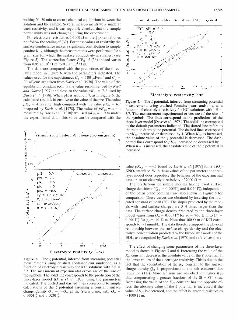
The data are compared with the predictions of the three-layer model in Figure 6, with the parameters indicated. Thevalues used for the capacitances C1 5 100 mF/cm2 and C2 520 mF/cm2 are taken from Davis et al. [1978]. The value of theequilibrium constant pK2 is the value recommended by Reviland Glover [1997] and close to the value pK2 5 7.2 used byDavis et al. [1978]. When pH is around 5.7, as in Figure 6, thecalculated result is insensitive to the value of the pzc. The valuepKK 5 4 is rather high compared with the value pKK 5 6.7proposed by Davis et al. [1978]. The value of pKCl was notmeasured by Davis et al. [1978]; we used pKCl 5 29 to matchthe experimental data. This value can be compared with the

value pKCl 5 24.5 found by Davis et al. [1978] for a TiO2-KNO3 interface. With these values of the parameter the three-layer model does reproduce the behavior of the experimentaldata up to an electrolyte resistivity of 2000 V m.

The predictions of simple models having fixed surfacecharge densities of Q0 5 0.005GS

0 and 0.020GS0 , independent

of the Stern plane potential, are also shown in Figure 6 forcomparison. These curves are obtained by inserting the indi-cated constant value in (30). The slopes predicted by the mod-els with fixed surface charges are 3–4 times larger than thedata. The surface charge density predicted by the three-layermodel varies from Q0 5 0.004GS

0 for r f 5 700 V m to Q0 50.001GS

0 for r f 5 10 V m. Note that 100 V m of KCl corre-sponds to ;1 mmol/L. The data therefore support the physicalrelationship between the surface charge density and the elec-trolyte concentration predicted by the three-layer model of theEDL, as recognized by Davis et al. [1978, and references there-in].

The effect of changing some parameters of the three-layermodel is shown in Figures 7 and 8. Increasing the value of theKK constant decreases the absolute value of the z potential atthe lower values of the electrolyte resistivity. This is due to thefact that the contribution of the KK constant to the surfacecharge density Q2 is proportional to the salt concentration(equation (11)). More K1 ions are adsorbed for higher KK,thus compensating a greater fractions of the Si 2 O2 sites.Increasing the value of the KCl constant has the opposite ef-fect: the absolute value of the z potential is increased if thevalue of KCl is decreased, and the effect is larger at resistivities;1000 V m.

Figure 6. The z potential, inferred from streaming potentialmeasurements using crushed Fontainebleau sandstone, as afunction of electrolyte resistivity for KCl solutions with pH 55.7. The measurement experimental errors are of the size ofthe symbols. The solid line corresponds to the prediction of thethree-layer model [Davis et al., 1978] using the parametersindicated. The dotted and dashed lines correspond to simplecalculations of the z potential assuming a constant surfacecharge density QS 5 2Q0 at the Stern plane, with Q0 50.005GS

0 and 0.020GS0 .

Figure 7. The z potential, inferred from streaming potentialmeasurements using crushed Fontainebleau sandstone, as afunction of electrolyte resistivity for KCl solutions with pH 55.7. The measurement experimental errors are of the size ofthe symbols. The lines correspond to the predictions of thethree-layer model [Davis et al., 1978]. The solid line correspondto the default parameters indicated. The dotted line refers tothe related Stern plane potential. The dashed lines correspondto pKK1 increased or decreased by 1. When KK1 is increased,the absolute value of the z potential is decreased. The dash-dotted lines correspond to pKCl increased or decreased by 1.When KCl is increased, the absolute value of the z potential isincreased.


The overall scale of the z potential is defined approximatelyby the product K2GS

0 (equation (9)), and the values of K andGS

0 are hard to determine independently from the data. In afirst approximation, using a higher value for the total surfacecharge site density is equivalent to increasing pK2.

The sensitivity of the theoretical prediction to the value ofthe s parameter is also shown in Figure 7, where the calculatedStern plane potential (dotted line) is compared with the zpotential (solid line). Using a nonzero s parameter introducesa small reduction of the absolute value of the z potential forsmall values of the electrolyte resistivity (20% at r f 5 100 Vm, 50% at r f 5 10 V m). This is due to the decrease of theDebye screening length when the ion concentration is in-creased (equation (29)). The Debye length for a solution ofKCl is ;10 nm/=c, where c is the KCl concentration inmmol/L. The effects of introducing a nonzero s parameter andof changing the values of the equilibrium constants are notexactly equivalent as a function of resistivity. However, thedata would also fit a model with s 5 0, a smaller value of theKCl parameter, and a larger value of the K2 equilibrium con-stant.

In Figure 8 the sensitivity of the prediction of the three-layerEDL model to the values of the capacitances C1 and C2 isillustrated. The z potential at pH 5 5.7 has little sensitivity tothe values of the capacitances.

For values of resistivity .5000 V m, however, the data showa smaller rate of increase with electrolyte resistivity, and thethree-layer model overestimates the data in this region. Thischange of slope at high resistivity was observed for almost allelectrolytes. For such high resistivities the concentration ofKCl is actually smaller than the concentrations of H1 andHCO3

2, and the properties of the EDL are actually controlledby the H1 and HCO3

2 ions. This fact is taken into account inthe theoretical curves shown in Figures 6 and 7 and is thus not

sufficient to explain the data, indicating that the chemical phe-nomena must be more complex in this region. The validity of(33) in this region is discussed by Lorne et al. [this issue].

In Figure 9 the experimental results are compared with theprediction of the simplified single-layer model [Revil andGlover, 1997] presented earlier in section 2.2 (see equation(19)). The values of the parameters indicated on Figure 9 areclose to the values recommended by Revil and Glover [1997].This simplified model explains the dependence of the z poten-tial as a function of the electrolyte resistivity about as well asthe three-layer model. In this model the surface charge densityfor pH , 7 can be approximated by (equation (19))

Q0~w0! 5 GS0

K2

cH10 exp S 2

w0

v0D , (38)

as the KCl and KK terms can be neglected. In the case of a 1:1electrolyte the Poisson-Boltzmann equation can be integratedanalytically, and (30) gives [Bard and Faulkner, 1980]

Q0~w0! 5 20.022 ÎcKCl sinh S w0

v0D e/nm2. (39)

When the concentration of KCl increases, the absolute value ofthe Stern plane potential decreases to maintain the equalitybetween (38) and (39). The physical origin of the resistivitydependence of the z potential is then the fact that the concen-tration of H1 ions on the mineral surface is increased forhigher absolute values of the Stern plane potential. Whenmore ions are present in the solution, the Stern plane electriccharge is screened more efficiently and a lower electric poten-tial develops (see equation (39)). However, this reduction isdamped by the fact that the enhancement of the H1 concen-tration on the mineral surface is less efficient, and hence moreSi 2 O2 species are produced by reaction (1) to maintain theequilibrium (equation (38)).

Figure 9. The z potential, inferred from streaming potentialmeasurements using crushed Fontainebleau sandstone, as afunction of electrolyte resistivity for KCl solutions with pH 55.7. The measurement experimental errors are of the size ofthe symbols. The lines correspond to the predictions of a sim-plified one-layer model [Revil and Glover, 1997]. The solid linecorresponds to the default parameters indicated. The dottedline refers to the related Stern plane potential.

Figure 8. The z potential, inferred from streaming potentialmeasurements using crushed Fontainebleau sandstone, as afunction of electrolyte resistivity for KCl solutions with pH 55.7. The measurement experimental errors are of the size ofthe symbols. The lines correspond to the predictions of thethree-layer model [Davis et al., 1978]. The solid line corre-sponds to the default parameters indicated. The dashed linecorresponds to a C1 capacitance twice as large. The dash-dotted line corresponds to a C2 capacitance twice as large.


4.3. Effect of pH

The z potential is shown as a function of pH for NaCl inFigure 10 and for KCl in Figure 11. For the data in Figure 10,pH was adjusted by adding HCl (pH , 5.7) or NaOH (pH .5.7) and the conductivity of the solution was adjusted by addingNaCl. In Figure 10, most measurements correspond to anelectrolyte resistivity of 100 V m; however, for pH , 3.3 andpH . 10.2 it was not possible to obtain the desired pH and tomaintain a resistivity of 100 V m. In Figure 11, pH was adjustedusing KOH instead of NaOH, and all measurements with KClwere performed with a solution resistivity of 25.5 V m.

In Figure 10 the change of sign of the z potential whencrossing the pzc is clearly observed. The value of the pzc ismeasured to be 2.5 6 0.1. The shape of the pH dependence isin good agreement with the measurements of Ishido and Mi-zutani [1981], Somasundaran and Kulkarni [1973], or Massenetand Pham [1985b]. The absolute value of the z potential re-ported by Ishido and Mizutani [1981], however, is 2–3 timeslarger. A pzc close to 4.5 was measured by Massenet and Pham[1985b] for volcanic ashes from Mount Etna. The value of thepzc depends on the minerals present in the sample [Ishido andMizutani, 1981]. Somasundaran and Kulkarni [1973] reported a

steeper variation with pH than observed in this experiment orby other workers.

For pH from 5.7 to 8, which is the domain for most appli-cations with natural groundwater, the observed variations areapproximately linear and can be represented by

zCFSNaCl~r f 5 100 V m, pH! 5 zCFS

NaCl~r f 5 100 V m, pH 5 5.7!

z @1 1 ~0.068 6 0.004!~pH 2 5.7!#(40a)

zCFSKCl ~r f 5 25 V m, pH! 5 zCFS

KCl ~r f 5 25 V m, pH 5 5.7!@1

1 ~0.14 6 0.02!~pH 2 5.7!] (40b)

The measurements are compared with the three-layer EDLmodel in Figures 10, 11, and 12. The three-layer model, withthe values of the parameters used in the previous discussion,accommodates well the experimental data. For NaCl, a valueof C1 5 70 mF/cm2 was used. In Figure 10 the model calcu-lation is sensitive to the values of the parameters, in particularfor pH close to pzc. If the value of the KNa constant is in-creased, the scale of the z potential is reduced, especially forincreasing pH, and the slope for pH . 6 is also reduced. Themodel prediction is most sensitive to the value of the KCl

constant for pH between pzc and 5. The model prediction maydeviate significantly from the experimental data if largechanges in the parameters are imposed, for example, by usingconstraints from other chemical data.

The Stern plane potential is also displayed in Figure 10, forthe indicated values of the parameters, to illustrate the effectof a nonzero s parameter. As shown previously by Ishido andMizutani [1981], the pH variation of the z potential is sensitive

Figure 10. The z potential, inferred from streaming potentialmeasurements using crushed Fontainebleau sandstone, as afunction of pH for NaCl/HCl/NaOH solutions. Diamonds cor-respond to measurements with an electrolyte resistivity of 100V m. Triangles correspond to measurements for which theelectrolyte resistivity is controlled by the pH and can not bemaintained at 100 V m. The measurement experimental errorsare of the size of the symbols. The lines correspond to thepredictions of the three-layer model [Davis et al., 1978]. Thesolid line corresponds to the default parameters indicated. Thedotted line refers to the related Stern plane potential. Thedashed lines correspond to pKNa increased or decreased by 1.When KNa is increased, the absolute value of the z potential isdecreased. The dash-dotted lines correspond to pKCl increasedor decreased by 1. When KCl is increased, the absolute value ofthe z potential is increased. The prediction from Ishido andMizutani [1981] is also shown for comparison (IM).

Figure 11. The z potential, inferred from streaming potentialmeasurements using crushed Fontainebleau sandstone, as afunction of pH for KCl/HCl/KOH solutions with a resistivity of25.5 V m. The measurement experimental errors are of the sizeof the symbols. The lines correspond to the predictions of thethree-layer model [Davis et al., 1978]. The solid line corre-sponds to the default parameters indicated. The dotted linerefers to the related Stern plane potential.


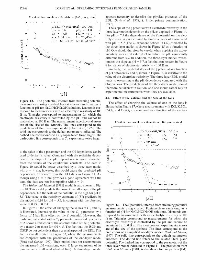
to the value of the s parameter, and the pH dependence can beused to derive its value. Compared with the resistivity depen-dence, the slope of the pH dependence is more decoupledfrom the values of the equilibrium constants. The data inFigure 10 would be better described by a three-layer modelwith s 5 4 nm; however, this would cause the predicted pHdependence to deviate from the KCl data in Figure 11. Al-though using s 5 2 nm provides a good agreement with thedata, the data are not incompatible with s 5 0.

The Ishido and Mizutani [1981] model is also shown in Fig-ure 10. This model predicts the correct overall shape of the pHdependence, but the scale of the potential is too high for pH .3.5. The value of the resistivity exponent of (37) predicted bythis model is 0.14 for pH 5 5.7, in contrast with the observedvalue of 0.23 6 0.014.

In Figure 12 the effect of changing the values of C1 and C2

is illustrated. Increasing the value of the C2 parameter by afactor of 2 has little effect on the z potential. However, thedash line, calculated with a C1 parameter increased by a factorof 2, shows a reduction of the absolute value of the z potentialby a factor 2 or more for pH , 5. The fact that the ISCP andOSCP do not coincide is then a crucial aspect of the EDL. Thisfact is also illustrated in Figure 13, where the measurementsare compared with the predictions of the one-layer model[Revil and Glover, 1997]. Their model does not accommodatethe measured pH variations, even if large excursions of itsparameters are allowed (dashed line). A three-layer model

appears necessary to describe the physical processes of theEDL [Davis et al., 1978; S. Pride, private communication,1997].

The slope of the z potential with electrolyte resistivity in thethree-layer model depends on the pH, as depicted in Figure 14.For pH 5 7.5 the dependence of the z potential on the elec-trolyte resistivity is increased by almost a factor of 2 comparedwith pH 5 5.7. The r f exponent defined in (37) predicted bythe three-layer model is shown in Figure 15 as a function ofpH. One should therefore be careful when applying the exper-imentally measured value 0.23 to values of pH significantlydifferent from 5.7. In addition, the three-layer model overes-timates the slope at pH 5 5.7, a fact that can be seen in Figure6 for values of electrolyte resistivity ,100 V m.

Similarly, the predicted slope of the z potential as a functionof pH between 5.7 and 8, shown in Figure 16, is sensitive to thevalue of the electrolyte resistivity. The three-layer EDL modeltends to overestimate the pH dependence compared with theobservations. The predictions of the three-layer model shouldtherefore be taken with caution, and one should rather rely onexperimental measurements when they are available.

4.4. Effect of the Valence and the Size of the Ions

The effect of changing the valence of one of the ions isillustrated in Figure 17, where measurements with KCl, K2SO4,CaCl2, and CaSO4 are compared as a function of the electro-

Figure 13. The z potential, inferred from streaming potentialmeasurements using crushed Fontainebleau sandstone, as afunction of pH for NaCl/HCl/NaOH solutions. Diamonds cor-respond to measurements with an electrolyte resistivity of 100V m. Triangles correspond to measurements for which theelectrolyte resistivity is controlled by the pH and cannot bemaintained at 100 V m. The measurement experimental errorsare of the size of the symbols. The lines correspond to thepredictions of a simplified one-layer model [Revil and Glover,1997]. The solid line corresponds to the default parametersindicated. The dotted line refers to the related Stern planepotential. The dashed line correspond to the parameters of thethree-layer model indicated in Figure 11. The prediction fromIshido and Mizutani [1981] is also shown for comparison (IM).

Figure 12. The z potential, inferred from streaming potentialmeasurements using crushed Fontainebleau sandstone, as afunction of pH for NaCl/HCl/NaOH solutions. Diamonds cor-respond to measurements with an electrolyte resistivity of 100V m. Triangles correspond to measurements for which theelectrolyte resistivity is controlled by the pH and cannot bemaintained at 100 V m. The measurement experimental errorsare of the size of the symbols. The lines correspond to thepredictions of the three-layer model [Davis et al., 1978]. Thesolid line corresponds to the default parameters indicated. Thedashed line corresponds to a C1 capacitance twice larger. Thedash-dotted line corresponds to a C2 capacitance twice larger.


lyte resistivity. Experiments using KCl were repeated, in be-tween these other salts, to check the reproducibility of thestreaming potential, and the pH was measured for each saltand for each value of streaming potential coefficient. The high-est resistivity (12,000 V m) is achieved using pure water, andthe coincidence of the data illustrates the excellent reproduc-ibility of the streaming potential measurements.

When even small quantities of salt are added to the solution,a greater reduction of the z potential is observed for divalentcations than for monovalent ions, as mentioned by Morgan etal. [1989] and Davis et al. [1978]. A divalent cation will indeedshield the negative charge of the EDL more efficiently.

Figure 14. The z potential, inferred from streaming potentialmeasurements using crushed Fontainebleau sandstone, as afunction of electrolyte resistivity for KCl solutions with pH 55.7. The measurement experimental errors are of the size ofthe symbols. The solid line corresponds to the prediction of thethree-layer model [Davis et al., 1978] using the parametersindicated. The dashed and dash-dotted lines correspond to thepredictions for pH 5 7.5 and pH 5 4.5, respectively.

Figure 15. The exponent parameter a as a function of pH,where a is defined as z 5 (r f)

a. The exponent is calculatedfrom 50 to 300 V m. The solid line corresponds to the predic-tion of the three-layer model [Davis et al., 1978] using theparameters indicated.

Figure 16. The relative variation of the absolute value of thez potential from pH 5 5.5 to pH 5 8, as a function of theelectrolyte resistivity. The solid line corresponds to the predic-tion of the three-layer model [Davis et al., 1978] using theparameters indicated.

Figure 17. The z potential, inferred from streaming potentialmeasurements using crushed Fontainebleau sandstone, as afunction of electrolyte resistivity for several salt solutions withpH 5 5.7, changing the valence of the ions. The lines corre-spond to the predictions of the three-layer model [Davis et al.,1978] with the parameters indicated in Table 1, from top tobottom KCl, K2SO4, CaCl2, and CaSO4.


Let us define the ratio of the z potential for a given solutionto the z potential for KCl at the same resistivity as the stream-ing potential chemical efficiency, noted ES. It can be seen inFigure 18 that the experimental values of the chemical effi-ciency are almost independent of the electrolyte resistivityfrom 40 to 2000 V m, in contrast with what can be inferredfrom earlier results [Morgan et al., 1989]. The experimentalvalues, listed in Table 1, cluster around 1 for monovalent ionsand 0.5 for divalent cations.

The accommodation of divalent cations in the three-layertheory is not straightforward. The curves shown in Figure 17have been calculated assuming the following adsorption reac-tions [Davis et al., 1978]:

Si 2 OH 1 Mn1 ¢O¡KM

Si 2 O 2 M1~n21! 1 H1, (41)

Si 2 OH 1 An2 1 H1 ¢O¡KA

Si 2 A~n21!2 1 H2O. (42)

and neglecting other types of complexation. For example, adivalent cation could, in principle, also make a complex withtwo Si 2 O2 sites [Davis et al., 1978].

Considering only the simple complexations of (41) and (42),the surface charge density Q2 (equation (7)) becomes

Q2 5 OX

zXGSi2X. (43)

In Figure 19 the effect of changing the nature of the ion whilekeeping a fixed valence is studied for monovalent ions (Li1,Na1, K1), and divalent ions (Mg21, Ca21, Ba21). In Figure 20,Na1 and K1 are compared when combined with Cl2 or NO3

2.In Figure 19 the z potential for Na1 is consistently smaller thanfor Li1 and K1, which are identical within the experimentalaccuracy. This effect is apparently not related to the actualionic radius, as the size of the lithium ion is about half the sizeof the potassium ion [Marcus, 1988] or to the Stokes solvatedradius which defines the ion mobility, as the mobilities oflithium and potassium are also different. For the divalent cat-ions the observed z potentials are ordered according to ionicsize, z(Mg) . z(Ca) . z(Ba).

In Figures 17 and 18 and in Table 1 it is possible to findvalues for the equilibrium constants so that the general fea-tures of the data are accommodated by the three-layer model,as indicated in the figure captions and in Table 1. However, thedetailed variations of the chemical efficiency with the electro-lyte resistivity do not agree well with the data (Figure 18),

Table 1. Streaming Potential Chemical Efficiencies ES forVarious Salts

Salt ES measured

ES calculatedr f 5 100 V m

pKK 5 4, pKCl 5 29

Monovalent IonsNaCl 0.930 6 0.003 0.933

(pKNa 5 4)KNO3 1.122 6 0.004 1.12

(pKNO35 29.5)

NaNO3 0.995 6 0.004 1.04pKNa 5 4, pKNO3

5 29.5

Monovalent Cation With Divalent AnionK2SO4 0.937 6 0.002 0.927

(pKSO45 27.5)

Li2CO3 0.882 6 0.003 0.88(pKLi 5 1.2), pKCO3

5 27.4Na2CO3 0.836 6 0.003 0.877

pKNa 5 4, pKCO35 27.4

K2CO3 0.889 6 0.003 0.893(pKCO3

5 27.4)

Divalent Cation With Monovalent AnionMgCl2 0.457 6 0.003 0.43

(pKMg 5 5.1)CaCl2 0.517 6 0.002 0.525

(pKCa 5 5.1)BaCl2 0.552 6 0.002 0.56

(pKBa 5 5.3)

Divalent IonsCaSO4 0.494 6 0.003 0.577

pKCa 5 5.1, pKSO45 27.5

Trivalent CationTl(NO3)3 0.377 6 0.006 0.32

(pKTl 5 5.6), pKNO35 29.5

The reference is KCl. Most measurements are performed at pH 55.7, except for the carbonates for which pH 5 8. The experimentalvalue is the average of the measurements from 40 to 2000 V m. Thepredictions of the three-layer EDL model correspond to the indicatedvalues of the equilibrium constants and are given for an electrolyteresistivity of 100 V m. The equilibrium constants indicated in paren-theses are chosen so that the prediction is matching the experimentalvalue. When the equilibrium constants are not in parentheses, it meansthat the theoretical predictions is constrained by other measurements,and the comparison with the data is meaningful.

Figure 18. The streaming potential chemical efficiency as afunction of electrolyte resistivity for several salt solutions withpH 5 5.7. The measurement experimental errors are of thesize of the symbols. The lines correspond to the predictions ofthe three-layer model [Davis et al., 1978] with the parametersindicated in Table 1, from top to bottom K2SO4, CaCl2,CaSO4, and Tl(NO3)3.


indicating that a more refined understanding of the surfacechemistry is necessary.

Chemical efficiency depends in part on the mobility of theions, which for the various ions imposes different ion concen-trations for a given electrolyte resistivity. This effect is takeninto account in our calculation and accounts for the observeddifference between KCl and NaCl (see Table 1), at least at 100V m.

Interestingly, the change of slope of z potential as a functionof electrolyte resistivity observed for all other ions for electro-lyte resistivity .1000 V m is not observed for carbonates (Fig-ure 19). The carbonates show a linear variation over the wholerange of resistivity up to the maximum value corresponding topure distilled water. This may indicate that salt adsorption,taking place on the quartz surface, is affected by the presenceof dissolved carbonate from the atmospheric CO2. This effectwould not be observed when the solution provides enoughHCO3

2 ions from the salt.Data for trivalent ions are presented in Figures 18 and 20.

The chemical efficiency for Tl31 is stable for electrolyte resis-tivity ,2000 V m (Figure 18) and amounts to ;0.38 (Table 1),indicating that chemical efficiency seems to be close to theinverse of the valence of the cation. This empirical observation,however, is not supported by the three-layer model, in whichthe value of the chemical efficiency essentially results from thevalues of the adsorption constants and does not scale as l/zC.

The z potential for Al31 (Figure 20) decreases to almost

zero for resistivities ,1000 V m. The sharp decrease of thepotential when small amounts of aluminum nitrate are addedagain points to the importance of additional chemical reactionstaking place on the quartz surface, as already mentioned byMorgan et al. [1989] and Ishido and Mizutani [1981]. The pres-ence of traces of Al31 ions in the Fontainebleau samples mayalso explain the reduction of z potential with respect to pre-dictions for high resistivity [Rasmusson and Wall, 1997; A.Revil, private communication, 1997]. Taking pKA1

5 3.7, theprediction from the three-layer model is in good agreementwith the data (Table 1 and Figure 20).

4.5. Effect of Grain Size or Permeability

The inferred values of the z potential (using equation (33)and the experimental values of the streaming potentials) areshown in Figure 21 for several grain sizes as a function of themeasured permeability. A variation of the z potential withpermeability or grain size could be due to the presence ofsurface conductivity, as suggested by (33). The effect of typicalpore size on the electrical structure of the EDL can be con-sidered negligible [Pride and Morgan, 1991], as shown in theappendix.

In order to illustrate the role of the surface conductivity, twodata sets are shown in Figure 21 with KCl, one for an electro-lyte resistivity of 1000 V m and pH 5 5.7 and one for anelectrolyte resistivity of 400 V m and pH 5 7. In order to beable to compare the two data sets the data set for 1000 V m

Figure 19. The z potential, inferred from streaming potentialmeasurements using crushed Fontainebleau sandstone, as afunction of electrolyte resistivity for several salt solutions withpH 5 5.7 for chloride ions and pH varying between 7 and 8 forthe carbonates. The results for several ions with the samevalence but different natures are compared. The solid linescorrespond to the predictions of the three-layer model [Daviset al., 1978] for K2CO3 and CaCl2. The dotted lines correspondto a pKcat parameter increased by 1. The dashed lines corre-spond to a C1 capacitance twice as large.

Figure 20. The z potential, inferred from streaming potentialmeasurements using crushed Fontainebleau sandstone, as afunction of electrolyte resistivity for several salt solutions withpH 5 5.7. The results for Na1 and K1 are compared for twoanions, and two examples of trivalent ions are given. The linescorrespond to the predictions of the three-layer model [Daviset al., 1978], from top to bottom KCl, Tl(NO3)3, and Al(NO3)3.The inferred values of the equilibrium constants are pKTl 55.6 (Table 1) and pKAl 5 3.7.


and pH 5 5.7 was transferred to the conditions of the data setwith 400 V m and pH 5 7 using the experimentally determinedrelations (37) and (40).

Smaller potentials are observed for permeability smallerthan 5 darcies (grain sizes ,150 mm). This reduction of zpotential, which is more important for the data sample mea-sured at r f 5 1000 V m, illustrates the fact that for smallergrain sizes the contribution of surface conductivity can not beneglected.

In Figure 21b our data show that a surface conductivitymodel of 0.17 mS/m at low permeability, 0.01 at high perme-ability and a smooth transition at 5 darcies, and a bulk forma-tion factor F0 which follow a scaling law k20.09, is consistentwith the measurements. If the surface conductivity is thustaken into account using this model and (33), as in Figure 21a(bottom), the corrected z potential is roughly independent ofthe permeability for permeability ,5 darcies. Also, measure-ments with different electrolyte resistivity agree, as the F/F0

correction in (33) increases with increasing electrolyte resistivity.For permeability larger than 50 darcies a sharp drop in

streaming potential is observed in Figure 21a. To check thereproducibility of this observation, the z potential for two highvalues of permeability was measured using a different experi-mental setup in which the differential pressure across the sam-ple was measured directly from the height of water in verticalglass tubes in order to be independent from head loss correc-tions. Although slightly higher than the other data, these twomeasurements confirm the drop at high permeability. A de-

crease of the streaming potential for large grain sizes was alsonoted by Ahmad [1964], although of smaller magnitude. Forsuch large values of permeability, flow rate and turbulenceeffects might become important, although the deviation of thestreaming coupling coefficient from linearity was not found tobe large (Figure 4). For such flow rates, however, the size ofthe noncirculating electrolyte volumes in the sample may be ofthe order of magnitude of the grain size. More studies need tobe performed to understand this effect, which may be impor-tant in some geophysical systems like fault zones. We expandfurther on the fact that the z potential is essentially constantbetween 10 mdarcy to 10 darcies in the companion paper byLorne et al. [this issue].

5. Applications to Natural Geophysical Systems5.1. Streaming Potentials for Various Rock Minerals

In order to extrapolate the results obtained in the laboratoryto geophysical field conditions, the effects of different mineralsand fluid chemistry must be addressed. Results of the mea-surement of the z potential for various crushed rocks are pre-sented in Table 2. Rocks samples are crushed, and the grainsare selected by sieving so that the resulting permeability in theexperimental assembly is of the order of a few darcies at most.Crystalline and calcareous rocks are included, together with asample of all major rock types present in a typical field site inthe Alps, at the geological contact between the Belledonecrystalline belt and the Mesozoic layers [Perrier et al., 1998;Trique et al., 1999].

For granite a z potential of 252 6 1 mV is inferred for anelectrolyte resistivity of 350 V m and pH 5 7, compatible withresults obtained for Westerly granite [Morgan et al., 1989]. Formost rocks the z potentials tend to be much smaller than the

Figure 21a. The z potential, inferred from streaming poten-tial measurements using crushed Fontainebleau sandstone, asa function of the sample permeability. The diamonds corre-spond to a KCl solution of 400 V m resistivity and pH 5 7, andthe triangles correspond to another crushed sample with a KClsolution of 1000 V m resistivity and pH 5 5.7. The squarescorrespond to measurements with another experimental setup(see text). The results are compared with and without takinginto account the effect of the surface conductivity on thestreaming potential coefficient in equation (37).

Figure 21b. Surface conductivity and bulk formation factoras a function of permeability. The three experimental measure-ments are compared with the ad hoc model (solid line) de-scribed in the text and used to correct for surface conductivityin Figure 21a.


results obtained for Fontainebleau sandstone. The results forseveral types of sandstone can be quite different. Increasingthe number of mineral phases tends to reduce the z potentialsignificantly. For limestones the electrolyte always contains asignificant concentration of dissolved calcium and magnesium,which reduces the z potential as shown in section 4.

5.2. Streaming Potentials With Real Natural Water

Natural aqueous solutions are quite different from purewater with dissolved KCl, and the resistivity is rarely .400 Vm, except for pure rain water (.1000 V m, although lower inindustrial areas) and melted snow water in mountainous areas(for example, we measured about 1600 V m in the FrenchAlps). In marine systems the resistivity of seawater is ,0.2 V m(resistivity corresponding to the NaCl concentration at satura-tion) and the observation of streaming potentials in such en-vironments is difficult. In a continental geophysical system, theresistivity of freshwater lakes varies around an average value of;50 V m (value measured by the authors in lakes in the FrenchAlps). For spring water the resistivity varies between 26 V mfor a carbonate formation and 350 V m for a crystalline for-mation. The pH in general is close to 7 but can reach values aslow as 6 for crystalline waters [Probst et al., 1992] and as highas 8 for some carbonated waters [Sigg et al., 1992].

The z potential was inferred for some mineral waters withone sample of crushed Fontainebleau sandstone from the mea-sured streaming potentials using (33). The results are compiledin Table 3. The streaming potential chemical efficiency ES hasbeen calculated using (37) and (40).

The chemical efficiency is 0.44 6 0.05 for the limestonewater. This solution was obtained from crushed KimmeridgianGarchy limestone at the edge of the Parisian basin. Its char-acteristics are similar to the parameters of a theoretical opencalcite system in equilibrium with water and the atmosphere[Sigg et al., 1992]. The z potential of this system increases withincreasing pH (Figure 10), but the conductivity and the chem-ical efficiency are low. For a closed system, where pore water

is not in contact with the atmosphere, the pH is high (pH 59.9) and the concentrations of dissolved ions reduced; there-fore the water resistivity is also higher.

Two measurements were performed with commercial min-eral water. The St. Lambert water is one example of a naturallystrongly carbonated water, but the measured chemical effi-ciency (Table 3) is high (0.8). This is in contradiction with theprevious measurement with limestone water (ES 5 0.44 60.05), suggesting that calcium carbonate has precipitated. TheVolvic water is less conductive than the St. Lambert water andhas a smaller dissolved carbonate content, a slightly higher zpotential, and a similar chemical efficiency.

The chemical efficiency can also be calculated using thethree-layer numerical model presented before. The values aregiven in Table 3 and are generally consistent with the mea-surements, except for the St. Lambert water and water typicalof a crystalline environment [Probst et al., 1992], which was notmeasured. This last example illustrates the higher resistivity ofwater in such areas. In conclusion, the chemical efficiency formineral waters is ;80%, except for strongly carbonated watersfor which it can be as low as 40%. In order to estimate the zpotential in a given environment these efficiencies have to beapplied to the values of the z potentials given in Table 2,according to the dominating mineralogy, and applying the scal-ing laws (37) and (40) for water resistivity and pH, respectively.

In order to estimate the streaming potential coefficient, theeffect of the rock permeability must be understood, and this isthe topic of the companion paper. The experimentally deter-mined scaling laws can be used to estimate the streamingpotential change that would be induced by a geochemicalchange. The relative potential variation d12 that would be as-sociated with a change of chemical conditions would be pro-portional to

d12 5~r f!2z2 2 ~r f!1z1

~r f!1z1, (44)

where the subscript 1 refers to the initial conditions.

Table 2. The z Potential for Various Rocks Measured With a Solution of KCl WithpH 5 5.7 for All Rocks Except for Limestones for Which the pH is 8

Rock Mineralogy

ElectrolyteResistivity,

V mz Potential,

mV

Igneous and Metamorphic RocksGranodiorite 350 252 6 1Paragneiss (Alps) clay/carbonate cement 312 226 6 0.5Basalt (Pacific islands) aluminosilicates 188 218 6 0.4

Sedimentary Rocks With QuartzFontainebleau sandstone 99% quartz 400 240 6 5Vosges sandstone quartz with hematite traces 80 216 6 0.3Permian sandstone (Alps) quartz 1 carbonates 300 28.6 6 0.2Houiller sandstone (Alps) quartz with anthracite and

clay beds400 212 6 0.2

Trias quartzite quartz 400 27.1 6 0.1Bajocian schist 295 29.3 6 0.2

Carbonated RocksCallovo-oxfordian limestone 311 25 6 0.2Kimmeridgian limestone (Alps) calcite with clay 300 21.2 6 0.2Coral reef (Pacific island) aragonite 200 24.3 6 0.2Cellular dolomite (Alps) dolomite 278 24.2 6 0.1

Electrolytes for limestones also include a significant content of dissolved carbonates. The indicatedexperimental errors correspond to the experimental error of a single measurement, except in the case ofFontainebleau sandstone where the sample to sample dispersion is taken into account.


For example, before the Kobe earthquake, geochemicalchanges were observed in the ground water [Tsunogai andWakita, 1995]. In particular, an increase of 10% in the concen-tration of chloride ions, correlated to an increase of 30% ofsulfate ions, was observed. A similar phenomenon was ob-served before an earthquake in the French Pyrenees [Toutainet al., 1997]. Taking the typical composition of a water in acrystalline area given by Probst et al. [1992], one can estimatethe d12 factor as 210% for such a change of water chemistry,using the results from Table 3 and our three-layer numericalmodel. If we imagine a situation in which the electric potentialis being monitored at two locations of an aquifer with a dipolelength of 500 m or more, it is not unwarranted to expect toobserve a static electric potential difference of ;100 mV at thebottom of piezometers, associated with the discharge flow ofthe aquifer. The above change in chemical conditions, withoutany change in the dynamics of the discharge, would produce anelectrical signal of ;10 mV, which is larger than the drift noiseof the electrodes and their installation schemes [Perrier et al.,1997]. Such a slowly varying precursory electrical signal wouldthen be observable in association with geochemical changesbefore earthquakes.

6. ConclusionsIn this paper a systematic study of the z potential inferred

from streaming potential measurements with crushed Fon-tainebleau sandstone is presented as a function of the electro-lyte resistivity, pH, and ionic composition. The z potential wasalso inferred from streaming potential measurements usingother rock types and natural groundwaters. The goal of thesemeasurements is to improve our understanding of the physicsof the electrical double layer. Various empirical laws werederived from the measurements which can be used for estimat-ing streaming potential effects in geophysical systems, as illus-trated by Perrier et al. [1998, 1999].

The results were compared with the predictions of a three-layer EDL numerical model [Davis et al., 1978]. This modelaccounts for the general features of the data and allows valuesof the equilibrium constants of the adsorption reactions andthe spatial structure of the EDL to be determined from thedata. Variations of the z potential with pH can not be ac-counted for by a single-layer model but are generally predictedby the three-layer model; however, the details of the measuredz potential variations as a function of electrolyte resistivity for

Table 3. The z Potential and the Streaming Potential Chemical Efficiencies ES for SomeNatural Waters Measured With Crushed Fontainebleau Sandstone

Electrolyte pH

ElectrolyteResistivity,

V m z, mV

ES

Measured Calculated

KCl 5.5 390 247 1 1Calcite open system 8.3 (148) (0.34)

[Sigg et al., 1992]cHCO32 5 0.907cCa21 5 0.454

Calcite closed system 9.9 (331) (0.39)[Sigg et al., 1992]cHCO32 5 0.081cCO322 5 0.033cCa21 5 0.114

Limestone solution(solution inequilibrium withKimmeridgianlimestone)

9.0 175 220.2 0.44 6 0.05 (0.34)

St. Lambert mineralwater

7.2 24.6 221.8 0.81 6 0.08 (0.28)

cCa21 5 1.58cMg21 5 0.31cNa1 5 0.71cK1 5 0.03cCl2 5 0.79cSO422 5 0.26

Volvic mineral water 7.0 66 226.0 0.77 6 0.08 (0.59)cCa21 5 0.22cMg21 5 0.21cNa1 5 0.44cK1 5 0.15cCl2 5 0.34cSO422 5 0.08

Vosges spring water 6.1 (125) (0.58)[Probst et al., 1992]cCa21 5 0.19cMg21 5 0.06cNa1 5 0.08cK1 5 0.02cCl2 5 0.06cSO422 5 0.21

Calculated numbers in parentheses are obtained using the three-layer EDL numerical model. Concen-trations are expressed in mmol/L.


various types of ions are not well reproduced. More input fromsurface chemistry may be useful in assessing reasonable valuesfor the parameters of the three-layer model. Also, the values ofthe equilibrium constants given in this paper are correlatedwith other parameters, and it may be hazardous to translatethese values to other contexts. In any case, as illustrated by thecomparisons presented in the figures, the data presented in thispaper can be used to improve our theoretical understanding ofthe EDL.

AppendixA1. Effect of Crack Size

The effect of a finite size crack can be studied by using aslight modification of (28). Indeed, the integration of the Pois-son-Boltzmann equation (27) can be performed from 0 to afinite position d , where the derivative dw/dx 5 0 is 0. This is,for example, the case for a crack of half width d separating twoparallel planar rock surfaces. The first-order differential equa-tion for the potential is then, instead of (28),

dw

dx 5 2sign ~QS!v0

xd

z ÎOi

c i0F exp S22zi

w

v0D 2 exp S22zi

wd

v0D G

2 Oi

z i2ci

0 , (A1)

where wd is the value of the potential in the center of the crack.Equation (A1), combined with the boundary condition (30),can be solved numerically, starting from some value of wd anditerating until the new boundary condition dw/dx 5 0 for x 5d is met within a preset precision. The results are shown inFigure A1 for a single-layer EDL model and a constant surfacecharge on the Stern plane. One can see that decreasing theaperture of a finite crack size increases the value of the Stern

plane potential, and consequently the value of the z potential,for a fixed s parameter. However, this effect is very small,unless extremely small crack sizes are considered. The typicalsize of a pore in a Fontainebleau sandstone is ;150 mm, withthroats of the order of 1 mm. The effect is larger for higherelectrolyte resistivities, as illustrated in Figure A2a but remainsvery small. The finite size of cracks is neglected in our datainterpretation.

A2. Effect of Ion-Ion Interactions

The interaction between ions can result in charge shieldingfor concentrated solutions. This may have a significant effect ofthe z potential, which is sensitive to the charge distribution ofthe ions. This effect was estimated using the Debye-Huckeltheory of ionic activities [Bard and Faulkner, 1980]. Activitycoefficients g given by

log g 5 20.509 Î1023 ci0 exp F22zi

w

v0G , (A2)

were inserted in the Poisson-Boltzmann equation, which wasthen numerically integrated. In (A2) the effect is overesti-mated in order to take into account the fact that both cationand anion activities increase near the surface compared withthe free electrolyte. The result is shown in Figure A2b. Thecalculated effect on the z potential is ,1%. Ion-ion electro-

Figure A1. The z potential as a function of crack width, for aquartz-KCl solution interface, calculated using a simple one-layer model assuming a constant surface charge density on theStern plane.

Figure A2. (a) The z potential as a function of electrolyteresistivity for an infinitely large crack (solid line) and a crackwith a 20 nm half width (dotted line). (b) The effect on the zpotential of including ion activity coefficients in the numericalintegration of the Poisson-Boltzmann equation. The scatter ofpoints reflects the accuracy of the numerical calculation.


static interactions can therefore be neglected in our study evenfor electrolyte resistivities ,10 V m. Ion-ion interactions donot explain the discrepancies between the data and some the-oretical calculations.

Acknowledgments. The authors are grateful to the Laboratoire deDetection et de Geophysique for financial and technical support.Funds were also received from the French Ministry of Environment.Most of the experiments were performed with the help of ThierryFroidefond and Pierre Lalance. In addition, Jean Aupiais and his teamof chemists helped with advise, equipment, measurements, and anal-ysis of the electrolytes. Patrick Dupont is thanked for the fabrication ofmany pieces of the apparatus. The authors also acknowledge enlight-ening exchanges with Laurence Jouniaux, Jean-Pierre Pozzi, PaulGlover, and Andre Revil and especially thank Steve Pride for intro-ducing them to the work of Davis et al. [1978]). M. Johnston and B. J.Wanamaker are thanked for their detailed and constructive review.

ReferencesAhmad, M. U., A laboratory study of streaming potentials, Geophys.

Prospect., 12, 49–64, 1964.Antraygues, P., and M. Aubert, Self potential generated by two-phase

flow in a porous medium: Experimental study and volcanologicalapplications, J. Geophys. Res., 98, 22,273–22,281, 1993.

Bard, A. J., and L. R. Faulkner, Electrochemical Methods, Fundamen-tals and Applications, John Wiley, New York, 1980.

Bernard, P., Plausibility of long distance electrotelluric precursors toearthquakes, J. Geophys. Res., 97, 17,531–17,546, 1992.

Bikerman, J. J., Electrokinetic potentials, in The Encyclopedia of Elec-trochemistry, edited by C. A. Hampel, pp. 471–475, Reinhold, NewYork, 1964.

Bogoslovsky, V. A., and A. A. Ogilvy, Natural potential anomalies asa quantitative index of the rate of seepage from water reservoirs,Geophys. Prospect., 18, 261–268, 1970.

Bogoslovsky, V. A., and A. A. Ogilvy, The study of streaming poten-tials on fissured media models, Geophys. Prospect., 20, 109–117,1972.

Byerlee, J. D., Friction, overpressure and fault normal compression,Geophys. Res. Lett., 17, 2109–2112, 1990.

Chandler, R., Transient streaming potential measurements on fluid-saturated porous structures: An experimental verification of Biot’sslow wave in the quasi-static limit, J. Acoust. Soc. Am., 70, 116–121,1981.

Corwin, R. F., and D. B. Hoover, The self-potential method in geo-thermal exploration, Geophysics, 44, 226–245, 1979.

David, C., Geometry of flow paths for fluid transport in rocks, J.Geophys. Res., 98, 12,267–12,278, 1993.

Davis, J. A., R. O. James, and J. O. Leckie, Surface ionization andcomplexation at the oxide/water interface, J. Colloid Interface Sci.,63, 480–499, 1978.

Ernstson, K., and H. U. Scherer, Self-potential variations with timeand their relation to hydrogeologic and meteorological parameters,Geophysics, 51, 1967–1977, 1986.

Fenoglio, M. A., M. J. S. Johnston, and J. D. Byerlee, Magnetic andelectric fields associated with changes in high pore pressure in faultzones: Applications to the Loma Prieta ULF emissions, J. Geophys.Res., 100, 12,951–12,958, 1995.

Fujinawa, Y., T. Kumagai, and K. Takahashi, A study of anomalousunderground electric field variations associated with a volcanic erup-tion, Geophys. Res. Lett., 19, 9–12, 1992.

Glover, P. W. J., P. G. Meredith, P. R. Sammonds, and S. A. F. Murell,Ionic surface conductivity in sandstone, J. Geophys. Res., 99, 21,635–21,650, 1994.

Hashimoto, T., and Y. Tanaka, A large self-potential anomaly onUnzen volcano, Shimabara peninsula, Kyushu island, Japan, Geo-phys. Res. Lett., 22, 191–194, 1995.

Iler, R. K., The Chemistry of Silica, John Wiley, New York, 1979.Ishido, T., and H. Mizutani, Experimental and theoretical basis of

electrokinetic phenomena in rock-water systems and its applicationsto geophysics, J. Geophys. Res., 86, 1763–1775, 1981.

Johnson, P. A., and T. V. McEvilly, Parkfield seismicity: Fluid-driven?,J. Geophys. Res., 100, 12,937–12,950, 1995.

Jouniaux, L., and J. P. Pozzi, Permeability dependence of streaming

potential in rocks for various fluid conductivities, Geophys. Res. Lett.,22, 485–488, 1995a.

Jouniaux, L., and J. P. Pozzi, Streaming potential and permeability ofsaturated sandstones under triaxial stress: Consequences for elec-trotelluric anomalies prior to earthquakes, J. Geophys. Res., 100,10,197–10,209, 1995b.

Jouniaux, L., and J. P. Pozzi, Laboratory measurements anomalous0.1–0.5 Hz streaming potential under geochemical changes: Impli-cations for electrotelluric precursors to earthquakes, J. Geophys.Res., 102, 15,335–15,343, 1997.

Lorne, B., F. Perrier, and J. P. Avouac, Streaming potential measure-ments, 2, Relationship between electrical and hydraulic flow pat-terns from rock samples during deformation, J. Geophys. Res., thisissue.

Malengreau, B., J. F. Lenat, and A. Bonneville, Cartography andtemporal observation of self-potential (SP) anomalies at Piton de laFournaise, Bull. Soc. Geol. Fr., 165, 221–232, 1994.

Marcus, Y., Ionic radii in aqueous solutions, Chem. Rev., 88, 1475–1498, 1988.

Massenet, F., and V. N. Pham, Mapping and surveillance of activefissure zones on a volcano by the self-potential method, Etna, Sicily,J. Volcanol. Geotherm. Res., 24, 315–338, 1985a.

Massenet, F., and V. N. Pham, Experimental and theoretical basis ofself-potential phenomena in volcanic areas with reference to resultsobtained on Mount Etna (Sicily), Earth Planet. Sci. Lett., 73, 415–429, 1985b.

Michel, S., and J. Zlotnicki, Self-potential and magnetic surveying ofLa Fournaise volcano (Reunion Island): Correlations with faulting,fluid circulation, and eruption, J. Geophys. Res., 103, 17,845–17,857,1998.

Mizutani, H., T. Ishido, T. Yokotura, and S. Ohnishi, Electrokineticphenomena associated with earthquakes, Geophys. Res. Lett., 3, 365–368, 1976.

Morat, P., and J. L. Le Mouel, Electrical signals generated by thecollapse of the pillars of a gypsum quarry, C. R. Acad. Sci., Ser. II,308, 33–38, 1989.

Morat, P., and J. L. Le Mouel, Electrical signals generated by stressvariations in porous non saturated rocks, C. R. Acad. Sci., Ser. II,315, 955–963, 1992.

Morgan, F. D., E. R. Williams, and T. R. Madden, Streaming potentialproperties of Westerly granite with applications, J. Geophys. Res., 94,12,449–12,461, 1989.

Muir-Wood, R., and G. C. P. King, Hydrological signatures of earth-quake strain, J. Geophys. Res., 98, 22,035–22,068, 1993.

Nur, A., and J. R. Booker, Aftershocks caused by fluid flow, Science,175, 885–887, 1972.

Ogilvy, A. A., M. A. Ayed, and V. A. Bogoslovsky, Geophysical studiesof water leakages from reservoirs, Geophys. Prospect., 17, 36–62,1969.

Overbeek, J. T., Colloid Science, edited by H. R. Kruyt, Elsevier, NewYork, 1960.

Park, S. K., M. J. S. Johnston, T. R. Madden, and H. F. Morrison,Electromagnetic precursors to earthquakes in the ULF band: Areview of observations and mechanisms, Rev. Geophys., 31, 117–132,1993.

Perrier, F., et al., A one-year systematic study of electrodes for longperiod measurement of the electric field in geophysical environ-ments, J. Geomagn. Geoelectr., 49, 1677–1696, 1997.

Perrier, F., M. Trique, B. Lorne, J. P. Avouac, S. Hautot, and P. Tarits,Electric potential variations associated with lake level variations,Geophys. Res. Lett., 25, 1955–1958, 1998.

Perrier, F., M. Trique, J. Aupiais, U. Gautam, and P. Shrestha, Electricpotential variations associated with periodic spring discharge inwestern Nepal, C. R. Acad. Sci., Ser. II, 328, 73–79, 1999.

Pisarenko, D., P. Morat, and J. L. Le Mouel, On a possible mechanismof sandstone alteration: Evidence from electric potential measure-ments, C. R. Acad. Sci., Ser. II, 322, 17–24, 1996.

Pride, S., Governing equations for the coupled electromagnetics andacoustics of porous media, Phys. Rev. B Condens. Matter, 50, 15,678–15,696, 1994.

Pride, S. R., and F. D. Morgan, Electrokinetic dissipation induced byseismic waves, Geophysics, 56, 914–925, 1991.

Probst, A., D. Viville, B. Fritz, B. Ambroise, and E. Dambrine, Hy-drochemical budgets of a small forested granitic catchment exposedto acid deposition: The Strengbach catchment case study (Vosgesmassif, France), Water Air Soil Pollut., 62, 337–347, 1992.


Rasmusson, M., and S. Wall, Electrostatic characterisation of Al-modified, nanosized silica particles, Colloids Surf. A, 122, 169–181,1997.

Revil, A., and P. W. J. Glover, Theory of ionic-surface electrical con-duction in porous media, Phys. Rev. B Condens. Matter, 55, 1757–1773, 1997.

Ruffet, C., Y. Gueguen, and M. Darot, Complex conductivity mea-surements and fractal nature of porosity, Geophysics, 56, 758–768,1991.

Scholz, C. H., L. R. Sykes, and Y. P. Aggarwal, Earthquake prediction:A physical basis, Science, 181, 803–810, 1973.

Sigg, L., W. Stumm, and P. Behra, Chimie des Milieux Aquatiques,Masson, Paris, 1992.

Sleep, N. H., and M. L. Blanpied, Creep, compaction and the weakrheology of major faults, Nature, 359, 687–692, 1992.

Somasundaran, P., and R. D. Kulkarni, A new streaming potentialapparatus and study of temperature effects using it, J. Colloid Inter-face Sci., 45, 591–600, 1973.

Sprunt, E. S., T. B. Mercer, and N. F. Djabbarah, Streaming potentialfrom multiphase flow, Geophysics, 59, 707–711, 1994.

Toutain, J. P., M. Munoz, F. Poitrasson, and A. C. Lienard, Spring-water chloride ion anomaly prior to an ML 5 5.2 Pyrenean earth-quake, Earth Planet. Sci. Lett., 149, 113–119, 1997.

Trique, M., P. Richon, F. Perrier, J. P. Avouac, and J. C. Sabroux,Radon emanation and electric potential variations associated withtransient deformation in the vicinity of reservoir lakes, Nature, 399,137–141, 1999.

Tsunogai, U., and H. Wakita, Precursory chemical changes in groundwater: Kobe earthquake, Japan, Science, 269, 61–63, 1995.

Wurmstich, B., and F. D. Morgan, Modeling of streaming potentialresponses caused by oil well pumping, Geophysics, 59, 46–56, 1994.

Yoshida, S., M. Uyeshima, and M. Nakatani, Electric potentialchanges associated with slip failure of granite: Preseismic and co-seismic signals, J. Geophys. Res., 102, 14,883–14,897, 1997.

Zlotnicki, J., and J. L. Le Mouel, Volcanomagnetic effects observed onPiton de la Fournaise volcano (Reunion Island): 1985–1987, J. Geo-phys. Res., 93, 9157–9171, 1988.

Zlotnicki, J., and J. L. Le Mouel, Possible electrokinetic origin of largemagnetic variations at La Fournaise Volcanoe, Nature, 343, 633–636, 1990.

Zlotnicki, J., S. Michel, and C. Annen, Anomalies de polarisationspontanee et systemes convectifs sur le volcan du Piton de la Four-naise (Ile de la Reunion, France), C. R. Acad. Sci., Ser. II, 318,1325–1331, 1994.

Zohdy, A. A. R., L. A. Anderson, and L. J. P. Muffler, Resistivity,self-potential, and induced-polarization surveys of a vapor-dominated geothermal system, Geophysics, 38, 1130–1144, 1973.

J.-P. Avouac, B. Lorne, and F. Perrier, Commissariat a l’EnergieAtomique, Laboratoire de Detection et de Geophysique, BP12,F-91680 Bruyeres-le-Chatel, France. ([email protected])

(Received April 3, 1998; revised March 26, 1999;accepted April 20, 1999.)


17,878

streaming potential measurements 1. properties of the...

Documents