stratospheric ozone module - ccpo · 1978–1992 to satellite operations or envi- ... stratospheric...

Studying Earth's EnvironmentFrom Space

Module 1: Stratospheric Ozone

Instructor's Guidefor

Computer Resources

STRATOSPHERICOZONE

MODULERelease:

June 2000

NASA Goddard Space Flight CenterEarth Sciences Directorate

Scientific & Educational Endeavors (see)[email protected]

Instructor’s Guide written, edited, and produced byBarbara Gage and Diana Sunday

1998

1

instructor’s guide for computer resources: stratospheric ozone module

The National Science Education Standards devel-oped under the auspices of the National ResearchCouncil specifies “Science as Inquiry” as majorcontent standard for all grade levels. The activitiesthat students engage in during grades 9–12 and inundergraduate science courses should develop thestudents’ understanding of and ability to do scien-tific inquiry. An understanding of the nature ofscientific inquiry involves awareness of why scien-tists conduct investigations, the role technologyand mathematics plays in scientific design andanalysis, the criteria used to judge data and mod-els, and the impact that communication has onthe development of scientific ideas. Among theabilities identified as necessary to do scientific in-quiry are

• identification of concepts and questions thatguide scientific investigations;

• use of technology and mathematics to im-prove inquiries and communication skills

• formulation and revision of scientific expla-nations and models based on logic and evi-dence.

One of the recommendations of the National Sci-ence Foundation Report, Shaping the Future: NewExpectations for Undergraduate Education in Sci-ence, Mathematics, Engineering, and Technology, isthat faculty “build into every course inquiry, pro-cesses of science...a knowledge of what [science,mathematics, engineering, and technology] practi-tioners do, and the excitement of cutting-edge re-search.”

Both the National Council of Teachers of Mathe-matics in their publication, Curriculum and Evalu-ation Standards for School Mathematics, and theAmerican Mathematical Association of Two YearColleges in Crossroads in Mathematics: Standards

introduction

for Introductory College Mathematics Before Calcu-lus espouse the use of real-world examples andtechnology to teach and reinforce mathematicalconcepts.

To address the standards in both science andmathematics, the materials in this module weredesigned to use image processing technology toenhance a student’s understanding of scientific in-quiry using a well-publicized subject, the charac-teristics and dynamics of stratospheric ozone. Theexercises employ “hands-on” data processing inthe form of image generation and analysis to givestudents the opportunity to work with data as re-search scientists do. The lectures provide the mostcurrent scientific thought with supporting data.Additional materials such as an introduction tobasic image processing concepts, background onthe ozone satellite and sensor, and format infor-mation for the data sets have been made availableto address ancillary questions that may arise.

referencesCrossroads in Mathematics: Standards for Introductory

College Mathematics Before Calculus. AmericanMathematical Association of Two Year Colleges,1995. http://www.richland.cc.il.us/imacc/standards/

Curriculum and Evaluation Standards for School Mathe-matics. National Council of Teachers of Mathemat-ics. 1989. http://www.wnc.org/reform/journals/ENC2280/280dtoc1.htm

National Science Education Standards. National Re-search Council, National Academy Press, 1996.http://www.nap.edu/readingroom/books/nses/html/

Shaping the Future: New Expectations for UndergraduateEducation in Science Mathematics, Engineering, andTechnology. National Science Foundation, Director-ate for Education and Human Resources, 1996(NSF 96-139). http://www.ehr.nsf.gov/EHR/DUE/docu-

2


exercises

Each exercise for the Stratospheric Ozone Modulewas designed to illustrate concepts connected withthe regional and temporal distribution of strato-spheric ozone. They are presented as guided inqui-ry activities. Working through an activity, studentsare asked to perform selected image processingsteps using specified data sets. Questions associat-ed with each operation direct attention to the con-cept being elicited or probe for a student’s under-standing of the image processing or mathematicaltools being employed.

This instructor’s guide provides the following foreach exercise.

Learning objectives that specify the concepts andoperations students are expected to investigate

National Science Education Content Standardsthat are addressed by the activities

Science process skills, those broadly transferableabilities used in scientific disciplines that stu-dents must employ to complete the exercise—http://www.science.cc.uwf.edu/narst/research/skill.htm

Image processing skills or operations in SEE Im-age that students use to manipulate and inter-pret the data sets

Mathematical tools that are required in the dataprocessing or analysis

Resource materials where information to com-plete or enhance each exercise can be located

3


exercise 1investigating characteristics and the

display of toms ozone data

Before working with any set of data it is impor-tant to understand the characteristics of the dataset. A knowledge of the data format, missing data,and data treatment is critical to ensure correct sci-entific interpretation. This activity is designed toinvestigate one way the TOMS ozone data hasbeen formatted (the format used in the exercises),problems that may arise when using the data set,and ways in which the data can be displayed usingan application called SEE Image.

learning objectivesWhen students complete Exercise 1 they shouldbe able to

Open, read, and interpret a TOMS ozone datafile from the Nimbus–7 TOMS (Version 7)O

3 Gridded Data: 1978–1992 CD-ROM.

Import a TOMS ozone data file into the ap-plication SEE Image to display data in im-age format.

Color the resulting image using a predeter-mined color table (LUT) and determineozone values associated with pixels on theimage.

Relate problems associated with the Nimbus–7 TOMS (Version 7) O

3 Gridded Data:

1978–1992 to satellite operations or envi-ronmental conditions.

Add an overlay to an image to provide refer-ence points for interpretation and under-stand consequences of this image modifica-tion.

Generate projections of data using macros inSEE Image and investigate advantages andproblems inherent in interpreting projectedimages.

national science education content standardsA: Ability to do science inquiry

Understanding about science inquiryE: Understanding about science and technol-

ogyG: Science as a human endeavor

Nature of scientific knowledge

science process skillsobservinginferringcommunicatinginterpreting data

image processing skillsimporting an imageapplying a predetermined color table (LUT)applying an overlay imageprojecting an image

mathematical tools and skillsarithmetic computationsprojecting

resource materialsComputer Lab Resources, Data Section,

Nimbus–7 TOMS (Version 7) O3 Gridded

Data: 1978–1992SEE Image Tutorial, Section 5.6

4


answers to exercise 1

1. a. Day (out of 365) 275 Date Oct. 1, 1980

b. When the satellite crossed the equator (local time) 11:51 AM

c. Longitude Starting to ending range 179.375 W to 179.375 ECenter value 0Degrees between values 1.25 degrees

d. Latitude Starting to ending range 89.5 S to 89.5 NCenter value 0Degrees between values 1 degree

2. Only a and b will change; all data sets are gridded the same for longitude and latitude

3. a. 288 (same as “bins” in the heading)

(179.375 degrees x 2) / 1.25 = 287 plus 1 for starting or ending point

b. 180 (same as bins)(89.5 degrees x 2 / 1.00 = 179 plus 1 for starting or ending point

4. a. Dobson Units (DU)

b. If you measure the ozone in a column of air, 1 DU is equivalent to a 0.01 mm thick layer of pureozone gas at STP conditions.

c. 100 and 650 Dobson Units (DU) although most values fall between 200 and 500 DU.

5. a. 0 = no data

b. Because TOMS measures ozone using scattered sunlight, it is not possible to measure ozonewhen there is no sunlight impinging on the atmosphere. This condition may occur due to orbitalposition and timing or because of seasonal solar irradiance. Consequently, maps of the Antarcticozone hole for August and September, for example, will always have areas of missing data due topolar night.

Missing Data: During 1978–1979 the TOMS instrument was turned off periodically to conservepower, including a 5-day period (6/14–6/18) in June 1979. On many days data were lost becauseof missing orbits or other problems.

5


6. What value is associated with black? 93–95 white? 601–603

7. 95, 225–491

8. a. Black = areas of no data or values below 95 DU

b. During 1978–1979 the TOMS instrument was turned off periodically to conserve power,including a 5-day period (6/14–6/18) in June 1979. On many days data were lost because ofmissing orbits or other problems.

c. Because TOMS measures ozone using scattered sunlight, it is not possible to measure ozonewhen there is low sun (in the polar regions in winter). Consequently, maps of the Antarcticozone hole for August and September, for example, will always have areas of missing data due topolar night.

d. Data were lost due to missing orbits.

6


9. Map projections are used to represent a spherical object on a flat surface such as paper or a computerscreen. The spherical object for the TOMS data is Earth.

Goode Homolosine Hammer 100 W

South Polar

map projection advantages disadvantages

Original Imagecontinents appear as generallyseen on map

very distorted; surface area of apixel on equator (~15400km2) ismuch greater than the surface areaof pixel near the poles (~100 km2);connecting features across the edges

South Polar(orthographic)

shows Earth as if viewed fromdeep space; often used to viewthe polar regions that are se-verely distorted by other pro-jections

distortion occurs in the regionaround the equator

Hammer

area of features is not distorted;each pixel in the image repre-sents the same area; excellentchoice for global analysis

shapes of features distorted especial-ly near the top and bottom edges ofthe projection; connecting featuresacross the edges

Goodeequal area projection; each pix-el in the image represents thesame area

the globe is not presented as a con-tinuous feature; interrupted so thatall of the land masses are continu-ous with the exception of Antarctica

7


exercise 2comparing daily ozone values over the

globe to the daily average andinvestigating ozone distribution patterns

There is a variation of ozone values across theglobe at any given time. In this exercise studentswork with a single date TOMS image. They startby calculating the global average ozone for Sep-tember 1, 1991, and use this value as a referenceto compare other ozone values in the image. Addi-tional sites are located and the ozone value com-pared with the global average. Students are intro-duced to the stratification of ozone concentrationacross the globe.


Compute a global ozone average from an im-age and compare it to values at individuallocations.

Recognize and interpret ozone level stratifica-tion.

Recognize the effect elevated Earth surfacefeatures have on recorded ozone levels.


Understanding about science inquiryD: Energy in the Earth systemE: Understanding about science and technol-

ogyG: Nature of scientific knowledge


image processing skillsimporting an imageapplying a color tableapplying an overlay imageusing density slicingaveraging image data using a prewritten macro

mathematical tools and skillsaveraging image data using a prewritten macro

resource materialsStratospheric Ozone eTextbook, Chapter 3—

Morphology of OzoneStratospheric Ozone eTextbook, Chapter 6—

Stratospheric Dynamics and the Transport ofOzone and Other Trace Gases

8



C. Global Mean Value 299 DU

1. Black areas = no data

2.

pixel location(x,y)

latitudinalregion

ozone value(du)

comparison to globalmean

(higher, lower, same)

10, 15 north polar 233 lower

125, 20 north polar 349 higher

50, 75 north tropical 289 lower

62, 72 north tropical 297 higher

15, 95 south tropical 245 lower

230, 100 south tropical 261 lower

20, 130 south mid-latitude 389 higher

100, 145south mid-latitude

(almost polar)199 lower

185, 145south mid-latitude

(almost polar)447 higher

9


3. a. What color or color ranges are associated with the following:

global mean (± 10) intermediate blue (will show RGB value of 000 187 254

values above the global mean light blue through red

values below the global mean medium blue through purple

b. Horizontal or zonal pattern is evident in the image with similar values in bands running east–west.

c. Most extreme values (high and low) occur in south polar region; the low values close to the poleand the high values north of the lows are a result of dynamic processes; ozone rich air is trans-ported toward the pole but is unable to mix with polar air because of a strong polar night jet thatisolates the polar air in a polar vortex; ozone rich air forms a “collar” around the lower ozoneisolated polar air.

4. a. Yes. There is a pattern in both the east-west and north-south directions.

b. East-west transport is governed by zonal winds and so is “dynamically” controlled; north-southgradients are generally the result of photochemical processes that depend on the amount ofincident sunlight.

5. a highest approx. 433–483lowest approx. 105–155max. area approx. 265–315 (this may vary slightly based on student judgment of area covered)

b. Global mean is contained in area of maximum highlighting and is approximately centered in thisrange.

c. Tropical regions < northern high latitudes; tropical regions < and > selected regions in southernhigh latitudes; tropical slightly less than north polar and greater than south polar.

Would you expect the ozone values to be higher over high mountains or lower lying areas? Explain.

Values should be lower over elevated features because of shorter air column; less air, less ozone.

6. a. Ozone values for “oblong” object < surroundings

b. Himalayas and the Plateau of Tibet

7. a. Ozone values for “banana” object < surroundings

b. Andes mountains

10


9. You should be able to see the west coasts of North and South America, outline of Africa and India,and the Arabian peninsula.

8. Ozone values over elevated areas are generally less than surroundings because of shorter air column,therefore less ozone to be detected.

11


exercise 3comparing polar and tropical monthly

ozone distributions through histograms

This exercise allows students to analyze ozone dis-tributions in two selected regions, tropics and Arc-tic circle using histograms.


Select a region of interest and generate a histo-gram of ozone value in that region.

Use histogram interpretation to investigate lati-tudinal (zonal) ozone level stratification.

Recognize the effect Earth surface features haveon recorded ozone levels.





image processing skillsimporting an imageapplying a color tableusing a macro to determine geographic loca-

tions on an imagedefining a region of interestgenerating a histogram for a region of interest

mathematical tools and skillsanalyzing a histogram




12



C. Arctic circle X = 0 Y = 23Tropic of Cancer X = 0 Y = 66Tropic of Capricorn X = 0 Y = 113

1. Arctic min = 341 max = 397Peaks expressed as Level (Count): 367 (556), 371 (646), 375 (596)

2. Tropical min = 241 max = 313Peaks expressed as Level (Count): 252 (1278), 283 (656)

3. Antarctic region would be a poor choice because of the large number of “no-data” pixels.

4. a. Tropics 252 Arctic 371

b. Tropical 241–313 Arctic 341–397

c. Range of values is different; narrower range in Arctic region.

d. Tropical values are less than Arctic values.

13


exercise 4observing global seasonal variations in

total column ozone values using monthlyaverage images

Ozone levels vary as the seasons change. In thisexercise students compare ozone levels at differenttimes of the year. They examine images griddedmonthly averages for 1979 to observe global sea-sonal variations and finish the exercise by animat-ing the images to visually observe the dynamics ofozone levels across the globe throughout the year.


Import, color, stack, and animate multipledata sets.

Interpret seasonal variations in total columnozone levels from a montage or animation.





image processing skillsimporting multiple imagesapplying a color tableapplying an overlay imagegenerating an image stackmaking a montage from an image stackanimating an image stack

mathematical tools and skillsdetermining maximum and minimum values

from color coded data




14



1. Images are almost identical; minor pixel value differences (± 2) at spots on the image.

2. a. Banding is more uniform in the monthly averages and appears to be strongly latitudinal (or zon-al); daily (day 1) values show much more variation along a particular line of latitude.

b. Advantages to using monthly averaged data:Seasonal trends more obviousLocalized anomalous events of local atmospheric conditions minimized

Disadvantages to using monthly averaged data:Loss of information on: daily fluctuations over a specific location, within latitudinalvariations; or short-term phenomena

3. a. Global distribution appears to be “banded” horizontally or latitudinally.

b. Banding is latitudinal because of global circulation patterns (west-east or zonal winds), whichalso makes longitudinal (meridional) mixing a slower process; photochemical processes alsogenerate more ozone in the tropics than at higher latitudes.

15


4. a. maximum 517 (image 2) minimum 235 (image 12)(93 or 95, which represents no data, is not the min)

color dark orange color dark blue

b. Maximum change over the year is evident in polar or high latitude regions. Caused by largervariations in incoming solar radiation (insolation) and atmospheric circulation and transportprocesses.

c. Polar and high latitude regions have more variation in monthly ozone values with highest valuesoccurring during spring months in each hemisphere.

5. Student response will vary.

16


17


exercise 5comparing spring antarctic (14 Octobers)

ozone values and arctic (15 marches)ozone values

There has been a significant amount of discussionof the variations in the size and extent of the Ant-arctic “ozone hole.” By viewing a sequence ofTOMS monthly averages for the Spring Antarcticphenomena from October 1979 to October 1992,students observe how the size and shape of theozone hole over the south pole has varied. Second,they observe the Spring Arctic fluctuations inozone for monthly average data from March 1979to March 1993 and compare it to the Antarcticozone distributions.


Recognize patterns in ozone distribution thatare regional and seasonal.

Identify temporal trends in ozone levels forthe Arctic and Antarctic regions.

Investigate spatial symmetry of ozone distribu-tions from an image.

Identify stratospheric ozone features such asthe Antarctic ozone hole from a TOMS im-age.



ogyF: Natural resources

Environmental qualityNatural and human induced hazards

G: Nature of scientific knowledge

science process skillsobservinginferringmeasuringcommunicatingpredictinginterpreting data

image processing skillsimporting multiple imagesstacking imagesapplying a color tableoverlaying an imagegenerating montage from an image stackprojecting an imageplotting a profileanimating an image stack

mathematical tools and skillsdetermining maximum and minimum values

from color coded datainterpreting a graph



Stratospheric Ozone eTextbook, Chapter 11—The Antarctic Ozone Hole

18



1. a. Highest ozone value recorded on any image 473 on #1

b. Highest values are concentrated in area just north of Antarctica or south polar region (known asthe “collar” region).

c. Lowest ozone value displayed on any image 143 on #9

d. Lowest values are concentrated on south polar region.

e. Atmospheric dynamic processes allow good latitudinal (zonal) mixing but slower longitudinal(meridional) mixing; the strong polar night jet isolates “ozone-poor” polar air in the polar vortexand prevents mixing of “ozone-rich” air from lower latitudes; the rich air forms a high ozonecollar around the polar vortex; ozone-poor air in the vortex results from limited ozone produc-tion and chemical depletion processes involving CFCs and polar stratospheric clouds (see OzoneLecture 10).

2. a. There is a general overall decline in the minimum and maximum values with notable lows in1985–87 and 1989–90.

b. What does this imply about southern hemisphere spring ozone levels during the period from1979 to 1992?

Some process is at work that is causing a decline in south polar spring ozone values.

19


c. What factors may be responsible for the changes with time? Explain.

Students may have creative or knowledgeable answers for this question. If they work through theexercise they will be guided to the concept of the Antarctic ozone hole so you may wish to takespeculative answers at this point.

Chapter 11 on the Antarctic Ozone Hole contains details on the processes that reduce ozonelevels. Dynamics of the polar vortex isolate polar air from lower latitude air that is richer inozone. Ozone destroying halogen reactions have increased with increasing chlorine and brominelevels in the stratosphere. Heterogeneous chemistry that occurs on polar stratospheric cloudparticles and releases chlorine from reservoir species is also responsible. These PSCs form whenextremely cold temperature conditions develop in the polar vortex as has occurred recently.

3.

a. A zonal distribution of ozone levels can be seen in the ringed color bands or circular features inthe projections.

b. The basic shape of one of the most prominent features on a majority of the South Pole projectedimages is a circle or ellipse (of low ozone values).

Other feature evident in a significant number of the images: crescent moon or banana shapedfeature (partial circle) of high ozone levels at latitudes just north of the Antarctic continent.

20


c. Range of ozone values associated with ellipse: ~ 145–281 DURange of ozone values associated with banana: ~ 370–470 DU

d. Ellipse is the ozone hole; banana is ozone collar.

e. Lowest levels of ozone along with largest elliptical feature 1987 (#9)

f. See Chapter 11. The banana feature results from ozone that is delivered from tropical latitudes tohigher latitudes via Brewer-Dobson circulation. The strong winds of the polar night jet isolatethe polar region in the polar vortex and minimize ozone transport into the polar regions. There-fore, higher ozone concentrations develop “outside” (lower latitudes) of the polar vortex and lowozone values occur within the polar region.

4. a. The source of the downward spikes on the plot is the continental overlay. Remember that over-lays destroy underlying data (in this case replacing data with a value of 95). These spikes shouldbe ignored when interpreting the plots.

b. Since the horizontal slice plot is reasonably symmetrical it may be safe to assume that the feature(ozone hole) is also reasonably symmetrical along this cross-section.

c. Multiple slices should all show a symmetrical pattern. This would imply that there is symmetryalong a line of longitude (or longitudinal great circle) passing roughly through the South Pole.

d. The feature (ozone hole) appears to have circular or elliptical symmetry.

5. a. Size: generally increases

b. Shape: appears to cycle from circular to elliptical to circular to elliptical

c. Position with respect to Antarctica: center of feature moves on and off the center of Antarcticcontinent

6. High ozone collar increases and decreases in magnitude as well as shifting its longitudinal position.

7. This is open for speculation by students based on what they saw with the 14 Octobers. It would belogical to conclude that the same pattern would hold in the northern hemisphere.

21


8.

9. a. Orange 501–525 (One sectionon Image #11 has values in 530range—dark orange)

b. Year sustaining the highest valuesover the largest area 1979 or1980 or 1989

Year showing the lowest values inthe north polar region 1993

c. Values in the north polar regionseem to increase and decrease overthe period but there is no strongpattern or trend in the ozonevalues you observe in the northernhemisphere. unlike the southernhemisphere.

22


10. There may be a wide range of answers for this question depending on the background of the stu-dents.

a. There is some zonal (latitudinal) distribution of ozone apparent from this set of images but it isnot as well defined as in the south pole spring images. Arctic spring ozone values (above 300DU) are much higher than ozone levels in the southern hemisphere Antarctic spring.

b. There are regions of high ozone values rather than low ozone values that form an irregular featurebut it is not as well defined as the Antarctic ozone hole. The areas of high ozone values aregreater than the extent of the Antarctic ozone hole. There is no obvious collar feature as wasevident similar in the Antarctic spring images.

c. March ozone distributions on individual images (years) may be longitudinally symmetrical alongone cross-section but not along others. This feature has poor symmetry.

11. a. Responses will vary. Pattern is less obvious than with Antarctic spring values.

b. Less isolation of the north polar vortex. See Chapters 6 and 10 for the difference in atmospherictransport dynamics in the northern and southern hemisphere.

NOTE TO INSTRUCTORS

You may wish to have students obtain more recent data for the northern hemisphere from the GoddardNASA Goddard Space Flight Center Toms Web site (http://toms.gsfc.nasa.gov/ozone/ozone01.html) toinvestigate lower ozone levels over the Arctic from 1994 to the present. A strong polar night jet and ex-tremely cold temperatures in the north polar vortex have permitted formation of PSCs and heteroge-neous chemistry processes that deplete ozone and provide observations similar to those in the southernhemisphere.

23


exercise 6further examination of the differences

between spring arctic and antarctic ozonedistribution

To demonstrate how ozone is distributed and var-ies in the spring for either the North or SouthPole, students will compare two monthly averageimages from March 1979 and October 1979.


Evaluate similarities and differences in ozonedistributions from histograms.

Generate plots to explore seasonal trends inozone distributions.

Generate and interpret a ratio image of ozonevalues from two monthly images.

Compare zonal ozone distribution for twospecified years using ratio images.



ogyF: Natural resources

Environmental qualityNatural and human induced hazards

G: Nature of scientific knowledge

science process skillsobservingmeasuringcommunicatingpredictinginterpreting data

image processing skillsimporting multiple imagesapplying a color tablegenerating a histogramexporting histogram dataplotting profilesusing image math to ratio two imagesapplying an image overlay

mathematical tools and skillsgenerating and interpreting a histogramgenerating and interpreting a profilegenerating and interpreting a ratio image



Stratospheric Ozone eTextbook, Chapter 11—The Antarctic Ozone Hole

24


March 1979

answers to exercise 61–2.

October 1979

March 1992 October 1992

imagemost

frequentozone value

lowest ozonevalue

highestozone value

range for~75% of

pixelsMarch 1979 259 247 521 247 ~ 341

October 1979 267 247 479 247 ~ 331

March 1992281

(several close)241 467 241 ~ 371

October 1992 261 147 421 247 ~ 347

3. a. Major similarities: Both peak near same values and have most values in same range.Major differences: March shows a slightly wider range of values and a more bimodal distribution.

b. Same, ozone distribution pattern should be similar in distribution based on latitude but be in theopposite hemisphere.

c. For 3 of the 4 images there is a similar pattern.

d. The October 1992 distribution is dissimilar with a tail in the lower ozone values not seen on theother three histograms.

e. The low value tail on the October 1992 histogram comes from low values in the Antarctic ozonehole.

25


4–5.

6. a. The precipitous rise at the beginning of each plot comes from the change from no data (black re-gions) to the data section. It should be ignored when interpreting the profile.

b. Plots are similar as would be expected since similar processes should be at work to generate theozone distributions.

c. Highest ozone values occur just outside of the vortex in late winter-early spring for a particularhemisphere.

7. a. Plots are not the same. There is more variation in values in 1979. There is a steep drop near 178on 1992 plot. There are lower values in the vortex and lower max. values in the collar in 1992.

b. Steep drop in plot near 178, which shows part of the ozone hole.

8.



a. Color range representing valuesgreater than 1pale green to red

b. Color range representing valuesless than 1pale blue through purple

c. Latitude range showing valueshigher than 1northern tropic to north polar

26


Why would you expect this? Ozone values are higher in spring hemispheres and since the ratio isMarch:October, values of greater than 1 will show in the March spring hemisphere, which is thenorthern hemisphere.

d. The latitude range showing the least difference in ozone levels from March to October will havevalues close to 1, which occurs in the tropical zone within about 20 S to 20 N. Consistent solarenergy levels and atmospheric distribution systems keep values steady.

Would you expect the same ratio values if you compared March and October data from 1992?Explain why or why not.

The answer to this question will vary based on the student. It is designed to have the student takea moment to reflect and make a prediction based on the previous set of steps before exploringfurther data sets.

9.

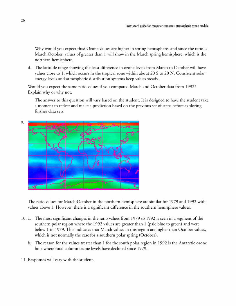
The ratio values for March:October in the northern hemisphere are similar for 1979 and 1992 withvalues above 1. However, there is a significant difference in the southern hemisphere values.

10. a. The most significant changes in the ratio values from 1979 to 1992 is seen in a segment of thesouthern polar region where the 1992 values are greater than 1 (pale blue to green) and werebelow 1 in 1979. This indicates that March values in this region are higher than October values,which is not normally the case for a southern polar spring (October).

b. The reason for the values treater than 1 for the south polar region in 1992 is the Antarctic ozonehole where total column ozone levels have declined since 1979.

11. Responses will vary with the student.

27


exercise 7using monthly and annual averages to

monitor seasonal changes and change intotal global ozone for 1979 and 1992

In Exercise 4 students used monthly images ofTOMS ozone values to observe the seasonal fluc-tuations of atmospheric ozone levels for 1979. Inthis exercise they observe seasonal changes in themonthly average images for 1992 and comparethese values to 1979 images to note changes thatmay have occurred over time.


Visually analyze temporal trends in ozone lev-els from images in a montage and an ani-mation.

Generate a yearly average image for compari-son with monthly average images.




science process skillsobservingmeasuringinferringcommunicatingpredictinginterpreting data

image processing skillsimporting multiple imagesapplying a color tableapplying an overlay imagegenerating an image stackcalculating the average image of an image

stack using a macromaking a montage from an image stackanimating an image stack

mathematical tools and skillsaveraging image data using a prewritten macro


Morphology of Ozone

28



1. Ozone values are higher over a larger region of the north polar regions during its spring. Valuesgenerally decrease in the southern polar region for its spring.

2. a. Ozone seems to be distributed along lines of latitude more than longitudinally.

b. Meridionally. Zonal winds allow mixing within a latitude band on a relatively short time scale.Meridional mixing (i.e., Brewer Dobson circulation) involves larger scale circulation dynamicsand takes longer.

3. a. Maximum 463 (#3) Minimum 147 (#10)Color bright yellow color purple

Greatest changes in ozone values occur in the north and south polar regions. Changes are basedon atmospheric transport processes and differential production rates caused by varied solarinsolation at the poles.

b. Greatest changes in polar regions with highs occurring in northern hemisphere spring and lowsin southern hemisphere spring; tropical and mid-latitudes ozone values do not vary as widelywith seasons.

29


4. There is a visible decrease in the ozone values in the northern hemisphere for the first four months of1992 compared to 1979.

5. Looking at all the months on both montages for the tropical regions there has been a decline in theozone values.

6. Both the north polar and south polar regions have values that vary as much as 100 DU with 1992values being less than 1979. Ozone values in the south polar region hit lows near 150 DU. Thesouth polar region has experienced a large change in values from September through December.

7. Answers will vary. Each pixel on the average should have values closer to the mean so the image willhave less color variation.

8. a. There is less variation at any latitude on the yearly average image than on any of the monthlyaverage images. The difference between north and south polar distributions is still evident.

b. This answer will depend on what a student predicted previously.

c. Values range from 235 to 381 DU with higher values in south mid-latitudes, north mid-lati-tudes, and north polar regions. Lowest values occur in the south polar region. The southernhemisphere polar values are 50–100 DU lower than comparable values in the northern hemi-sphere polar regions.

30


31


exercise 8investigating ozone distributions in 1979

and 1992 using monthly and yearlyglobal ozone values

This activity is an extension of Exercise 7 that in-vestigates changes in ozone value from 1979 to1992. Students generate and analyze standard de-viation images from monthly average images andcompute means for monthly and yearly averageozone distributions to investigate temporal chang-es.


Generate and interpret a standard deviationimage from monthly average images ofozone distribution.

Compute global monthly and yearly meanozone values from monthly average images.

Analyze temporal trends in ozone levelsthrough mean and standard deviation imag-es.




science process skillsobservingmeasuringinferringcommunicatingpredictinginterpreting data

image processing skillsimporting multiple imagesapplying a color tablegenerating an image stackcalculating the average image of an image

stack using a macrocalculating the standard deviation image of an

image stack using a macrocalculating a ratio image from two images us-

ing image mathematics

mathematical tools and skillsaveraging image data using a prewritten macrogenerating and interpreting a standard devia-

tion imageinterpreting ratios


Morphology of Ozone

32



1. a. color for least SDpurple

b. color for greatest SDred

2. a. Tropical region shows leaststandard deviation in ozonevalues. Tropical ozone distribu-tions do not generally exhibitseasonal changes.

b. Greatest change is seen in thenorth polar region where thereare significant seasonal changescaused by varied amounts ofinsolation and atmosphericdynamics.

image mean standarddeviation (sd)

# month 1979 1992 1979 1992

1 January 293 284 47 43

2 February 296 288 55 43

3 March 301 290 55 45

4 April 304 292 50 44

5 May 303 292 44 39

6 June 301 289 37 37

7 July 300 289 32 31

8 August 302 289 31 30

9 September 304 289 35 30

10 October 301 286 47 32

11 November 296 282 42 31

12 December 293 277 40 30

13Yearly Avg.

Ozone300 287 37 31

33


3. a. The seasonal cycle in ozone shows lowest values in the northern hemisphere winter months. Theseasonal cycle is a complex combination of ozone transport, production, and destruction cyclesthat differ in magnitude in the northern and southern hemispheres. See Chapter 8 on OzoneVariability for a detailed discussion of the factors affecting this cycle.

b. Month(s) varying the most: February–April and October; these are spring and fall months whenchanges in dynamics and insolation will affect ozone levels more.

c. In general, you should note that the spring and autumn values standard deviation values aregreater than comparable values for summer and winter months. Have students graph the stan-dard deviation values as a function of month to see the pattern.

4. a. Months varying the most: DecemberSee answer to 3

b. Months varying the least: February and OctoberAugust and December might be expected since they are summer and winter monthsSee answer to 3

5. a. All monthly mean values are lower in 1992 than in 1979.

b. The average yearly value in 1992 is 4% lower than the comparable value for 1979.

c. The same trend can be seen in both sets of values except for the period from June to Septemberand December. For 1979 and 1992, February, March, April deviate more. October stands out inthe standard deviation in 1979 but not in 1992.

d. There is greater variation in the standard deviation values for 1979, showing seasonal differences.There is less variation in 1992 notable in the period from August to December indicating thatsome process(es) that influences southern hemisphere spring values is different in 1992 than in1979.

34


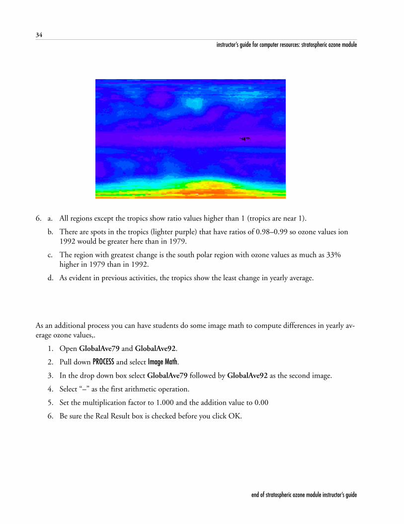
6. a. All regions except the tropics show ratio values higher than 1 (tropics are near 1).

b. There are spots in the tropics (lighter purple) that have ratios of 0.98–0.99 so ozone values ion1992 would be greater here than in 1979.

c. The region with greatest change is the south polar region with ozone values as much as 33%higher in 1979 than in 1992.

d. As evident in previous activities, the tropics show the least change in yearly average.

As an additional process you can have students do some image math to compute differences in yearly av-erage ozone values,.

1. Open GlobalAve79 and GlobalAve92.

2. Pull down PROCESS and select Image Math.

3. In the drop down box select GlobalAve79 followed by GlobalAve92 as the second image.

4. Select “–” as the first arithmetic operation.

5. Set the multiplication factor to 1.000 and the addition value to 0.00

6. Be sure the Real Result box is checked before you click OK.

end of stratospheric ozone module instructor’s guide

stratospheric ozone module - ccpo · 1978–1992 to satellite operations or envi- ... stratospheric...

Documents