strategies for setting futility analyses at multiple time points in clinical trials
TRANSCRIPT

at multiple time points in clinical trials
Lu Mao, PhD Student
University of North Carolina at Chapel Hill
Supervisor: Paul Gallo, PhD
Strategies for Futility Analyses

OUTLINE
| Lu Mao | 08/14/2012 | Futility analyses | Business Use Only 2
Background for Futility Analysis
• Motivation
• B-value theory
• Conditional Power
• Predictive Power
Methods and Results
• Two futility looks
• Three futility looks
Software (R) Demonstration
Conclusion
Stop for Futility
BACKGROUND - MOTIVATION
| Lu Mao | 08/14/2012 | Futility analyses | Business Use Only 3
Traditional Design: fix the sample size and perform analyses after all subjects have been recruited.
Group Sequential Design: several interim analyses are conducted in the course of patient enrollment
• Safety
• Early determination of (in)efficacy
• Ethics
• Cost reduction
Futility Analysis: a group sequential design to allow for early termination of the trial when the likelihood of establishing efficacy at final stage is decide to be low.

BACKGROUND - MOTIVATION
An ideal futility analysis design:
1. Considerably curtails the length of the trial when there is no/negative effect
2. Do not substantially affect the operating characteristics (Type I and Type II errors) of the original fixed-sample design.
| Lu Mao | 08/14/2012 | Futility analyses | Business Use Only 4
H0
HA
Futility rules
Final
Analysis
STOP

BACKGROUND - STATISTICAL TOOLS
| Lu Mao | 08/14/2012 | Futility analyses | Business Use Only 5
Group sequential trials – multiple testing on several statistics based on the first m observations, m=n1,...,nk
Let the test statistics, e.g. z scores, be . The rejection region R={|Zn|>z1-α/2}
If Z>0 means a positive effect for the treatment, we wish to stop the trial for futility when the interim Z scores are very low, e.g. set (zn1
,...,znk), and at the i’th interim,
Needs to find the joint distribution of
),,...,(1 nnn ZZZ
k
),,...,(1 nnn ZZZ
k
ii nn zZ Stop to
Accept H0

BACKGROUND - STATISTICAL TOOLS
Typically, the Z statistic calculated from the first m obs can be expressed in terms of a partial sum statistic in the form
where is an estimate of , the variance of .
Example: Two sample normal test
| Lu Mao | 08/14/2012 | Futility analyses | Business Use Only 6
m
i imS1
m
SZ m
m
0
1
0ˆ2
)(
ˆ2
)(
m
YXYXm
Z
m
i
ii
m
2 i2

BACKGROUND - B-VALUE THEORY
Easier to find the joint distribution of by the well known Brownian motion approximation to the partial sums.
Indeed, if is the effect size (true state of nature),
where is related to the true state of nature and the overall sample size, and is the fraction of sample size at the j’th interim, call it information time. Obviously
| Lu Mao | 08/14/2012 | Futility analyses | Business Use Only 7
),,...,(1 nnn SSS
k
1
,
1
11
1
1
1111
1
1
1
1
1
k
kkk
d
n
i i
n
i i
n
i i
n
n
n
tt
ttt
ttt
t
t
Nn
S
S
S
nk
k
iE
n
kjnnt jj ,,1, .10 jt

BACKGROUND - B-VALUE THEORY
Call the left side of the previous formula the B values, denoted .
We have seen that the B scores follow the marginal distribution of a standard Brownian motion with drift term θ
The relationship between the Z scores and the B scores is simple:
Or:
| Lu Mao | 08/14/2012 | Futility analyses | Business Use Only 8
))1(),(,),(( 1 BtBtB k
)(1
ˆˆj
j
n
jj
n
n tBtn
S
n
n
n
SZ
jj
j
jnjj ZttB )(

BACKGROUND - CONDITIONAL POWER
Conditional Power: quantifies the notion of likelihood of success given the current data
Futility rule: stop at the j’th interim if
Since , we have
Therefore
| Lu Mao | 08/14/2012 | Futility analyses | Business Use Only 9
kjbtBzBPbCP jjj ,,1),;)(|)1(();( 2/1
.));(( jjtBCP
1,
1)1(
)(
j
jjjj
t
tttN
B
tB
jjjj tttBNtBB 1,)1()(,)()1(
j
jj
jt
btzbCP
1
)1(1);(
2/1

BACKGROUND - CONDITIONAL POWER
Conditional power based on the hypothesized 𝜃 does not allow the state of nature to adapt to the observed data.
Conditional power based on the current estimate 𝜃 𝑗
𝐶𝑃 𝑏𝑗; 𝜃 𝑗 ≡ 𝑃 𝐵 1 > 𝑧1−
𝛼2
𝐵 𝑡𝑗 = 𝑏𝑗; 𝜃 𝑗
Recall that 𝐵 𝑡𝑗 ∼ 𝑁 𝑡𝑗𝜃, 𝑡𝑗 , we obtain
𝜃 𝑗 = 𝐵(𝑡𝑗)/𝑡𝑗
𝐶𝑃 𝑏𝑗; 𝜃 𝑗 = 1 − Φ𝑧1−𝛼 2 −𝜃 𝑗 1−𝑡𝑗 −𝑏𝑗
1−𝑡𝑗= 1 − Φ
𝑧1−𝛼 2 −𝑏𝑗 𝑡𝑗
1−𝑡𝑗
| Lu Mao | 08/14/2012 | Futility analyses | Business Use Only 10

BACKGROUND - PREDICTIVE POWER
Another way of allowing the state of nature to adapt to the observed data is (Bayesian) predictive power.
Predictive power – conditional power averaged over the posterior distribution of the state of nature:
𝑃𝑃 𝑏𝑗; 𝜋 ⋅ = ∫ 𝐶𝑃 𝑏𝑗; 𝜃 𝜋 𝜃 𝑏𝑗 𝑑𝜃
Typically, we take the uniform prior: 𝜋 𝜃 ∝ 1
After some derivation, we obtain
𝑃𝑃 𝑏𝑗; 𝜋 ⋅ ≡ 1 = 1 − Φ𝑡𝑗𝑧1−𝛼 2 − 𝑏𝑗 𝑡𝑗
1 − 𝑡𝑗
| Lu Mao | 08/14/2012 | Futility analyses | Business Use Only 11

BACKGROUND - POWER FUNCTION
We have seen three ways of choosing the futility boundary (𝑏1, ⋯ , 𝑏𝑘)
1. Conditional power: 𝐶𝑃
2. Conditional power based on current estimate: 𝐶𝑃(𝜃 )
3. Predictive power: 𝑃𝑃
Given the boundary, the power function is given by
Ψ 𝜃 ≡ 𝑃 Reject 𝐻0 𝜃 = P𝜃 B tj ≥ 𝑏𝑗 , 𝑗 = 1, ⋯ , 𝑘, B 1 > z1−𝛼 2
< 𝑃𝜃 𝐵(1) > z1−𝛼 2
| Lu Mao | 08/14/2012 | Futility analyses | Business Use Only 12

BACKGROUND - ERROR PROBABILITIES
Thus the power function is reduced when either 𝜃 = 0 or equals hypothesized effect size
In statistical language, both the type I error rate and power are decreased.
Power loss: a fraction of successful trials are terminated by the futility rule.
| Lu Mao | 08/14/2012 | Futility analyses | Business Use Only 13

BACKGROUND - PREVIOUS STUDIES
Chang et al. 2004
• Assesses one futility look at midway of trial based on conditional power;
• Shows that most power loss can be “reclaimed” by lowering the (final) critical value to achieve type I error rate exactly 𝛼;
(recall that for critical value 𝑧1−𝛼 2 the overall type I error < 𝛼)
• Provides a graphical method of doing this
Lachin et al. 2005
• One futility look based on conditional power at midway
• Suggests an iterative algorithm of determining the critical value that achieves 𝛼 to regain power.
| Lu Mao | 08/14/2012 | Futility analyses | Business Use Only 14

BACKGROUND - PREVIOUS STUDIES
Snapinn et al. 2006
• Reviews conditional power approach to futility rule;
• Note the problem of reclaiming 𝛼: rules become binding, while it crosses the boundary it has to stop.
Emerson et al. 2005
• Considers CP, CP(𝜃 ), PP and various other scales in determining futility rules
• Argues that the scale used is less important than the resulted operating characteristics.
V. Shih & P. Gallo 2010
• Investigate power loss vs sample size reduction for one futility rule
at midway based on CP, CP(𝜃 ), PP.
| Lu Mao | 08/14/2012 | Futility analyses | Business Use Only 15

METHODS – GENERAL
Rationale
• Nonbinding futility rule: no type I error reclaiming;
• ASN (average sample number) under 𝐻0 is the optimization target, provided that other factors are controlled;
• To regain power, we may enlarge the sample size – sample size inflation (SI) is the control target;
• No power regaining – power loss is the control target.
Setting
• Multiple futility looks at arbitrary time points – For simplicity and practicality we only consider two and three looks at evenly spaced interims;
• Different scales (CP, CP(𝜃 ), PP, etc ) of setting futility rules.
| Lu Mao | 08/14/2012 | Futility analyses | Business Use Only 16

METHODS – GENERAL
Aim
• Setting up a theoretical framework for nonbinding futility rules;
• Comparing numerical results using different scales CP, CP(𝜃 ) and PP;
• Develop easy-to-implement program, based on efficient numerical algorithms, to allow the user to choose different scales, values of the scale, and setup of interim time points.
Facilities
• Most numerical analyses are done in R; a few in MatLab;
• We make use of the R package mvtnorm for multivariate normal distribution function evaluations.
| Lu Mao | 08/14/2012 | Futility analyses | Business Use Only 17
METHODS – SAMPLE SIZE INFLATION
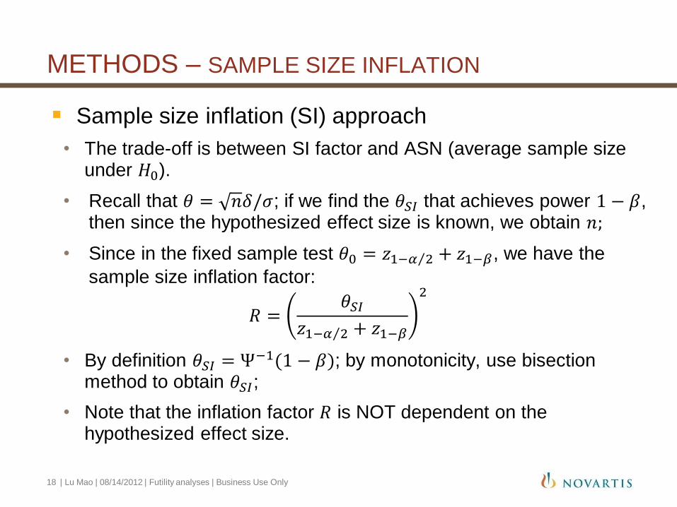
Sample size inflation (SI) approach
• The trade-off is between SI factor and ASN (average sample size under 𝐻0).
• Recall that 𝜃 = 𝑛𝛿/𝜎; if we find the 𝜃𝑆𝐼 that achieves power 1 − 𝛽, then since the hypothesized effect size is known, we obtain 𝑛;
• Since in the fixed sample test 𝜃0 = 𝑧1−𝛼 2 + 𝑧1−𝛽, we have the
sample size inflation factor:
𝑅 =𝜃𝑆𝐼
𝑧1−𝛼 2 + 𝑧1−𝛽
2
• By definition 𝜃𝑆𝐼 = Ψ−1(1 − 𝛽); by monotonicity, use bisection method to obtain 𝜃𝑆𝐼;
• Note that the inflation factor 𝑅 is NOT dependent on the hypothesized effect size.
| Lu Mao | 08/14/2012 | Futility analyses | Business Use Only 18

METHODS – POWER LOSS
Power loss approach:
• Without SI to regain power;
• We look at equal
- CP
- CP(𝜃 )
- PP
- Equal power loss (Power loss at tj: 𝑙𝑗 𝜃 = 𝑃𝜃(𝐵 𝑡𝑖 ≥ 𝑏𝑖 , 𝑖 = 1 ⋯ , 𝑗 −
1, 𝐵 𝑡𝑗 < 𝑏𝑗 , 𝐵 1 > 𝑧1−𝛼 2 ))
at two and three evenly spaced interims.
• The trade-off is between power loss and ASN
• We also assess the optimal rules (the rules that result in minimum ASN given certain power loss)
- Optimization done by grid search
| Lu Mao | 08/14/2012 | Futility analyses | Business Use Only 19

RESULTS – SAMPLE SIZE INFLATION
| Lu Mao | 08/14/2012 | Futility analyses | Business Use Only 20
SI factor
• To achieve 1 − 𝛽 = 0.9 based on equal conditional power 𝛾 at 𝑘 = 1, ⋯ , 5 evenly spaced interims
• when 𝛾 ≤ 0.5, inflation is in fact negligible (≤ 1.1), indicating great practicality in applying these non-binding futility rules through SI.
SI Conditional power 𝛾
k 0.2 0.3 0.4 0.5 0.6 0.7 0.8
1 1.002 1.007 1.018 1.038 1.073 1.129 1.221
2 1.006 1.016 1.033 1.063 1.106 1.175 1.282
3 1.009 1.022 1.045 1.078 1.130 1.201 1.314
4 1.011 1.029 1.054 1.092 1.145 1.222 1.337
5 1.015 1.033 1.061 1.102 1.159 1.237 1.355

RESULTS – SAMPLE SIZE INFLATION
ASN
• Same setting as the previous table
• There is substantial reduction of sample size for k=2, 3, 𝛾 ≤ 0.5 , a practical range of futility looks with tolerable SI.
| Lu Mao | 08/14/2012 | Futility analyses | Business Use Only 21
ASN Conditional power 𝛾
k 0.2 0.3 0.4 0.5 0.6 0.7 0.8
1 0.823 0.766 0.722 0.691 0.675 0.674 0.696
2 0.756 0.715 0.678 0.647 0.622 0.609 0.609
3 0.716 0.677 0.648 0.622 0.604 0.588 0.582
4 0.693 0.657 0.628 0.606 0.589 0.578 0.571
5 0.680 0.643 0.615 0.595 0.580 0.569 0.563

RESULTS – SAMPLE SIZE INFLATION
| Lu Mao | 08/14/2012 | Futility analyses | Business Use Only 22
Additional issue with SI
• Power=1 − 𝛽 at hypothesized effect size, by construction;
• Need to assess the global power behavior, especially those near the hypothesized 𝛿
• The right figure shows that the power curves for the “SI”ed futility design are almost indistinguishable from those of the fixed sample (reference) design when 𝛿 ≥ 0.5 ∗ (designed 𝛿)

RESULTS – POWER LOSS
Two futility looks
| Lu Mao | 08/14/2012 | Futility analyses | Business Use Only 23
Power loss Equal CP
Equal
CP(𝜃 ) Equal PP Equal
power loss Optimal
0.002 0.751 0.769 0.724 0.722 0.717
0.003 0.726 0.727 0.696 0.692 0.689
0.005 0.700 0.692 0.663 0.665 0.661
0.007 0.674 0.658 0.636 0.640 0.635
0.010 0.648 0.627 0.611 0.615 0.610
0.015 0.620 0.596 0.584 0.591 0.584
0.021 0.591 0.565 0.557 0.567 0.557
0.029 0.562 0.537 0.532 0.544 0.532
0.041 0.532 0.508 0.506 0.520 0.505

RESULTS – POWER LOSS
Equal PP is the closest to the optimal bound over all;
Equal power loss approximates the optimal bound only when power loss is very small.
| Lu Mao | 08/14/2012 | Futility analyses | Business Use Only 24

RESULTS – POWER LOSS
Three futility looks
| Lu Mao | 08/14/2012 | Futility analyses | Business Use Only 25
Power loss Equal CP
Equal
CP(𝜃 ) Equal PP Equal
power loss Optimal
0.003 0.708 0.738 0.680 0.673 0.661
0.005 0.683 0.708 0.644 0.641 0.631
0.007 0.659 0.678 0.618 0.620 0.611
0.010 0.635 0.637 0.593 0.594 0.584
0.014 0.610 0.600 0.563 0.569 0.559
0.020 0.584 0.564 0.536 0.548 0.534
0.028 0.556 0.528 0.508 0.522 0.507
0.037 0.527 0.495 0.482 0.500 0.481
0.051 0.495 0.462 0.454 0.476 0.453

RESULTS – POWER LOSS
Overall, equal PP performs best of all, again; less satisfactory for small power loss;
Similarly, equal power loss is doing well for small power losses but not so for greater ones.
| Lu Mao | 08/14/2012 | Futility analyses | Business Use Only 26

RESULTS – OPTIMAL BOUNDS
Optimal bounds for two futility looks (precision 0.001)
| Lu Mao | 08/14/2012 | Futility analyses | Business Use Only 27
Power
loss
𝑧1(𝛾1) 𝑧2(𝛾2)
𝑧3 ASN
0.002 -0.852 (0.361) 0.371 (0.159) 1.960 0.717
0.003 -0.674 (0.409) 0.449 (0.187) 1.960 0.689
0.005 -0.518 (0.452) 0.527 (0.218) 1.960 0.661
0.007 -0.383 (0.490) 0.615 (0.257) 1.960 0.635
0.010 -0.259 (0.525) 0.693 (0.294) 1.960 0.610
0.015 -0.103 (0.569) 0.732 (0.313) 1.960 0.584
0.021 0.032 (0.606) 0.815 (0.355) 1.960 0.557
0.029 0.170 (0.643) 0.884 (0.392) 1.960 0.532
0.041 0.314 (0.680) 0.966 (0.437) 1.960 0.505

RESULTS – OPTIMAL BOUNDS
Optimal bounds for three futility looks (precision 0.01)
| Lu Mao | 08/14/2012 | Futility analyses | Business Use Only 28
Power
loss
𝑧1(𝛾1) 𝑧2(𝛾2)
𝑧3(𝛾3)
𝑧4 ASN
0.003 -1.13(0.457) -0.09(0.284) 0.63(0.112) 1.96 0.661
0.005 -0.98(0.491) 0.00(0.316) 0.79(0.174) 1.96 0.631
0.007 -0.86(0.519) 0.08(0.345) 0.84(0.201) 1.96 0.611
0.010 -0.66(0.565) 0.16(0.375) 0.86(0.209) 1.96 0.584
0.014 -0.49(0.603) 0.21(0.394) 0.90(0.229) 1.96 0.559
0.020 -0.38(0.627) 0.34(0.444) 0.94(0.250) 1.96 0.534
0.028 -0.22(0.662) 0.43(0.480) 0.94(0.251) 1.96 0.507
0.037 -0.08(0.691) 0.48(0.500) 1.05(0.312) 1.96 0.481
0.051 0.02(0.711) 0.67(0.575) 1.10(0.346) 1.96 0.453

RESULTS – DISCUSSION
Equal conditional power is not a good idea for futility rule at multiple time points;
Intuitively, the conditional power does not adapt to the observed data as it moves along;
The same conditional at a later point means drastically different things comparing to an earlier point, if the early data are already contradicting the hypothesized 𝜃.
Allowing the state of nature to adapt is probably the reason for the success of equal PP.
Note that our findings SHOULD NOT be taken to mean that the idea of conditional power is bad.
| Lu Mao | 08/14/2012 | Futility analyses | Business Use Only 29

RESULTS – DISCUSSION
Compare the bounds:
• This is the futility bounds for power loss 0.01;
• Equal PP and optimal bounds coincide very well;
• Comparing to the optimal, equal CP is conservative in the beginning and aggressive in the end;
equal CP(𝜃 ) is aggressive in the beginning and conservative in the end.
| Lu Mao | 08/14/2012 | Futility analyses | Business Use Only 30
DEMONSTRATION OF fut()
| Lu Mao | 08/14/2012 | Futility analyses | Business Use Only 31
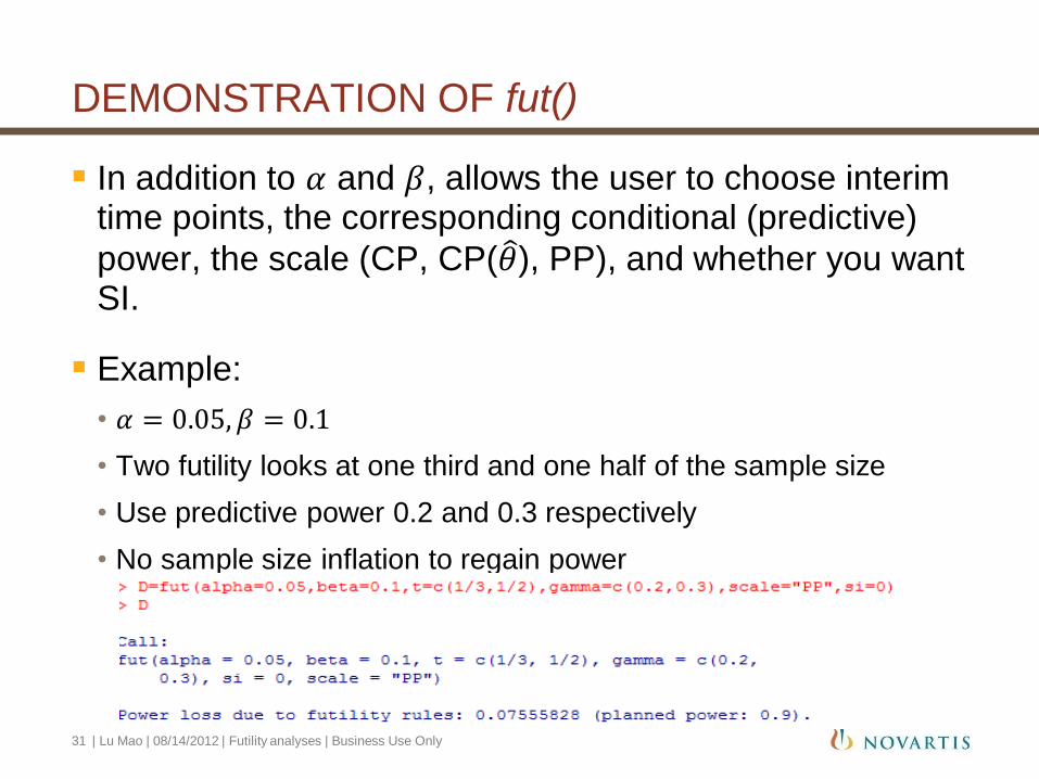
In addition to 𝛼 and 𝛽, allows the user to choose interim time points, the corresponding conditional (predictive)
power, the scale (CP, CP(𝜃 ), PP), and whether you want SI.
Example:
• 𝛼 = 0.05, 𝛽 = 0.1
• Two futility looks at one third and one half of the sample size
• Use predictive power 0.2 and 0.3 respectively
• No sample size inflation to regain power

DEMONSTRATION OF fut()
• Use the summary() function to print out the details:
| Lu Mao | 08/14/2012 | Futility analyses | Business Use Only 32

DEMONSTRATION OF fut()
• Plot the boundary: >plot(D)
| Lu Mao | 08/14/2012 | Futility analyses | Business Use Only 33
• Plot the power function >powerplot(D)

CONCLUSIONS
We have established an SI framework to non-binding futility rule with uncompromised power;
We have shown that in realistic situations (𝑘 = 2, 3), equal PP across the time points results in approximately optimal (in terms of ASN) bounds.
We have developed an easy-to-use R program fut() for design of nonbinding futility rules.
| Lu Mao | 08/14/2012 | Futility analyses | Business Use Only 34

THANK YOU FOR YOUR ATTENTION!
QUESTIONS
| Lu Mao | 08/14/2012 | Futility analyses | Business Use Only 35