Strategies for project scheduling with alternative subgraphs underuncertainty: similar and dissimilar sets of schedules

Tom Servranckxa, Mario Vanhouckea,b,c,∗

aFaculty of Economics and Business Administration, Ghent University, Tweekerkenstraat 2, 9000 Ghent(Belgium)

bOperations and Technology Management Centre, Vlerick Business School, Reep 1, 9000 Ghent (Belgium)cUCL School of Management, University College London, 1 Canada Square, London E14 5AA (UK)

Abstract

In the resource-constrained project scheduling problem with alternative subgraphs (RCPSP-

AS), we model alternative execution modes for work packages in the project. In contrast

to the traditional RCPSP, the project network consists of different alternative work pack-

ages. To that purpose, the scheduling problem selects the best possible alternatives for

the construction of the baseline schedule. On top of that, several back-up schedules are

created in order to cope with unexpected changes along the project progress. In the pres-

ence of uncertainty, we can then switch between these alternative schedules at different

decision moments in order to bring the project back on track. The alternative schedules

are combined in a set of schedules that should be constructed by the project manager prior

to project execution. We present a computational experiment to investigate the ability of

using such a set of schedules in the presence of uncertainty during project execution. The

experiments indicate that using a set of schedules outperforms the use of a single schedule,

even when the uncertainty level is relatively low. The results also show that the composi-

tion of this schedule set is important. Therefore, a degree of schedule similarity is proposed

to analyse this composition, and results show that a mix of similar and dissimilar schedules

performs best. Finally, we show that the solution quality of each schedule in the set has

an impact on the performance of the schedule switches given the project disruptions.

Keywords: Project scheduling, Alternative subgraphs, Simulation, Scenario analysis

∗Corresponding authorEmail addresses: tom.servranckx@ugent.be (Tom Servranckx), mario.vanhoucke@ugent.be (Mario

Vanhoucke)

Preprint submitted to Elsevier February 25, 2021

0.1. Introduction

Most research efforts in the resource-constrained project scheduling problem (RCPSP)

have focused on the development of (meta)heuristic and optimal solution procedures to

obtain (sub)optimal project schedules subject to various constraints (Weglarz et al., 2011).

In deterministic project scheduling problems, it is assumed that all information about the

project (i.e. activity durations, resource requirements and availabilities, etc.) is static and

known in advance. However, this assumption is rendered obsolete in most practical situ-

ations as projects should be scheduled in an uncertain and highly complex environment

(Vidal et al., 2011; Marle and Vidal, 2016). As a result, the frequency and impact of dis-

ruptions during project execution is expected to increase. The problem is that, from the

moment a disruption occurs, the solution quality of the baseline project schedule deterio-

rates as it becomes impossible or impractical to implement in the new project environment.

In the face of uncertainty, several approaches have been proposed in literature to cope

with the disruptions between the baseline and the actual project schedule. The most

common approaches for project scheduling under uncertainty are proactive and reactive

scheduling approaches (Herroelen and Leus, 2005). Most recent research efforts focus on

improving the robustness of a single project schedule in order to deal with disruptions in

the project environment. Moreover, the robust scheduling approaches can only alter the

start times of the activities in order to improve the robustness of the baseline schedule,

which still limits the flexibility during scheduling under uncertainty. However, Herroelen

and Leus (2005) further indicate that the robustness of project scheduling can be increased

by generating multiple baseline schedules, rather than a single one, before project execu-

tion. This approach, called contingent scheduling, increases the flexibility in the project

scheduling phase as it allows the decision maker to switch between schedules in order to

respond to unexpected events. Consequently, it combines beneficial properties of both

proactive and reactive scheduling techniques. Moreover, Esswein and Billaut (2002) in-

dicate that there exists a trade-off between the solution quality and the robustness of a

schedule. More precisely, the quality of a schedule obtained using a proactive strategy will

deteriorate since it should be robust for a wide variety of disruption scenarios. In contrast,

we can generate a set of higher-quality schedules with a lower individual robustness, while

a higher overall robustness of the set of schedules is maintained.

Servranckx and Vanhoucke (2019) have introduced the resource-constrained project

scheduling problem with alternative subgraphs (RCPSP-AS), which extends the RCPSP

by relaxing the assumption of a fixed project structure and assuming alternative ways to

2

execute work packages of the project. One alternative execution mode should be selected

for each work package (i.e. the selection subproblem) and, subsequently, the corresponding

activities should be scheduled (i.e. the scheduling subproblem) such that the makespan

of the project is minimised. However, the authors study this problem in the absence of

uncertainty. Consequently, this research aims to combine two promising research avenues

on scheduling under uncertainty. On the one hand, the existing research on the generation

of multiple schedules does not consider that the project structure underlying these schedules

might differ. On the other hand, the improved flexibility in the project structure of the

RCPSP-AS is not used to cope with uncertainty. In summary, we construct multiple

baseline schedules incorporating the alternative subgraphs to protect the actual project

makespan against uncertainty.

Due to the existence of alternative execution modes of work packages in the RCPSP-AS,

we can adjust both the start times of the selected activities (i.e. scheduling subproblem)

and the selection of alternative execution modes for the work packages (i.e. selection

subproblem) in order to construct multiple baseline schedules. In other words, the proposed

problem formulation allows the construction of alternative schedules, which might differ

with respect to the selected alternatives, and the combination of these alternative schedules

in a set of schedules. Consequently, the existence of alternative subgraphs can be exploited

to respond to uncertain events by switching between different alternative schedules in

the set of schedules. This results in several back-up schedules in case that the baseline

schedule becomes inferior due to disruptions. In contrast to the existing research efforts

on contingent scheduling, these back-up schedules might be supported by distinct project

structures as they represent alternative ways to execute the project. In the presence of

uncertainty, the ability to change alternatives is considered a crucial option to manage

highly complex projects. In case of an uncertain event, a back-up schedule can be selected

that consists of completely different selected alternatives and thus presents a completely

different approach to the project. In this research, we further develop different strategies

to construct the set of schedules. The performance of these strategies is evaluated based

on the ability to protect the project makespan against various types of uncertainty.

In summary, the contributions of this research are fourfold. (1) To the best of our

knowledge, this is the first research effort to investigate the overall impact of different types

and degrees of uncertainty (i.e. duration variability, resource unavailability and resource

inefficiencies) on the project scheduling problem with alternative subgraphs. (2) Moreover,

we present a scheduling approach under uncertainty for the proposed problem formulation.

3

(3) Also, some managerial insights are provided on the performance of different strategies

to construct the set of schedules in various practical settings. (4) Finally, this paper allows

quantifying the impact of the characteristics of alternative subgraphs on the ability to cope

with the disruptions through the different strategies.

The outline of this paper is organised as follows. Section 3.2 provides a brief overview

of the literature on project scheduling under uncertainty. In section 3.3, the resource-

constrained project scheduling problem with alternative subgraphs is briefly explained.

In section 3.4, the different steps of the solution approach are explained and illustrated

using an example project. The experimental design and the computational results of the

simulation experiments are discussed in section 3.5. Finally, section 3.6 provides some

general conclusions and suggestions for future research.

0.2. Literature overview

In this section, we will discuss the main literature on three project scheduling techniques

to deal with uncertainty: proactive, reactive and contingent scheduling.

Proactive (robust) project schedules anticipate future disruptions using statistical knowl-

edge of uncertainty and absorb these disruptions without the need to reschedule (Herroelen

and Leus, 2005). More precisely, the objective in proactive scheduling is to generate a base-

line schedule that is stable over a set of disturbance scenarios. Herroelen and Leus (2004)

provide an overview and a detailed description of variants of the robust project scheduling

problem. Van de Vonder et al. (2005) develop several (meta)heuristics to generate robust

predictive schedules. An important aspect of proactive project scheduling is the difference

between two definitions of robustness. Quality robustness refers to the stability of the

objective value of a solution when disruptions occur. Jensen (2001) defines the stability

of quality robust schedules by means of the worst-case performance and worst deviation

performance. Solution robustness ensures that the activity start times of the baseline

schedule are stable under a wide range of project execution scenarios. The stability of

solution robust schedules can be measured by the expected weighted deviations in start

times between the realised and baseline schedule (Herroelen and Leus, 2004) or by the

weighted number of late jobs (Sevaux and Sorensen, 2004). We can also identify several

techniques to generate robust schedules in literature. Goa (1995) generates robust sched-

ules by augmenting the duration of activities that require breakable resources, which are

resources with a non-zero probability of breakdown, and by applying baseline scheduling

techniques. Davenport et al. (2001) do not extend the duration of individual activities,

4

but rather explicitly include slack time per activity in the schedule. Tavares et al. (1998)

introduce the concept of a float factor to obtain schedules that are positioned between

the earliest and latest start schedule. This is important since an optimal trade-off should

be established between the high discounted cost of the project in case of an earliest start

schedule and the high risk of delays in case of a latest start schedule.

In case of major disruptions, it might be necessary to repair the baseline project schedule

using reactive scheduling (Herroelen and Leus, 2005). Such scheduling techniques deal with

the revision or re-optimisation of the baseline schedule after unexpected events occur rather

than the preparation of the baseline schedule for the uncertainty. We refer to Van de Vonder

et al. (2007) for a discussion of reactive strategies and several heuristic solution approaches

for reactive scheduling under multiple activity duration disruptions. The main difference

between proactive and reactive strategies is the frequency of decision making. In proactive

strategies, a single scheduling decision is made prior to project execution, while reactive

strategies correspond to a multi-stage decision-making process during project execution.

This high number of decisions in reactive scheduling is a disadvantage since stable project

schedules are important for in-house resource management and subcontractor agreements

(Wiers, 1997). Consequently, proactive-reactive scheduling techniques have been developed

in order to combine the stability of robust strategies and the responsiveness of reactive

strategies. Van de Vonder et al. (2006) show that proactive-reactive strategies result in

stable project schedules with a high makespan performance.

So far, two distinct strategies have been discussed to construct a single project schedule

under uncertainty. Another approach is to generate multiple schedules prior to project ex-

ecution, so-called contingent scheduling (Herroelen and Leus, 2005), such that the decision

maker can shift from one schedule to another in case that the project environment changes.

In the field of job shop scheduling, Billaut and Roubellat (1996b) generate a set of schedules

that is specified in terms of the sequence of operations on the resources. More precisely, a

group sequence is generated for each resource as a partially or totally ordered set of groups

of operations. The set of schedules is constructed by arbitrarily ordering the operations

inside each group. The concept of a group sequence is subsequently applied in the context

of single machine scheduling (Aloulou et al., 2002; Mauguire et al., 2002; Briand et al.,

2007), multiple renewable resources (Billaut and Roubellat, 1996a), multi-mode scheduling

with minimal and maximal time-lags (Briand et al., 2002) and multi-mode project schedul-

ing problems with a release and a due date (Artigues et al., 1999). Furthermore, Artigues

et al. (2005) present a representation of such a family of schedules based on the ordered

5

group assignment problem in general shop scheduling (Wu et al., 1999). Also, Artigues

et al. (2005) are first to provide a worst-case evaluation of the set of schedules with respect

to the scheduling objective and the authors provide two objective values to measure the

degree of flexibility in the set of schedules with the aim of maximising the robustness of the

proposed set of schedules. They consider the generation of a set of schedules that balances

the maximisation of the obtained flexibility, and hence the robustness of the proactive

scheduling approach, and the maximisation of the scheduling objective.

Based on the above literature overview, we can conclude that proactive-reactive strate-

gies are an important future avenue in project scheduling under uncertainty. Our proposed

solution approach combines elements from both proactive and reactive strategies. More-

over, our approach is closely related to contingent scheduling since we will generate multiple

alternative schedules to cope with project disruptions. The literature shows that contingent

scheduling has been successfully implemented in job shop, machine and project scheduling.

The contribution of our research study is to extend this approach to the RCPSP-AS.

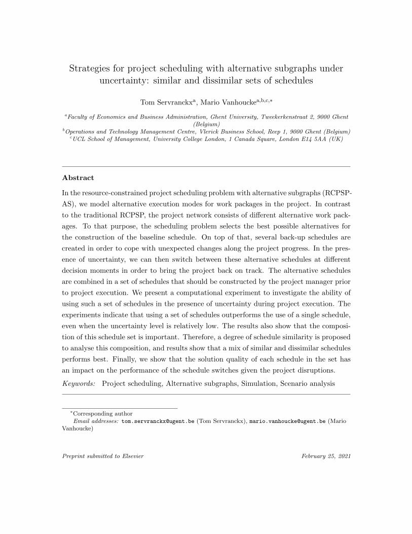
0.3. Alternative subgraphs

First, we will provide an overview of the existing literature on scheduling with alter-

natives. The aim is not to provide a complete literature overview, rather to highlight the

work that inspired this research. Then, we will briefly discuss the RCPSP followed by an

explanation of the RCPSP-AS as well as some problem-specific terminology.

The assumption that a project structure should be fixed and known beforehand has

been neglected in several research efforts from both a theoretical and practical point-of-

view. Logical constraints, such as OR- and BI-relations, are often used to model alterna-

tives. In the field of project scheduling, Vanhoucke and Coelho (2016) include OR- and

BI-relations in the RCPSP by converting them into standard AND-relations using a set of

transformation rules. Kis (2003) studies the job-shop scheduling problem with processing

alternatives (AJSP), where the routing of jobs consist of AND- and OR-subgraphs. In

order to solve disruption management problems, Kuster et al. (2008) model project struc-

tures with mutual exclusion relations between the activities to define options in case of

disruptions. Capek et al. (2012) extend the RCPSP with alternative process plans, while

Kellenbrink and Helber (2015) further extend the problem by splitting the logical and

precedence relations. Tao et al. (2018) discuss the RCPSP with hierarchical alternatives

and stochastic activity durations. Given the stochastic nature of the activity durations, the

problem is formulated using a stochastic chance constraint. Tao and Dong (2018) consider

6

alternative project structures in the multi-mode RCPSP (MRCPSP) with the objective of

minimising project makespan and total cost. Considering matrix-based project planning

problems, Kosztyan (2015) presents an exact algorithm to determine the optimal project

structure from a set of scenarios taking into account task importance and probability of

completion. In the field of assembly line balancing (ALB), a mathematical model (Capa-

cho and Pastor, 2006) and heuristic procedure (Capacho et al., 2009) for the assembly line

balancing problem with alternatives (ASALB) have been researched.

The basic RCPSP assigns start times to the activities in the project subject to prece-

dence and resource constraints. A directed acyclic graph G = (N,A) represents the

activity-on-the-node (AoN) project network with N the set of activities and A the set

of pairs of finish-to-start precedence related activities with zero minimum time lags. The

set N consists of a dummy start (end) activity 0 (n+ 1) and n non-dummy activities that

are characterised by an activity-specific duration di and a resource requirement ri,k for each

renewable resource type k ∈ Rρ. There are ak units of each resource type k available per

time interval, which is assumed deterministic and constant. The objective of the RCPSP

is to find a feasible schedule with a minimum makespan, i.e. a vector of start times si for

all the activities i ∈ N , that satisfies all precedence and resource constraints.

Where all activities i ∈ N should be scheduled in order to obtain a feasible schedule in

the basic RCPSP, this assumption is relaxed in the RCPSP-AS. In this problem, we dis-

tinguish between two types of activities: fixed activities and alternative activities. Where

fixed activities should always be present in a feasible schedule, only a selection of the alter-

native activities should be included in a feasible schedule. The alternative activities that

belong to the same selection subproblem are grouped in a so-called alternative subgraph.

An alternative subgraph is constructed of a set of mutually exclusive alternative branches

that thus consist of a subset of the alternative activities in the alternative subgraph. When

an alternative branch is selected in an alternative subgraph, this implies that the corre-

sponding set of alternative activities should be scheduled. The graph G thus consists of a

set of fixed activities Nf ⊆ N and a set of alternative activities Na ⊂ N that belong to

alternative branches. In Servranckx and Vanhoucke (2019), the sets of alternative activ-

ities that belong to an alternative branch are considered subgraphs G = (N ′, A′) with a

certain topological structure and resource characteristics. In table 1, we summarise the key

concepts of the RCPSP-AS and we illustrate them based on an example project structure

in figure 2. In summary, the RCPSP-AS is comprised of two subproblems: a selection and

a scheduling subproblem. The selection subproblem deals with the selection of alternative

7

activities such that the resulting project schedule is logical feasible. Logical feasibility

implies that exactly one alternative branch is selected for each alternative subgraph. The

scheduling subproblem identifies the optimal activity start times that satisfy the precedence

and resource constraints for the fixed and selected alternative activities. The objective of

the RCPSP-AS is to select and schedule the fixed and selected alternative activities with a

minimal project makespan such that the resulting project schedule is precedence, resource

and logical feasible.

Servranckx and Vanhoucke (2019) further extend the above problem formulation with

the definition of different types of alternative subgraphs based on the relations that are ob-

served between the alternative activities. Alternative subgraphs can be categorised in four

groups based on two dimensions: the presence of nested alternative subgraphs and linked

alternative branches. Both concepts are explained in more detail below and illustrated us-

ing the example projects in figure 1. In the remainder of this manuscript, a choice between

alternative branches in an alternative subgraph will always be illustrated by means of a

curved line ’)’.

Linked alternative branches: In case that alternative branches A and B are linked,

choosing alternative branch A implies that a part of alternative branch B also must be

executed. For example, the dotted line between the nodes 5 and 7 in Q2 shows a link

between both nodes. This link is modelled between two activities: one activity in node

5 and another activity in node 7. In case that node 5 is selected, the finish of the linked

activity in node 5 will start its successors in node 5 as well as the linked activity in node

7, which in turn will start its successors in node 7.

Nested alternative subgraph: In case that alternative subgraph C is nested in

alternative branch A, one alternative branch of alternative subgraph C must be selected

only if alternative branch A is selected. Otherwise, if alternative branch A is not selected,

none of the alternative branches of alternative subgraph C can be selected. A decision

between nodes 4 and 5 in Q3 should only be made when node 3 is selected. When node 2

would be selected, neither nodes 4 or 5 can be selected.

Based on these concepts, alternative subgraphs are categorised in four quadrants of a

two-by-two matrix, called the alternative subgraph matrix (ASM) in figure 1. The dichoto-

mous classification of alternative subgraphs as (non)linked and (non)nested is provided,

respectively, on the horizontal and vertical axis.

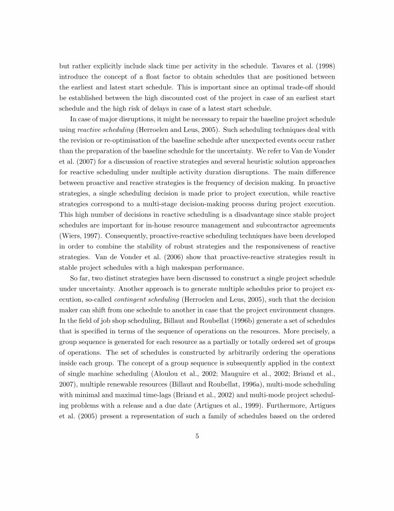
In the example project in figure 2, five work packages (WPs) need to be executed in

sequence and there exist alternative ways to execute WPs 1, 2 and 3. The choices between

8

No Yes

No

Yes

Nes

ted

alte

rnat

ive

subg

raph

s

Linked alternative branches

Non-linked nested project Linked nested project

Linked non-nested projectNon-linked non-nested project

2

3 6

5

S E1 4 7

2

3 6

5

S E1 4 7

Q1 Q2Q3 Q4

2

3 7

6

S E1 4 85

2

3 6

5

S E1 4 87

Alternativebranch A

Alternativebranch B

Alternativesubgraph C

Alternativebranch A

Figure 1: Alternative subgraph matrix (Servranckx and Vanhoucke, 2019)

alternatives for a WP are represented by means of a curved line ’)’ and alternative X in

WP Y is denoted by AX.Y. For example, there exist five alternative ways (A1.1 up to

A5.1) to execute WP 1 in figure 2. In order to keep the project structure comprehensible,

arcs are combined in junction points that are represented as �. An alternative subgraph

is a set of alternative execution modes for a WP and three such alternative subgraphs are

given in the example project: {A1.1,A2.1,A3.1,A4.1,A5.1}, {A1.2,A2.2,A3.2,A4.2,A5.2}and {A1.3,A2.3,A3.3}. Each of the alternative execution modes in an alternative subgraph

is called an alternative branch. For example, alternative subgraph {A1.2,A2.2,A3.2,A4.2,

A5.2} consists of five alternative branches. Each alternative branch is represented by a

node that corresponds with a subproject, e.g. figure 2 shows that node A5.2 consists of a

subproject with alternative activities. Since no alternative execution modes exist for WP 4

and WP 5, nodes A1.4 and A1.5 represent a subproject of fixed activities. Furthermore, we

observe that the alternative subgraph {A1.3,A2.3,A3.3} is nested in the alternative branch

A1.2. The dotted line between nodes A5.1 and A5.2 indicates a link between an activity

in alternative branch A5.1 and an activity in alternative branch A5.2. Linked alternative

branches can also exist within an alternative subgraph as is shown by the dotted line

between nodes A4.1 and A5.1. In the ASM, the example project would be classified as a

linked nested project (Q4).

The ASM allows us to unambiguously classify alternative subgraphs based on the afore-

mentioned dimensions and serves as a comprehensive overview that covers most alternative

subgraphs encountered in related literature. In order to solve problem instances of the

RCPSP-AS, Servranckx and Vanhoucke (2019) presented a tabu search (TS) in which the

9

Definition Explanation Illustration (see figure 2)

Fixed activity The inclusion of these activities All activities in the networkin the schedule is not optional of nodes A1.4 and A1.5

Alternative activity The inclusion of these activities E.g. activities in the networkin the schedule is optional as they of node A5.2belong to an alternative branch

Alternative branch Network of alternative activities E.g. the network of node A5.2 isAlternative subgraph Set of alternative branches from one of the five alternative branches

which a single alternative branch of the alternative subgraphshould be selected {A1.2,A2.2,A3.2,A4.2,A5.2}

Table 1: Definitions of the concepts of RCPSP-AS

S A1.1

A2.1

A3.1

A4.1

A5.1

A1.2

A2.2

A3.2

A1.3 A1.4 A1.5 E

A4.2

A5.2

A2.3

A3.3

Alternativebranch

Alternativesubgraph

Nested alternativesubgraph

Linked alternativebranches

Alternative activities

Fixed activities

link

AX.Y = Alternative X for WP Y

Figure 2: Illustrative example of a project with alternative subgraphs

strategies of different building blocks are guided by the position of problem instances in

the ASM in order to improve the performance of the search process.

0.4. Solution approach

This section presents the four-phased solution approach from initial schedule construc-

tion to final implementation of the switch between schedules in order to cope with the

project uncertainty. The four steps are briefly described in section 0.4.1 up to section

0.4.4, and an illustrative example is given in section 0.4.5.

0.4.1. Construct set of schedules

In step 1, we create a precedence, resource and logical feasible schedule for a problem

instance of the RCPSP-AS that consists of two subproblems. The first so-called selection

subproblem involves the selection of an alternative branch for each alternative subgraph.

In the second so-called scheduling subproblem, the selected activities should be scheduled

10

to obtain a precedence and resource feasible schedule with the lowest possible project

makespan. In this research, we generate the schedules using the TS procedure of Servranckx

and Vanhoucke (2019). A detailed review of the different building blocks of this procedure

is outside the scope of the current paper.

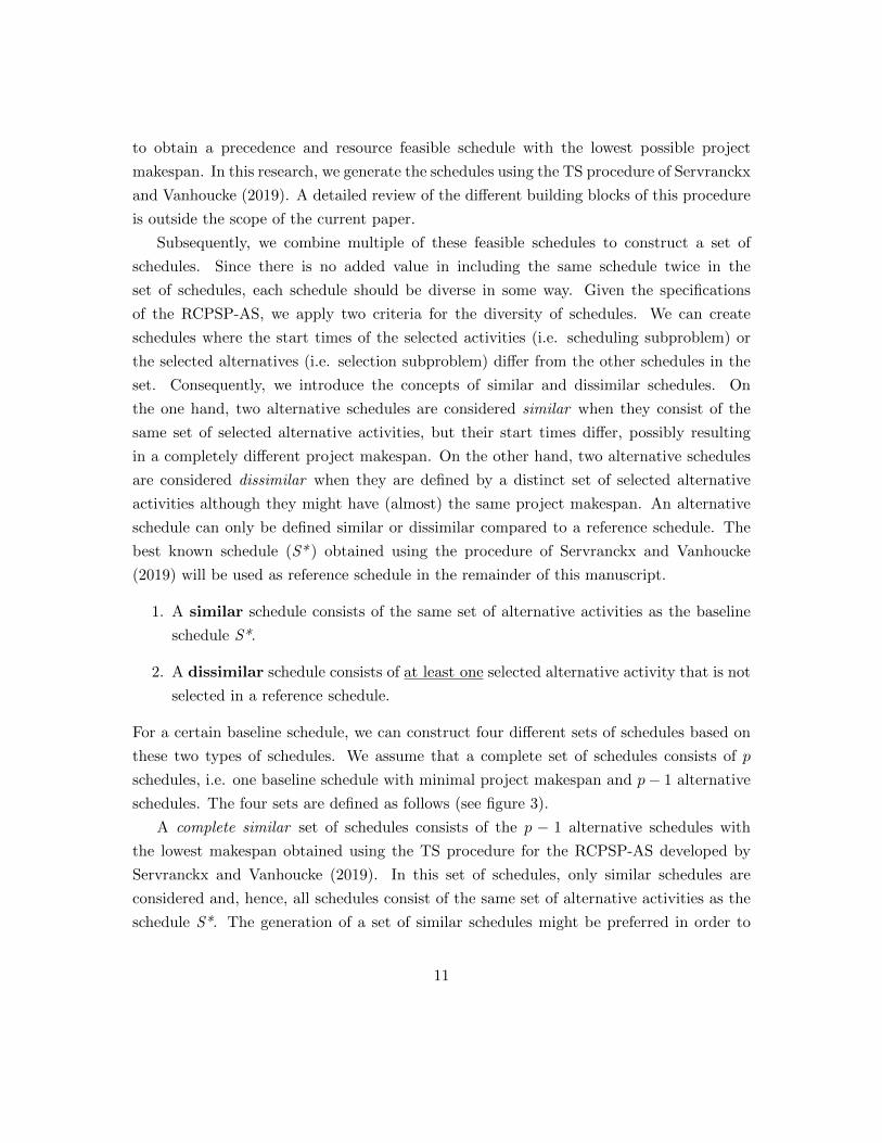
Subsequently, we combine multiple of these feasible schedules to construct a set of

schedules. Since there is no added value in including the same schedule twice in the

set of schedules, each schedule should be diverse in some way. Given the specifications

of the RCPSP-AS, we apply two criteria for the diversity of schedules. We can create

schedules where the start times of the selected activities (i.e. scheduling subproblem) or

the selected alternatives (i.e. selection subproblem) differ from the other schedules in the

set. Consequently, we introduce the concepts of similar and dissimilar schedules. On

the one hand, two alternative schedules are considered similar when they consist of the

same set of selected alternative activities, but their start times differ, possibly resulting

in a completely different project makespan. On the other hand, two alternative schedules

are considered dissimilar when they are defined by a distinct set of selected alternative

activities although they might have (almost) the same project makespan. An alternative

schedule can only be defined similar or dissimilar compared to a reference schedule. The

best known schedule (S* ) obtained using the procedure of Servranckx and Vanhoucke

(2019) will be used as reference schedule in the remainder of this manuscript.

1. A similar schedule consists of the same set of alternative activities as the baseline

schedule S*.

2. A dissimilar schedule consists of at least one selected alternative activity that is not

selected in a reference schedule.

For a certain baseline schedule, we can construct four different sets of schedules based on

these two types of schedules. We assume that a complete set of schedules consists of p

schedules, i.e. one baseline schedule with minimal project makespan and p− 1 alternative

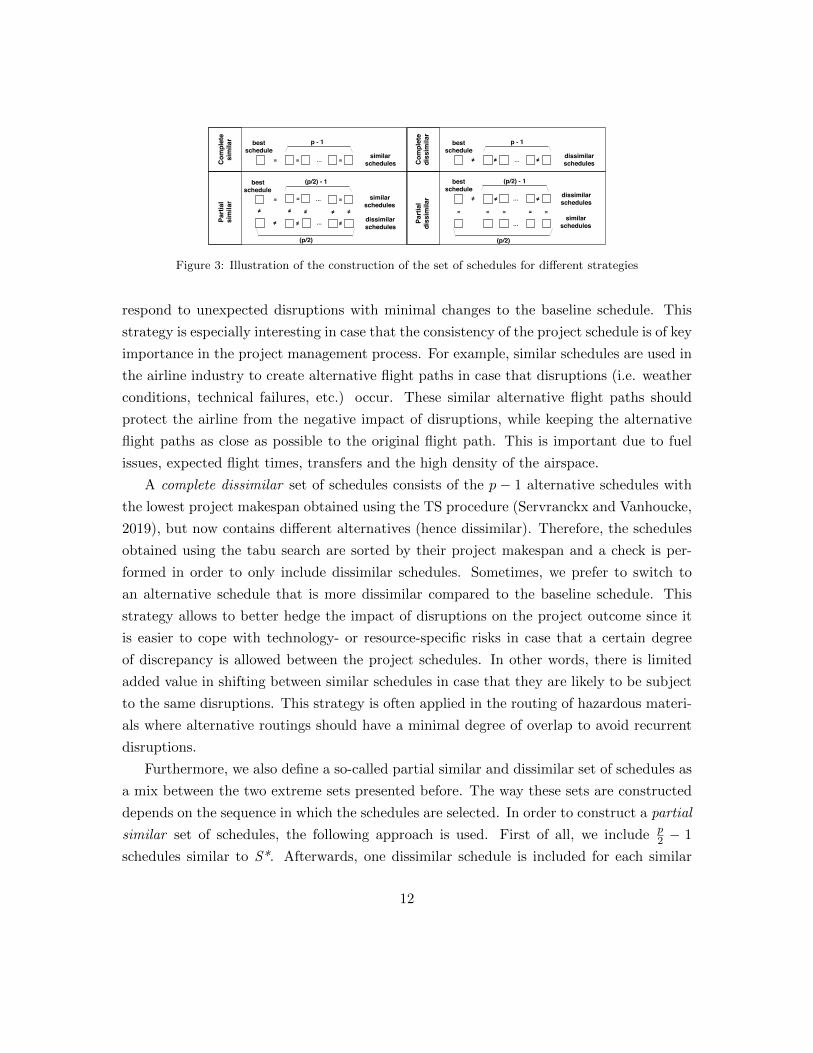
schedules. The four sets are defined as follows (see figure 3).

A complete similar set of schedules consists of the p − 1 alternative schedules with

the lowest makespan obtained using the TS procedure for the RCPSP-AS developed by

Servranckx and Vanhoucke (2019). In this set of schedules, only similar schedules are

considered and, hence, all schedules consist of the same set of alternative activities as the

schedule S*. The generation of a set of similar schedules might be preferred in order to

11

Part

ial

sim

ilar

best schedule

…

(p/2) - 1

…

similar schedules

dissimilarschedules

Part

ial

diss

imila

r

best schedule

…

(p/2) - 1

…

dissimilarschedules

similarschedules

Com

plet

esi

mila

r

Com

plet

edi

ssim

ilar

best schedule

…

p - 1

similar schedules

best schedule

…

p - 1

dissimilarschedules= = = ≠ ≠ ≠

≠ ≠ ≠ ≠ ≠

≠ ≠ ≠= = =

= = = = =

≠ ≠ ≠

(p/2) (p/2)

Figure 3: Illustration of the construction of the set of schedules for different strategies

respond to unexpected disruptions with minimal changes to the baseline schedule. This

strategy is especially interesting in case that the consistency of the project schedule is of key

importance in the project management process. For example, similar schedules are used in

the airline industry to create alternative flight paths in case that disruptions (i.e. weather

conditions, technical failures, etc.) occur. These similar alternative flight paths should

protect the airline from the negative impact of disruptions, while keeping the alternative

flight paths as close as possible to the original flight path. This is important due to fuel

issues, expected flight times, transfers and the high density of the airspace.

A complete dissimilar set of schedules consists of the p − 1 alternative schedules with

the lowest project makespan obtained using the TS procedure (Servranckx and Vanhoucke,

2019), but now contains different alternatives (hence dissimilar). Therefore, the schedules

obtained using the tabu search are sorted by their project makespan and a check is per-

formed in order to only include dissimilar schedules. Sometimes, we prefer to switch to

an alternative schedule that is more dissimilar compared to the baseline schedule. This

strategy allows to better hedge the impact of disruptions on the project outcome since it

is easier to cope with technology- or resource-specific risks in case that a certain degree

of discrepancy is allowed between the project schedules. In other words, there is limited

added value in shifting between similar schedules in case that they are likely to be subject

to the same disruptions. This strategy is often applied in the routing of hazardous materi-

als where alternative routings should have a minimal degree of overlap to avoid recurrent

disruptions.

Furthermore, we also define a so-called partial similar and dissimilar set of schedules as

a mix between the two extreme sets presented before. The way these sets are constructed

depends on the sequence in which the schedules are selected. In order to construct a partial

similar set of schedules, the following approach is used. First of all, we include p2 − 1

schedules similar to S*. Afterwards, one dissimilar schedule is included for each similar

12

schedule in the set of schedules, which results in a total of p2 dissimilar schedules. During the

generation of these schedules, the procedure makes sure that the set of dissimilar schedules

are also mutually dissimilar. A likewise, but opposite, approach is used in order to construct

a partial dissimilar set of schedules. First, we include p2 − 1 schedules dissimilar to S* and

mutually dissimilar to each other. Afterwards, one similar schedule for each dissimilar

schedule is included in the set resulting in a total of p2 similar schedules. Each time

different schedules are generated, the one with the lowest possible makespan is selected.

During project execution, only one schedule can be selected at each point in time. In

case of unexpected disruptions, however, the project manager can switch between alter-

native schedules in the set of schedules. Consequently, the ability of the set of schedules

to deal with uncertainty depends on the characteristics of the alternative schedules that

together comprise the set of schedules.

0.4.2. Model uncertainty

In step 2, we simulate uncertainty during project execution in order to evaluate the

ability of each set of schedules to cope with uncertainty. We consider three types of uncer-

tainty and each of them can occur at different stages of the project (stages of uncertainty).

Types of uncertainty. We differentiate between three types of uncertainty: duration vari-

ability, resource breakdowns and resource efficiencies. We will briefly discuss each type of

uncertainty:

Duration variability (DV) In order to simulate uncertain activity durations, we

draw the actual duration for each activity i as a discretised value from a right-skewed beta

distribution. The distribution is modelled by two positive shape parameters α = 2 and

β = 5 and a mean duration equal to the planned duration di (Van de Vonder et al., 2008).

Resource breakdown (RB) Although machine breakdowns are well-studied in ma-

chine and job-shop scheduling, uncertain resource availabilities are seldom included in

simulation studies for the RCPSP and its variants. The approach of Lambrechts et al.

(2008) to model stochastic resource breakdowns is applied in this paper. The increase in

duration of an activity due to resource breakdowns is determined by the number of re-

source breakdowns of the resources that are required by an activity and the repair time

related to each resource breakdown. We define the mean time to failure MTTFk and the

mean time to repair MTTRk for each resource type k in order to simulate the impact of

resource breakdowns. We draw the values for the time to the next failure and the time

13

to repair that failure from an exponential distribution with the rate parameter equal to,

respectively, 1/MTTFk and 1/MTTRk. The value for the MTTFk and MTTRk are de-

termined based on the project deadline, which is equal to the makespan of the best known

schedule obtained using the procedure of Servranckx and Vanhoucke (2019). We assume

that the resource availability of resource type k is set equal to zero during a breakdown.

Resource efficiency (RE) In the baseline schedule, a normal (i.e. 100%) resource

efficiency of resource type k (rek) is assumed, which implies that activity j can be executed

in di time units using ri,k resource units. During project execution, however, the resource

efficiency might be higher (rek > 100%) or lower (rek < 100%) than expected in the

baseline schedule. The actual activity duration (di) will be equal to the ratio of the planned

activity duration (di) over the weighted average efficiency of the resource types k that are

required by this activity, i.e. di = diwavgk{rek} . Since resources should work together on the

activity, the activity duration is calculated using a weighted average resource efficiency. As

an example, an activity i with di = 9 and a resource use ri,1 = 1 and ri,2 = 2 as well as a

resource efficiency re1 = 0.85 and re2 = 0.95 faces a weighted average resource efficiency

equal to 91,67% (=0.85 ∗ 1 + 0.95 ∗ 2

3). Consequently, the actual activity duration di is

equal to 10 days (= 90.9167).

Stages of uncertainty. We define three stages of uncertainty that determine in which stages

of the project the uncertainty is concentrated. We simulate that (1) the uncertainty is

higher in the early stages of the project, (2) the uncertainty is equally distributed over the

project horizon and (3) the uncertainty is higher in the late stages of the project.

0.4.3. Evaluate switch options

Given the simulated project execution, it might be preferred to switch between alter-

native schedules in order to minimise the actual project makespan. In step 3, we analyse

such a switch between alternative schedules, which consists of two components to determine

when and how we can switch between alternative schedules.

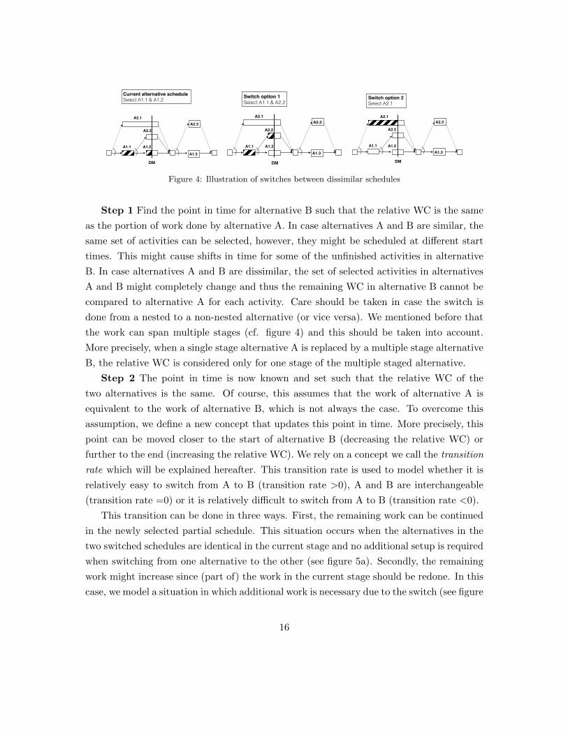
Decision moments (when to switch) Switches between alternative schedules are

implemented at milestones or decision moments (DMs) during project execution. When

an alternative schedule is switched, the partial schedule from the DM up to the end of

the project is replaced by the partial schedule of another schedule such that the resulting

complete project schedule is again resource and logical feasible. This implies that the infor-

mation with respect to the scheduling priorities as well as the set of selected alternatives in

14

the newly selected alternative schedule will be used to complete the current partial sched-

ule. In this study, we will relate the DMs to the stages, as implemented by Servranckx and

Vanhoucke (2019), in the project. A stage comprises a work package in the project that

might consist of alternative execution modes. However, certain alternative branches in a

project instance might span multiple stages in the project due to the existence of nested

alternatives (see section 0.3). Figure 4 graphically displays a project with three stages Y

and two alternatives X per stage, denoted by AX.Y. Normally, work packages should be

executed sequentially and, therefore, the project is divided into different stages. However,

some work can be assembled in a bigger package and executed over multiple stages. Alter-

native 2.1 is such an example and covers stages 1 and 2. It is an alternative for the work of

A1.1 and the work of one of its successors (A1.2 or A2.2). A first decision must be made

at stage 1 by selecting either A1.1 or A2.1. If A2.1 is selected, no further decision must be

made at stage 2. However, since A1.2 and A2.2 are nested in A1.1, selecting A1.1 requires

a second decision at stage 2 (either A1.2 or A2.2).

When we relate the DMs to the stages in the project, two distinct situations are defined.

First, each DM can be set after the completion of a stage in the project. This means that

no alternatives will be in progress, and switching is only possible when a stage has just

finished and the next stage has not started yet. This corresponds to a practical situation

in which the decision maker has to commit to past decisions and can only intervene in the

project when the results of past decisions are realised. Secondly, the DM can be set within

stages, which means that the decision maker must consider an intervention in the project

when work is in progress during the current stage.

Transition (how to switch) At a certain DM, a switch must be made between

alternative A and a new alternative B. As mentioned, alternative A can be in progress (DMs

within stages) or completely finished (DMs after stages). When performing such a switch,

the portion of the work that is already completed in alternative A will be calculated using

the concept of work content (WC) (equal to activity duration multiplied by its resource

requirements). Consequently, the portion of work done is equal to the work of the finished

activities and the completed work of the activities in progress divided by the total WC of

all activities in alternative A.

When switching from alternative A to alternative B, not all the work in alternative B

must be done. Therefore, it is important to determine what portion of the work is assumed

completed in alternative B, and what portion should still be done. Therefore, we use the

following two-step approach:

15

DM

Current alternative scheduleSelect A1.1 & A1.2

Switch option 1Select A1.1 & A2.2

A2.1

A1.1

A2.2

A1.2

DM

DM

Switch option 2Select A2.1

A2.1

A1.1

A2.2

A1.2

A2.1

A1.1

A2.2

A1.2

A2.3

A1.3

A2.3

A1.3

A2.3

A1.3

DM

Current alternative scheduleSelect A1.1 & A1.2

Switch option 1Select A1.1 & A2.2

A2.1

A1.1

A2.2

A1.2

DM

DM

Switch option 2Select A2.1

A2.1

A1.1

A2.2

A1.2

A2.1

A1.1

A2.2

A1.2

A2.3

A1.3

A2.3

A1.3

A2.3

A1.3

DM

Current alternative scheduleSelect A1.1 & A1.2

Switch option 1Select A1.1 & A2.2

A2.1

A1.1

A2.2

A1.2

DM

DM

Switch option 2Select A2.1

A2.1

A1.1

A2.2

A1.2

A2.1

A1.1

A2.2

A1.2

A2.3

A1.3

A2.3

A1.3

A2.3

A1.3

Figure 4: Illustration of switches between dissimilar schedules

Step 1 Find the point in time for alternative B such that the relative WC is the same

as the portion of work done by alternative A. In case alternatives A and B are similar, the

same set of activities can be selected, however, they might be scheduled at different start

times. This might cause shifts in time for some of the unfinished activities in alternative

B. In case alternatives A and B are dissimilar, the set of selected activities in alternatives

A and B might completely change and thus the remaining WC in alternative B cannot be

compared to alternative A for each activity. Care should be taken in case the switch is

done from a nested to a non-nested alternative (or vice versa). We mentioned before that

the work can span multiple stages (cf. figure 4) and this should be taken into account.

More precisely, when a single stage alternative A is replaced by a multiple stage alternative

B, the relative WC is considered only for one stage of the multiple staged alternative.

Step 2 The point in time is now known and set such that the relative WC of the

two alternatives is the same. Of course, this assumes that the work of alternative A is

equivalent to the work of alternative B, which is not always the case. To overcome this

assumption, we define a new concept that updates this point in time. More precisely, this

point can be moved closer to the start of alternative B (decreasing the relative WC) or

further to the end (increasing the relative WC). We rely on a concept we call the transition

rate which will be explained hereafter. This transition rate is used to model whether it is

relatively easy to switch from A to B (transition rate >0), A and B are interchangeable

(transition rate =0) or it is relatively difficult to switch from A to B (transition rate <0).

This transition can be done in three ways. First, the remaining work can be continued

in the newly selected partial schedule. This situation occurs when the alternatives in the

two switched schedules are identical in the current stage and no additional setup is required

when switching from one alternative to the other (see figure 5a). Secondly, the remaining

work might increase since (part of) the work in the current stage should be redone. In this

case, we model a situation in which additional work is necessary due to the switch (see figure

16

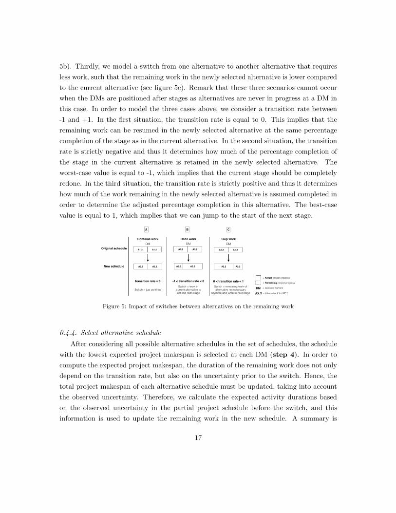
5b). Thirdly, we model a switch from one alternative to another alternative that requires

less work, such that the remaining work in the newly selected alternative is lower compared

to the current alternative (see figure 5c). Remark that these three scenarios cannot occur

when the DMs are positioned after stages as alternatives are never in progress at a DM in

this case. In order to model the three cases above, we consider a transition rate between

-1 and +1. In the first situation, the transition rate is equal to 0. This implies that the

remaining work can be resumed in the newly selected alternative at the same percentage

completion of the stage as in the current alternative. In the second situation, the transition

rate is strictly negative and thus it determines how much of the percentage completion of

the stage in the current alternative is retained in the newly selected alternative. The

worst-case value is equal to -1, which implies that the current stage should be completely

redone. In the third situation, the transition rate is strictly positive and thus it determines

how much of the work remaining in the newly selected alternative is assumed completed in

order to determine the adjusted percentage completion in this alternative. The best-case

value is equal to 1, which implies that we can jump to the start of the next stage.

= Actual project progress

= Remaining project progress

DM = Decision moment

AX.Y = Alternative X for WP Y

A1.2

A2.2 A2.2

A1.2Original schedule

New schedule

DMSkip work

= Actual project progress

= Remaining project progress

DM = Decision moment

AX.Y = Alternative X for WP Y

Switch = remaining work of alternative not necessary

anymore and jump to next stage

A1.2

A2.2 A2.2

A1.2

DMRedo work

Switch = work in current alternative is lost and redo stage

-1 < transition rate < 0

A1.2

A2.2 A2.2

A1.2

DMContinue work

Switch = just continue

transition rate = 0 0 < transition rate < 1

A B C

Figure 5: Impact of switches between alternatives on the remaining work

0.4.4. Select alternative schedule

After considering all possible alternative schedules in the set of schedules, the schedule

with the lowest expected project makespan is selected at each DM (step 4). In order to

compute the expected project makespan, the duration of the remaining work does not only

depend on the transition rate, but also on the uncertainty prior to the switch. Hence, the

total project makespan of each alternative schedule must be updated, taking into account

the observed uncertainty. Therefore, we calculate the expected activity durations based

on the observed uncertainty in the partial project schedule before the switch, and this

information is used to update the remaining work in the new schedule. A summary is

17

graphically displayed in figure 6. The calculation of the expected project makespan is done

according to the following rules:

Duration variability The variability in the durations of activities prior to the DM is

taken into account to estimate the future activity variability. In case that the completed ac-

tivities were finished ahead of schedule, the remaining activity durations will be decreased,

which possibly results in a lower project makespan. In case that the completed activities

were finished late, the remaining activity durations will be increased, which might result

in a higher project makespan than initially expected. In figure 6a, we assume that the

average activity duration in alternatives A1.1, A2.2 and A2.3 prior to DM is 50% higher

than the planned activity duration. Since we expect a similar duration variability in the

future project execution, the planned duration of the remaining work in A2.3 as well as

the planned duration of the total work in A3.4 and A1.5 is increased with 50%.

Resource breakdown The average downtime of a resource up to DM is used to

calculate an updated duration for all remaining activities that make use of this resource.

In case an activity requires multiple resources, the maximum downtime of these resources

is used to update the expected activity duration. In figure 6b, we assume a downtime of

resource type 2 in A2.2 and A2.3 prior to DM equal to 20%, while no downtime in resource

type 1 occurs during the completion of A1.1. In case that we assume that resource type 2

is also used in A2.3, we expect a 20% downtime during the remaining work for A2.3.

Resource efficiency The resource efficiency prior to DM is used to update the ex-

pected resource efficiency, which results in an expected makespan that can differ from the

one initially planned. In figure 6c, it is assumed that the resource efficiency of resource

type 1 in A1.1 is equal to 75%. In case that A1.5 also makes use of resource type 1, its

planned duration should be multiplied by 1.33 (= 10.75). Similarly, we can calculate the

expected duration of the remaining work in A2.3, assuming that it makes use of resource

type 2, given that the resource efficiency of resource type 2 is equal to 63% in A2.2 and

A2.3.

Every time the current alternative schedule is switched, the expected project makespan

of the alternative schedules in the set is calculated along the previous rules. Then, the

alternative schedule with the shortest expected project makespan is selected and replaces

the current schedule. If an alternative schedule has the same expected makespan as the

current schedule, we retain the current schedule. In case that two alternative schedules

have the same expected project makespan (lower than the expected project makespan of

the current schedule), we select the one that is most similar to the current schedule.

18

Stages

TimeDM Expected

project makespan

A1.1

A2.2

A 2.3

A3.4

Resourceefficiency: 75%

Resourceefficiency: 63%

A1.5

DM = Decision momentAX.Y = Alternative X

for WP Y

Stages

TimeDM Expected

project makespan

Stages

DM Expectedproject

makespan

Average downtime: 20%

A1.1

A2.2

A 2.3

A3.4

A1.5

A1.1

A2.2

A2.3

A3.4

A1.5Time

Average durationvariability: 50%

B C

Stages

TimeDM Expected

project makespan

Stages

DM Expectedproject

makespan

Average downtime: 20%

A1.1

A2.2

A 2.3

A3.4

A1.5

A1.1

A2.2

A2.3

A3.4

A1.5Time

Average durationvariability: 50%

A

Figure 6: Examples on updating alternative schedules for three types of uncertainty

0.4.5. Illustrative example

Figure 7 illustrates the four-step solution approach based on an example project that

consists of five WPs in sequential stages. For each WP Y, there exist three alternatives,

denoted by A1.Y, A2.Y and A3.Y. Assume that the selection of alternatives that results

in the lowest project makespan for the project example is represented by S1.0. In the

remainder of this section, we will discuss the four steps of the solution approach based on

the illustrative example in figure 7.

Step 1 Based on the best schedule S1.0, four sets of six schedules are constructed

using the different strategies discussed in section 0.4.1. On the one hand, similar schedules

with respect to S1.0 consist of the same set of selected alternatives and, therefore, they

are denoted by SX.Y with X = 1 and Y = {1, 2, 3, 4, 5}. On the other hand, dissimilar

schedules with respect to S1.0 are denoted by SX.Y with X = {2, 3, 4, 5, 6} and Y = 0

since they consist of a different set of selected alternatives. For example, S1.1 (S2.0) is a

similar (dissimilar) schedule compared to S1.0. Given these (dis)similar schedules, we can

construct four sets of schedules, i.e. partial and complete (dis)similar schedules (figure 7).

Step 2 After having constructed the set of schedules, we initiate the project execution

according to the best schedule of the set of schedules (S1.0). The execution of the project

is simulated up to a decision moment (DM) using the three types of uncertainty (section

0.4.2) and thus the activities prior to DM might be subject to disruptions. Assume that

the first DM is set after completing 100% of the work of A1.1 and 50% of the work of A2.2.

Step 3 Given the uncertainty during project execution, we have to analyse whether it

is preferred to continue with S1.0 or switch to an alternative schedule. Therefore, we will

evaluate the switches between the different alternative schedules as discussed in section

0.4.3. Let us assume that we make use of a complete dissimilar set (set 4). In figure 7,

we display a switch from S1.0 to S2.0 at DM. First, we have to interrupt A2.2 in S1.0 at

DM and continue with A1.2 in S2.0. Subsequently, a transition is required with a positive,

19

Uncertainty:

1. Duration variability 2. Resource unavailability 3. Resource inefficiency

Stages

Time

12345

DM

A1.1

A2.3 A3.4

A1.5

S1.0

Number of decision moments

Step 2 Model uncertainty

A2.2

Step 1 Construct set of schedules

S1.0

S2.0

S4.0S5.0

S6.0

S3.0

Complete dissimilar

Set 4

S1.1

S1.0

S1.2

S1.3

S1.4

S1.5

Complete similar

Set 1

S1.0

S1.1

S2.1S3.0

S3.1

S2.0

Partialdissimilar

Set 3

S2.0

S3.0

S4.0

S5.0

S6.0

A1.1 A1.2 A2.3 A2.4 A3.5A2.1 A1.2 A1.3 A3.4 A1.5

A1.1 A2.2 A2.3 A1.4 A2.5

A2.1 A3.2 A2.3 A2.4 A3.5

A3.1 A1.2 A1.3 A2.4 A3.5

set of schedules

Best schedule S1.0Stages

Time

12345

A1 .1A2.2

A2.3A3.4

A1.5

A1.1

1 2 3 4 5

AX.Y = Alternative X for WP Y

A2.1

A3.1

A1.2

A2.2

A3.2

A1.3

A2.3

A3.3

A1.4

A2.4

A3.4

A1.5

A2.5

A3.5

Single schedule

S1.0

S2.0

S1.1

S3.0S1.2

S4.0

Partialsimilar

Set 2

Stages

Time

12345

DM

A1.1 A1.2

A2.3A2.4

A3.5Transition rate = 50%

Step 3 Evaluate switch options Step 4 Select alternative schedule

S1.0current

switch

S2.0 S3.0 S4.0 S5.0 S6.0 Set 4

S1.0 S2.0

1

DM

DM

DM

2

Switch

expected progress

Stages

Time

12345

DM

A1.1

A2.3 A3.4

A1.5

A2.2

current progress

S1.0current

switch

S2.0 S3.0 S4.0 S5.0 S6.0 Set 4

S1.0 S2.0

Switch from S1.0 to S2.0

A2.2

A1.2

A1.2

Figure 7: Overview of the solution approach

neutral or negative transition rate since a switch between dissimilar schedules is modelled.

Let us assume a transition rate equal to -0.5, which implies that 50% of the work executed

in A2.2 at DM should be redone in A1.2.

Step 4 At DM, the past project progress is used to update the expected future project

progress and, subsequently, the best alternative schedule in the set of schedules should be

selected (section 0.4.4). In case that we consider the complete dissimilar set of schedules,

the expected project makespan of the current schedule S1.0 is compared to the expected

project makespan of the alternative schedules S2.0 up to S6.0. After evaluation, we will

switch to the alternative schedule SX.0 with the lowest expected project makespan at DM.

0.5. Computational experiments

In section 0.5.1, we briefly review the design of the network instances used in the ex-

periments as well as discuss the different uncertainty parameters used in this research.

Subsequently, we investigate the performance of the different strategies under various sim-

ulation settings in section 0.5.2. More precisely, we investigate the construction of the

schedule set, the impact of uncertainty and the problem features in our solution approach.

20

The computational experiments in this study were carried out on a computer with an Intel

Core i5 processor 2.5 GHz and 8 Gb RAM.

0.5.1. Experimental design

Network instances. Servranckx and Vanhoucke (2019) have developed a dataset that con-

sists of 36,000 data instances for the RCPSP-AS. For each unique combination of parameter

settings, the authors generated 10 project instances in the dataset. In our computational

experiments, we consider the first of those 10 instances, which results in a total of 3,600

test instances. The project instances of the RCPSP-AS are characterised by project and

flexibility parameters. On the one hand, two project parameters are considered to describe

the structure of the project network: the resource constraindness (RC) and serial-parallel

(SP) indicator. The RC and SP indicators are set equal to 0.25, 0.5 or 0.75 in the dataset

of Servranckx and Vanhoucke (2019). On the other hand, the flexibility parameters are

briefly discussed in the remainder of this section.

Percentage flexibility (%flex) This parameter determines the number of alternatives

in the project structure and, consequently, a higher percentage flexibility allows for a larger

differentiation between the complete similar and dissimilar set of schedules. Each instance

consists of five stages and each stage has a maximum of five alternatives per stage. The

actual number of alternatives is determined as 25%, 50%, 75% and 100% of the maximum

number of alternatives (i.e. equal to 25) in the project.

Percentage nested (%nested) This parameter regulates the number of alternative

subgraphs that are embedded in one another. The actual number of nested alternative

subgraphs can be determined as a percentage (i.e. 0%, 25%, 50%, 75% and 100%) of the

number of alternative subgraphs that can potentially be nested.

Percentage linked (%linked) This parameter determines the number of alternative

branches that are connected such that the selection of one alternative branch implies the

partial selection of another alternative branch. The actual number of linked alternative

branches can be determined as a percentage (i.e. 0%, 25%, 50%, 75% and 100%) of the

number of alternative branches that can potentially be linked.

Flexibility distribution This parameter determines how the alternatives are dis-

tributed over the different stages in the project. Servranckx and Vanhoucke (2019) dis-

tinguish between an early, middle, late and a uniform focus. This implies that a pre-

determined number of alternatives (potentially nested or linked) can be positioned mainly

in the first, middle or last stages of the project or can be uniformly distributed over the

21

five stages in the project horizon.

A detailed explanation of the data generation procedure is outside the scope of the

current paper, however, we refer to the work of Servranckx and Vanhoucke (2019).

Parameters of simulation experiment. In this section, the parameter settings of the sim-

ulation study introduced in section 0.4 are summarised in table 2. We categorise the

parameters in three groups: the parameters to create the set of schedules, the uncertainty

parameters and the decision-making parameters.

The construction of the set of schedules depends on the size of the set of schedules and

the number of similar and dissimilar schedules. The number of alternative schedules varies

between 4 and 20. The number of similar and dissimilar schedules in the set of schedules

varies to define complete (dis)similar and partial (dis)similar sets of schedules.

The uncertainty parameters are used to model the types of uncertainty and the stages

of uncertainty. First of all, the three types of uncertainty are modelled using parameters

that are summarised in table 2. For each parameter, three different values are chosen,

and we labelled them as low, medium or high uncertainty. The duration variability is

modelled using a right-skewed beta distribution that is transformed such that the mean

duration of activity i is equal to the planned duration di, independent of a low, medium

or high uncertainty. Table 2 shows the percentage of di that is used as minimum or

maximum duration in the skewed beta distribution for low, medium and high uncertainty

levels. For the resource breakdowns, the values for MTTFk and MTTRk are expressed as

a percentage of the project deadline. The resource efficiency of resource type k is drawn

from a triangular distribution with a minimum and maximum value, respectively, equal to

0.25 and 0.75, independent of a low, medium or high uncertainty. However, the expected

resource efficiency is different for the three risk levels as shown in table 2.

Based on the stochastic parameters discussed before, we can model the number of

disruptions of each type that are expected during project execution. In this research,

we want to model disruptions occurring in different stages of the project execution. We

distinguish between three cases: (1) early focus, (2) uniform distribution and (3) late focus.

To that purpose, we subdivide the project execution is three stages. Then, a probability

is defined for each stage in each of the three cases: (1) 75%-50%-25%, (2) 50%-50%-50%

and (3) 25%-50%-75%. These values determine the probability that a disruption modelled

using the above stochastic parameters will actually occur during project execution.

We define two decision-making parameters. First, the number of decision moments

22

determines when switches between schedules are possible. Secondly, the overlap of work

between two switched schedules is modelled by the transition rate. The number of DMs

is set to 5, 10 or 20. In case of five DMs, each DM will be included after a stage in

the project since the data instances of Servranckx and Vanhoucke (2019) consist of five

stages. When there are more than five DMs, the DMs are included within the stages. For

example, a total of 20 DMs will result in four DMs per stage (i.e. at 20%, 40%, 60% and

80% completion of a stage). In case that there are DMs within stages, the transition rate

should be used to model how work in one alternative is transferred to another alternative.

In our research, this transition rate varies between -1 and +1 in steps of 0.5. In a practical

setting, the size of the transition rate (either positive, neutral or negative) is not known

prior to project execution and only observed at the DMs. In our research, we also assume

that the transition rate at each DM is unknown to the decision maker in order to avoid

that the impact of future switches is anticipated in the simulation experiment.

Parameters for the set of schedules

Number of alternative schedules (p) 4, 6, 8, 10, 20Number of dissimilar schedules 0, p

2 , p2 − 1, p− 1

Uncertainty parameters

Types of uncertainty Low Medium HighDuration variability (DV)

Minimum duration 0.75 0.5 0.25Maximum duration 1.625 2.25 2.875

Resource breakdown (RB)MMTFk 1 3 5MMTRk 0.5 1 1.5

Resource efficiency (RE) 0.75 0.5 0.25Stages of uncertainty Early Uniform LateProbability - first stages 0.75 0.5 0.25Probability - middle stages 0.5 0.5 0.5Probability - last stages 0.25 0.5 0.75

Decision-making parameters

Number of decision moments 5, 10, 20Transition rate -1, -0.5, 0, 0.5, 1

Table 2: Summary of parameter settings

0.5.2. Computational results

The computational experiments are conducted in three blocks using the network and

uncertainty parameters presented in section 0.5.1. In table 3, we summarise the parameter

settings for the experiments that are discussed in the following sections. More precisely, we

23

Schedule set Uncertainty

Size set Procedure1 Initial2 Types uncertainty3 Decision moments Transition rate Degree uncertainty4 Stage uncertainty5

Table 4 (1,4,6,8,10,20) TS R (DV,RB,RE) 5,10,20 0 M UTable 5 10 TS/MSILS R (DV,RB,RE) 5,10,20 -1,0.5,0,0.5,1 L,M,H UTable 6 10 TS R/P ALL 5,10,20 -1,0.5,0,0.5,1 M UTable 7 10 TS R (DV,RB,RE) 5,10,20 -1,0.5,0,0.5,1 M UFigure 8a 1,10 TS R (DV,RB,RE) 5,10,20 -1,0.5,0,0.5,1 L,M,H E,U,LTable 8 10 TS R (DV,RB,RE) 5,10,20 -1,0.5,0,0.5,1 M U

Problem featuresProject instances with a %flex equal to 0.25, 0.5, 0.75 and 1 are considered in the computational experimentsProject instances with a %nested and %linked equal to 0, 0.25, 0.5, 0.75 and 1 are considered in the computational experimentsProject instances with an early, middle, late and uniform flexibility distribution are considered in the computational experimentsLegend:1In the experiments, the set of schedules is generated using the tabu search (TS) or multi-start iterated local search (MSILS)proposed by Servranckx and Vanhoucke (2019).2The initial schedule to start the project execution is selected using a proactive (P) or reactive (R) approach.3ALL: all 7 combinations of the three uncertainty types (DV, RB and RE) discussed in table 24 Low (L), medium (M) and high (H) degree of uncertainty modelled using the parameter settings of table 25 Early (E), uniform (U) and late (L) stage of uncertainty modelled using the probabilities in table 2

Table 3: Summary of the parameter settings from table 2 in the computational experiments

specify the values of the parameters in table 2 that are used in the experiments discussed in

table 4 up to table 8 and figure 8. The key parameters that are the focus of each experiment

are highlighted in bold.

Schedule set. First of all, we investigate the impact of the size of the set of schedules

on the actual project makespan. When the size of the set is equal to 1, we consider a

single schedule rather than a set of schedules. This allows us to analyse the added value

of using multiple alternative schedules in order to cope with uncertainty. Note that a

minimum of four schedules is required in a set of schedules in order to distinguish between

the different strategies discussed in section 0.4.1. In table 4, we show the average actual

project makespan for different sizes of the set of schedules, subdivided by the different

strategies. The size of the set that results in the lowest project makespan is indicated in

bold. Since switches between alternative schedules are not possible in case that only a

single schedule is available, we should cancel out the effect of the transition rate in order to

ensure a fair comparison between the multiple and single schedule approach. Therefore, we

compare the performance of the four strategies at a transition rate equal to zero with the

performance of a single schedule. The computational experiment shows that, on average,

the use of multiple schedules results in a lower actual project makespan compared to a single

schedule. In case that multiple schedules are considered, we observe a small difference in

performance between the different sizes. This observation could be explained by the fact

that the best alternative schedules are first included in the set and, consequently, the

alternative schedules that are added later only provide an incremental improvement of the

24

Different Size of the set of schedulesstrategies 1 4 6 8 10 20

Single schedule 263.92 - - - - -Complete dissimilar - 226.94 223.83 223.13 221.32 225.76Partial dissimilar - 228.08 224.16 222.02 220.89 219.89Partial similar - 236.37 232.61 233.06 235.62 235.76Complete similar - 257.31 258.36 261.06 259.56 259.71

Average 263.92 237.18 234.74 234.82 234.35 235.28

Table 4: Average actual project makespan for different sizes of the set of schedules

quality of the set. However, a limited size of the set of schedules has a negative impact on

the actual project makespan. In summary, the number of alternative schedules should be

large enough to provide sufficient decision-making options, yet small enough to allow the

decision maker to manage the set of schedules. Given that a set of schedules is preferred

over a single schedule, we investigate the impact of the quality of the schedules in the set

on the performance of the solution approach. Therefore, we will compare our approach

with high-quality schedules generated using the TS procedure (Servranckx and Vanhoucke,

2019) with a benchmark approach that generates lower-quality schedules. More precisely,

we will use the MSILS (Servranckx and Vanhoucke, 2019) to construct the set of schedules.

Similar to the use of the TS in our approach, the MSILS will be used to generate a total

of 5,000 schedules and, subsequently, the 10 best similar and dissimilar schedules will be

included in the set of schedules. Servranckx and Vanhoucke (2019) show that the TS results,

on average, in higher-quality solutions than the MSILS. As a result, a comparison of the

average actual project makespan obtained using both approaches allows us to analyse the

impact of the solution quality of the schedules on the performance of the solution approach.

In table 5, we show the average actual project makespan obtained using both approaches,

subdivided for the degree of uncertainty. In general, the average actual project makespan is

lower when higher-quality solutions, which are generated using the TS, are included in the

set of schedules. However, we observe that a lower average actual project makespan can be

obtained when the MSILS is used to construct a complete dissimilar set of schedules. This

observation can be explained by the fact that the MSILS generates more diverse schedules

with a lower overall solution quality. More diverse alternative schedules are preferred to

cope with uncertainty as they allow to switch between highly distinct options. This is also

the reason why the MSILS outperforms the TS in highly uncertain environments.

Independent of the solution procedure that is used to generate the set of high-quality

25

Complete dissimilar Partial dissimilarLow Medium High Average Low Medium High Average

TS 174.65 213.46 271.67 219.93 170.47 208.36 275.18 218.00MSILS 171.24 209.77 268.22 216.41 173.03 210.00 275.33 219.45

Partial similar Complete similarLow Medium High Average Low Medium High Average

TS 179.13 222.60 284.31 228.68 214.05 261.62 336.97 270.88MSILS 181.23 223.02 283.26 229.17 220.10 266.66 332.97 273.24

Table 5: Average actual project makespan obtained using TS and MSILS to generate set of schedules

schedules, we always start the project execution with the best (i.e. lowest makespan)

schedule in the set of schedules. In this case, the uncertainty during project execution

is neglected. Given that we know the distributions underlying the different disruptions,

we can also determine the schedule in the set that is, on average, best protected against

uncertainty. Therefore, we compare two approaches in this research. The first approach is

to select the schedule with the lowest project makespan, although this is not by definition

the best schedule under uncertainty, the so-called reactive schedule. The second approach

is to select the schedule with the lowest expected actual project makespan, the so-called

proactive schedule. In our simulation experiment, the proactive schedule has, on average, a

baseline project makespan that is 3.27% higher than the reactive schedule. We compare the

performance of both approaches for 7 scenarios of uncertainty, which consist of a certain

combination of uncertainty types that are marked ’X’ in table 6. Firstly, we observe that

the average number of switches is lower in each scenario in case that the proactive schedule

is used to initiate the project execution. While, the average actual project makespan is

slightly better using the reactive schedule. However, the proactive schedule is only preferred

in the scenarios based on a single uncertainty type (i.e. scenarios 1 to 3). Despite the limited

difference in performance between both approaches, the reactive schedule performs best in

the most realistic scenario (i.e. scenario DV-RB-RE).

Uncertainty. In this section, we discuss three key findings in the simulation experiment.

First, we discuss the impact of uncertainty on the performance of the different strategies.

Secondly, the impact of the number of decision moments and the transition rate on the

performance of the different strategies is investigated. Finally, we analyse the impact

of different settings of two uncertainty parameters on the performance of our solution

approach.

Impact of strategies In table 7, we show the performance of the different strategies

26

Scenarios 1 2 3 4 5 6 7Types of DV X X X Xuncertainty RB X X X X

RE X X X X Avg.

Avg. actualReactive makespan 203.86 195.05 201.09 211.26 217.44 211.08 226.51 209.47schedule Avg. number

of switches 2.26 2.37 2.26 2.47 2.45 2.51 2.59 2.42

Avg. actualProactive makespan 201.84 193.56 200.78 213.79 217.78 213.15 228.43 209.91schedule Avg. number

of switches 2.18 2.21 2.18 2.35 2.34 2.50 2.54 2.33

Table 6: Actual project makespan and number of switches for two types of initial schedule generation

using various performance metrics. In general, the performance of the four strategies is

compared in order to analyse the impact of the degree of (dis)similarity between the sched-

ules. We observe that the partial dissimilar set of schedules results in the lowest average

actual project makespan. The relative difference with the complete dissimilar (2.45%) and

partial similar (6.83%) set of schedules is rather limited. However, these strategies outper-

form the set of similar schedules as the relative difference with respect to the best strategy

is equal to 25.56%. Furthermore, we observe that the average number of switches decreases

as the similarity between alternative schedules increases. The experiments show that the

average number of switches is equal to 1.69 and 3.40 in case of, respectively, a complete

similar and dissimilar set of schedules. In the partial similar (dissimilar) set of schedules,

around 65% (78%) of the switches are between dissimilar schedules. In general, we observe

more switches between dissimilar schedules as the impact of these switches is higher than

switches between similar schedules. In summary, we observe a relation between the quality

(actual project makespan) and effort (number of switches) of the different strategies.

Since it is shown that partial dissimilar sets of schedules are preferred, we will analyse

the actual degree of dissimilarity (%dissim) in such schedule sets. In our approach, two

schedules are called dissimilar when at least one alternative activity differs between those

schedules. However, the average actual number of distinct alternative activities that are

selected in the dissimilar schedules has not been considered earlier in our analysis. The

average %dissim and highest %dissim are reported in the last two columns of table 7. These

metrics compute, respectively, the average %dissim between each pair of schedules in the

set of schedules and the highest %dissim between a pair of schedules, on average, in the

set of schedules. We observe that the average %dissim is relatively low, which indicates

that there exists a preferred alternative project structure for many project instances. As

27

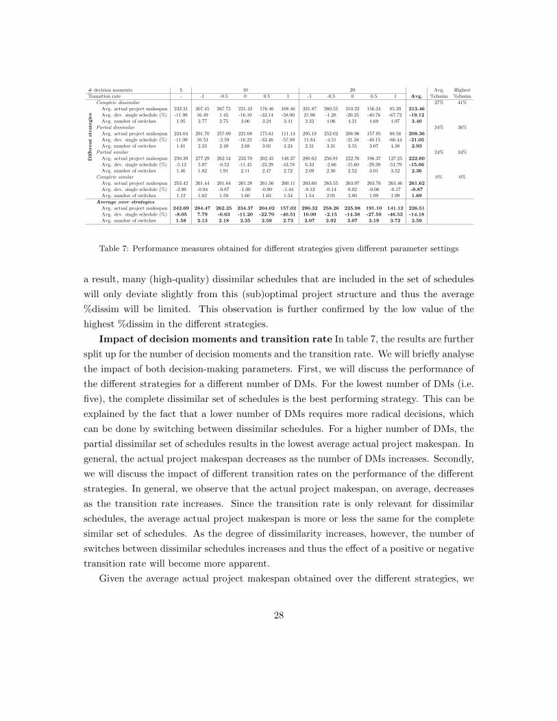
# decision moments 5 10 20 Avg. HighestTransition rate - -1 -0.5 0 0.5 1 -1 -0.5 0 0.5 1 Avg. %dissim %dissim

Diff

ere

nt

stra

tegie

s

Complete dissimilar 27% 41%Avg. actual project makespan 232.31 307.45 267.75 221.43 176.46 108.46 321.87 260.55 210.22 156.34 85.20 213.46Avg. dev. single schedule (%) -11.98 16.49 1.45 -16.10 -33.14 -58.90 21.96 -1.28 -20.35 -40.76 -67.72 -19.12Avg. number of switches 1.95 2.77 2.75 3.00 3.24 3.41 2.32 4.06 4.21 4.69 4.97 3.40

Partial dissimilar 24% 36%Avg. actual project makespan 234.64 291.70 257.09 221.08 175.61 111.14 295.18 252.02 206.96 157.95 88.56 208.36Avg. dev. single schedule (%) -11.09 10.53 -2.59 -16.23 -33.46 -57.89 11.84 -4.51 -21.58 -40.15 -66.44 -21.05Avg. number of switches 1.81 2.33 2.49 2.68 3.01 3.24 2.31 3.31 3.55 3.07 4.38 2.93

Partial similar 24% 34%Avg. actual project makespan 250.39 277.29 262.54 233.70 202.45 148.37 280.62 256.91 222.76 186.37 127.25 222.60Avg. dev. single schedule (%) -5.13 5.07 -0.52 -11.45 -23.29 -43.78 6.33 -2.66 -15.60 -29.39 -51.79 -15.66Avg. number of switches 1.46 1.82 1.91 2.11 2.47 2.72 2.09 2.30 2.52 3.01 3.52 2.36

Complete similar 0% 0%Avg. actual project makespan 253.42 261.44 261.64 261.28 261.56 260.11 263.60 263.55 263.97 263.76 263.46 261.62Avg. dev. single schedule (%) -3.98 -0.94 -0.87 -1.00 -0.90 -1.44 -0.12 -0.14 0.02 -0.06 -0.17 -0.87Avg. number of switches 1.12 1.62 1.59 1.60 1.63 1.54 1.54 2.01 2.00 1.99 1.99 1.69

Average over strategiesAvg. actual project makespan 242.69 284.47 262.25 234.37 204.02 157.02 290.32 258.26 225.98 191.10 141.12 226.51Avg. dev. single schedule (%) -8.05 7.79 -0.63 -11.20 -22.70 -40.51 10.00 -2.15 -14.38 -27.59 -46.53 -14.18Avg. number of switches 1.58 2.13 2.18 2.35 2.59 2.73 2.07 2.92 3.07 3.19 3.72 2.59

Table 7: Performance measures obtained for different strategies given different parameter settings

a result, many (high-quality) dissimilar schedules that are included in the set of schedules

will only deviate slightly from this (sub)optimal project structure and thus the average

%dissim will be limited. This observation is further confirmed by the low value of the

highest %dissim in the different strategies.

Impact of decision moments and transition rate In table 7, the results are further

split up for the number of decision moments and the transition rate. We will briefly analyse

the impact of both decision-making parameters. First, we will discuss the performance of

the different strategies for a different number of DMs. For the lowest number of DMs (i.e.

five), the complete dissimilar set of schedules is the best performing strategy. This can be

explained by the fact that a lower number of DMs requires more radical decisions, which

can be done by switching between dissimilar schedules. For a higher number of DMs, the

partial dissimilar set of schedules results in the lowest average actual project makespan. In

general, the actual project makespan decreases as the number of DMs increases. Secondly,

we will discuss the impact of different transition rates on the performance of the different

strategies. In general, we observe that the actual project makespan, on average, decreases

as the transition rate increases. Since the transition rate is only relevant for dissimilar

schedules, the average actual project makespan is more or less the same for the complete

similar set of schedules. As the degree of dissimilarity increases, however, the number of

switches between dissimilar schedules increases and thus the effect of a positive or negative

transition rate will become more apparent.

Given the average actual project makespan obtained over the different strategies, we

28

can determine at which transition rate the performance of an average set of schedules

is similar to a single schedule approach. In our experiment, this occurs at a transition

rate equal to around -0.63. This indicates that a set of schedules is beneficial compared

to a single schedule even when the former strategy requires redoing 63% of the work in

the current stage when alternative schedules are switched. Again, this shows that our

approach outperforms a single schedule approach. Furthermore, the different strategies

even outperform a single schedule approach when the number of DMs is lowest (i.e. equal

to 5) and thus the added value of the set of schedules is lowest.

Impact of uncertainty parameters In this section, we discuss the impact of the

uncertainty parameters in case that the partial dissimilar set of schedules (best strategy) is

used. Figure 8 shows the average actual project makespan on the primary axis, expressed

using a white bar in case that a set of schedules is used during project execution and a

grey bar to indicate the additional increase in project makespan in case that only a single

schedule is available. Also, the number of switches between alternative schedules is shown

on the secondary axis, expressed using a line chart. Figure 8a presents the results for

different parameter values of the types of uncertainty (i.e. low, medium and high), while

figure 8b shows the results for the different stages of uncertainty (early, uniform and late).

First of all, we aim to investigate the impact of uncertainty during project execution on

the project performance. Since the strategies developed in this research are used to cope

with the negative impact of disruptions, we will first analyse the average actual project

makespan in case that only a single schedule is available. We observe that the average

actual project makespan increases as the degree of uncertainty increases. Although the

difference in project makespan is rather limited for the low and medium cases, a higher

project makespan is observed for the high uncertainty case. Furthermore, the average

actual project makespan increases when the uncertainty mainly occurs in the later rather

than the earlier project stages. Secondly, we want to investigate the ability of the best

strategy to reduce the negative effect of uncertainty on the project performance for different

uncertainty scenarios. We observe that the average actual project makespan decreases when

the partial dissimilar set of schedules is used during project execution. The largest decrease

is reported in case that the uncertainty is high since the improvement potential is largest

in this scenario. With respect to the stages of uncertainty, we again observe that a slightly

higher average actual project makespan is obtained when the uncertainty mainly occurs

later in the project execution. In general, we note that the average number of switches

does not substantially differ between the various settings of the uncertainty parameters.

29

2.88

2.9

2.92

2.94

2.96

2.98

3

3.02

0

50

100

150

200

250

300

350

400

Low Medium High

Aver

age

num

ber

of sw

itche

s

Aver

age

actu

al p

roje

ct m

akes

pan

Degree of uncertainty

(a) Impact of the degree of uncertainty

2.88

2.89

2.9

2.91

2.92

2.93

2.94

2.95

2.96

150

170

190

210

230

250

270

290

310

Early Uniform Late

Aver

age

num

ber

of sw

itche

s

Aver

age

actu

al p

roje

ct m

akes

pan

Stage of uncertainty

(b) Impact of the stages of uncertainty

Figure 8: Impact of the different uncertainty scenarios

Problem features. Table 8 shows the overall performance of the different strategies given

various settings of the flexibility parameters (see section 0.5.1). We observe that the partial

dissimilar set of schedules results in the lowest average actual project makespan, indepen-

dent of the flexibility parameters. Also, the experiments indicate that the %flex has a

positive impact on the actual project makespan in an uncertain project environment. This

observation is intuitive since an increase in the number of alternatives results in a more

diverse set of back-up schedules. Consequently, the positive impact of the %flex is more ap-

parent for the complete (partial) dissimilar set of schedules than for the complete (partial)

similar set of schedules. Note that the actual project makespan obtained using a complete

similar set of schedules even increases as the %flex increases since the discrepancy between

a complete similar and dissimilar set of schedules becomes larger as more alternatives ex-

ist. We also observe that the average actual project makespan decreases as the %nested

increases. This implies that a lower actual project makespan can be obtained in the sit-

uation that alternatives are embedded in one another, which supports the claim that our

approach is especially interesting when more complex dependencies between alternatives

exist. Furthermore, the actual project makespan increases as the %linked increases mainly

due to the higher number of alternative activities that potentially should be scheduled in

case of a higher %linked. Finally, the experiments indicate that overall the lowest average

actual project makespan can be obtained with a uniform distribution of the alternatives

over the project horizon. Only a small increase in actual project makespan is observed in

case of an early or uniform flexibility distribution, while a deterioration in the performance

of the strategies is observed when the alternatives are positioned late in the project horizon.

We can conclude that it is preferred to diversify rather than concentrate alternatives in

30

%flex %nested0.25 0.5 0.75 1 0 0.25 0.5 0.75 1

Str

ate

gie

s Complete dissimilar 227.84 218.53 206.04 201.42 231.04 218.61 207.45 198.52 211.67Partial dissimilar 223.79 211.28 204.31 194.05 226.47 212.3 202.45 194.47 206.10Partial similar 234.17 222.84 220.97 212.44 237.88 230.89 214.04 213.64 212.57Complete similar 259.18 257.90 265.04 264.35 261.95 262.94 258.62 261.07 263.51

Flexibility distribution %linkedEarly Middle Late Uniform 0 0.25 0.5 0.75 1

Str

ate

gie

s Complete dissimilar 210.59 212.80 227.65 202.80 205.42 215.61 216.67 215.25 214.34Partial dissimilar 206.89 208.26 220.59 197.69 203.26 208.86 208.71 212.00 208.96Partial similar 219.63 223.06 233.74 213.99 220.69 221.21 223.77 223.41 223.94Complete similar 259.15 258.58 265.82 262.92 260.89 261.05 262.24 261.66 262.25

Table 8: Impact of the flexibility parameters on the actual project makespan

the project horizon. In case that a large number of alternatives should be concentrated in

the project horizon, it is better to focus on the early stages of the project since the effect

of switches is more limited in the later stages of the project.

0.6. Conclusions and future research

In the RCPSP-AS, multiple alternative ways to execute work packages exist in the

project structure and thus the problem consists of a selection and a scheduling subprob-

lem. In this research, we investigate the possibility to use the alternatives modelled in

the RCPSP-AS to support the baseline schedule in the face of uncertainty. Therefore, we

develop an approach for scheduling under uncertainty that is based on the construction of

a set of alternative schedules. More precisely, we present four strategies to construct such

a set of schedules varying from a complete similar to a complete dissimilar set of schedules.

These strategies can be distinguished based on the number of similar and dissimilar alter-

native schedules in the set of schedules. Since the aim of the procedure is to effectively and

efficiently protect the project execution against uncertainty, we monitor the performance of

the different strategies using two key performance measures: the actual project makespan

after disruptions (i.e. quality indicator) and the number of switches between alternative

schedules (i.e. effort indicator). The results show that a set of schedules outperforms a

single schedule scenario in the face of uncertainty, however, the performance of the solution

approach is impacted by the solution quality of the schedules. During the generation of

the set of schedules, two approaches are compared. The project execution can be initiated

with the schedule with the lowest baseline project makespan (i.e. reactive schedule) or the

lowest expected actual project makespan (i.e. proactive schedule) in the schedule set. We

observe that the proactive schedule requires less switches (i.e. lower effort), but results in

31

a slightly higher actual project makespan (i.e. lower quality). With respect to the different

strategies introduced in our research, we observe that the partial dissimilar set of schedules

performs best under various uncertainty scenarios, while the complete similar set of sched-

ules results in the highest actual project makespan. Furthermore, we analyse the impact

of the number of decision moments and the transition rate on the performance measures.

Finally, we investigate the impact of various uncertainty scenarios and problem parameters

of the RCPSP-AS.

The following research avenues could be investigated. In the current study, we model

the amount of work that needs to be redone when we switch from one alternative to

another using the transition rate. However, the concept of a transition rate could also

be used to model other economic aspects, such as the rework time, related to switching

alternatives. In case that we want to use the transition rate to express the cost of switching,

the problem becomes a multi-objective problem, which is an interesting extension of the

problem discussed in this research. Also, the robustness in the proposed solution approach

is obtained from combining high-quality back-up schedules with a low individual robustness.

One could improve the approach by increasing the robustness of the individual schedule in

the set of schedules. In general, our approach could be benchmarked with other proactive,

reactive and stochastic scheduling approaches as well as other strategies for the construction

of the set of schedules should be investigated. Finally, the computational results depend on

the topological structure of the project instances from the considered dataset As a result,

the design of the project instances could be validated and the performance of the proposed

approach could be tested on a realistic, industrial scale using a case study research.

Acknowledgement

We acknowledge the support provided by the Nationale Bank van Belgie (NBB) and the

Bijzonder Onderzoeksfonds (BOF) for the project, under contract number BOF12GOA021.

References

Aloulou, M. A., Portmann, M.-C., Vignier, A., 2002. Predictive-Reactive Scheduling for the Single Machine

Problem. In: Eighth International Workshop on Project Management and Scheduling - PMS 2002.

Valencia, Spain, pp. 39–42.

Artigues, C., Billaut, J.-C., Esswein, C., 2005. Maximization of solution flexibility for robust shop schedul-

ing. European Journal of Operational Research 165 (2), 314 – 328.

32

Artigues, C., Roubat, F., Billaut, J.-C., 1999. Characterization of a set of schedules in a resource-constrained

multi-project scheduling problem with multiple modes. International Journal of Industrial Engineering -

Theory, Applications and Practice 6, 112–122.

Billaut, J.-C., Roubellat, F., 1996a. Characterization of a set of schedules in a multiple resource context.

Journal of Decision Systems 5 (1-2), 95–109.

Billaut, J. C., Roubellat, F., 1996b. A new method for workshop real time scheduling. International Journal

of Production Research 34 (6), 1555–1579.

Briand, C., Despontin, E., Roubellat, F., 2002. Scheduling with time lags and preferences: a heuristic. In:

Eight International Workshop on Project Management and Scheduling - PMS 2002. Valencia, Spain.

Briand, C., La, H., Erschler, J., 2007. A robust approach for the single machine scheduling problem. Journal

of Scheduling 10, 209–221.

Capacho, L., Pastor, R., 2006. The ASALB Problem with Processing Alternatives Involving Different Tasks:

Definition, Formalization and Resolution. Springer Berlin Heidelberg, Berlin, Heidelberg, pp. 554–563.

Capacho, L., Pastor, R., Dolgui, A., Guschinskaya, O., 2009. An evaluation of constructive heuristic methods

for solving the alternative subgraphs assembly line balancing problem. Journal of Heuristics 15 (2), 109–

132.

Capek, R., Sucha, P., Hanzalek, Z., 2012. Production scheduling with alternative process plans. European

Journal of Operational Research 217 (2), 300 – 311.

Davenport, A. J., Gefflot, C., Beck, J. C., 2001. Slack-based techniques for robust schedules. In: Paper

presented at the constraints and uncertainty workshop, Seventh international conference on principles

and practice of constraint programming, 2001. Paphos, Cyprus.

Esswein, C., Billaut, J., 2002. Trade-off between flexibility and maximum completion time in the two-

machine flowshop scheduling problem. In: International symposium on combinatorial optimisation. Paris,

France.

Goa, H., 1995. Building robust schedules using temporal protection: an empirical study of constraint based

scheduling under machine failure uncertainty. Master’s thesis, Department of Industrial Engineering,

University of Toronto, Canada.

Herroelen, W., Leus, R., 2004. Robust and reactive project scheduling: a review and classification of

procedures. International Journal of Production Research 42 (8), 1599–1620.

Herroelen, W., Leus, R., 2005. Project scheduling under uncertainty: Survey and research potentials.

European Journal of Operational Research 165, 289–306.

Jensen, M., 2001. Robust and flexible scheduling with evolutionary computation. Ph.D. thesis, Department

of Computer Science, University of Aarhus, Denmark.

33

Kellenbrink, C., Helber, S., 2015. Scheduling resource-constrained projects with a flexible project structure.

European Journal of Operational Research 246 (2), 379 – 391.

Kis, T., 2003. Job-shop scheduling with processing alternatives. European Journal of Operational Research

151 (2), 307 – 332.

Kosztyan, Z. T., 2015. Exact algorithm for matrix-based project planning problems. Expert Systems with

Applications 42 (9), 4460 – 4473.

Kuster, J., Jannach, D., Friedrich, G., 2008. Extending the RCPSP for modeling and solving disruption

management problems. Applied Intelligence 31 (3), 234.

Lambrechts, O., Demeulemeester, E., Herroelen, W., 2008. Proactive and reactive strategies for resource-

constrained project scheduling with uncertain resource availabilities. Journal of Scheduling 11 (2), 121–

136.

Marle, F., Vidal, L.-A., 2016. Managing Complex, High Risk Projects: A Guide to Basic and Advanced

Project Management. Springer-Verlag London.

Mauguire, P., Billaut, J.-C., Artigues, C., 2002. Grouping jobs on a single machine with heads and tails to

represent a family of dominant schedules. In: Eighth International Workshop on Project Management

and Scheduling - PMS 2002. Valencia, Spain.

Servranckx, T., Vanhoucke, M., 2019. A tabu search procedure for the resource-constrained project schedul-

ing problem with alternative subgraphs. European Journal of Operational Research 273 (3), 841 – 860.

Sevaux, M., Sorensen, K., 2004. A genetic algorithm for robust schedules in a one-machine environment

with ready times and due date. 4OR 2, 129–147.

Tao, S., Dong, Z. S., 2018. Multi-mode resource-constrained project scheduling problem with alternative

project structures. Computers & Industrial Engineering 125, 333 – 347.

Tao, S., Wu, C., Sheng, Z., Wang, X., 2018. Stochastic project scheduling with hierarchical alternatives.

Applied Mathematical Modelling 58, 181 – 202.

Tavares, L., Ferreira, J., Coelho, J., 1998. On the optimal management of project risk. European Journal

of Operational Research 107, 451–469.

Van de Vonder, S., Ballestın, F., Demeulemeester, E., Herroelen, W., 2007. Heuristic procedures for reactive

project scheduling. Computers & Industrial Engineering 52 (1), 11 – 28.

Van de Vonder, S., Demeulemeester, E., Herroelen, W., 2005. Heuristic Procedures for Generating Stable

Project Baseline Schedules. Katholieke Universiteit Leuven, Faculty of Economics and Applied Eco-

nomics, Department of Applied Economics.

34

Van de Vonder, S., Demeulemeester, E., Herroelen, W., 2008. Proactive heuristic procedures for robust

project scheduling: An experimental analysis. European Journal of Operational Research 189 (3), 723 –

733.

Van de Vonder, S., Demeulemeester, E., Herroelen, W., Leus, R., 2006. The trade-off between stability

and makespan in resource-constrained project scheduling. International Journal of Production Research

44 (2), 215–236.

Vanhoucke, M., Coelho, J., 2016. An approach using SAT solvers for the RCPSP with logical constraints.

European Journal of Operational Research 249 (2), 577 – 591.

Vidal, L.-A., Marle, F., Bocquet, J.-C., 2011. Using a delphi process and the analytic hierarchy process

(AHP) to evaluate the complexity of projects. Expert Systems with Applications 38 (5), 5388 – 5405.

Weglarz, J., Jozefowska, J., Mika, M., Waligora, G., 2011. Project scheduling with finite or infinite number

of activity processing modes - a survey. European Journal of Operational Research 208, 177–205.

Wiers, V., 1997. A review of the applicability of OR and AI scheduling techniques in practice. Omega

25 (2), 145 – 153.

Wu, S. D., Byeon, E.-S., Storer, R. H., 1999. A graph-theoretic decomposition of the job shop scheduling

problem to achieve scheduling robustness. Operations Research 47 (1), 113–124.

35