Strategic Trading, Welfare and Prices with Futures Contracts1

Hugues Dastarac2

October 2021, WP #841

ABSTRACT

Derivatives contracts are designed to improve risk sharing in financial markets, but among them, forwards, futures and swaps often appear redundant with their underlying assets: buying the asset and storing it is equivalent to buying it later. I show that imperfect competition in a dynamic market creates an incompleteness, opening gains from trading futures; but surprisingly, in equilibrium, agents trading these contracts have lower welfare than without futures. To mitigate their price impact, buyers (sellers) of an asset postpone profitable trades, exposing themselves to upward (downward) future spot price movements: buyers (sellers) would like to buy (sell) futures. However, when futures are introduced, traders also want to influence the spot price at futures maturity to increase futures payoff: this leads buyers (sellers) to sell (buy) futures. Moreover, despite the absence of market segmentation that would preclude arbitrage, the futures price can be above or below the spot price.

Keywords: Futures, Imperfect Competition, Inefficiency, Mispricing.

JEL classification: G10, G13, G15

1 I am very grateful to Bruno Biais, Sabrina Buti, Jérôme Dugast, Stéphane Guibaud, Florian Heider

(discussant), Johan Hombert, Marzena Rostek and Liyan Yang (discussant) for very helpful discussions and comments, and audiences at Banque de France, NISM Capital Market Conference and SAFE Market Microstructure Conference. All errors are mine. The views expressed here are those of the author and do not necessarily reflect those of Banque de France. 2 Banque de France, hugues.dastarac@banque-france.fr

Working Papers reflect the opinions of the authors and do not necessarily express the views of the Banque de France. This document is available on publications.banque-france.fr/en

Banque de France WP #841 ii

NON-TECHNICAL SUMMARY

Forward and futures contracts are pervasive in security, currency and commodity markets. These derivative contracts allow traders to buy or sell an underlying asset at a future date at a pre-agreed price: when the future asset price is not predictable, this hedges traders against adverse price movements for future transactions. Swaps are portfolios of futures of different maturities. Futures are often used by agents who cannot trade today: for instance, a wheat producer wishes to hedge against uncertainty regarding the price at which it will sell its crop before sowing, an international company wishes to hedge against exchange rate risk regarding future income or expenses, etc. Were it possible, agents could as well buy or sell their asset immediately, and they would be perfectly hedged without resorting to futures. But there are important cases, notably major sovereign bond markets, where futures are traded while agents plausibly can trade the asset immediately. For instance, in safe government bond markets (US, Germany, France, …), it is possible to trade with relatively limited constraints: it is possible to borrow funds to purchase a bond by putting it as collateral for the lender; many maturities are available to investors having such a preference without having to wait for issuance; and spot markets can absorb very large quantities. Yet futures are massively traded: in the US, there have always been between 1.5 and 2 trillion dollars of Treasury futures outstanding over the last three years. One partial explanation is that some investors exploit the spread between futures price and spot prices: but this does not explain why futures are traded in the first place. Therefore, if it is easy to buy or sell a sovereign bond immediately, why should investors use futures contracts? Is their introduction desirable? This paper provides a theoretical explanation for this, and finds in particular that 1) futures contracts decreases traders’ overall profitability, and 2) futures and their underlying asset trade at different prices, although no investor is precluded to trade in either market. A first result is that a market incompleteness, i.e. a situation where traders would like to trade derivatives, is created by imperfect competition. When traders are imperfectly competitive, i.e. when they care about the impact of their trades on equilibrium prices, they choose to slice the quantities they want to buy or sell into smaller pieces to be executed successively. This behavior is widely observed in practice. By delaying trade in this way, traders also expose themselves to the risk that the price moves when they trade later: buyers would then fear that the price moves up, and sellers that the price moves down. If futures were introduced, buyers of the underlying asset may be willing to buy futures to sellers of the underlying asset: this rationalizes the use of futures in markets like for safe sovereign bonds. But when futures are introduced, they are not traded in order to share risk. Traders instead trade futures in a direction opposite to their hedging needs: this is because they also want to influence the futures’ payoff, which is the difference between the spot price at futures’ maturity, and the futures price at which the contract was set. To do so, they modify their trading strategy in the underlying asset in order to influence the spot price at futures’ maturity. Since futures are not used for risk sharing, they may not smooth traders’ revenue and therefore adversely impact their risk-adjusted profitability: I show this formally. However,

Banque de France WP #841 ii

this does not necessarily call for further regulation by financial market authorities. In fact, traders in this model are assumed to be large, and all are adversely affected, so that they may devise rules by themselves, e.g. within the framework of the futures exchange.

Finally, I show that the futures contract can trade below or above the underlying asset, without assuming storage cost or non-zero interest rates. This is surprising, because an investor could then purchase the cheapest asset (underlying or futures contract) and simultaneously sell the most expensive, locking in a risk-free profit while making both prices converge. Such failures of the law of one price are almost always justified by the fact that some traders are constrained not to trade in one market or the other, and limited capacity by those who can trade in both markets to exploit the difference. For instance, in Keynes’ theory of normal backwardation, speculators buy futures to commodity producers and cannot trade in the spot market. But some contemporary commodity traders explicitly refer to simultaneous trade in the spot and futures market as a source of profit. While trading constraints may certainly explain part of observed spreads, imperfect competition in markets with large traders may well be another valid explanation, as this model suggests.

Trading stratégique, profitabilité et prix dans les marchés de contrats à terme

RÉSUMÉ

Les produits dérivés sont conçus pour améliorer le partage du risque au sein des marchés financiers. Toutefois, parmi ceux-là, les contrats à terme de type forward, futures et swap apparaissent redondant avec l’actif sous-jacent : acheter l’actif et le stocker est équivalent à l’acheter à terme. Nous montrons que la concurrence imparfaite dans un marché dynamique crée une incomplétude de marché, ouvrant des gains à l’échange de contrats à terme ; mais de façon surprenante, à l’équilibre, les agents qui échangent ces contrats ont une rentabilité moindre par rapport au cas où ces contrats ne sont pas disponibles. Pour atténuer leur impact sur les prix, les acheteurs (vendeurs) d’un actif retardent une partie de leurs transactions, ce qui les expose à une hausse (baisse) du prix futur : les acheteurs (vendeurs) souhaiteraient donc acheter (vendre) des contrats à terme. Mais lorsque ces contrats sont introduits, les agents souhaitent aussi influencer le prix spot au terme du contrat pour en accroître le rendement : ce qui conduit les acheteurs (vendeurs) à vendre (acheter) le contrat à terme. De plus, en dépit de l’absence de segmentation du marché qui empêcherait l’arbitrage, le prix du contrat à terme peut être au-dessus ou en-dessous du prix spot contemporain.

Mots-clés : Contrats à terme, concurrence imparfaite, inefficacité, aberrations de prix

Les Documents de travail reflètent les idées personnelles de leurs auteurs et n'expriment pas nécessairement la position de la Banque de France. Ils sont disponibles sur publications.banque-france.fr

iii iii

1 Introduction

Forward and futures contracts are pervasive in fixed income, stock, commodities

and currency markets. These derivative contracts allow traders to buy or sell an

underlying asset at a future date at a pre-agreed price:1 when the asset price in the

future is uncertain, they hedge traders against adverse price movements for future

transactions. This hedging demand often comes from an inability to trade the asset

directly today: the asset may be a commodity that is not yet produced, short-selling

the asset or borrowing funds to purchase the asset may be di�cult.2

But there are important examples where futures are massively traded even if

the asset can be easily traded today. For instance, US Treasury bonds markets

are very liquid, and traders easily borrow funds to buy a bond by putting the

bond as collateral, so that few of them should be constrained. Yet the outstanding

amount (“open interest”) of Treasury futures peaked above $2,000bn in February

2020 (CFTC), and was about $1,600bn in early May 2021. These numbers have

been related to arbitrage between Treasury bonds and Treasury futures (Barth and

Kahn 2021).3 While arbitrage for sure explains part of the high open interests

mentioned above, it does not explain why futures are traded in the first place, if

trading is relatively unconstrained. In addition, arbitrage opportunities, usually

explained with constraints that prevent traders to act in both markets, in this case

deserve additional explanation.

Another concern with futures is that some traders want to manipulate, as evi-

denced by numerous cases throughout history:4 as the futures payo↵ is the di↵er-

ence between the underlying asset price tomorrow and the pre-agreed futures price,

a trader holding futures may be tempted to trade the underlying asset to raise the

underlying price tomorrow.5

Why do traders trade forwards and futures when constraints to trade on the spot

1Forward contracts are traded over-the-counter, futures are listed. In this paper, I make nodi↵erence between the two types of contracts.

2see Stoll (1979), Hirshleifer (1990), Froot et al. (1993), Raab and Schwager (1993), Routledgeet al. (2000) among others.

3For instance, if the former are cheaper than the latter, it is profitable to buy the Treasury bondand enter a short position in the associated futures, then hold the positions until futures maturity.As variations in Treasury bonds prices are o↵set by an opposite futures payo↵, this strategy wouldbe riskless without constraints on arbitrageurs.

4In the US, the Commodity Exchange Act of 1936 already forbade futures manipulation. Pub-lic disclosure of traders’ position concentration has been done since 1927 by the CFTC and itspredecessors, which aims at limiting manipulation. More recently, LIBOR manipulation by banktraders benefited banks’ futures positions.

5Kumar and Seppi (1992), Pirrong (1993), Jarrow (1994).

2

market are light? How do arbitrage opportunities emerge without such constraints?

What is the e↵ect of futures on traders’ welfare?

To answer these questions, in this paper I provide a dynamic trading model where

the only friction is imperfect competition. Traders care about the price impact of

their trades, implying that without futures, they choose to defer some profitable

trades to tomorrow, and thus to be exposed to asset price risk tomorrow: buyers

fear price increases, sellers fear price increases, an incompleteness that futures would

solve. But when futures are introduced, traders also want to influence futures payo↵

by trading the underlying asset at maturity to increase their payo↵ from the futures.

In equilibrium, traders choose negative hedge ratios: sellers of the underlying asset

buy the futures to buyers of the underlying asset. But both buyers and sellers

attempt to influence prices in opposite directions, and prices remain unchanged.

Futures are less traded if the price volatility increases. Overall, futures decrease

all traders’ welfare unless futures payo↵ influence is impeded. In addition, futures

and the underlying asset trade at di↵erent prices (whether or not payo↵ influence

is impeded), although markets are not segmented. I also show that sellers of the

underlying asset have greater welfare than buyers when the futures price is higher

than the spot price, suggesting that traders in this model trade in the opposite

direction to arbitrageurs: my model thus gives an account of deviations from the

law of one price in the absence of constraints.

I study a model in which risk averse traders can trade a risky asset at two dates

0 and 1. All information is symmetric. Traders di↵er by their initial inventories of

the asset, and have identical preferences. At each trading date, traders meet in a

centralized market. At date 1, some exogenous customers post an inelastic quantity

that is unknown at date 0 and independent from the asset payo↵. Date 1 price is

low when customers sell, and vice versa. Imperfect competition means that traders

care about the impact of their trades on equilibrium prices.

I first study the equilibrium without futures: this allows to isolate a hedging

demand for futures contracts, on top of being a natural benchmark. At date 0,

trades a↵ect both date 0 and date-1 prices, and that there is a trade-o↵ between

the two. To see it, consider a seller of the asset. Given other traders’ strategies,

if they sell more of the asset at date 0, the date-0 price decreases more, which is

costly to them, but they arrive at date 1 with less inventory, which makes date-1

price decrease less. Balancing the two impacts, sellers optimally chose to defer some

trades to date 1. Buyers make the same reasoning to limit upward price pressure. In

equilibrium neither sellers nor buyers succeed in moving prices. When competition

3

increases, traders delay less trade as their impacts on prices are diluted.

A second observation is that the liquidity shock moves date-1 price and thus

a↵ects the terms of trade between buyers and sellers. Buyers face the risk of a

higher date-1 price than expected, and seller face the risk of lower price. The cost

associated with this risk may exceed the price impact benefit of delaying trade.

Hence with higher uncertainty on the liquidity shock, traders trade more at date 0.

These two observations shed light on the incompleteness that futures contracts

solve: by selling a futures contract, a seller of the underlying asset would hedge

against downward date-1 price movements and thus is more willing to postpone

trade. Symmetrically, buyers of the underlying are willing to buy futures.

Then I introduce futures contracts, maturing at date 1: these contracts pay o↵

the di↵erence between date-1 price and the futures price, the latter being determined

in equilibrium at date 0. With futures, the incentive to a↵ect date-1 price completely

changes: on top of mitigating the overall price impact of inventory liquidation, buyers

of the future want to push the date-1 price up, and sellers of the futures want to pull

it down. This would be achieved by trading the asset at date 1 in the appropriate

direction. This incentive has long been fought by public authorities.6

I first observe that the incentive to influence the date-1 spot price is so strong

that when date-1 price volatility is low, traders’ welfare function is not concave

anymore: traders would like to buy an arbitrarily large amount of the underlying

asset, and to sell an even higher amount of futures in order to re-sell the asset at date

1. This would push date-1 price down and increase the payo↵ of the short futures’

position. The opposite is also possible: to sell spot and to buy futures at date 0. To

find an equilibrium, I have to assume that price volatility is high enough.7

When an equilibrium exists, the incentive to influence the spot price indeed

dominates the hedging motive for trading futures, and traders choose negative hedge

ratios: sellers of the underlying asset buy futures, instead of selling futures if they

traded for hedging, and buyers of the underlying sell futures. But traders fail to

influence the spot price in equilibrium: both buyers and sellers push the price in

their preferred directions, and the forces balance so that equilibrium prices are not

a↵ected. In addition, buyers and sellers trade more quickly the underlying asset:

sellers want to sell less at date 1, buyers to buy less, in order not to push the

6The Commodity Exchange Act, passed in the US in 1936, forbids manipulation in futuresmarket. For theory, see Kumar and Seppi (1992), Pirrong (1993) among many others.

7In practice, financing constraints would limit the quantities traded in the asset and futures.

4

price in a direction that would decrease futures’ payo↵. I also show that imperfect

competition is an essential ingredient to having futures in this environment: as

the number of traders becomes arbitrarily large, traders delay less trades and the

quantity of futures shrinks to zero.

Regarding traders’ welfare, there are two opposite forces: the acceleration of

trading in the underlying asset brings a welfare gain. But trading futures in a way

contrary to a hedging strategy entails more risk and a welfare loss. I show that

traders’ welfare is lower with futures than without, because of traders’ attempts to

influence futures’ payo↵.8,9

I also show that futures trade at a spread (“basis”) with the underlying asset in

equilibrium, that is proportional to expectation of the date 1 supply shock. This

basis can go in either direction, as observed in practice. The basis does not emerge

because of trading constraints, as is the case in many other models. It emerges

because the futures price and the spot price are sensitive to the expectation of the

supply shock through di↵erent channels, and with a higher sensitivity for the futures

price: the futures price reflects an expectation of the date 1 price, and the spot price

reflects traders’ sensitivity to the surplus of date 1 transaction.

While the existence of a basis would not be surprising in a setting with investors

constrained not to trade in one market or the other, it is more so in this setting

with no constraint: it seems that traders may profitably benefit from this spread by

buying spot and selling the futures if the spot price is below the futures price and

vice-versa. In fact, I show that traders are better o↵ when they trade against the

basis, selling cheap and buying expensive. Since the futures price decreases more

with the expectation of the supply shock than the spot price, a futures price above

the spot reflects a high spot price, thus improved terms of trade in the underlying

asset for sellers. Therefore, my model provides a new source of arbitrage opportu-

nities, compared to settings where some traders have limited capacity to enter the

spot or the futures market.

8I also show in the online appendix that with contracts whose payo↵ cannot be influenced,futures contracts would indeed raise welfare: thus in the setting of this paper, futures decreasewelfare because each party seeks to influence futures payo↵.

9Such a situation is reminiscent of signal-jamming models a la Fudenberg and Tirole (1986)and Stein (1989), but in these models, the mechanism is di↵erent: crucial is the inability of aprincipal to observe the unobservability of a strategic agent’s action by a principal. The principalcorrectly anticipates manipulation, but the agent always manipulates because if no manipulationwas expected by the principal, he/she would profitably manipulate. In my model, all informationis symmetric. Recently, Yang and Zhu (2021) have applied this idea to large traders trying tomanipulate the central bank’s beliefs about the economy’s fundamental to force intervention.

5

Literature review. Many papers study how derivatives arise in the presence of

various constraints, in contrast to the present paper. A first strand studies hedg-

ing demand when traders face financing constraints: Froot et al. (1993) show how

derivatives emerge when it is costly for a firm to raise external funds. Raab and

Schwager (1993) show that futures can be used to complete the market when there

are short-selling restrictions. Goldstein et al. (2013) provide a model in which some

traders end up with negative hedge ratios, as in the present paper. The mechanism

is very di↵erent, as it relies on information acquisition and market segmentation.

A substantial literature on futures trading in commodities markets also studies the

role of constraints on traders. First, in the theory of storage10 the market as a whole

cannot short the commodity beyond existing stocks. Routledge et al. (2000) study

its implications for futures pricing. This constraint is absent from my model. Sec-

ond, in the theory of normal backwardation (Keynes 1930, Hicks 1940, Hirshleifer

1990), producers are willing to o✏oad the price risk of their future production to

risk averse speculators who cannot trade in the spot market. Thus, in these models,

traders cannot trade in the spot market together with futures markets. Gorton et al.

(2012) put the theories of storage and normal backwardation into a single model and

link them to inventories.

A large literature make derivatives emerge because of di↵erent traders’ pref-

erences. Oehmke and Zawadowski (2015, 2016) show that when swaps have ex-

ogenously low transaction costs, the natural holder of derivatives are those with

short-term horizon, while long term investors hold the underlying. In my model

transaction costs are endogenously low, because forwards have a shorter maturity

than the underlying. In Biais et al. (2016) and Biais et al. (2019), some traders are

specialized in managing an asset and seek to o✏oad the risk of this asset through

a derivative contract. In Biais et al. (2019) di↵erences in preferences imply that

derivatives are needed to implement optimal risk sharing.

The closest paper to mine is Rostek and Yoon (2021), in which the authors

show that under imperfect competition and without exogenous market segmentation,

non-redundant derivative products endogenously emerge, with an impact welfare

that can be positive or negative. The mechanisms are very di↵erent however: in

10Kaldor (1939), Williams and Wright (1991), Deaton and Laroque (1992, 1996). Williams andWright (1991) notice that futures and spot markets are redundant, which is not the case in mymodel.

6

Rostek and Yoon (2021), the crucial ingredient is that traders have limited ability

to condition demand in one asset on prices of other assets. Derivative products are

built as portfolios of, and have the same maturity as the underlying assets (e.g. like

CDS), and can generally increase or decrease welfare. In the present paper, traders

can condition their demand schedule in one asset on other asset prices, and non-

redundant futures arise because they have shorter maturity than the underlying; the

unambiguously negative welfare e↵ect arises because futures’ payo↵ depends on the

underlying spot price (like options, but unlike CDSs).

The present paper connects to the literature on dynamic trading with imperfectly

competitive double auctions. Vayanos (1999), Du and Zhu (2017) and Rostek and

Weretka (2015) study dynamic trading strategies without forward contracts. Du�e

and Zhu (2017) and Antill and Du�e (2018) explore the ability of size discovery

mechanisms to overcome the ine�ciency. This paper is to my knowledge the first to

make forward/futures contracts emerge in this context.

Derivatives manipulation when traders try to influcence the underlying spot price

has also triggered extensive research (Easterbrook 1986, Kumar and Seppi 1992,

Pirrong 1993, Jarrow 1994, among others). In these papers, one player has market

power with respect to competitive traders. I study a more general equilibrium where

all traders seek to influence the spot price, and to counter influence from traders on

the opposite side.

The paper is organized as follows. Section 2 presents the setting. Section 3 solves

the imperfect competition equilibrium without forward contracts, and derives the

result that uncertainty on the supply shock accelerates trading. Section 4 highlights

the gains from trading the risk on the supply shock. Section 5 introduces forward

contracts and solves for the equilibrium. Section 6 gives trader welfare with and

without derivatives, and compares them. Section 7 focuses on the spread between

spot and futures prices. Section 8 concludes.

2 Setting

There are three dates t = 0, 1, 2. There is one risky asset that pays o↵ at t = 2

an ex ante unknown amount

v = v0 + ✏1 + ✏2

7

per unit, where ✏1 and ✏2 are independent and normally distributed with mean 0 and

respective variances �21 and �2

2.11 At date 1, ✏1 is released before any action takes

place. All information about ✏1 or ✏2 is symmetric. It is also possible to borrow and

save cash at the risk-free rate normalized to zero.

There are two types of traders. Buyers all start with initial inventory Ib,0 of

the risky asset at date 0, and sellers all start with inventory Is,0 > Ib,0. There are

B buyers, and S sellers, with the requirement that N = B + S � 3.12 I denote

I0 = SN Is,0 +

BN Ib,0 the average trader inventory. Inventories are publicly known

before the date 0 market opens.

Traders maximize the expected utility of their terminal wealth. Their utility is

negative exponential (CARA), with risk aversion parameter � for both types. Thus

gains from trade arise from inventory di↵erences. Traders are forward-looking and

fully rational: in particular, they perfectly anticipate at t = 0 the date-1 equilibrium

and adjust their actions accordingly.

At date 0, traders meet in a centralized market where they simultaneously trade

the risky asset and enter futures contracts. Futures contracts pay o↵

vf = p1 � f0, (2.1)

where p1 is the asset price at date 1 and f0 is the futures price at date 0, both to be

determined in equilibrium.13 For simplicity, I ignore margin constraints associated

with futures.

Markets operate through uniform-price double auctions, as in Kyle (1989). Traders

of type k = b, s simultaneously post demand schedules qk,0(p0, f0) for the risky asset

and xk(p0, f0) for the futures contract, conditional on date 0 information. All traders

of type k purchase the same equilibrium quantity qk,0 of the underlying asset and en-

11The normality assumption is for analytical tractability. It implies that the payo↵ can benegative without lower bound, which is not consistent with real world limited liability: one coulduse truncated normal distributions instead. However, at least for date 1 trade and for smallprobabilities of negative v lead to results approximately identical with and without lower truncationof the probability distribution.

12The condition N � 3 ensure existence of equilibria in linear strategies. When there are onlytwo traders, Du and Zhu (2017) show existence of equilibria in non-linear strategies.

13Defining futures in this way suggests settlement is financial rather than physical. Physicalsettlement means that a trader with a short position in the futures contract deliver the underlyingasset at maturity. Financial settlement means that a trader with a short futures position paysthe di↵erence between the underlying asset price at futures maturity and the futures price whenthe position was initiated. In practice financial settlement is quite common, even with contractslabelled “physically settled” or “deliverable”, like metal futures on the London Metal Exchange orthe COMEX are hybrid: exchange rulebooks indicate that settlement occurs either by delivery orfinancially by o↵setting a contract with an opposite contract at maturity.

8

ter the same position xk in the futures contract.14 A walrasian auctioneer computes

the equilibrium prices p⇤0 and f ⇤0 that clear the asset and futures markets. Futures

are in zero-net supply, and traders do not have pre-existing futures positions. Thus

the market clearing conditions at date 0 are

Bqb,0 + Sqs,0 = 0, (2.2)

Bxb + Sxs = 0. (2.3)

Traders of type k arrive in the date-1 market with inventory Ik,1 = Ik,0 + qk,0.

At date 1, the market for the risky asset re-opens and there is a liquidity shock

Q. The signing convention is that when Q > 0, some unmodelled traders are willing

to sell the asset to traders of type b and s. Conditional on date 0 information,

Q is normally distributed with mean E0[Q] and variance �2Q. In the model I will

use mostly the variance of Q/N , which is �2q = �2

Q/N2. The constant N2 is a

convenient normalization. I also assume that Q is jointly normally distributed with,

and independent from ✏1 and ✏2: this means that Q is a pure liquidity shock. The

date-1 market again operates through a uniform-price double auction. Traders of

type k post the same demand schedule qk,1(p1). In equilibrium, they purchase a

quantity qk,1 of the asset that satisfies the market clearing condition:

Bqb,1 + Sqs,1 = Q. (2.4)

(2.4) pins down the equilibrium price p⇤1, and thus the futures payo↵. The terminal

wealth of a trader of type k is thus

Wk = Ik,0v + qk,0(v � p0) + qk,1(v � p1) + xk(p1 � f0). (2.5)

I look for subgame-perfect Nash equilibria in demand schedules, with symmetric

strategies for all traders of a given type. The conditions for equilibrium are de-

scribed in definitions 1, 2 and 5. Specifically, I look for equilibria where demand

schedules are linear, as in most of the literature in a CARA-normal framework.15

In these equilibria, demand schedules are not constrained to be linear, but a lin-

ear demand schedule by trader k is the best response to linear demand schedules

by other traders.16 As there is neither information asymmetry nor uncertainty on

14When traders are strategic, such equilibria exist and are a natural focus of analysis. I furtherspecify the equilibrium concept when traders are strategic in Sections 3 and 5.

15Cf. Kyle (1989), Vayanos (1999), Malamud and Rostek (2017) among many others.16To the best of my knowledge, the existence of equilibria in nonlinear demand schedules with

9

supply shocks when traders post their demand schedules, an equilibrium multiplic-

ity problem arises (Klemperer and Meyer 1989). I use the trembling-hand stability

criterion to select a unique equilibrium (see Vayanos 1999).17

3 Equilibrium without futures

In this section I study the benchmark case where traders are non-competitive and

there are no futures, constraining xk = 0.18 The setting is similar to Vayanos (1999)

and Rostek and Weretka (2015). This allows to emphasize the intertemporal trade-

o↵ that traders face at date 0, which the presence of futures a↵ects. In equilibrium,

as buyers and sellers follow symmetric strategies, equilibrium prices are not a↵ected.

Yet quantities traded are reduced relative to the competitive benchmark.

The intertemporal trade-o↵ that traders face at date 0 is based on foresight of

the date-1 equilibrium, given traders’ inventories after date 0 trade. Thus Section

3.1 studies the date-1 equilibrium, which also allows to show how traders manage the

impact of their trades on contemporaneous price. Then I present the intertemporal

trade-o↵ in Section 3.2.

3.1 Date 1 equilibrium: static price impact management

At date 1, trader k maximizes the certainty equivalent of (2.5), which is well

known to be the mean-variance criterion given the normal distribution of ✏2:

cWk,1 = Ik,0v1 + qk,0(v1 � p0) + qk,1(v1 � p1)���2

2

2(Ik,1 + qk,1)

2, (3.1)

where v1 = v0 + ✏1 is the expected payo↵ v conditional on date 1 information.

Traders take the impact of their demand on the equilibrium price into account,

taking the residual demand curve, which is the sum of all other traders’ demand

three traders or more and normally distributed payo↵s has not been proven. Equilibria in non-linear strategies have been studied with only two traders and normally distributed payo↵s (Du andZhu 2017), or with three traders but payo↵s not normally distributed (Glebkin et al. 2020).

17An alternative approach, in the spirit of Klemperer and Meyer (1989), would assume thattraders face supply shocks Q0 at date 0 and Q1 ⌘ Q at date 1 that are revealed after traders haveposted their demand schedules. Thus it would require introducing an additional supply shock Q0,which would complicate notations without additional insight.

18In appendix A, I solve the competitive equilibrium where traders do not manage the priceimpact of their trades. Traders realize all gains from trade at date 0: they arrive at date 1 withequal inventories, which is the Pareto allocation. This is because they do not care about the priceimpact of their trades.

10

curves, as given. For a given quantity qk,1 demanded by a trader of type k, this

residual demand curve implies an equilibrium price p1, and a marginal increase in

the quantity demanded by this trader of type k implies a marginal price impact

@p1/@qk,1. Di↵erentiating the certainty equivalent of wealth (3.1), the first order

condition for a trader of type k is

v1 � p1 � qk,1@p1@qk,1

= ��22(Ik,1 + qk,1).

I look for equilibria in linear strategies: a trader of type k expects to face a linear

residual demand curve, and I denote its constant slope by 1/�k,1, so that @p1/@qk,1 =

�k,1. Thus trader k’s optimal demand schedule given this residual demand schedule

is

q⇤k,1(p1,�k,1) =v1 � p1

�k,1 + ��22

� ��22

�k,1 + ��22

Ik,1. (3.2)

As all traders follow linear strategies given a linear residual demand curve, summing

optimal demand (3.2) over other traders, the residual demand curve that a trader

faces has slope

B ⇥ (�b,1 + ��22)

�1 + (S � 1)⇥ (�s,1 + ��22)

�1 for a seller,

(B � 1)⇥ (�b,1 + ��22)

�1 + S ⇥ (�s,1 + ��22)

�1 for a buyer.

Requiring consistency of slopes of the residual demand curve faced by all traders

with actual equilibrium schedules leads to the following system of equations:

8<

:�s,1 = (B(�b,1 + ��2

2)�1 + (S � 1)(�s,1 + ��2

2)�1)�1

�b,1 = ((B � 1)(�b,1 + ��22)

�1 + S(�s,1 + ��22)

�1)�1. (3.3)

I can now formally define the equilibrium of the date 1 market.

Definition 1. Demand schedules qnk,1(p1) for k = b, s and a price pn1 is a date-1

equilibrium if:

• demand schedules qnk,1(p1) maximize (3.1), given price impact �k,1, i.e. satisfy

(3.2);

• price impacts �k,1 satisfy (3.3);

• the market clearing condition (2.4) holds.

11

The system of equations (3.3) is easily solved, which leads to the following propo-

sition.

Proposition 1 (Vayanos (1999), Malamud and Rostek (2017)). A date-1 equilib-

rium in linear strategies with imperfect competition exists and is unique. In this

equilibrium,

�s,1 = �b,1 =��2

2

N � 2,

so that equilibrium demand schedules are:

qnk,1(p1) =N � 2

N � 1

v1 � p1��2

2

� Ik,1

�. (3.4)

The equilibrium quantities traded by buyers and sellers are

qnb,1 =N � 2

N � 1

S

N(Is,1 � Ib,1) +

Q

Nand qns,1 =

N � 2

N � 1

B

N(Ib,1 � Is,1) +

Q

N. (3.5)

The equilibrium price is

pn1 = v1 � ��22

✓I1 +

N � 1

N � 2

Q

N

◆, (3.6)

where I1 = S/NIns,1 + B/NInb,1 is the date 1 average inventory across traders before

date 1 trade.

The quantity traded by trader of type k is reduced by a factor (N � 2)/(N � 1)

with respect to the competitive equilibrium, as shown in equation (3.5). This results

in imperfect risk sharing: traders of type k end up with

Ik,1 + qnk,1 =N � 2

N � 1I1 +

1

N � 1Ik,1 +

Q

N, (3.7)

and thus retains a fraction 1/(N � 1) of her initial inventory Ik,1. In the perfect

competition benchmark, all traders would end up with equal inventories.

The quantity traded at date 1 by each class of traders depends on date-0 equi-

librium trade, since Ik,1 = Ik,0 + qk,0. I fully solve the equilibrium date-1 trade in

Section 3.2.

The equilibrium price equals the underlying asset expected payo↵ conditional on

information available at date 1, minus an inventory risk premium which is the risk

aversion � times asset variance �22, times inventories. The factor (N�1)/(N�2) > 1

in front of the liquidity shock Q an reflects imperfect competition markup charged

12

by traders to provide liquidity.

3.2 Date 0: dynamic and static price impact management

I now analyze the intertemporal trade-o↵ regarding price impact at date 0. At

date 0, traders take into account both the direct impact on the contemporaneous

price p0, and the impact on future price p⇤1 and quantity q⇤k,1.

I first consider the certainty equivalent of wealth for a trader of class k. The

certainty equivalent of wealth can be expressed, following Lemma 4 in the appendix,

as

cW nk,0 = Vk + Sk,0(qk,0) + bSk,1(qk,0), (3.8)

where

Vk = Ik,0v0 ��(�2

1 + �22)

2(Ik,0)

2

is the certainty equivalent of trader’s wealth, assuming he/she does not trade and

holds position Ik,0 until maturity. Sk,0 is the share of date 0 surplus that a trader

of type k gets, and bSk,1 is the certainty equivalent of the share of date 1 surplus.

The share of the date 0 surplus can be expressed as the expected profit from date

0 transaction, qk,0(v0 � p0), plus the variation in inventory holding costs induced by

trading the quantity qk,0:

Sk,0(qk,0) = qk,0(v0 � p0)��

2(�2

1 + �22)⇥(Ik,0 + qk,0)

2 � I2k,0⇤. (3.9)

The certainty equivalent of the share of date 1 surplus accruing to a trader of

type k has the same form, with an expectation operator and a discount factor

z =⇣1 +

�N�1N�2

�2�2�2

2�2q

⌘�1

, which is in the interval (0, 1] and decreases with the

variance of the supply shock:

bSk,1(qk,0) =Nz

N � 2E0

hq⇤k,1(v1 � p⇤1)� ��2

2

⇣�Ik,1 + q⇤k,1

�2 � (Ik,1)2⌘i

� ln z

2�. (3.10)

The term � ln z/2� is positive, and does not depend on qk,0. bSk,1 depends on qk,0

first through the equilibrium quantity q⇤k,1 and the variation in holding costs, which

involve Ik,1 = Ik,0 + qk,0. It also depends on p⇤1, which itself, given equation (3.6),

depends on the trader’s own quantity qk,0 and other traders’ date-0 quantities. Thus

13

date-0 trade has an impact on date-1 price.19

The intuition underlying this intertemporal price impact is as follows. First

consider a seller. Conditional on other traders’ equilibrium trades, a trader who

has sold a unit of the asset at date 0 arrives at date 1 with a lower inventory Ik,1

than if he or she had kept it. This trader thus has a higher demand for the asset

as indicated by (3.4): this tends to raise date-1 price, as shown by market clearing

(2.2); in addition, an increase in date-1 price tends to increase the quantity the

trader is willing to sell as shown by (3.4). Therefore by selling more units at date 0,

and given other traders’ equilibrium trades, a seller tends to make it more profitable

to sell other units of the asset at date 1. But selling at date 0 also mechanically

reduces the gains from trade at date 1: thus there is a trade-o↵ between selling at

date 0 and selling at date 1. The reasoning is symmetric for buyers.

Importantly, the date-1 price, and thus the date-1 surplus bSk,1 for a trader of type

k, also depend on other traders’ equilibrium quantities traded at date 0: p⇤1 depends

on I1 = B(Ib,0 + qb,0) + S(Is,0 + qs,0). When a trader sets his/her demand schedule,

other traders’ date-0 equilibrium quantities are not realized, so that he/she takes

these quantities as given. I denote these other traders’ quantities with a superscript

e, requiring that in equilibrium, they coincide with actual equilibrium quantities:

qek,0 = qnk,0(pn0 ) for k = b, s. (3.11)

Maximization of (3.8) with respect to qk,0 involves date 0 price impact �k,0 =

@p0/@qk,0 for a trader of type k. The �k,0 are solution to the following system of

equations, analogous to (3.3):

8<

:�s,0 = (B(�b,0 + �(�2

1 + ��22)

�1 + (S � 1)(�s,0 + �(�21 + ��2

2))�1)�1

�b,0 = ((B � 1)(�b,0 + �(�21 + ��2

2))�1 + S(�s,0 + �(�2

1 + ��22))

�1)�1. (3.12)

where � = 1� N�2N z 2 [0, 1). The factor �2

1 + ��22 comes from di↵erentiation of both

Sk,0 and bSk,1 with respect to qk,0, which is computed in the appendix.

Definition 2. Demand schedules qnk,0(p0) for k = b, s and price pn1 are a date-0

19At this stage one may correctly see that with market clearing, I1 = B/NIb,1 + S/NIs,1 =B/NIb,0+S/NIs,0, so that the date-1 price does not depend on qk,0 anymore. This is a knife-edgecase however: if buyers and sellers had di↵erent risk aversions, the equilibrium price would notdepend on the average inventory anymore, as shown by Malamud and Rostek (2017), and marketclearing would not simplify its expression. Therefore, not applying market clearing directly andkeeping this intertemporal price impact seems more robust.

14

equilibrium if:

• for each trader of type k, qnk,0(p0) maximizes (3.8) given price impact �k,0 and

other traders’ equilibrium quantities qek,0;

• traders’ price impacts solve (3.12);

• quantities qek,1 satisfy (3.11);

• the market clearing condition (2.2) holds.

In the proof of Proposition 2 below, I show that the optimal demand schedule is

solution to the first order condition of the maximization of the certainty equivalent

of wealth (3.8),and given the solution to (3.12), the optimal demand schedules for a

trader of type k is

qnk,0(p0) =N � 2

N � 1

v0 � p0

�(�21 + ��2

2)� Ik,0

�N � 2

N � 1

�22

�21 + ��2

2

z

�

�E0

Q

N

�+

1

N

X

l 6=k

Iel,1

!#. (3.13)

The factor (N � 2)/(N � 1) comes from contemporaneous price impact minimiza-

tion. The first line is analogous to date 1. The second line corresponds to traders’

management of date-1 surplus bSk,1.

Expression (3.13) contains qek,0 on the right-hand side, which I will equate to

qnk,0(pn0 ) later on. Similarly to the date-1 equilibrium, all terms in the demand sched-

ule are reduced by a factor by (N�2)/(N�1) < 1. Plugging (3.13) into the market

clearing condition (2.2), and imposing (3.11), I derive the following proposition, the

proof being in the appendix.

Proposition 2. The equilibrium quantities traded at date 0 and date 1 by traders

of type k are

qnk,0 =1

1 + Aqck,0, (3.14)

qnk,1 =N � 2

N � 1⇥ A

1 + A⇥ qck,0 +

Q

N(3.15)

where A > 0 is given in appendix, and qck,0 is the quantity that would be traded if

traders were competitive. qck,0 is given by

qcb,0 =S

N(Is,0 � Ib,0) and qcs,0 =

B

N(Ib,0 � Is,0)

15

for buyers and sellers respectively. Moreover,1

1+A N�2N�1 , and

11+A converges to one

as the number of traders N becomes infinite. The date-0 equilibrium price is:

pn0 = v0 � �(�21 + �2

2)I0 � ��22z E0

Q

N

�. (3.16)

A is a rate of demand reduction for date 0. The equilibrium quantity traded

|qnk,0| is lower than the competitive quantity |qck,0| since A is positive. The demand

reduction factor 1/(1 + A) is also lower than (1 + (N � 2)/(N � 1), the factor that

would prevail if there were no subsequent trading round, because traders care about

the impact of their trades on both date-0 and date-1 prices. This is as in Rostek

and Weretka (2015). Regarding date-1 quantities, the first term is the fraction

A/(1 + A) of the competitive quantity that was not traded at date 0, of which a

fraction (N � 2)/(N � 1) is actually traded because of imperfect competition.

4 A market incompleteness that futures could fill

In this section I show that in the equilibrium without futures, there are gains

from trading futures, because of the risks over the supply shock Q (subsection 4.1)

and over news on terminal payo↵ ✏1 (subsection 4.2).

Then I deduce that this implies sellers of the underlying asset also selling the

futures to buyers of the underlying asset. In online appendix C, I show that a

theoretical futures whose payo↵ cannot be influenced, i.e. whose payo↵ is simply

a linear combination of ✏1 and Q, involves trading the underlying asset and the

“futures” in the same direction.

4.1 Imperfect competition creates gains from trading risk

over Q

Here I show that imperfect competition creates gains from trading the risk on Q

because buyers and sellers then have opposite exposure to a risk on Q. There are

two e↵ects that play in the same direction, which show up in traders’ utility after

date-1 trade:

cW nk,1 = Ik,0v1 + qnk,0(v1 � p⇤0)�

��22

2(Ik,1)

2 + Snk,1 (4.1)

with Snk,1 = qnk,1(v1 � p⇤1)�

��22

2

h�Ink,1 + qnk,1

�2 � (Ink,1)2i. (4.2)

16

with date-1 equilibrium values of given by (3.6), (3.5) and (3.7). Traders utility

depends on Q only through the net surplus Snk,1 from date 1 transaction. Sn

k,1 is

composed of the expected payo↵ component qnk,1(v1 � p⇤1), and the impact on risk

holding cost ��22

2

h�Ink,1 + qnk,1

�2 � (Ink,1)2i. The two e↵ects relate to each of these

components.

First e↵ect: price risk a↵ecting the terms of trade. Under imperfect compe-

tition, date 0 sellers are still willing to sell at date 1: thus they dislike when customers

sell at date 1 because it decreases the price at which they sell, leaving their valuation

of the asset unchanged. Symmetrically buyers dislike when customers buy at date

0. This is not the case under perfect competition, because all intertrader gains from

trade are exhausted at date 0 and all traders arrive with symmetric inventories at

date 1.

Formally, this e↵ect relates to the expected payo↵ component of date 1 surplus:

using equilibrium price 3.6 and quantity 3.5, one sees that

qnb,1(v1 � p⇤1) =

✓N � 2

N � 1

S

N(Ins,1 � Inb,1) +

Q

N

◆

| {z }qnb,1

��22

✓I0 +

N � 1

N � 2

Q

N

◆

| {z }v1�p⇤1

,

and symmetrically for sellers. A given realization of Q has three e↵ects on the

expected payo↵ of date 1 transaction. The first is that the quantity Q impacts the

terms of trade between buyers and sellers, which is the term ��22Q/N⇥ S

N (Ins,1�Inb,1):

buyers (Ins,1�Inb,1 > 0) make an unexpected profit when customers are sellers (Q > 0),

while they make an unexpected loss when customers buy at the same time as them

Q < 0). By contrast, sellers make a loss when customers sell at the same time as

them, and make an unexpected profit when customers buy. This e↵ect is not present

under perfect competition, because gains from trade are exhausted at date 1, so that

Icb,1 = Ics,1.

Second, Q a↵ects the quantity traded given the price, to which the term Q/N ⇥��2

2 I0 corresponds. Both classes of traders are exposed in the same way to this risk,

with the same marginal utility: it seems that there is room for trading this part of

the risk.

Third, Q has a second order e↵ect represented by (Q/N)2, which is always posi-

tive: unexpected customer sales occur at an unexpectedly low price, which increases

the surplus both classes of traders earn from trading with customers. Again all

traders are exposed in the same way to this risk, with the same marginal utilities

17

related to this e↵ect.

Overall I conclude that only the price e↵ect leads marginal utilities between

buyers and sellers make marginal expected payo↵ from date 1 transaction di↵er for

each traders.

Second e↵ect: asymmetric e↵ect of Q on holding costs. The quadratic form

of risk holding costs ��22

2 (I⇤k,1+ q⇤k,1)2, and the fact that all traders get the same share

of customer trades, implies that traders with large date 1 initial inventory I⇤k,1 incur

a larger cost (relief) than buying traders when customers sell (buy) than traders

with low date 1 initial inventory. Indeed the marginal holding cost for trader k is

@ ��22

2 (I⇤k,1 + q⇤k,1)2

@Q=

��22

N

✓N � 2

N � 1

S

NIeqs,1 +

1

N � 1

S

NI⇤b,1 +

Q

N

◆.

As N�2N�1 < 1, sellers face a larger marginal cost of customer trades than buyers (since

Ieqs,1 > Ieqb,1).

The first and the second e↵ect go in the same direction, which leads to the

following proposition.

Proposition 3. The supply shocks generates a risk over the date 1 terms of trade

between buyers and sellers, to which both are exposed in an opposite way. When

customers sell (Q > 0), traders starting date 1 with a higher inventory are marginally

worse o↵ than traders with low inventory. The relation is reversed when customers

buy. Thus there are gains from trading this risk.

Thus under imperfect competition where traders still have unequal inventories

after date 0 trade, there are gains from traders trading risk on Q.

Under perfect competition, traders have equal inventories after date 0 trade and

there are no gains from trading risk on Q.

4.2 Imperfect competition and gains from trading risk on ✏1

The uncertainty over ✏1 does not a↵ect the terms of trade between traders, be-

cause it is common value: following a shock, all traders adjust their demand sched-

ules by the same amount. But there are still gains from trading the risk, which

parallels that of trading the underlying asset: because not all gains from trade are

realized after date 0 trade, sellers hold too much risk over ✏1 between dates 0 and 1,

18

and buyers carry too little. Therefore, a contract that shares the risk on ✏1 would

allow to share corresponding holding costs more e�ciently.

4.3 How would traders trade futures for hedging purposes

In Section 4.1 I showed that sellers were worse o↵ when Q was higher than

expected, and buyers were worse o↵ when Q was lower than expected. This suggests

that sellers would like to buy a contract that pays o↵ Q, and that buyers would be

willing to do so.

In Section 4.2, I showed that sellers were willing to sell a contract that pays ✏1

to buyers, and buyers would be willing to do so.

From (3.6), a futures contract has a gross payo↵

p⇤1 = v0 � ��22 I1 + ✏1 �

N � 1

N � 2��2

2

Q

N.

Therefore a futures is a portfolio of contracts that pay o↵ ✏1 and �Q, which sellers

would like to sell to buyers, and buyers would accept.20 In appendix I solve for

equilibrium with a theoretical contract that pays o↵ ✏1 � N�1N�2��

22QN , and show that

indeed sellers of the underlying also sell this contract to buyers of the underlying

asset. As a result, all traders postpone more of their trade to date 1.

Yet a genuine futures contract paying o↵ p⇤1 also involves the term

���22 I1 = ���2

2

X

l 6=k

Il,1N

+Ik,0 + qk,0

N

!,

which trader k wishes to influence: it turns out to completely reverse the price

impact trade-o↵ that traders face at date 0, and thus changes the equilibrium. This

is the topic of Section 5.

20Although not necessarily in optimal quantities. I also solved the equilibrium with contracts thatpay o↵ ✏1 and Q separately: equilibrium quantities of each contract involve di↵erent proportionsthat those implied by a futures contract. This is because each component of the price has a di↵erentrole for traders: Q a↵ects the terms of date 1 trade, and ✏1 relates to the payo↵ that traders getat maturity.

19

5 Equilibrium trades with futures contracts

In this section, I study the equilibrium with futures contracts and imperfect

competition.21

5.1 Futures a↵ect intertemporal price impact

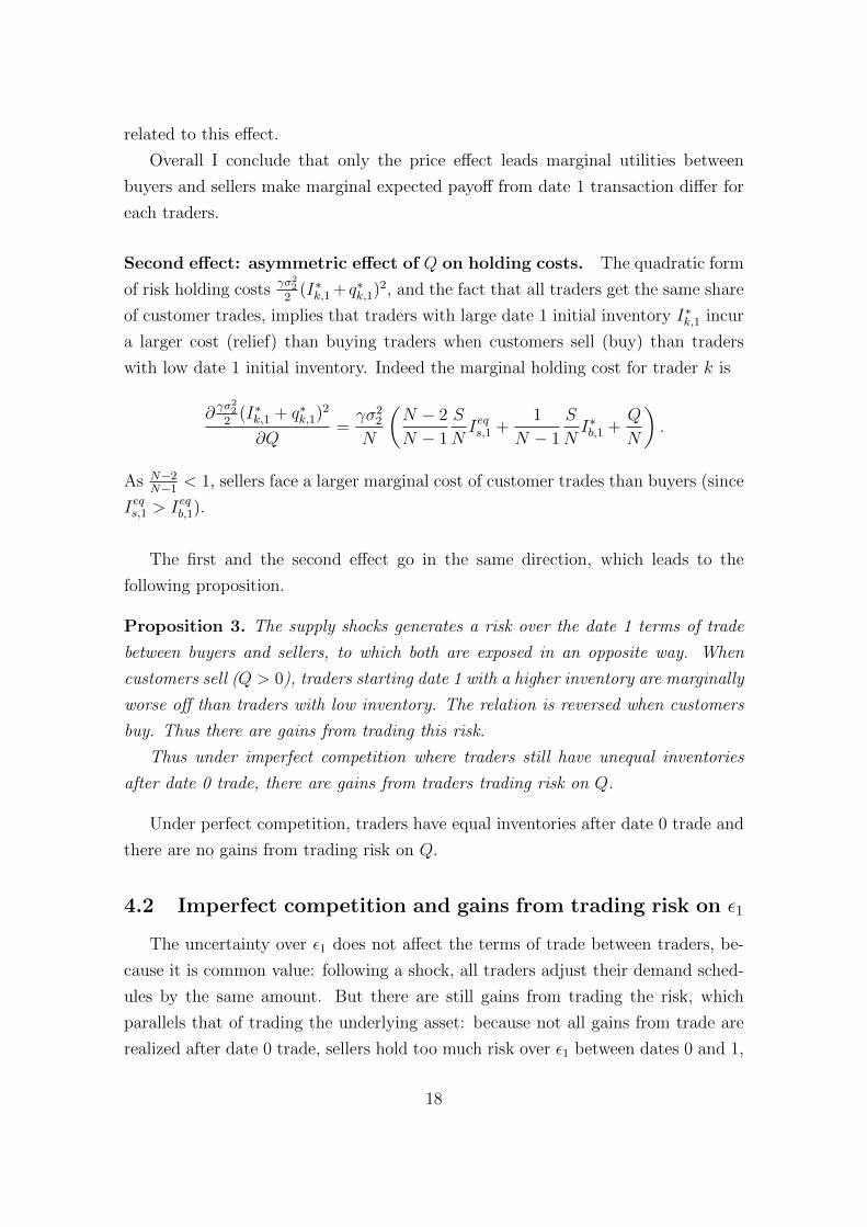
The date-0 certainty equivalent of wealth is (see proof in appendix B.4.1)

cW fk,0(qk,0, xk) = Vk + Sk,0(qk,0) + bSk,1(qk,0)

+ (bp1 � f0)xk � ���21 + (1� z)�2

2

�Ik,1xk �

�

2

✓�21 +

1� z

↵�22

◆x2k,

(5.1)

where bp1 is a risk-adjusted expectation of date-1 price p⇤1:

bp1 = v0 � ��22z

✓Ie1 +

N � 1

N � 2E0

Q

N

�◆

As in (3.8), Vk is the mean-variance certainty equivalent of wealth with trader k’s

initial inventory position Ik,0, bSk,0 and bSk,1 are trader k’s shares in date 0 and date

1 transaction surpluses in the underlying asset. The second line in 5.1 is the risk-

adjusted payo↵ of futures. It consists first in an expected payo↵ xk(bp1 � f0), which

depends on the trader’s trade. It also includes a hedging term in Ik,1xk (selling

futures, xk < 0, hedges against large inventory risk Ik,0 > 0), and a term in x2k that

reflects the riskiness of the futures payo↵.

Futures contracts payo↵ is open to influence, which shows up in the term xk(bp1�f0) in (5.1): a trader buying the futures contract would like a high underlying price

at date 1, and conversely. As noted in Section 4.3, this goes through the term in Ie1 .

To influence the price, a trader buying futures would like to sell massively at date 1

to make p⇤1 increase. In the limit, such an investor could sell the underlying asset at

date 0 only to re-purchase it at date 1, provided that the costs of doing so are o↵set

by a higher payo↵ on the derivative position. A trader selling the futures would like

to do the converse.21In appendix A, I solve the competitive benchmark with futures. At date 0, these contracts are

perfect substitutes with the underlying asset. Formally, from the first order conditions I cannotdeduce well-defined demand schedules for the futures and the underlying asset. This illustrates theredundancy of futures in a perfectly competitive setting: models based on the Theory of Storagewith perfect competition (Williams and Wright 1991, Routledge et al. 2000) also find that futuresare redundant with the underlying commodity.

20

There are two costs of influencing futures payo↵ in this way. First, the cost

of holding the excess or deficit position in the underlying asset and in the futures

contract from date 0 to date 1 (�21 in the model). Second, the uncertainty on date-1

price entailed by uncertainty on the supply shock Q. When these two costs are low,

the profit function 5.1 is not concave anymore, which means the following.22

Lemma 1. The certainty equivalent of wealth 5.1 is concave if and only if �2q is

above a threshold s(�21). This threshold decreases with �2

1.

When �2q is below s(�2

1), the certainty equivalent of wealth is not concave: a

trader with certainty equivalent of wealth 5.1 would try to achieve arbitrarily large

profit by submitting an arbitrarily large demand for the underlying asset, and an

opposite and even larger demand for the futures.

Traders’ strongest incentive is thus not to allocate trades to minimize date 0 and

date 1 buying or selling pressure anymore, but to trade in the spot market in order

to raise the futures payo↵ by a↵ecting date-1 price. In what follows, I assume that

�2q > s(�2

1).

5.2 Equilibrium definition

I assume imperfect competition in both the underlying asset and futures mar-

kets. Therefore, trader k takes the impact of trade in each market on both prices

simultaneously. To solve the equilibrium, I apply methods from Malamud and Ros-

tek (2017), which extends the method used without futures to a setting with several

assets. A 2⇥ 2 matrix of price impacts ⇤k,0 replaces the scalar price impact �k,0 of

Section 3, and the equilibrium condition becomes:

8<

:⇤s,0 = (B(⇤b,0 + �⌃f )�1 + (S � 1)(⇤s,0 + �⌃f )�1)�1

⇤b,0 = ((B � 1)(⇤b,0 + �⌃f )�1 + S(⇤s,0 + �⌃f )�1)�1. (5.2)

where the 2⇥2 matrix ⌃f is given in the appendix. As in Section 3.2, given that bSk,1

depends on p⇤1 which itself depends on other traders’ date-0 equilibrium trades in

the underlying asset, a trader’s demand schedules also depend on these quantities,

which have to coincide with actual equilibrium quantities.

22This does not necessarily imply that an equilibrium does not exist in the case above, even ifthe profit function is not quasi-concave (the graph of cW f

k,0 is a hyperbolic paraboloid): posting anarbitrarily large demand in both assets also entails arbitrarily large transaction costs at date 0. Ileave the question of equilibrium existence to future research.

21

Definition 3. Demand schedules q⇤k,0(p0, f0) in the underlying asset and x⇤k(p0, f0)

in futures contracts, and spot price p⇤0 and futures price f ⇤0 are an equilibrium if:

• demand schedules q⇤k,0(p0, f0) and x⇤k(p0, f0) maximize (5.1);

• price impacts matrices ⇤b,0 and ⇤s,0 satisfy (5.2);

• quantities qek,0 satisfy 3.11;

• market clearing conditions (2.2) and (2.3) hold.

5.3 The failure of futures payo↵ manipulation

At date 1, whatever equilibrium trades, the price (3.6) is unchanged by futures

trading: p⇤1 depends on traders’ average date 1 inventory

I1 =S

N(Is,0 + qs,0) +

B

N(Ib,0 + qb,0)

=S

NIs,0 +

B

NIb,0 ⌘ I0,

by market clearing at date 1 (equation (2.4)). One could have applied market clear-

ing to recognize I1 = I0 from the beginning, which would have changed the results.

But applying market clearing in this way is peculiar to the situation where buyers

and sellers share the same risk aversion parameter: with di↵erent risk aversions pa-

rameters, the date-1 price would be a↵ected by date-0 trades (Malamud and Rostek

2017).The following proposition shows that the underlying date-0 price is also not

a↵ected by futures trading. It also derives the futures price.

Proposition 4. The underlying asset price p⇤0 is equal to the price without futures:

p⇤0 = pn0 . (5.3)

The futures price is

f ⇤0 = v0 � �(�2

1 + �22)I0 �

N � 1

N � 2��2

2z E0

Q

N

�. (5.4)

The proof is in the appendix. There is no inventory risk premium associated

with futures, because the contract is in zero net supply. I also show in an online

appendix C that with futures whose payo↵ cannot be influenced, spot and futures

prices are exactly the same.

22

One could expect that more buyers implies more upward price pressure and

vice-versa. This is not the case: the underlying price, the futures price and thus the

forward-spot spread do not depend on the relative number of buyers and sellers, in

spite of e↵orts of both sides to impact them. Ultimately, this stems from the fact

that risk aversions, i.e. elasticities, on both sides are the same. Given the static

results by Malamud and Rostek (2017), it is likely that prices would depend on the

numbers of buyers and sellers with heterogenous risk aversions.

5.4 Equilibrium trades with futures

While the underlying price does not change, equilibrium trading patterns do

change with the introduction of futures. The following proposition establishes first

that sellers of the underlying asset buy futures, i.e. choose negative hedge ratios.

Proposition 5. If �2q is su�ciently large with respect to �2

1, an equilibrium with

futures exists and is unique. In the equilibrium with futures, sellers of the underlying

asset purchase futures to buyers of the underlying:

q⇤k,0 =1

1 + Afqck (5.5)

q⇤k,1 =Af

1 + Af⇥ N � 2

N � 1⇥ qck +

Q

N(5.6)

x⇤k = hf

✓q⇤k,1 �

Q

N

◆(5.7)

where hf is negative. qck is the competitive quantity traded at date 0 (A.12), and

Af > 0 is the date 0 rate of trade delay with futures contract and depends on N , on

z and on the ratio �21/�

22.

The quantity of futures traded x⇤k is equal to the quantity deferred to date 1,

q⇤k,1�Q/N , times the hedge ratio hf .23 As stated in Section 4, if the hedging motive

dominated, traders would choose positive hedge ratios, i.e. trade futures and the

underlying asset in the same direction. But in equilibrium, hedge ratios are negative.

For futures buyers, influencing futures payo↵ involves raising date-1 price, thus

purchasing more or selling less at date 1; and likely preparing this at date 0 by

selling more, or purchasing less. The opposite holds for futures sellers. Who should

23The hedge ratio is to be computed with respect to expected date-1 quantity (minus the supplyshock), not to date-0 quantity or date 0 inventory. This general form also holds for my theoreticalnon-manipulable futures in the online appendix C, except that the hedge ratio is positive.

23

be futures buyers? If these were underlying buyers, they would carry too little risk

on ✏1, and sellers too much, from date 0 to date 1. Thus buyers and sellers all prefer

that futures buyers are underlying asset sellers, which is opposite to hedging would

require. The following proposition, proven in the appendix, confirms this.

Proposition 6. Futures accelerate trading in the underlying asset:

|qnk,0| < |q⇤k0|

|qnk,1| > |q⇤k,1|

This is because the rates of trade delay are such that A > Af .

Influence on date-1 price is more likely to fail if this price is more uncertain. Con-

sider uncertainty associated with Q first: if �2q increases, trying to raise date-1 price

(for a futures seller) is more likely to be o↵set by date 1 customers pushing the price

downward. Thus the payo↵ influence motive for trading decreases as �2q increases.

Moreover, as stated in Section 5.1, another cost of trying to influence futures pay-

o↵ is the risk on ✏1, which entails a more uncertain futures payo↵. The following

proposition, proven in the appendix, states that this is reflected in quantities.

Proposition 7. The quantity of futures traded |x⇤k| decreases as �2

q increases, and

shrinks to zero as �2q diverges to infinity.

The quantity of futures traded also decreases as �21 increases.

This proposition thus states that traders trade less futures when they have more

hedging needs. The intuition is clear, since when they try to influence futures

payo↵, traders do not hedge with futures, but choose a naked exposure to date-1

price through the futures contract.

5.5 The perfect competition limit: futures are not traded

Here I show that when the number of traders grows to infinity, futures position

and open interest shrink to zero, justifying the claim that imperfect competition

creates a demand for futures.

To look at the limit when N grows to infinity, I have to care about whether N

grows because one adds an overwhelming proportion of buyers or of sellers, or if

some balance between buyers and sellers is kept. Formally, the latter means that

the ratio B/S remains finite and stays away from zero.

24

A second issue is that to isolate the pure e↵ect of imperfect competition, I have to

care about adding traders while keeping total inventories constant: for instance, if I

added sellers all with the same inventory Is,0, as S would grow, the collective sellers

position would be SIs,0, which would grow as well. This is undesirable because

it would mix the e↵ect of increased competition with the e↵ect of an increase in

aggregate supply or demand in the underlying asset. Thus I consider some fixed

collective initial inventories Is for sellers, to be split equally across sellers, and Ib for

buyers, to be split equally across buyers.

Corollary 1. As N grows to infinity, holding average market inventory constant,

and if the ratio B/S of the number of buyers to the number of sellers remains finite

and does not approach zero,

• individual traders positions x⇤k in futures contracts shrink to zero,

• the total quantity of futures traded (open interest) B|x⇤b | = S|x⇤

s| shrinks to

zero.

The second part is not implied by the first: one could imagine that individual

traders position shrink to zero just because some fixed quantity of futures is split

across more and more traders.

6 The welfare impact of futures

In this section, I derive traders’ equilibrium welfare and spell the trade-o↵ be-

tween higher trading speed and hedging benefits of futures, observing that trading

the futures and the underlying asset in opposite directions implies a welfare loss.

Then I show why a higher trading speed benefits to all traders. Finally, I show

that overall, futures decrease welfare in this model because traders try to influence

futures payo↵.

For simplicity, in this section I assume E0[Q] = 0.

6.1 Traders’ welfare with or without futures

Without futures Plugging equilibrium prices and quantities in the certainty

equivalent of wealth 3.8 leads to

cW nk,0 = Vk + Sk,0(A) + bSk,1(A)

25

where Sk,0(A) and bSk,1(A) are the equilibrium shares of date 0 and date 1 surpluses

that accrue to trader k when the rate of trade delay is A:

Sk,0(A) =�(�2

1 + �22)

2

1�

✓A

1 + A

◆2!(qck)

2

bSk,1(A) =↵

2��2

2z

✓A

1 + Aqck

◆2

With futures. Similarly, plugging relevant equilibrium quantities into date 0 cer-

tainty equivalent of wealth 5.1 yields

cW fk,0 = Vk + Sk,0(Af ) + bSk,1(Af )

+ �hf

" 1� hf

2

!�21 +

↵� hf

2

!1� z

↵�22

#✓Af

1 + Af

◆2

(qck)2 (6.1)

where hf = N�2N�1hf . It is easy to see that when the hedge ratio hf is negative,

which corresponds to traders trading futures and the underlying asset in opposite

directions, the part associated with derivatives becomes negative. Thus the following

lemma.

Lemma 2. If traders choose a negative hedge ratio, i.e. buy futures when they sell

the underlying and vice-versa, they make a gross loss.

Intuitively, as suggested by the discussion of Section 4 if traders buy futures

when they sell the underlying asset, they increase their exposure to the supply

shock Q, and retain too much of the underlying risk on ✏1. However, this goes on

with accelerated trading of the underlying asset, which increases welfare as shown

in the following subsection.

6.2 Delaying trade decreases traders’ welfare

Intuitively, lower quantities traded at the same prices suggests surplus from trans-

actions decreases when more trade is postponed to date 1. The following proposition

checks that this is the case, and allows to uncover the di↵erent e↵ects that cause

the welfare to decrease.

Trading slows down whenever the date 0 rate of trade delay A increases, so that

the date-0 quantity dcreases and date-1 quantity increases. Thus I measure the e↵ect

of trading speed on trader k’s surplus through the marginal e↵ect of an increase in

A.

26

Proposition 8. Surplus from date 0 and date 1 transactions decrease as the rate A

increases, as indicated by the first term of the following:

@(Sk,0 + bSk,1)

@A= ��(�2

1 + (1� ↵z)�22)

A

(1 + A)3�qck,0

�2 � (1� ↵)��22z E0

Q

N

�qck,0

The second term shows how it a↵ects the distribution of surplus between buyers and

sellers.

Welfare decreases for three reasons apparent in the first term

1. Holding cost e↵ect: when �21 > 0, sellers hold more risk from date 0 to date 1,

which is costlier to them.

2. Uncertainty over the supply shock �2q makes date 1 surplus is more uncertain,

thus decreases its ex ante value; the e↵ect shows up through a lower z.

3. Imperfect competition: given that ↵ < 1, risk sharing is ultimately reduced

given z.

The second term is non-zero if ↵ < 1, which is always the case if N is finite: thus it

stems from imperfect competition. It is positive if date 1 customers are expected to

sell (E0[Q] > 0) and trader k is a seller (qck,0 < 0), and vice-versa: traders trading in

the opposite direction to date 1 customers are better o↵ postponing trade.

6.3 Net e↵ect of futures introduction

In the equilibrium with futures, trading is faster than without futures, which

means a welfare gain. However, traders trade futures in the opposite direction to

what they would do if they did it for hedging purposes: this implies a welfare loss.

Which force dominates is a priori unclear. The following theorem shows that the

negative e↵ect dominates.

Theorem 1. For all N � 3, all �2q � 0 and all �2

1 > 0, introducing futures decrease

traders welfare:

cW fk,0 <

cW nk,0.

6.4 The welfare of liquidity traders

The date 1 supply shock Q is a net demand posted by traders whose prefer-

ences are not modelled, which in principle precludes computation of their welfare.

27

However, it is possible to run simple welfare comparisons for them, because their

demand is inelastic: modelled traders always absorb all their quantities at a given

price. Thus liquidity traders’ welfare is measured by the price at which their trades

are executed. The date-1 equilibrium price is una↵ected by the presence of futures:

thus date 1 liquidity traders’ welfare is unchanged.

7 A deviation from the law of one price: the

futures-spot basis

Comparing spot and futures prices in equations (5.3) and (5.4), one easily sees

that there is a non-zero spread (“basis”) between the spot and futures price:

f ⇤0 � p⇤0 = � 1

N � 2��2

2z E0

Q

N

�(7.1)

which di↵ers from zero as long as E0[Q] 6= 0. This basis does not stem from the fact

that traders seek to influence futures payo↵: in the online appendix C, I show that

with more abstract contracts where payo↵ influence is impossible the equilibrium

prices are the same.

The dependence of the spot price and of the futures prices on E0[Q] reflect two

di↵erent e↵ects and comes in each price with di↵erent coe�cients. For the spot price,

the dependence comes from the certainty equivalent of date-1 surplus bSk,1, expressed

in equation (3.10) and that appears without futures. When traders anticipate sales

by customers (E0[Q] > 0), for instance, they expect to purchase the asset at a low

price at t = 1. Both to reduce their holding costs and in the hope of realizing a

speculative profit by selling at a high price to repurchase at a low price, traders

reduce their demands at t = 0. The coe�cient in front of ��22z E0[Q/N ] in the

marginal wealth of an additional unit of the underlying asset is 1. The e↵ect is

symmetric for E0[Q] < 0. The dependence of the futures price in E0[Q] simply

reflects the expected payo↵ from the futures contract, which is xk(bp1 � f0) in (5.1).

Consistently with the expression of date-1 price, the coe�cient of ��22z E0[Q/N ] is

(N � 1)/(N � 2) > 1.

The basis may appear surprising in a context where there are no trading con-

straints, because traders leave an arbitrage opportunity on the table. This may seem

inconsistent with equilibrium:24 when E0[Q] > 0, the futures is below the spot, so

24The basis is often justified by storage costs (for commodities markets) and interest rate, which

28

that it is profitable to enter a long position in the futures contract paying o↵ p⇤1�f ⇤0

and sell the underlying asset giving p⇤0; at date 1, the futures pays o↵ and the arbi-

trage strategy would imply re-purchasing the asset at price p⇤1, yielding an overall

profit p⇤0 � f ⇤0 for sure. When E0[Q] < 0, it is profitable to buy the underlying asset

and sell the futures.

But such an arbitrage strategy is in fact opposite to traders’ optimal strategy.

To see it, compare the equilibrium certainty equivalents of wealth for buyers and

sellers. The following proposition says that sellers are better o↵ when the futures

price increases with respect to the spot price, which means that they are better o↵

by selling the asset at a lower price than the price at which they enter the futures

position.

Proposition 9. Sellers have greater equilibrium utility than buyers if and only if

S

N< u+ v ⇥ (f ⇤

0 � p⇤0),

where v > 0. Otherwise buyers have greater equilibrium utility.

The proof is in the appendix. This proposition therefore indicates if traders were

to choose between becoming a buyer or a seller by building inventories or inventory

deficits before the date 0 market opens,25 taking E0[Q] / f ⇤0 � p⇤0 as given, more

traders would choose to become sellers of the underlying asset, and buyers of futures,

if the futures price f ⇤0 increased with respect to the spot price p⇤0.

The intuition behind this apparent paradox is the following. When f ⇤0 > p⇤0, the

date-0 spot price and the expected date-1 spot price are at a higher level than when

f ⇤0 < p⇤0, because E0[Q] < 0: the terms of trade between buyers and sellers are more

favorable to sellers, which raises the welfare associated with selling the underlying

asset. In addition, the futures expected payo↵ bp1 � f ⇤0 does not depend on E0[Q],

because an increase in the expected date-1 price is reflected one-for-one in the fu-

tures price: thus traders’ welfare depends on E0[Q] only through the date-1 surplusbSk,1, and not through the futures payo↵: a higher basis only reflects the impact of

a higher spot price on traders’ welfare.

The existence of a spread between two assets with identical payo↵ is usually

are both normalized to zero in the present paper.25A simple setting would start with all traders having the same inventory position I, with traders

observing E0[Q], then they would simultaneously choose to build additional inventory for a fixedquantity �I > 0 at some cost c.

29

explained by constraints that preclude traders in one market to trade with traders

in another market26, together with constraints on arbitrageurs: valuations for the

asset in the two markets di↵er, so do the prices. In these models, arbitrage allows

for the realization of gains from trade and tends to improve market e�ciency. 27

The present model gives another explanation for the divergence of prices of sim-

ilar assets, which is clearly not exclusive of constraints. Equilibrium divergence of

prices of similar asset should not be surprising in an imperfectly competitive setting:

a textbook monopolist prices its good above marginal cost, thus optimally leaves ar-

bitrage opportunities on the table - it is possible to pay the marginal cost to produce

a unit of the good, and sell it at a price above the cost. With more competition,

the market price for the good would be closer to producers’ marginal cost. Here like

in traditional models of industrial organization, the spread also goes to zero as the

number of traders N increases, i.e. as the market becomes more competitive.

Arbitrage opportunities that emerge because of imperfect competition have very

di↵erent implications than those that emerge because of constraints. While more

arbitrage directly benefits traders facing the constraints in the first place, this is not

the case here. In the present setting, arbitrage by traders is a zero-sum game: if

one trader exploits the arbitrage opportunity, traders on the opposite side of both

trades make a corresponding loss. It is therefore unlikely that the latter traders

would accept such trade. This is in contrast with situations where some traders are

constrained not to participate in one market: in these situations, arbitrageurs buy

to traders who are eager to sell, and sell to traders who are eager to buy, so that

everyone is better o↵.28 This does not mean that arbitrage would overall decrease

welfare: arbitrage for instance could bring more competition, which would presum-

ably increase welfare. But this would go through indirect e↵ects. Full modeling of

arbitrageurs would be interesting for future research.

26In Gromb and Vayanos (2002, 2010, 2018), the constraint is exogenous. In Biais et al. (2019),the constraint is of incentive-compatibility.

27In commodities markets, the theory of normal backwardation is often stated as a variant onthis theme: in these theories, speculators take the opposite side to traders who need to hedgefuture production. Speculators require a risk premium for this service. If speculators were allowto trade in the spot market, they would hedge their futures position with an opposite position inthe spot market, so that they would be less exposed to the risk on futures; if they chose perfecthedge, the risk premium would disappear.

28Constraints limiting the arbitrage activity may make arbitrageurs take ine�cient positions asshown by Gromb and Vayanos (2002), but if these constraints were not there, arbitrage wouldunambiguously raise welfare.

30

8 Conclusion

In this paper, I provide an equilibrium model where futures contracts are traded

even if no trader is constrained to trade in the future, and I study pricing and

welfare implications. If traders were wiling to trade today in the spot market, they

would be hedged against future price movements and thus would not need to trade

futures. But when traders are imperfectly competitive, traders choose to postpone

some trades that would be profitable to execute today in order to minimize their

overall price impact. By doing this, they expose themselves to the risk that the at

which they will trade tomorrow moves against them. As buyers of the asset fear

that the price goes up and sellers fears that the price goes down, there are gains

from trading this risk by using futures.

However, once futures are introduced, traders also want to trade the underlying

asset at futures maturity in order to influence the futures contract payo↵, which

is the di↵erence between the underlying asset price at futures maturity, and the

futures price: buyers of the futures contract want to raise the underlying asset price,

and sellers of the futures want to decrease it. In this setting, they try to impact

tomorrow price by trading in the underlying asset.

I show that in equilibrium, this incentive dominates the hedging demand for

futures: contrary to what hedging predicts, sellers of the underlying asset buy the

futures to buyers of the underlying asset, and less trade in the underlying asset

is delayed. Sellers of the underlying asset sell more initially in order to sell less

tomorrow, which would raise the price. Buyers do the opposite. Moreover, traders

attempts to manipulate prices fail in equilibrium, because buyers and sellers pull

the price in opposite directions.

Then I assess traders’ welfare e↵ects of introducing futures. Attempts to manip-

ulate futures payo↵ have a positive and a negative e↵ect. The positive e↵ect is that

trading in the underlying asset is faster while prices are unchanged, so that sellers

carry less of the asset: there is a better allocation of risk associated with the under-

lying asset. The negative e↵ect is that traders choose negative hedge ratios: trading

futures in opposite direction to hedging leaves traders more exposed to tomorrow

price risk. Overall, I prove that futures decrease all traders’ welfare. However, if

manipulation was precluded by o↵setting spot price manipulation one-for-one on

the futures price, traders would trade futures for hedging, and their welfare would

increase.

Finally, I examine how imperfect competition shapes spot and futures prices,

31

and the basis between the two. This is surprising as bases between two assets with

similar payo↵s are usually explained with some market segmentation, which is absent

in this model.

The futures price can be above or below the spot price, depending on expectations

of the supply shock, i.e. depending on expectation of date-1 price. The basis shrinks

to zero as competition becomes perfect. I also show that sellers of the underlying

asset have greater welfare with respect to sellers when the futures price is more

above the spot price, meaning that in equilibrium they sell the underlying asset

more cheaply than they buy the futures: this is surprising given that an arbitrageur

doing the same would be hurt. While I do not model arbitrageurs, this suggests

ambiguous welfare e↵ects of arbitrage in such a context.

32

Appendix

A Perfect competition benchmark

A.1 No futures

Equilibrium definition. I look for competitive equilibria defined as sets of de-

mand schedules (q⇤i,0(p0), q⇤k,1(p1)) (k = b, s) and equilibrium prices pc0, p

c1 such that:

1. All traders are price-takers;

2. Trader k’s date 1 demand schedule q⇤k,1(p1) maximizes his/her expected utility

of terminal wealth Wk given information available at date 1;

3. For each trader k, date 0 demand schedules q⇤k,0(p0, f0) maximize their ex-

pected utility of terminal wealth Wk given information available at date 0 and

anticipated equilibrium outcomes at date 1;

4. The market clearing conditions (2.2) and (2.4) hold.

Again I make the slight abuse of notation that that symmetry of traders of class

i is included in the definition, while it is in fact an equilibrium outcome. I look for

equilibria by backward induction.

A.1.1 Date 1

Traders k maximize over qk,1 her expected utility. Given that the only uncertainty

is on the normally distributed variable ✏2, the certainty equivalent of wealth is:

fWk,1 = Ik,0v1 + qk,0(v1 � p0) + qk,1(v1 � p1)��

2�22(Ik,1 + qk,1)

2. (A.1)

As the utility function is increasing, all happens as if trader k maximized the cer-

tainty equivalent fWk,1 of her wealth. From the first order condition of this maxi-

mization problem one easily derives the optimal competitive demand schedule:

qck,1(p1) =v1 � p1��2

2

� Ik,1 (A.2)

Demand increases when the expected terminal payo↵ v1 is larger with respect to the

purchase price p1, when traders’ risk aversion � is low, and when the terminal payo↵

33

variance �22 is low. Plugging optimal demands into the market clearing condition

(2.4), it is straightforward to derive the equilibrium price

pc1 = v1 � ��22

Q⇤c

2(A.3)

with Q⇤c =

S

NIs,1 +

B

NIb,1 +

Q

N

Notice that with date 0 market clearing condition (2.2), one has SN Is,1 +

BN Ib,1 =

SN Is,0+

BN Ib,0. The equilibrium price therefore equals the expected value of the asset

minus a risk premium that increases if risk aversions increase, if the uncertainty �22

over the asset terminal payo↵ v increases, and if the quantity held by traders after

date 1 trade increases. In particular, if customers are net sellers (Q > 0), then the

equilibrium price decreases and vice versa, which is intuitive.

Plugging equilibrium price (A.3) into optimal demand schedule (A.2), one gets

the equilibrium quantities purchased by buyers and sellersare:

qcb,1 =S

N(Is,1 � Ib,1) +

Q

N, qcs,1 =

B

N(Ib,1 � Is,1) +

Q

N(A.4)

After date 1 trade, all traders thus hold

Ib,1 + qcb,1 = Is,1 + qcs,1 =S

NIs,0 +

B

NIb,0 +

Q

N(A.5)

A.1.2 Trader valuation of the surplus of date 1 trade

After date 1 trade, from A.1, trader k’s certainty equivalent of wealth can be

decomposed as

fWk,1 = Ik,0v1 + qk,0(v1 � p0)���2

2

2(Ik,0 + qk,0)

2 + Sck,1 (A.6)

with Sck,1 = qck,1(v1 � pc1)�

✓��2

2

2(Ik,1 + qck,1)

2 � ��22

2(Ik,1)

2

◆(A.7)

The first terms are the classical mean-variance value of date 0 inventory position

after date 0 trade.

Sc1 is the net surplus of date 1 transaction. It is the sum of two terms: qck,1(v1�pc1)

is the expected payo↵ from the trade, while the di↵erence in bracket is the impact

of the change in trader k’s inventory position on her risk holding cost. Rearranging

34

the expression of Sck,1 above leads to:

Sck,1 =

��22

2

�qck,1

�2(A.8)

Crucially, Sck,1 can also be influenced by date 0 trading choice qk,0, as revealed by

expression A.4 of date-1 quantity. As seen shortly, under perfect competition, this

impacts only date-0 equilibrium price. Under imperfect competition, this impacts

both date-0 equilibrium price and quantity.

Plugging A.8 into A.7 and taking the certainty equivalent with respect to both

✏1 and Q using lemma 5 in the appendix,29 one gets the date 0 certainty equivalent

of wealth for trader k:

fWk,0 = Ik,0v0 + qk,0(v0 � p0)��

2(�2

1 + �22)(Ik,0 + qk,0)

2

+��2

2

2zc�E0[q

ck,1]

�2+ cst (A.9)

with qck,1 =Q⇤

c

2� Ik,0 � qk,0 and zc =

1

1 + �2�22�

2q

A.1.3 Date 0

Optimal demand schedules. The optimal demand qck,0(p0) maximizes the cer-

tainty equivalent of wealth (A.9). The problem is solved by the unique solution to

the following first order condition:30

v0 � p0 = �(�21 + �2

2)�Ik,0 + qck,0(p0)

�� ��2

2zc⇥E0[Q

⇤c ]�

�Ik,0 + qck,0(p0)

�⇤

Rearranging leads to

qck,0(p0) =v0 � p0

�(�21 + (1� zc)�2

2)� �2

2

�21 + (1� zc)�2

2

zc E0

Q⇤

c

2

�� Ik,0 (A.10)

The optimal demand is the sum of a quasi hold-to-maturity demand (first term),

analogous to the two periods demand (A.2), and the short term profit demand, that

appears as an arbitrage demand (second term). Both terms are impacted by the

uncertainty about the liquidity shock �2q .

29Sck,1 is quadratic in Q, and the certainty equivalent takes this into account.

30It is straightforward to check that the problem is strictly concave, as zc < 1.

35

Equilibrium. The equilibrium prices and quantities are stated in the following

proposition, proven in the appendix.

Proposition 10. The equilibrium price is

pc0 = v0 � �(�21 + �2

2)I0 � ��22zc E0

Q

N

�(A.11)

where I0 = SN Is,0 +

BN Ib,0 is the average initial inventory across traders. The risk

premium is the sum of a hold-to-maturity component (second term), and of an short-

term arbitrage component (third term) that is proportional to the expected date 1

liquidity shock: the price is higher when customer purchases are expected (E0[Q] < 0)

and vice versa. The sensitivity to the date 1 liquidity shock decreases as uncertainty

about it increases.

Equilibrium trade and post-trade inventories are

qcb,0 =S

N(Is,0 � Ib,0) qcs,0 =

B

N(Ib,0 � Is,0) (A.12)

qcb,1 = qcs,1 =Q

N(A.13)

and all traders end up with the average inventory I0 ⌘ S/NIs,0 + B/NIb,0. Risk

sharing is Pareto optimal.

Inventories are equalized right after date 0 trade: all intertrader gains from trade

are realized at date 0. By market clearing, as date 1 customers are price inelastic,

the short term capital gain demand has no impact on the quantities traded and all

e↵ect goes in the price.

Traders’ welfare. Plugging equilibrium price (A.11) and quantities (A.12) and

(A.13) into the certainty equivalent of wealth (A.9) gives

fW cb,0 = Ib,0v0 �

�(�21 + �2

2)

2(Ib,0)

2 +�(�2

1 + �22)

2

�qcb,0

�2+

��22

2zc

✓E0

Q

N

�◆2

� 1

2�ln(zc)

(A.14)

A.2 Perfect competition: redundancy of futures

Here I add futures contracts, to show that they are perfect substitutes to the

underlying asset under competition. To do this I add the futures payo↵ xk(v1 � p⇤1)

36

to the date 1 certainty equivalent of wealth (A.7), rearrange and take the date 0

certainty equivalent of wealth to find

fW c,fk,0 = Ik,0v0 + qk,0(v0 � p0)�

�

2(�2

1 + �22)(Ik,0 + qk,0)

2 +��2

2

2zc�E0[q

ck,1]

�2

+ xk(ep1 � f0)��

2

��21 + (1� zc)�

22

�(x2

k + Ik,1xk) (A.15)

with

ep1 = v0 � ��22zc

✓I0 + E0

Q

N

�◆

and qck,1 is the date-1 equilibrium quantity A.13. Di↵erentiating (A.15) with respect

to both trade in the underlying asset qk,0 and futures xk, and treating prices including

ep0 as constants, I find the following first-order condition:

v0 � p0

v0 � f0

!= �

��21 + (1� zc)�

22

� 1 1

1 1

! qk,0

xk

!+ cst

Clearly, this equation cannot be inverted to get demand schedules. Thus the follow-

ing proposition.

Proposition 11. In the competitive equilibrium with futures, quantities traded are

indeterminate: futures are redundant with the underlying asset.

This result illustrates the economic puzzle of futures trading when the underlying

asset is also traded. As I shall show in Section 5, under imperfect competition,

futures are not redundant anymore.

B Proofs

B.1 Proof of proposition 10

Plugging optimal demand (A.10) into the market clearing condition (2.2), one

gets

1

�

v0 � p⇤0�21 + �c�2

2

� �22zc

�21 + �c�2

2

E0[Q⇤c ] = 0

37

Rearranging one gets the equilibrium price formula (A.11). Plugging the equilibrium

price formula into the optimal demand schedule (A.10), one gets

Ik,0 + q⇤k,0(p⇤0) =

�(�21 + �2

2)I0 + ��22zc E0

⇥QN

⇤

�(�21 + �c�2

2)� �2

2

�21 + �c�2

2

zc E0 [Q⇤c ]

=1

�21 + �c�2

2

��21 + �2

2 � zc�22

�I0

= I0

The optimality of risk sharing comes from the competitiveness of the market

(first welfare theorem).

B.2 Proof of proposition 2

B.2.1 Demand schedules

From proposition 1, the post-trade certainty equivalent of wealth at date 1 is

given by the following lemma, proven in the appendix.

Lemma 3. Trader k’s interim expected utility is � expn��cWk,1

o, where cWk,1 is

the interim certainty equivalent of wealth given by:

cWk,1 = Ik,0v1 + qk,0(v1 � p0)���2

2

2(Ik,1)

2 + ↵��2

2

2

✓�

�Q⇤ � Ik,1

◆2

(B.1)

= Ik,0v1 + qk,0(v1 � p0)���2

2

2(Ik,1)

2 +N

N � 2

��22

2

�q⇤k,1

�2(B.2)

where ↵ = N(N�2)(N�1)2 = 1� 1

(N�1)2 .

Proof. Plugging equilibrium price (3.6) and quantities (3.5) into the date 1 certainty

equivalent of wealth (A.1), one gets

cWk,1 = Ik,0v1 + qk,0(v1 � p0)���2

2

2(Ik,1)

2 + q⇤k,1(v1 � p⇤1)���2

2

2

⇣�Ik,1 + q⇤k,1

�2 � (Ik,1)2⌘

38

Recognizing v1�p⇤1��2

2= N�1

N�2q⇤k,1 + Ik,1 and rearranging one get

cWk,1 = Ik,0v1 + qk,0(v1 � p0)���2

2

2(Ik,1)

2

+ q⇤k,1��22

✓N � 1

N � 2q⇤k,1 + Ik,1

◆� ��2

2

2

�2Ik,1 + q⇤k,1

�q⇤k,1

= Ik,0v1 + qk,0(v1 � p0)���2

2

2(Ik,1)

2 +

✓N � 1

N � 2� 1

2

◆��2

2

�q⇤k,1

�2

which leads to the desired formulas.

It is then possible to compute the certainty equivalent of wealth at date 0.

Lemma 4. The date 0 certainty equivalent of wealth for a buyer is:

cWb,0 = Ii,0v0 + qk,0(v0 � p0)��(�2

1 + �22)

2(Ik,1)

2 +1

2

N

N � 2��2

2z�E0

⇥q⇤k,1

⇤�2(B.3)

= Ik,0v0 + qk,0(v0 � p0)��(�2

1 + �22)

2(Ik,1)

2

+↵

2��2

2z

✓�

�E0

Q

N

�+

S

NIes,1 +

B � 1

NIeb,1 �

N � 1

NIk,1

◆2

(B.4)

where z = (1 + �2�22�

2q )

�1and � = N�1

N�2�. Ie�i,1 and Iei,1 are the expectations of

average trader inventories after date 1 trade.

For sellers, replaceSN Ies,1 +

B�1N Ieb,1 with

S�1N Ies,1 +

BN Ieb,1 in (B.4).

Proof. Start from interim expected utility (B.2). Take the certainty equivalent with

respect to ✏1 first, which gives

cWk,0|Q = Ik,0v1 + qk,0(v1 � p0)��(�2

1 + �22)

2(Ik,1)

2 + ↵��2

2

2

✓�

�Q⇤ � Ik,1

◆2

Then take the certainty equivalent with respect to Q is given by the following lemma

Lemma 5. Let X ⇠ N (µ,⌃) a normal vector of dimension p (|⌃| > 0), and A

a symmetric matrix. Then one seeks to compute E[exp(��X 0AX)] where A is a

symmetric matrix.

Suppose I + 2�A⌃ is positive definite, then

E[exp(��X 0AX)] =1p

|I + 2�A⌃|exp

���µ0(I + 2�A⌃)�1Aµ

39

Proof.

E[exp(��X 0AX)] =

Z

Rp

1p2⇡|⌃|

exp

⇢��x0Ax� 1

2(x� µ)0⌃�1(x� µ)

�dx

where dx ⌘ dx1dx2...dxp. One first computes

Q(x) = ��x0Ax� 1

2(x� µ)0⌃�1(x� µ)

= �1

2(x� µ)0(⌃�1 + 2�A)(x� µ)� 2�µ0A(x� µ)� �µ0Aµ

Suppose that (⌃�1+2�A) is the inverse of a covariance matrix, then the formula

will give almost the moment generating function of a normal variable with covariance

matrix [(I + 2�A⌃)⌃�1]�1 = ⌃(I + 2�A⌃)�1.

Ehe��X0AX

i=

e��µ0Aµ

p|I + 2�A⌃|

⇥Z

Rp

1p2⇡|⌃||I + 2�A⌃|�1

e�2�µ0A(x�µ)e�12 (x�µ)0[⌃(I+2�A⌃)�1]�1(x�µ)dx

=1p

|I + 2�A⌃|exp

���µ0(I + 2�A⌃)�1Aµ

For the (B.4), Q⇤ is an outcome of date 0 trade, as it depends on traders’ average

inventories in each class. Trader k’s trade has an impact on date his class’ average

date 1 inventory Ie1 since

Ie1 ⌘ 1

N

NX

l=1,l 6=k

Iel,i,1 +Ik,1N

=S

NIes,1 +

B � 1

NIeb,1 +

Ik,1N

if trader k is a buyer, and

Ie1 =S � 1

NIes,1 +

B

NIeb,1 +

Ik,1N

if trader k is a seller. I have used the fact that traders within a group (buyers/sellers)

play symmetric strategies.

Lemma 6. In equilibrium, all buyers submit the same optimal demand schedules as

40

follows:

q⇤b,0(p0) =N � 2

N � 1

v0 � p0

�(�21 + ��2

2)� Ib,0

�N � 2

N � 1z

�22

�21 + ��2

2

✓�

�E0

Q

N

�+

S

NIes,1 +

B � 1

NIeb,1

◆�(B.5)

and sellers submit a demand schedule obtained by replacingSN Ies,1 +

B�1N Ieb,1 with

S�1N Ies,1 + B

N Ieb,1 in (B.5). It depends on trader k’s expectation on other traders’

equilibrium trades.

Proof. Di↵erentiate the certainty equivalent of wealth (B.4) with respect to qk,0,

taking into account its price impact that is conjectured to be constant (and denoted

�k,0). Equating to zero to get the first-order condition for a buyer:

v0 � p0 = (�k,0 + �(�21 + �2

2))qk,0 + �(�21 + �2

2)Ib,0

+N � 2

N � 1��2

2z

✓�

�E0

Q

N

�+

S

NIes,1 +

B � 1

NIeb,1 �

N � 1

NIk,1

◆

= (�k,0 + �(�21 + ��2

2))qb,0 + �(�21 + ��2

2)Ib,0

+N � 2

N � 1��2

2z

✓�

�E0

Q

N

�+

S

NIes,1 +

B � 1

NIeb,1

◆

where

� = 1� N � 2

Nz 2 [0, 1].

It is thus straightforward to check that the second derivative of cWk0 is negative, so

that the problem is strictly concave. Using proposition 1 of Malamud and Rostek

(2017)

�k,0 =�(�2

1 + ��22)

N � 2

Plugging equilibrium price impacts �k,0 in the first order condition and rearranging,

one gets the desired formula.

41

B.2.2 Equilibrium price and quantities

The date 0 market clearing condition can be written:

v0 � p⇤0�(�2

1 + ��22)

= I0 +N � 2

N � 1z

�22

�21 + ��2

2

✓�

�E0

Q

N

�+

N � 1

N

✓S

NIes,1 +

B

NIeb,1

◆◆

By market clearing at date 0, SN Ies,1+

BN Ieb,1 =

SN Is,0+

BN Ib,0 ⌘ I0; in addition, recalling

�/� = N�1N�2 , one has

v0 � p⇤0 = �(�21 + ��2

2)I0 +N � 2

N��2

2zI0 + ��22z E0

Q

N

�

Recalling the definition of �, the equilibrium price is therefore:

p⇤0 = v0 � �(�21 + �2

2)I0 � ��22z E0

Q

N

�(B.6)

Plugging B.6 into the equilibrium demand schedule for buyers:

q⇤b,0 =N � 2

N � 1

I0 +

N � 2

N � 1z

�22

�21 + ��2

2

✓�

�E0

Q

N

�+

N � 1

N

✓S

NIes,1 +

B

NIeb,1

◆◆

�N � 2

N � 1z

�22

�21 + ��2

2

✓�

�E0

Q

N

�+

S

NIes,1 +

B � 1

NIeb,1

◆�

=N � 2

N � 1

S

N

Is,0 � Ib,0 +

1

N � 1

N � 2

Nz

�22

�21 + ��2

2

✓Ib,0 � Is,0 +

✓1 +

B

S

◆qeb,0

◆�

where the third line used the equilibrium condition qe2,0 = q⇤2,0 and market clearing

2.2, boiling down to q⇤s,0 = �B/S q⇤b,0. Given 1 +B/S = N/S, one gets:

✓N � 1

N � 2� N � 2

N(N � 1)

z�22

�21 + ��2

2

◆q⇤b,0 =

✓1� N � 2

N(N � 1)

z�22

�21 + ��2

2

◆S

N(Is,0 � Ib,0)

Notice that with � = 1� N�2N z,

1� N � 2

N(N � 1)

z�22

�21 + ��2

2

=�21 +

�1� N�2

N�1z��22

�21 +

�1� N�2

N z��22

> 0

This and rearranging leads to the desired equilibrium quantity:

q⇤b,0 =1

1 + A(�2q )

⇥ S

N(Is,0 � Ib,0)

| {z }= qcb,0

(B.7)

42

where

A(�2q ) =

1

N � 2

�21 +

�1� N�1

N z��22

�21 +

�1� N�2

N�1z��22

and where the dependence in �2q in the right-hand side goes through z. This leads

to formula 3.14. The properties of A(�2q ) are derived in lemma 7 in appendix B.3.

It is also possible to write

A(�2q ) =

1

N � 2| {z }Astatic

+1

(N�2)(N�1) z �22

�21 +

�1� ↵

2 z��22| {z }

Adynamic

The static rate of trade delay deserves its name because 1/(1+Astatic) = N�2N�1 , which

is the same reduction factor as in the date 1 market which is a static game. It is

straightforward to show that Adynamic converges to zero as �2q tends to infinity, so

that z converges to 1.

The date-1 quantity is straightforwardly derived from B.7 and 3.5.

B.3 Properties of the rate of trade delay A(�21, �

2q)

Define, for x = �21/�

22 and z = 1

1+↵�2�22�

2q2 [0, 1], the ratio

A(x, z) =1

N � 2

x+ 1� N�2N z

x+ 1� N�2N�1z

so that A(�21, �

2q ) = eA(x, z).

Lemma 7. Then whatever the finite parameters N � 3, �21 � 0 and �2

2 > 0:

1. eA(x, z) is strictly increasing in z so that A(�21, �

2q ) strictly decreases in �2

q .

2. eA(x, z) is strictly decreasing in x so that A(�21, �

2q ) strictly decreases in �2

1.

3.

1 < (N � 2)A(�21, �

2q ) <

4

3

The lower bound 1 is the limit of (N � 2)A(�21, �

2q ) when �2

q becomes infinite.

The upper bound 4/3 is attained only in the perfect competition limit (N ! 1)

when both �21 = 0 and �2

q = 0.

43

4. Therefore

1

N � 2< A(�2

1, �2q ) <

2(N � 1)

N(N � 2) 4

3

3

7 N(N � 2)

N2 � 2<

1

1 + A(�21, �

2q )

<N � 2

N � 1

1

N � 1<

A(�21, �

2q )

1 + A(�21, �

2q )

2N � 2

N2 � 2 4

7

Proof. For 1., compute the derivatives

@ eA@z

=�22

N(N � 1)

�21 + �2

2��21 +

�1� N�2

N�1z��22

�2 > 0

and

@ eA@x

= � 1

N(N � 1)

1�x+ 1� N�2

N�1z�2 < 0

For 2., the first inequality is easily derived from z � 0; the case z = 0 corresponds

to �2q ! 1. For the second inequality, given that eA(·) is increasing,

(N � 2) eA(z) (N � 2) eA(1) =�21

�22+ 1� N�2

N

�21

�22+ 1� N�2

N�1

1� N�2

N

1� N�2N�1

= 2

✓1� 1

N

◆

where the last inequality follows from the fact that the ratio eA(1) is decreasing in

the ratio �21/�

22. Given that N � 3, one finally gets the desired inequality

(N � 2)A(z) 4

3.

For 3., applying the mappings x 7! 1/(1+x) and x 7! x/(1+x) to inequalities derived

in 2. (all members in these inequalities are greater than �1 so the first mapping

reverses ordering, the second preserves it), one gets the desired inequalities. The

last inequality is found by applying N = 2.

B.4 Equilibrium with futures contracts

The contract has payo↵ vf = p⇤1 � f0. Trader k purchases a quantity xk of this

contract.

44

B.4.1 Certainty equivalent of wealth

At date 1 after trade and with the futures payo↵, the certainty equivalent of

wealth is

cW fk,1 = Ik,0v1 + qk,0(v1 � p0)�

��22

2(Ik,1)

2 +↵

2��2

2

✓�

�Q⇤ � Ik,1

◆2

+ xk

�v0 + ✏1 � ��2

2Q⇤ � f0

�

= Ik,0v0 + qk,0(v0 � p0) + xk (v0 � f0) + (Ik,1 + xk)✏1

+↵

2��2

2

✓�

�Q⇤ � Ik,1 �

xk

↵

◆2

� ��22

2

✓(1� ↵)Ik,1)

2 + ↵⇣Ik,1 +

xk

↵

⌘2◆

Taking the certainty equivalent of wealth with respect to ✏1 and Q, one gets

cW fk,0 = Ik,0v0 + qk,0(v0 � p0) + xk (v0 � f0) +

↵

2��2

2z

✓�

�Q⇤ � Ik,1 �

xk

↵

◆2

� �

2

✓�21(Ik,1 + xk) + �2

2(1� ↵)Ik,1)2 + �2

2↵⇣Ik,1 +

xk

↵

⌘2◆

(B.8)

and developing Q⇤ for a buyer:

cW fb,0 = Ik,0v0 + qk,0(v0 � p0) + xk (v0 � f0)

� �

2

✓�21(Ik,1 + xk)

2 + �22(1� ↵)(Ik,1)

2 + �22↵

⇣Ik,1 +

xk

↵

⌘2◆

+↵

2��2

2z

✓�

�E0

Q

N

�+

S

NIes,1 +

B � 1

NIeb,1 �

N � 1

NIk,1 �

xk

↵

◆2

(B.9)

Developing and rearranging to separate terms in I2k,1 and terms in x2k leads to ex-

pression 5.1.

45

B.4.2 Demand schedules.

Di↵erentiating with respect to qk,0 for a buyer:

@cW fb,0

@qk,0= v0 � p0 � �f

qqqk,0 � �fqxxk � �

��21(Ik,1 + xk) + ↵�2

2Ik,1 + ↵�22(Ik,1 + xk/↵)

�

� N � 2

N � 1��2

2z

✓�

�E0

Q

N

�+

S

NIe,1 +

B � 1

NIeb,1 �

N � 1

NIk,1 �

xk

↵

◆

= v0 � p0 � �fqqqk,0 � �f

qxxk � �(�21 + ��2

2)Ik,1 � �

✓�21 +

✓1� N � 1

Nz

◆�22

◆xk

� N � 2

N � 1��2

2z

✓�

�E0

Q

N

�+

S

NIe,1 +

B � 1

NIeb,1

◆

Now di↵erentiating with respect to xk for a buyer:

@cW fb,0

@xk= v0 � f0 � �f

xqqk,0 � �fxxxk � �

��21(Ik,1 + xk) + �2

2(Ik,1 + xk/↵)�

� ��22z

✓�

�E0

Q

N

�+

S

NIe,1 +

B � 1

NIeb,1 �

N � 1

NIk,1 �

xk

↵

◆

= v0 � f0 � �fxqqk,0 � �f

xxxk � �

✓�21 +

✓1� N � 1

Nz

◆�22

◆Ik,1 � �

✓�21 +

1� z

↵�22

◆xk

� ��22z

✓�

�E0

Q

N

�+

S

NIes,1 +

B � 1

NIeb,1

◆

This leads to the following first order conditions for a buyer, expressed in matrix

terms:

Mf

v0

��22z E0

⇥QN

⇤!

� p0

f0

!= (⇤f + �⌃f )

qfk,0(p0, f0)

x⇤k(p0, f0)

!+ �(⌃f +Kf )

Ik,0

SN Ies,1 +

B�1N Ieb,1

!

(B.10)

where

Mf =

1 �1

1 �N�1N�2

!; ⇤f =

�qq �qx

�xq �xx

!

⌃f =

�21 + ��2

2 �21 +

�1� N�1

N z��22

�21 +

�1� N�1

N z��22 �2

1 +1�z↵ �2

2

!

⌃f +Kf =

�21 + ��2

2N�2N�1z�

22

�21 +

�1� N�1

N z��22 z�2

2

!

46

Thus

Kf =

0 �

��21 +

�1� N�1

N (1 + ↵) z��22

�

0 ��21 +

�z � 1�z

↵

��22

!

B.4.3 Proof of lemma 1

Concavity of cW fk,0. For cW f

k,0 to be strictly concave, I need to show that the

first diagonal coe�cient of ⌃f is positive, which is easily checked, and that the

determinant of ⌃f is positive as well. I compute the determinant of ⌃f :

|⌃f | =✓�21 +

✓1� N � 2

Nz

◆�22

◆✓�21 +

1� z

↵�22

◆�✓�21 +

✓1� N � 1

Nz

◆�22

◆2

=

✓1

↵� 1

◆�22

⇢(1� z)�2

1 +

✓1� 2

N � 1

Nz

◆�22

�

Given that ↵ < 1, the determinant of ⌃f is positive as long as

z <�21 + �2

2

�21 + 2N�1

N �22

⌘ z(�21) < 1 (B.11)

Thus for low �2q (i.e. z > z(�2

1)), the determinant is negative and cW fk,0 is not concave,

even not quasi-concave.

Trading strategies giving unbounded profit. Suppose �2q is small enough so

that |⌃f | < 0; given that the first diagonal coe�cient of ⌃f is positive, this im-

plies that the graph of the two-variable mapping (qk,0, xk) 7! cW fk,0 is a hyperbolic

paraboloid: there are directions (qk,0, xk) that increasecW fk,0, and others that decrease

it. As for some constant, a1 and a2,

cW fk,0 = cst+ a1qk,0 + a2xk � (qk,0, xk)⌃f (qk,0, xk)

0| {z }

Q(qk,0,xk)

it su�ces to exhibit directions for which (qk,0, xk)⌃f (qk,0, xk)0 < 0. To find them, set

qk,0 = �axk, where the real number a defines the direction to find. For x 6= 0:

Q(�ax, x)

x2= a2(�2

1 + ��22)� 2a

✓�21 +

✓1� N � 1

Nz

◆�22

◆+ �2

1 +1� z

↵�22

47

This polynomial in a has roots (and can be negative for some a) if and only if its

discriminant, equal to �4|⌃f |, is positive. In this case, the roots are

a± =�21 +

�1� N�1

N z��22 ±

p�|⌃f |

�21 +

�1� N�2

N z��22

As �|⌃f | remains small, both a+ and a� are close to

a0 =�21 +

�1� N�1

N z��22

�21 +

�1� N�2

N z��22

2 (0, 1)

Thus it is possible to reach infinite profit by trading infinite quantities provided that

qk,0 = �axk, with a 2 (0, 1) being such that Q(�a, 1) < 0. That is, to trade more

futures than the underlying, in opposite directions. QED.

Moreover, trading qk,0 = �a0xk for each marginal unit of futures xk achieves the

highest marginal value among all a’s.

B.4.4 Demand schedules

Now assume |⌃f | > 0, so that cW fk,0 is strictly concave. The question is now to

determine ⇤f . (Malamud and Rostek 2017) allow to find it directly:

⇤f =1

N � 2�⌃f

Plugging this into the first order condition, one gets:

qfk,0(p0, ⇡)

x⇤k(p0, f0)

!=

N � 2

N � 1��1(⌃f )

�1

Mf

v0

��22z E0

⇥QN

⇤!

� p0

f0

!!

� N � 2

N � 1

�Id2 + (⌃f )

�1Kf

�

Ik,0SN Ies,1 +

B�1N Ieb,1

!(B.12)

B.4.5 Equilibrium prices

Plugging B.12 into the market clearing conditions 2.2 and 2.3 allows to find

equilibrium risk premia:

Mf

v0

��22z E0

⇥QN

⇤!

� p⇤0f ⇤0

!= �(⌃f +Kf )

1

N�1N

!I0 =

�(�2

1 + �22)

�(�21 + �2

2)

!I0 (B.13)

48

which leads to

p⇤0 = v0 � �(�21 + �2

2)I0 � ��22z E0

Q

N

�(B.14)

f ⇤0 = v0 � �(�2

1 + �22)I0 � ��2

2zN � 1

N � 2E0

Q

N

�(B.15)

B.4.6 Equilibrium quantities.

Plugging equilibrium risk premia B.13 into buyers’ equilibrium demand schedules

B.12:

qfb,0(p

f0 , f

⇤0 )

x⇤b(p

f0 , f

⇤0 )

!=

N � 2

N � 1(Id2 + ⌃

�1f Kf )

I0

N�1N

�SN Ies,1 +

BN Ieb,1

�!

� N � 2

N � 1(Id2 + ⌃

�1f Kf )

Ib,0

SN Ies,1 +

B�1N Ieb,1

!

=N � 2

N � 1(Id2 + ⌃

�1f Kf )

SN (Is,0 � Ib,0)

1N

SN

�Ieb,1 � Ies,1

�!

Denoting f1 and f

2 the quantities, to be computed later, such that

Id2 + ⌃�1f Kf =

1 f

1

0 1 + f2

!,

one gets, using the equilibrium conditions qek,0 = qfk,0(p⇤0, f

⇤0 ) and market clearing

condition qfs,0 = �B/Sqfb,0:

qfb,0(p

⇤0, f

⇤0 )

x⇤b(p

⇤0, f

⇤0 )

!=

N � 2

N � 1

0

@SN (Is,0 � Ib,0) +

f1N

SN

⇣Ib,0 � Is,0 +

�1 + B

N

�qfb,0

⌘

1+f2

NSN

�Ib,0 � Is,0 +

�1 + B

N

�q⇤b,0

�

1

A

This implies

qfb,0

1� f

1

N

N � 2

N � 1

!=

1� f

1

N

!N � 2

N � 1

S

N(Is,0 � Ib,0)

49

and after rearranging:

qfb,0 =1

1 + Af

S

N(Is,0 � Ib,0) (B.16)

with Af =1

N � 2

1� f

1

N

!�1

Plugging this into the expression for x⇤b

x⇤b =

1 + f2

N

N � 2

N � 1

S

N(Ib,0 + qeb,0 � Is,0 � qes,0)

=1 + f

2

N

N � 2

N � 1

S

N(Ib,0 � Is,0 +

1

1 + Af(Is,0 � Ib,0)).

Thus

x⇤b = hf ⇥

N � 2

N � 1⇥ Af

1 + Af⇥ S

N(Is,0 � Ib,0) (B.17)

with hf = �1 + f2

N

Determination of Af . One has

⌃�1f =

1

|⌃f |

�21 +

1�z↵ �2

2 ���21 +

�1� N�1

N z��22

�

���21 +

�1� N�1

N z��22

��21 + ��2

2

!

so that

|⌃f |1 = �✓�21 +

1� z

↵�22

◆✓�21 +

✓1� N � 1

N(1 + ↵) z

◆�22

◆

�✓�21 +

✓1� N � 1

Nz

◆�22

◆✓��2

1 +

✓z � 1� z

↵

◆�22

◆

= �z�22

⇢�21

N � 1+

�22

N

�

Thus

1� f1

N= 1 +

1

N

z�22

�1

N�1�21 + �2

2/N�

�1↵ � 1

��22

�(1� z)�2

1 +�1� 2N�1

N z��22

= 1 +1

N

↵

1� ↵⇥

z�

1N�1�

21 + �2

2/N�

(1� z)�21 +

�1� 2N�1

N z��22

50

Recognizing 1N

↵1�↵ = 1

N (N � 1)2 ⇥ N(N�2)(N�1)2 = N � 2, one gets

1� f1

N= 1 +

(N � 2)z�

1N�1�

21 + �2

2/N�

(1� z)�21 +

�1� 2N�1

N z��22

=

�1� z

N�1

��21 + (1� z) �2

2

(1� z)�21 +

�1� 2N�1

N z��22

Thus

Af =1

N � 2⇥

(1� z)�21

�22+ 1� 2N�1

N z⇥1� z

N�1

⇤ �21

�22+ 1� z

(B.18)

Determination of f2 . One has

|⌃f |f2 =

✓�21 +

✓1� N � 1

Nz

◆�22

◆✓�21 +

✓1� N � 1

N(1 + ↵) z

◆�22

◆

+

✓�21 +

✓1� N � 2

Nz

◆�22

◆✓��2

1 +

✓z � 1� z

↵

◆�22

◆

= �22

⇢�21

1� 1

↵�✓N � 2

N � 1� 1

↵

◆z

�

+�22

"1� 1

↵+

1 +

1

↵+

✓N � 1

N

◆2

� 2N � 1

N� N � 2

N � 1

!z

#)

Recognizing�N�1N

�2 � 2N�1N + 1 =

�N�1N � 1

�2= 1/N2, I get

|⌃f |f2 = �2

2

⇢�21

1� 1

↵�✓N � 2

N � 1� 1

↵

◆z

�

+�22

1� 1

↵�✓N � 2

N � 1� 1

↵� 1

N2

◆z

��

=

✓1� 1

↵

◆�22

(�21

"1�

1/↵� N�2N�1

1/↵� 1z

#+ �2

2

"1�

1/↵ + 1/N2 � N�2N�1

1/↵� 1z

#)

Therefore

f2 = �

1� 1/↵�N�2

N�1

1/↵�1 z

��21 +

1� 1/↵+1/N2�N�2

N�1

1/↵�1 z

��22

(1� z)�21 +

�1� 2N�1

N z��22

51

Now the coe�cient hf = �1+f2

N is given by:

�hf =1

N

1� z � 1 +

1/↵�N�2N�1

1/↵�1 z

��21 +

1� 2N�1

N z � 1 +1/↵+1/N2�N�2

N�1

1/↵�1 z

��22

(1� z)�21 +

�1� 2N�1

N z��22

= (N � 2)z

1N�1�

21 +

h(N�1)2�1N(N�2) � N�2

N�1

i�22

(1� z)�21 +

�1� 2N�1

N z��22

Hence

hf = �N � 2

N � 1

(�21 + �2

2)z

(1� z)�21 +

�1� 2N�1

N z��22

. (B.19)

since |⌃f | > 0 to have equilibrium existence, hf < 0: trader k trades the futures at

date 0 in the opposite direction as the underlying asset at date 1.

B.4.7 Properties of Af

Af decreases with z. Setting x = �21/�

22 to ease notation:

@Af

@z=

1

N � 2

��x+ 2N�1

N

� �x+ 1� z

�x

N�1 + 1��

+�

xN�1 + 1

� �x+ 1� z

�x+ 2N�1

N

���x+ 1� z

�x

N�1 + 1��2

= � 1

N � 2

(x+ 1)�N�2N�1x+ 1� 2

N

���1� z

N�1

�x+ 1� z

�2 = � 1

N � 1

(x+ 1)(x+ 1� 1/N)��1� z

N�1

�x+ 1� z

�2

which is negative as N � 3 and x > 0.

The partial derivative is also decreasing in z, so that Af is concave in z.

Af decreases with x = �21/�

22.

@Af

@x=

1

N � 2

(1� z)2 ��1� 2N�1

N z� �

1� zN�1

���1� z

N�1

�x+ 1� z

�2 =z

N � 2

N�2N z + 1

N�1 �2N��

1� zN�1

�x+ 1� z

�2

=z

N

z � 1N�1��

1� zN�1

�x+ 1� z

�2

Thus for z > 1N�1 , the expression above increases is negative, while for z < 1

N�1 , it

is positive. Now Af is not defined for z < z(�21), where z(�

21) is defined in the proof

52

of lemma 1. It is easy to show that z(�21 is minimal for �2

1 = 0, so that

z(�21) �

1

2

N

N � 1� 1

N � 1

since N � 3. Thus @Af/@x < 0 and Af decreases with �21.

Bounds of Af . From the variations in z, knowing that Af = 0 for z = z(�21) and

Af = A = 1N�2 for z = 0, one has

0 Af 1

N � 2

B.4.8 Properties of hf

hf decreases with z. The numerator of �hf trivially increases with z, the nu-

merator decreases with z, so �hf increases with z.

hf increases with x = �21/�

22.

@hf

@�21/�

22

= �N � 2

N � 1z(1� z)x+ 1� 2N�1

N z � (x+ 1)(1� z)�(1� z)x+ 1� 2N�1

N z�2

= �N � 2

N � 1

�1� 2N�1

N

�z2

�(1� z)x+ 1� 2N�1

N z�2 =

N � 2

N � 1

N�2N z2

�(1� z)x+ 1� 2N�1

N z�2 > 0

hf spans the interval (�1, 0]. It is easy to see from B.19 that hf decreases

with z, thus increases with �2q . When z = 0, hf = 0, and as z converges from

above to the value that makes the denominator (proportional to |⌃f | with a positive

proportionality constant) approach zero, hf diverges to �1.

B.4.9 Proof of proposition 6 (manipulable futures)

Here I show that for all �21, �

2q for which |⌃f | > 0,

Af (�21, �

2q ) < A(�2

1, �2q ).

To do this I examine A�Af and I proceed in two steps. First I show that for z = 0,

one has A = Af . this is easily checked by looking at both expressions. Second, I

show that A � Af increases in z for all �21 and N � 3, so that A > Af for z > 0.

53

I know from lemma 7 that A increases in z for all �21 and N � 3, and that Af

decreases in z for all �21 and all N � 3. QED.

B.4.10 Proof of proposition 7 and other properties of x⇤k

Proof of proposition 7. Trader k’s future position is, using B.19 and B.18:

x⇤k =

N � 2

N � 1hf

Af

1 + Afqck

= �(N � 2)2

(N � 1)3(�2

1 + �22)z⇣

1� 2N�3(N�1)2 z

⌘�21 +

�1�

�N�2N�1 +

2N

�z��22

qck

As z increases, the numerator of �x⇤k/q

ck increases, and the denominator decreases,

so that |x⇤k| decreases: this proves the first part of the proposition. It is also easy to

see that is goes to zero as z goes to zero.

The position x⇤k/q

ck increases with �2

1. One has

@

@x

Af hf

1 + Af=

@

@x

� 1

1 + Af

✓N � 2

N � 1

◆2 (x+ 1)z�1� z

N�1

�x+ 1� z

!

=�z

1 + Af

✓N � 2

N � 1

◆2

⇥(

�N�2N�1z��

1� zN�1

�x+ 1� z

�2 +x+ 1

��1� z

N�1

�x+ 1� z

�21

1 + Af

@Af

@x

)

Given that @Af

@x < 0 (from Section B.4.7), the term in brackets is negative, so that

@

@x

Af hf

1 + Af> 0

Bounds of x⇤k/q

ck. I already mentioned that x⇤

k < 0 and 0 is its limit as �2q goes to

infinity, thus is its upper bound.

I now look for the lower bound. Given that x⇤k/q

ck decreases with z, it is greater

54

than the value its expression takes for z = z(�21), i.e. given that Af = 0 for z = z:

x⇤k

qck� �

✓N � 2

N � 1

◆2 (�21 + �2

2)�21+�2

2

�21+2N�1

N �22⇣

1� 1N�1

�21+�2

2

�21+2N�1

N �22

⌘�21 +

⇣1� �2

1+�22

�21+2N�1

N �22

⌘�22

= �N � 2

N � 1⇥ �2

1 + �22

�21 +

N�1N �2

2

⌘ x⇤k(z(�

21)

qck

It is easy to see thatx⇤k(z(�

21)

qckdecreases with �2

1/�22, so that the infimum of the

derivative position as a fraction of qck is:

inf�21/�

22 ,z

x⇤k

qck= �N(N � 2)

(N � 1)2= �↵

B.4.11 Proof of corollary 1 (manipulable futures)

Inspecting the expression hf , it is clear that as N ! 1,

hf ! � (�21 + �2

2)z

(1� z)�21 + (1� 2z)�2

2

,

which is finite. It is also clear that Af converges to zero. Finally, given initial

inventory positions Is/S for an individual seller, and Ib/B for an individual buyer,

the competitive quantity traded is, from (A.12)

qb,c =Is � S/BIb

N, qb,c =

Ib � B/SIsN

which shrinks to zero as N grows to infinity and both S/B and B/S remain finite.

Therefore, under the condition of the proposition, equilibrium futures trades x⇤k =

N�2N�2hf

Af

1+Afqck converge to zero for both buyers and sellers as N diverges.

B.5 Welfare analysis

B.5.1 Welfares with and without futures

Without futures. Plugging equilibrium prices and quantities in the certainty

equivalent of wealth 3.8 leads to

cW nk,0 = Vk + Sk,0(A) + bSk,1(A)

55

where Sk,0(A) and bSk,1(A) are the equilibrium shares of date 0 and date 1 surpluses

that accrue to trader k:

Sk,0(A) =�(�2

1 + �22)

2

1�

✓A

1 + A

◆2!(qck)

2 + ��22z

qck1 + A

E0

Q

N

�

bSk,1(A) =↵

2��2

2z

✓A

1 + A

◆2

(qck)2 + ��2

2zN

N � 1

A

1 + Aqck E0

Q

N

�+

��22z

2

N

N � 2

✓E0

Q

N

�◆2

With manipulable futures. Similarly, plugging relevant equilibrium prices and

quantities into date 0 certainty equivalent of wealth 5.1 yields:

cW fk,0 = Vk + Sk,0(Af ) + bSk,1(Af )

+ hfN � 2

N � 1

Af

1 + Afqck

✓v0 � ��2

2z

✓I0 +

N � 1

N � 2E0

Q

N

�◆

�v0 + �(�21 + �2

2)I0 +N � 1

N � 2E0

Q

N

�◆

� �(�21 + (1� z)�2

2)

✓Ik,0 +

qck1 + Af

◆hf

Af

1 + Afqck

� �

2

✓�21 +

1� z

↵�22

◆h2f

✓Af

1 + Afqck

◆2

= Vk + Sk,0(Af ) + bSk,1(Af ) + hfAf

1 + Afqck�(�

21 + (1� z)�2

2)

✓I0 � Ik,0 �

qck1 + Af

◆

� �

2

✓�21 +

1� z

↵�22

◆h2f

✓Af

1 + Afqck

◆2

where to ease notation I denoted hf = N�2N�1hf . This leads to

cW fk,0 = Vk + Sk,0(Af ) + bSk,1(Af )

+ �hf

" 1� hf

2

!�21 +

↵� hf

2

!1� z

↵�22

#✓Af

1 + Af

◆2

(qck)2 (B.20)

56

B.5.2 Proof of proposition 8

I compute

@Sk,0 + bSk,1

@A= ��(�2

1 + �22)

2(qck,0)

2 ⇥ 2A

1 + A

�1

1 + A� ��2

2zqck,0

1

(1 + A)2E0

Q

N

�

+N

N � 2��2

2zN � 2

N � 1

1

(1 + A)2

✓N � 2

N � 1qck,0

A

1 + A+ E0

Q

N

�◆

= ��(�21 + (1� ↵z)�2

2)A

(1 + A)3�qck,0

�2 � (1� ↵)��22z E0

Q

N

�qck,0

QED.

B.5.3 Proof of theorem 1

Write

cW fk,0 �cW n

k,0 = ���22(q

ck)

2

✓Af

1 + Af

◆2 x+ 1� ↵z

2

⇥ 1�

✓A

1 + A

1 + Af

Af

◆2

� 2x+ 1� z

x+ 1� ↵zhf +

x+ 1�z↵

x+ 1� ↵zh2f

!

| {z }�f (hf )

.

The goal is to show that �f (hf ) > 0. Now consider the roots of �f : its discriminant

is

�nf = 4x+ 1�z

↵

x+ 1� ↵z

"(x+ 1� z)2

(x+ 1� ↵z)(x+ 1�z↵ )

� 1 +

✓A

1 + A

1 + Af

Af

◆2#

which is always positive because A > Af , so that⇣

A1+A

1+Af

Af

⌘2

> 1. Given that

hf < 0, I need to show that hf is lower than the smallest of the roots of �f , which

is

hf� =

x+ 1� z

x+ 1�z↵

8<

:1�

vuut1 +

✓x+ 1� ↵z

x+ 1� z

◆2 ✓

A

1 + A

1 + Af

Af

◆2

� 1

!9=

;

57

Therefore, given the expression of hf� and that of hf , one has hf < hf

� if and only if

x+ 1�z↵

x+ 1� z

Af hf

1 + Af� Af

1 + Af< �

s✓Af

1 + Af

◆2

(1� k2) +

✓A

1 + A

◆2

k2 (B.21)

where k = x+1�↵zx+1�z . In what follows I prove that inequality (B.21) holds in 3 steps.

First, I show that the left-hand side increases with z. Second, I show that the right-

hand side decreases with z. The first and second step imply that if the inequality

holds for the maximum value of z, which is z, then it holds for all values of z.

First step. Regarding the left-hand side of (B.21), one has

@

@z

"x+ 1�z

↵

x+ 1� z

Af hf

1 + Af

#=

@

@z

x+ 1�z

↵

x+ 1� z

�Af hf

1 + Af+

x+ 1�z↵

x+ 1� z

@

@z

"Af hf

1 + Af

#

It is easy to show that the derivative in the first term is negative, while we know

from proposition 5 that Af hf

1+Afis negative, so that the first term is positive. The

second term is also positive from the results from Section B.4.7.

Second step. Denote the term inside the square root of the right-hand side:

the RHS decreases with z if and only if increases with z. One has

@

@z=

"✓A

1 + A

◆2

�✓

Af

1 + Af

◆2#@k2

@z+

2Af

(1 + Af )3@Af

@z(1� k2) +

2A

(1 + A)3@A

@zk2

For the first term, it is easy to show that k increases with z, so that @k2/@z > 0,

while one knows from Proposition 6 that Af < A, which proves that the first factor

of the first term is positive. So the first term is positive. For the second term, it is

easy to show that k > 1, while one has shown in Lemma 7 that @A/@z > 0 and in

Section B.4.8 that @Af/@z < 0. This shows the positivity of @ /@z. QED.

Third step. Given that x+1�↵zx+1�z > 1, a su�cient condition for inequality (B.21)

to work is

x+ 1� ↵z

x+ 1� z

A

1 + A

1 + Af

Af�✓N � 2

N � 1

◆2 x+ 1�z↵

x+ 1� z

(x+ 1)z

(1� z)x+ 1� 2N�1N z

< 1

58

which, after rearranging, leads to

x+ 1� z

x+ 1�z↵

+

✓N � 2

N � 1

◆2 (x+ 1)z

(1� z)x+ 1� 2N�1N z

!Af

1 + Af>

x+ 1� ↵z

x+ 1� z

A

1 + A

(B.22)

I now prove that this inequality holds for z = z(x), where z(x) is defined in (B.11).

First notice that, as Af equals zero for z = z (but not the product hfAf , the

inequality reduces to

✓N � 2

N � 1

◆2 (x+ 1)z

(1� z)x+ 1� 2N�1N z

Af (z)

1 + Af (z)>

x+ 1� ↵z

x+ 1� z

A(z)

1 + A(z)

1� z =N � 2

N

1

x+ 2N�1N

1� ↵z =(1� ↵)x+ 2N�1

N

x+ 2N�1N

1� z

N � 1=

N�2N�1x+ 2� 2

N + 1N�1

x+ 2N�1N

so that, plugging this into the inequality above leads to

(x+ 1)2✓x+

N � 1

N

◆2

�✓x2 +

✓2N � 1

N+ 1� ↵

◆x+ 1� 2

N+

1

(N � 1)2

◆✓x+ 1� 2

3N

◆ x+ 1� N�2N(N�1)

x+ 1� N�2N(N�1)2

It is straightforward to show that the left-hand side decreases with N , and not

di�cult to see that the right-had side increases with N : thefirst and second factors

are obvious, while the derivative of the third factor with respect to N is

@

@N

"x+ 1� N�2

N(N�1)

x+ 1� N�2N(N�1)2

#=

✓x+ 1

(N � 1)2� 1

N2

◆ �N�2N�1(x+ 1)� 1

N

�4�N�1N�1(x+ 1) + 1� 1/N

�2

which is positive as x � 0. Thus the above inequality holds for all N if it holds for

N ! 1, i.e. , taking the limit, if (x+ 1)4 � (x+ 1)3, which holds as long as x � 0

(and with strict inequality if x > 0). Thus for z = z, hf� � hf , with strict inequality

if x > 0. QED.

59

B.6 Proof of proposition 9

The equilibrium welfare of buyers and sellers is given by (6.1), with

Sk,0(A) =�(�2

1 + �22)

2

1�

✓A

1 + A

◆2!(qck)

2 + ��22z

qck1 + A

E0

Q

N

�

bSk,1(A) =↵

2��2

2z

✓A

1 + A

◆2

(qck)2 + ��2

2zN

N � 1

A

1 + Aqck E0

Q

N

�+

��22z

2

N

N � 2

✓E0

Q

N

�◆2

For both buyers and sellers, the wealth can be written in the following form:

cWk,0 = Ik,0v0 ��(�2

1 + �22)

2I2k,0 + �1(qk,0)

2 + �2qk,0 E0

Q

N

�+ �3

✓E0

Q

N

�◆2

with

�1 =�(�2

1 + �22)

2+ �

✓Af

1 + Af

◆2(��2

1 + (1� ↵z)�22

2+ h

" 1� h

2

!�21 +

↵� h

2

!1� z

↵�22

#)

�2 = ��22z

1 + NN�1Af

1 + Af

Taking the di↵erence between the expressions for buyers and for sellers, easy algebra

gives the expression in the proposition, with

u =1

2

1 +

v0 � �(�21 + �2

2)Is,0+Ib,0

2

�1(Is,0 � Ib,0)

!, v =

�2

�1(Is,0 � Ib,0)⇥ N � 2

��22z

To show that v > 0, given that �2 > 0 since Af > 0, I must show that �1 > 0. The

rest of the proof is dedicated to this.

Proof of �1 > 0. Rearranging the second term of �1:

2

��1 =

"1�

✓Af

1 + Af

⇣1� hf

⌘◆2#�21

+

2

41�✓

Af

1 + Af

⇣1� hf

⌘◆2

� (1� ↵)

0

@z

✓Af

1 + Af

◆2

+1� z

↵

Af hf

1 + Af

!21

A

3

5 �22

60

Now compute, from (B.18) and (B.19), with x ⌘ �21/�

22:

Af

1 + Af

⇣1� hf

⌘=

1

N � 1

⇣1� 2N�3

(N�1)2 z⌘x+ 1�

⇣1 + N�2

N(N�1)2

⌘z

⇣1� 2N�3

(N�1)2 z⌘x+ 1�

⇣1 + N�2

N(N�1)

⌘z

It is easy to show that the ratio above decreases with x, so is maximized for x = 0.

Thus

Af

1 + Af

⇣1� hf

⌘ 1

N � 1

1�⇣1 + N�2

N(N�1)2

⌘z

1�⇣1 + N�2

N(N�1)

⌘z

1

(N � 1)2⌘ 1� ↵

where the second inequality follows from the fact that the ratio1�

⇣1+ N�2

N(N�1)2

⌘z

1�(1+ N�2N(N�1))z

in-

creases with z, so that I take its value at z = 1. Therefore

2

��1 �

⇥1� (1� ↵)2

⇤�21

+

1� (1� ↵)2 � (1� ↵)

✓z(1� ↵) + (1� z)

(1� ↵)2

↵

◆��22

=⇥1� (1� ↵)2

⇤�21

+

1� (1� ↵)2

✓1 + z + (1� z)

1

↵

◆��22

�⇥1� (1� ↵)2

⇤�21 +

1� (1� ↵)2

✓1 +

1

↵

◆��22

=⇥1� (1� ↵)2

⇤�21 +

1� (1� ↵)

1� ↵2

↵

��22

The term in �21 is strictly positive as ↵ 2 (0, 1), while the term in �2

2 is also positive

since (1� ↵)1�↵2

↵ = 1�↵2

N(N�2) < 1. Thus �1 > 0.

61

References

Antill, S. and D. Du�e (2018). Augmenting Markets with Mechanisms. Working

paper.

Barth, D. and R. J. Kahn (2021). Hedge Funds and the Treasury Cash-Futures

Disconnect. OFR Working Paper.

Biais, B., F. Heider, and M. Hoerova (2016). Risk-Sharing or Risk-Taking? Counter-

party Risk, Incentives, and Margins. The Journal of Finance 71 (4), 1669–1698.

Biais, B., F. Heider, and M. Hoerova (2019). Variation Margins, Fire Sales, and

Information-Constrained Optimum. Working paper.

Biais, B., J. Hombert, and P.-O. Weill (2019). Incentive Constrained Risk sharing,

Segmentation, and Asset Pricing. Working paper.

Deaton, A. and G. Laroque (1992, 01). On the Behaviour of Commodity Prices.

The Review of Economic Studies 59 (1), 1–23.

Deaton, A. and G. Laroque (1996). Competitive storage and commodity price dy-

namics. Journal of Political Economy 104 (5), 896–923.

Du, S. and H. Zhu (2017). Bilateral Trading in Divisible Double Auctions. Journal

of Economic Theory 167, 285 – 311.

Du�e, D. and H. Zhu (2017). Size Discovery. The Review of Financial Studies 30 (4),

1095–1150.

Easterbrook, F. H. (1986). Monopoly, manipulation, and the regulation of futures

markets. The Journal of Business 59 (2), S103–S127.

Fama, E. F. (1984). Forward and spot exchange rates. Journal of Monetary Eco-

nomics 14 (3), 319–338.

Froot, K. A., D. S. Scharfstein, and J. C. Stein (1993). Risk Management: Coordinat-

ing Corporate Investment and Financing Policies. The Journal of Finance 48 (5),

1629–1658.

Fudenberg, D. and J. Tirole (1986). A ”signal-jamming” theory of predation. The

RAND Journal of Economics 17 (3), 366–376.

62

Glebkin, S., S. Malamud, and A. Teguia (2020). Asset Prices and Liquidity with

Market Power and Non-Gaussian Payo↵s. Working paper.

Goldstein, I., Y. Li, and L. Yang (2013, 09). Speculation and Hedging in Segmented

Markets. The Review of Financial Studies 27 (3), 881–922.

Gorton, G. and K. G. Rouwenhorst (2006). Facts and fantasies about commodity

futures. Financial Analysts Journal 62 (2), 47–68.

Gorton, G. B., F. Hayashi, and K. G. Rouwenhorst (2012, 08). The Fundamentals

of Commodity Futures Returns. Review of Finance 17 (1), 35–105.

Gromb, D. and D. Vayanos (2002). Equilibrium and welfare in markets with finan-

cially constrained arbitrageurs. Journal of Financial Economics 66 (23), 361–407.

Gromb, D. and D. Vayanos (2010). A model of financial market liquidity based

on intermediary capital. Journal of the European Economic Association 8 (2-3),

456–466.

Gromb, D. and D. Vayanos (2018). The dynamics of financially constrained arbi-

trage. The Journal of Finance 73 (4), 1713–1750.

Hicks, J. R. (1940). Value and Capital. Oxford University Press, Cambridge, UK.

Hirshleifer, D. (1990). Hedging pressure and futures price movements in a general

equilibrium model. Econometrica 58 (2), 411–428.

Jarrow, R. A. (1994). Derivative security markets, market manipulation, and option

pricing theory. The Journal of Financial and Quantitative Analysis 29 (2), 241–

261.

Kaldor, N. (1939). Speculation and Economic Stability. The Review of Economic

Studies 7 (1), 1 – 27.

Keynes, J. M. (1930). A Treatise on Money. Macmillan, London.

Klemperer, P. D. and M. A. Meyer (1989). Supply Function Equilibria in Oligopoly

under Uncertainty. Econometrica 57 (6), 1243–1277.

Kumar, P. and D. J. Seppi (1992). Futures manipulation with ”cash settlement”.

The Journal of Finance 47 (4), 1485–1502.

63

Kyle, A. S. (1989). Informed Speculation with Imperfect Competition. The Review

of Economic Studies 56 (3), 317–355.

Malamud, S. and M. Rostek (2017, November). Decentralized Exchange. American

Economic Review 107 (11), 3320–62.

Oehmke, M. and A. Zawadowski (2015, 08). Synthetic or Real? The Equilibrium

E↵ects of Credit Default Swaps on Bond Markets. The Review of Financial Stud-

ies 28 (12), 3303–3337.

Oehmke, M. and A. Zawadowski (2016, 08). The Anatomy of the CDS Market. The

Review of Financial Studies 30 (1), 80–119.

Pirrong, S. C. (1993). Manipulation of the commodity futures market delivery pro-

cess. The Journal of Business 66 (3), 335–369.

Raab, M. and R. Schwager (1993). Spanning with short-selling restrictions. The

Journal of Finance 48 (2), 791–793.

Rostek, M. and M. Weretka (2015). Dynamic Thin Markets. The Review of Financial

Studies 28 (10), 2946–2992.

Rostek, M. and J. H. Yoon (2021). Design of Synthetic Financial Product in Decen-

tralized Markets. Working paper.

Routledge, B. R., D. J. Seppi, and C. S. Spatt (2000). Equilibrium forward curves

for commodities. The Journal of Finance 55 (3), 1297–1338.

Stein, J. C. (1989, 11). E�cient Capital Markets, Ine�cient Firms: A Model of

Myopic Corporate Behavior*. The Quarterly Journal of Economics 104 (4), 655–

669.

Stoll, H. R. (1979). Commodity futures and spot price determination and hedg-

ing in capital market equilibrium. The Journal of Financial and Quantitative

Analysis 14 (4), 873–894.

Szymanowska, M., F. De Roon, T. Nijman, and R. Ven Den Goorbergh (2014). An

Anatomy of Commodity Futures Risk Premia. The Journal of Finance 69 (1),

453–482.

Vayanos, D. (1999). Strategic Trading and Welfare in a Dynamic Market. The

Review of Economic Studies 66 (2), 219–254.

64

Williams, J. C. and B. D. Wright (1991). Storage and commodity markets. Cam-

bridge University Press.

Yang, K. and H. Zhu (2021). Strategic Trading When Central Bank Intervention Is

Predictable. Review of Asset Pricing Studies . forthcoming.

65

Online appendix - not for publication

C Equilibrium with a theoretical non-manipulable

futures contract

Non-manipulable futures contracts. In the present setting, futures payo↵ ma-

nipulation goes through the term ��22 I

e1 in equation 3.6, where Ie1 is the average

date 1 inventory when date 1 begins. In order to remove the potential for future

payo↵ manipulation, I assume that any impact on p⇤1 is cancelled one-for-one by an

opposite e↵ect on the futures price f0. That is, I assume that

f0 = ���22 I

e1 + ⇡, (C.1)

where Ie1 = SN Ies,1 +

BN Ib,1, so that, given the expression (3.6) of p⇤1, the net payo↵ of

the futures becomes

vy = ✏1 � ��22

Q

N� ⇡ (C.2)

where again ⇡ is to be determined in equilibrium. Although ⇡ is not a fee transfered

by one party to the other, it acts as “the price” of the contract, so that traders care

about the impact of their trades on this price. Trader k purchases a quantity yk of

this contract. Denoting py0 the equilibrium price of the underlying asset when this

non-manipulable futures are traded, the zero-net supply condition is:

X

k

y⇤k(py0, ⇡

⇤) = 0 (C.3)

The certainty equivalent of wealth for trader k is simply found by plugging the

assumed form of futures price C.1 into 5.1. In the appendix I show that it is always

concave.

Traders’ wealths. The certainty equivalent of wealth in this case is very similar

to (5.1), adapting notations and imposing condition (C.1) on futures price f0, as

discussed in Section 2.

C.1 Equilibrium prices

Proposition 12. The equilibrium is unique whatever �21 and �2

q .

66

The underlying asset price py0 is equal to the price with imperfect competition and

without futures:

py0 = pn0 (C.4)

The futures price is equal to the price with manipulable futures:

f ⇤0 = v0 � �(�2

1 + �22)I0 �

N � 1

N � 2��2

2z E0

Q

N

�(C.5)

C.2 Equilibrium trades

Here I show that non-manipulable futures are traded in the opposite direction

to ordinary futures, and that they accelerate trading in the underlying asset.

Proposition 13. In the equilibrium with non-manipulable futures, quantities are:

qyk,0 =1

1 + Ayqck (C.6)

qyk,1 =N � 2

N � 1⇥ Ay

1 + Ayqck +

Q

N(C.7)

y⇤k = hf

✓qyk,1 �

Q

N

◆(C.8)

where Ay > 0 and hy 2 (0, 1/2).

Proposition 14. Non-manipulable futures contracts slow down trading in the un-

derlying asset with respect to the case with no contracts, while manipulable futures

accelerate trading:

|qyk,0| < |q⇤k,0| < |qfk0|

|qyk,1| > |q⇤k,1| > |qfk,1|

This is because the rates of trade delay are such that Ay > A > Af .

Non-manipulable futures are a portfolio of a contract that allows to share risk

over the supply shock Q, whose need was stated in Section 4.1, and of a contract

that allows to share risk about information ✏1 (subsection 4.2). The ✏1 component

of non-manipulable futures allows to share the costs associated with sellers holding

the underlying asset from date 0 to date 1: this gives sellers extra incentives to

carry more of the underlying asset until date 1. Similarly, sharing the risk over Q

67

allows traders to make the transaction costs benefit of postponing trade from date

0 to date 1 not to be o↵set by the cost of a high uncertainty over the date-1 price

level. Proposition ?? thus suggests that a hedging of this risk would slow the down

trading pace. Thus sharing risk over ✏1 and Q allows by di↵erent mechanisms sellers

to carry inventory for longer.

C.3 Welfare

Non-manipulable futures slow down trading in the asset, which a entails welfare

cost as shown above, but bring hedging benefit. The following theorem shows that

the latter dominates.

Theorem 2. Introducing non-manipulable futures raises traders’ welfare:

cW yk,0 >

cW nk,0

C.4 Resolution of date-0 equilibrium with non-manipulable

futures contracts

I study the contract with gross payo↵

vy = ✏1 � ��22

Q

N

C.4.1 Certainty equivalent of wealth

I first compute the date 0 certainty equivalent of wealth as a function of qk,0 and

yk. After date 1 trade, the certainty equivalent of wealth of trader k is, from 3.14

and 3.6 and the derivative payo↵

cW yk,1 = Ik,0v0 + qk,0(v0 � p0)� yk⇡ + (Ik,1 + yk)✏1 �

��22

2(Ik,1)

2

+↵��2

2

2

✓�

�E0 [Q

⇤]� Ik,1

◆2

� yk��22

Q

N

= Ik,0v0 + qk,0(v0 � p0)� bk⇡b + (Ik,1 + yk)✏1 ��

2

✓(1� ↵)�2

2(Ik,1)2 + ↵�2

2

⇣Ik,1 +

yk↵

⌘2◆

+↵��2

2

2

✓�

�Q⇤ �

⇣Ik,1 +

yk↵

⌘◆2

+ ��22

✓S

NIes,1 +

B

NIeb,1

◆yk

68

Taking the certainty equivalent of wealth with respect to ✏1 and Q leads to

cW yk,0 = Ik,0v0 + qk,0(v0 � p0)� yk⇡ � �

2

✓�21(Ik,1 + yk)

2 + ↵�22

⇣Ik,1 +

yk↵

⌘2

+ (1� ↵)(Ik,1)2

◆

+↵

2��2

2z

✓�

�E0 [Q

⇤]� Ik,1 �yk↵

◆2

+ ��22

✓S

NIes,1 +

B

NIeb,1

◆yk

Taking the expression in 3.6 for Q⇤ leads to the desired formula.

C.4.2 Demand schedules

Lemma 8. For non-manipulable futures, the marginal valuation of the underlying

asset and the futures are, for a buyer:

@cW yb,0

@qk,0= v0 � p0 � �y

qqqk,0 � �yqbbk � �(�2

1 + ��22)Ik,1 � �

✓�21 +

N � 1

N(1� z)�2

2

◆yk

� ��22z E0

Q

N

�� N � 2

N � 1��2

2z

✓S

NIes,1 +

B � 1

NIeb,1

◆

with � = 1� N�1N z and

@cW yb,0

@yk= �⇡ � �y

yqqk,0 � �yyyyk � �

✓�21 +

N � 1

N(1� z)�2

2

◆Ik,1 � �

✓�21 +

1� z

↵�22

◆yk

� N � 1

N � 2��2

2z E0

Q

N

�+ ��2

2(1� z)

✓S

NIes,1 +

B � 1

NIeb,1

◆

Then di↵erentiating (??) with respect to qk,0 for a buyer:

@cW yb,0

@qk,0= v0 � p0 � �y

qqqk,0 � �yqyyk � �

⇣�21(Ik,1 + yk) + ↵�2

2

⇣Ik,1 +

yk↵

⌘+ (1� ↵)�2

2Ik,1⌘

� N � 1

N↵��2

2z

✓�

�E0

Q

N

�+

S

NIes,1 +

B � 1

NIeb,1 �

N � 1

NIk,1 �

yk↵

◆

+1

N��2

2yk

= v0 � p0 � �yqqqk,0 � �y

qbbk � ���21 + �2

2

�Ik,1 +

✓�21 +

N � 1

N�22

◆yk

� N � 2

N � 1��2

2z

✓�

�E0

Q

N

�+

S

NIes,1 +

B � 1

NIeb,1 �

N � 1

NIk,1 �

yk↵

◆

69

Rearranging leads to

@cW yb,0

@qk,0= v0 � p0 � �y

qqqk,0 � �yqbbk � �(�2

1 + ��22)Ik,1 � �

✓�21 +

N � 1

N(1� z)�2

2

◆yk

� ��22z E0

Q

N

�� N � 2

N � 1��2

2z

✓S

NIes,1 +

B � 1

NIeb,1

◆(C.9)

with � = 1� N�1N z.

Then di↵erentiating ?? with respect to yk:

@cW yb,0

@yk= �⇡ � �y

yqqk,0 � �yyyyk � �

⇣�21(Ik,1 + yk) + �2

2

⇣Ik,1 +

yk↵

⌘⌘

� ��22z

✓�

�E0

Q

N

�+

S

NIes,1 +

B � 1

NIeb,1 �

N � 1

NIk,1 �

yk↵

◆

+ ��22

✓S

NIes,1 +

B

NIeb,1

◆

= �⇡ � �yyqqk,0 � �y

yyyk � ���21 + �2

2

�Ik,1 � �

✓�21 +

�22

↵

◆yk

� ��22z

✓�

�E0

Q

N

�+

S

NIes,1 +

B � 1

NIeb,1 �

N � 1

NIk,1 �

yk↵

◆

+ ��22

✓S

NIes,1 +

B � 1

NIeb,1 +

Ik,1N

◆

Rearranging leads to

@cW yb,0

@yk= �⇡ � �y

yqqk,0 � �yyyyk � �

✓�21 +

N � 1

N(1� z)�2

2

◆Ik,1 � �

✓�21 +

1� z

↵�22

◆yk

� N � 1

N � 2��2

2z E0

Q

N

�+ ��2

2(1� z)

✓S

NIes,1 +

B � 1

NIeb,1

◆(C.10)

which proves lemma 8.

C.4.3 Proof of proposition 4 (non-manipulable futures)

Optimal demand schedules. From C.9 and C.10, the first order conditions can

be expressed in matrix form as follows:

My

v0

��22z E0

⇥QN

⇤!

� p0

⇡

!= (⇤y + �⌃y)

qk,0

yk

!+ �(⌃y +Ky)

Ib,0

SN Ies,1 +

B�1N Ieb,1

!

(C.11)

70

where

My =

1 �1

0 �N�1N�2

!,

⌃y =

�21 + ��2

2 �21 +

N�1N (1� z)�2

2

�21 +

N�1N (1� z)�2

2 �21 +

1�z↵ �2

2

!,

⌃y +Ky =

�21 + ��2

2N�2N�1z�

22

�21 +

N�1N (1� z)�2

2 �(1� z)�22

!

so that

Ky =

0 �

��21 +

N�1N (1� (1 + ↵)z) �2

2

�

0 ���21 +

�1↵ + 1

�(1� z)�2

2

�!

Now I compute (⌃y)�1. The determinant of ⌃y is

|⌃y| =✓�21 +

✓1� N � 2

Nz

◆�22

◆✓�21 +

1� z

↵�22

◆�✓�21 +

N � 1

N(1� z)�2

2

◆2

= �22

⇢2

N+

✓1

↵� 1

◆(1� z)

��21 +

2

N

1� z

↵�22

�

Thus

|⌃y| =2

N�22

⇢1 +

1� z

2(N � 2)

��21 +

1� z

↵�22

�(C.12)

which is always positive since z 1: trader k’s problem is strictly concave. And

(⌃y)�1 = |⌃y|�1

�21 +

1�z↵ �2

2 ���21 +

N�1N (1� z)�2

2

�

���21 +

N�1N (1� z)�2

2

��21 + ��2

2

!

Equilibrium prices. Similarly to the case with manipulable futures, equilibrium

risk premia are:

My

v0

��22z E0

⇥QN

⇤!

� py0⇡⇤

!= �(⌃y +Ky)

1

N�1N

!I0 =

�(�2

1 + �22)

��21

!I0

71

This leads to

py0 = v0 � �(�21 + �2

2)I0 � ��22z E0

Q

N

�

⇡⇤ = ���21 I0 �

N � 1

N � 2��2

2z E0

Q

N

�

C.4.4 Proof of proposition 5

Similarly to the case with manipulable futures:

qbb,0(p

y0, ⇡

⇤)

y⇤b (p⇤0, ⇡

⇤)

!=

N � 2

N � 1(Id2 + ⌃

�1y Ky)

SN (Is,0 � Ib,0)

1N

SN

�Ieb,1 � Ies,1

�!

Denoting y1 and y

2 the quantities, to be computed later, such that

Id2 + ⌃�1y Ky =

1 y

1

0 1 + y2

!,

one gets, similarly to the case with manipulable futures:

qyb,0 =1

1 + Ay

S

N(Is,0 � Ib,0) (C.13)

with Ay =1

N � 2

✓1� y

1

N

◆�1

Plugging this into the expression for y⇤b leads to

y⇤b = �N � 2

N � 1⇥ 1 + y

2

N⇥ Ay

1 + Ay⇥ S

N(Is,0 � Ib,0) (C.14)

Computation of y1 and qyb,0. One has

⌃�1y Ky =

0 y

1

0 y2

!

72

where

|⌃y|y1 = �

✓�21 +

1� z

↵�22

◆✓�21 +

N � 1

N(1� (1 + ↵)z)

◆

+

✓�21 +

N � 1

N(1� z)�2

2

◆✓�21 +

✓1 +

1

↵

◆(1� z)�2

2

◆

= �22

⇢✓1� z

N � 1

◆�21 +

N � 1

N(1� z)�2

2

�

Therefore

1� y1

N= 1�

�1� z

N�1

��21 +

N�1N (1� z)�2

2⇥2 + 1�z

N�2

⇤�21 +

2↵(1� z)�2

2

=N � 1

N � 2

⇣1� z

(N�1)2

⌘�21 + (1� z)�2

2⇥2 + 1�z

N�2

⇤�21 +

2↵(1� z)�2

2

so that

Ay(�2q ) =

1

N � 1⇥

�2 + 1�z

N�2

��21 +

2↵(1� z)�2

2⇣1� z

(N�1)2

⌘�21 + (1� z)�2

2

(C.15)

Together with C.13, this gives equilibrium date-0 quantity traded qyb,0.

When simultaneously �21 = 0 and z = 1, Ay may appear undefined; it is easy

to see that when �21 converges to zero and z converges to 1, whatever the order in

taking the limits, Ay converges to 2 N�1N(N�2) . So I define this value for Ay when �2

1 = 0

and z = 1.

Variations of Ay Denote x = �21/�

22. Then

@Ay

@x=

2

N � 1

⇣1 + 1�z

2(N�2)

⌘⇣⇣1� z

(N�1)2

⌘x+ (1� z)

⌘�⇣1� z

(N�1)2

⌘⇣⇣1 + 1�z

2(N�2)

⌘x+ 1�z

↵

⌘

(...)2

=2

N � 1

�12 �

1N

�(1� z)

�1

N�2 + z�

⇣⇣1� z

(N�1)2

⌘�21 + (1� z)�2

2

⌘2

> 0

73

given that N � 3, so that 1/2 > 1/N . Di↵erentiating with respect to z:

@Ay

@z=

2

N � 1

�⇣

1↵ + x

2(N�2)

⌘((1� (1� ↵)z)x+ 1� z) + ((1� ↵)x+ 1)

⇣⇣1 + 1�z

2(N�2)

⌘x+ 1�z

↵

⌘

(...)2

=2

N � 1

x2

(...)2

⇢1� ↵� ↵

2(N � 2)

�

=2

N � 1

x2

(...)2

⇢1� N(N � 3/2)

(N � 1)2

�

Given that for all N , N(N�3/2)(N�1)2 > 1, one deduce that

@Ay

@z< 0

Computation of q⇤b,1. From 3.14 and q⇤b,0, one has

q⇤b,1 =N � 2

N � 1⇥

Ay(�2q )

1 + Ay(�2q )

⇥ S

N(Is,0 � Ib,0)

Computation of y⇤k The second coe�cient y2 of ⌃�1

y Ky is such that:

|⌃y|y2 =

✓�21 +

N � 1

N(1� z)�2

2

◆✓�21 +

N � 1

N(1� (1 + ↵)z) �2

2

◆

�✓�21 +

✓1� N � 2

Nz

◆�22

◆✓�21 +

✓1

↵+ 1

◆(1� z)�2

2

◆

= ��22

⇢1

N

2 +

(N � 1)2

N � 2� z

��21 +

1 +

2

N↵

�(1� z)�2

2

�

Therefore

y2 = �

1N

h2 + (N�1)2

N�2 � zi�21 +

⇥1 + 2

N↵

⇤(1� z)�2

2

2N

nh1 + 1�z

2(N�2)

i�21 +

1�z↵ �2

2

o

= �

h1 + (N�1)2

2(N�2) �z2

i�21 +

⇥N2 + 1

↵

⇤(1� z)�2

2h1 + 1�z

2(N�2)

i�21 +

1�z↵ �2

2

74

and

1 + y2 =

h1 + 1�z

2(N�2) � 1� (N�1)2

2(N�2) +z2

i�21 +

⇥1↵ � N

2 � 1↵

⇤(1� z)�2

2h1 + 1�z

2(N�2)

i�21 +

1�z↵ �2

2

= �N

2

⇥1� 1

NN�3N�2z

⇤�21 + (1� z)�2

2h1 + 1�z

2(N�2)

i�21 +

1�z↵ �2

2

Thus, as 0 < z 1, one has 1 + y2 < 0. Finally set hy = �(1 + y

2)/N to get the

result of the proposition.

Variations and bounds of hy. One can show, denoting x = �21/�

22, that:

@hy

@z=

1

2

��

1N

N�3N�2x+ 1

� ⇣h1 + 1�z

2(N�2)

ix+ 1�z

↵

⌘+⇣

x2(N�2) +

1↵

⌘ �⇥1� 1

NN�3N�2z

⇤x+ 1� z

�

⇣h1 + 1�z

2(N�2)

ix+ 1�z

↵

⌘2

=1

2(N � 2)

x⇣

1N

�1� N�3

↵

�+ x

⇣12 �

N�3N

N�3/2N�2

⌘⌘

⇣h1 + 1�z

2(N�2)

ix+ 1�z

↵

⌘2

ForN = 3, it is clear that @hy/@z > 0. ForN � 4, one can check that 1�(N�3)/↵ <

0; while 1/2 � (N�3)(N�3/2)N(N�2) < 0 for N � 6. Thus for N � 6, without ambiguity

@hy/@z < 0. For N = 4, 5, there are x4, x5 such that for x < xN , @hy/@z < 0 and

for x > xN , @hy/@z > 0.

Case N � 4. In this case the partial derivative of hy with respect to z above

is unambiguously negative, thus:

hy 1

2

�21 + �2

2h1 + 1

2(N�2)

i�21 +

1↵�

22

=1

2

x+ 1N�3/2N�2 x+ 1

↵

Computing the derivative of the RHS term with respect to x, it is easy to show that

the RHS decreases in x, so that it is maximized for x, and thus

0 < hy ↵

28N � 4

Case N = 3. The sign of @hy/@z is minus the sign of its numerator, which

equals x� 1. Thus for N = 3, @hy/@z < 0 i↵ x > 1.

75

And forN = 3 inspecting the expression of hy, it is easy to see that the numerator

is smaller than the denominator, so that at least hy 12 .

Variations with respect to x.

@hy

@x=

1

2

⇥1� 1

NN�3N�2z

⇤ h⇣1 + 1�z

2(N�2)

⌘x+ 1�z

↵

i�h1 + 1�z

2(N�2)

i ⇥�1� 1

NN�3N�2z

�x+ 1� z

⇤

⇣h1 + 1�z

2(N�2)

ix+ 1�z

↵

⌘2

=1

2(N � 2)⇥

(1� z)�

1N � 1

2 +�12 �

N�3N

1↵

�z�

⇣h1 + 1�z

2(N�2)

ix+ 1�z

↵

⌘2

The last line has used 1/↵ � 1 = (1 � ↵)/↵ = (N�1)�2

1�(N�1)�2 = 1N(N�2) . As N � 3,

1/N � 1/2 is negative, while one can check that 1/2 � N�3N↵ is positive i↵ N 5.

This implies that

• For N 5, for z higher than some zN , hy increases with x, otherwise it

decreases with x.

• For N � 6, hy decreases with x.

C.4.5 Proof of proposition 14 (non-manipulable futures)

Here I show that for all �21 � 0 and all �2

q � 0,

Ay(�21, �

2q ) > A(�2

1, �2q )

I examine the di↵erence A�Ay and proceed in three steps. First, I show that A�Ay

increases with z for any �21. Second, I show that for z = 1, A�Ay decreases with �2

1.

Thus I find that the maximum of A�Ay is attained for �21 = 0 and z = 1 , �2

q ! 1:

I simply show that A(0,1) = Ay(0,1), and the proposition is proven.

76

First step. From lemma 7, we know that @A@z > 0, while I compute:

@Ay

@z=

1

N � 1

⇢�✓

�21

N � 2+

2�22

↵

◆✓✓1� z

(N � 1)2

◆�21 + (1� z)�2

2

◆

+

✓�21

(N � 1)2+ �2

2

◆✓✓2 +

1� z

N � 2

◆�21 +

2(1� z)

↵�22

◆�

⇥✓✓

1� z

(N � 1)2

◆�21 + (1� z)�2

2

◆�2

= � �41

N � 1

N2 + 4

(N � 1)2(N � 2)⇥✓✓

1� z

(N � 1)2

◆�21 + (1� z)�2

2

◆�2

< 0

The antepenultimate line has used ↵ = N(N�2)(N�1)2 . Therefore @(A�Ay)

@z > 0, which

concludes the first step.

Second step. Now for z = 1,

A� Ay =1

N � 2

�21 + �2

2/N

�21 +

�22

N�1

� 2(N � 2)

N � 1� 1N�1

!

Therefore

@(A� Ay)

@�21/�

22

=@A

@�21/�

22

� 1

N(N � 1)

1��21 +

�1� N�2

N�1z��22

�2 < 0

which proves the second step.

The third step is straightforward.

C.4.6 Proof of corollary 1 (non-manipulable futures)

Inspecting the expression hy, it is clear that as N ! 1,

hy !1

2

�21 + (1� z)�2

2

�21 + (1� z)�2

2

,

which is bounded. However, it is also clear that Ay converges to zero. Therefore,

the equilibrium non-manipulable futures position y⇤k = N�2N�2hf

Ay

1+Ayqck converges to

zero as N diverges.

77

C.4.7 Proof of theorem 2: cW yk,0 >

cW nk,0

I reexpress the welfare di↵erence as:

cW yk,0 �cW n

k,0 = ���22(q

ck)

2

(✓Ay

1 + Ay

◆2"x+ 1� ↵z

2� hy

1� hy

2

!x+

1� z

↵hy

↵� hy

2

!

�✓

A

1 + A

◆2 x+ 1� ↵z

2

#)

= ���22(q

ck)

2

✓Ay

1 + Ay

◆2 x+ 1� ↵z

2

⇥ 1�

✓A

1 + A

1 + Ay

Ay

◆2

� 2x+ 1� z

x+ 1� ↵zhy +

x+ 1�z↵

x+ 1� ↵zh2y

!

| {z }�(hy)

.

Hence fW yk,0 >

fW nk,0 i↵ �(hy) < 0. I consider � as a second degree polynomial in hy,

taking A and Ay as given. Given that the coe�cient in h2y is positive, it is negative

i↵ it has roots h� < h+ and if the equilibrium value of hy is in the interval [h�, h+].

I know check this.

� has roots if and only if its discriminant

�ny = 4x+ 1�z

↵

x+ 1� ↵z

"(x+ 1� z)2

(x+ 1� ↵z)(x+ 1�z↵ )

� 1 +

✓A

1 + A

1 + Ay

Ay

◆2#

is positive. Now I show that the term in brackets in �ny, which determines its sign,

decreases with x. It is easy to check that

@

@x

(x+ 1� z)2

(x+ 1� ↵z)(x+ 1�z↵ )

=(x+ 1� z)

⇣x+ 1�z

N(N�2)

⌘

(x+ 1� ↵z)2(x+ 1�z↵ )2

(↵� 1) 0

because ↵ < 1, and with equality i↵ x = 0 and z = 0. In addition, lemma 7 has

shown that A decreases with x, thus A/(1 + A) also decreases; while Ay increases

with x, so (1 + Ay)/Ay also decreases with x. Thus the term in brackets decreases

with x. It is straightforward to check that as x tends to infinity, the first two terms

in brackets cancel out, so that

�ny � 4x+ 1�z

↵

x+ 1� ↵zlimx!1

✓A

1 + A

1 + Ay

Ay

◆2

78

and given that limx!1 A = 1N�2 > 0 and

limx!1

Ay =2 + 1�z

N�2

1� zN�1

> 0

thus the limit of⇣

A1+A

1+Ay

Ay

⌘2

is strictly positive. Thus �ny > 0, implying that �

has two real roots. The roots of � are

h± =x+ 1� z

x+ 1�z↵

8<

:1±

vuut1�✓x+ 1� ↵z

x+ 1� z

◆2 1�

✓A

1 + A

1 + Ay

Ay

◆2!9=

;

Given that hf 1/2 (cf. proof of proposition 5), and h+ � 1 (in particular (x+1�z)/(x+ (1� z)/↵) > 1), one has hy < h+.

Now it remains to check that hy > h�. This is equivalent to showing that

vuut1 +

✓x+ 1� ↵z

x+ 1� z

◆2 ✓

1 + A�1y

1 + A�1

◆2

� 1

!+

1

2

N � 2

N � 1

x+ 1�z↵

x+ 1� z

�1� 1

NN�3N�2z

�x+ 1� z

�1 + 1�z

N�2

�x+ 1�z

↵

> 1

and given that x+1�↵zx+1�z > 1, replacing the ratio by 1 in the above inequality and

rearranging, it holds if

1 + A�1y

1 + A�1+

1

2

N � 2

N � 1

x+ 1�z↵

x+ 1� z

�1� 1

NN�3N�2z

�x+ 1� z

�1 + 1�z

N�2

�x+ 1�z

↵

> 1

The left-hand side (LHS) is decreasing in x: the ratio 1+A�1y

1+A�1 decreases with x as

shown above, and it is easy to check that each non-constant factor in the second

term of the decreases with x. Therefore the previous inequality holds for all x >

79

0, z 2 [0, 1) if it holds for the limit of the LHS as x becomes infinite, i.e.:

1 + (N � 1)1� z

(N�1)2

2+ 1�zN�2

N � 1+

1

2

N � 2

N � 1

1� 1N

N�3N�2z

1 + 1�z2(N�2)

> 1

2

N � 1+

1� z(N�1)2

1 + 1�z2(N�2)

+N � 2

N � 1

1� 1N

N�3N�2z

1 + 1�z2(N�2)

> 2

N�1N�2 + 1�

⇣1

(N�2)(N�1) +N�3

N(N�2)

⌘z

1 + 1�z2(N�2)

> 2

N � 1

N � 2+ 1� 1

N � 2

✓1

N � 1+

N � 3

N

◆z > 2 +

1

N � 2� z

N � 2✓1

N � 1+

N � 3

N

◆z < z

The latter inequality always hold for z > 0, since 1N�1 +

N�3N = 1� 2N�3

N(N�1) < 1.

From this I conclude that hy > h�, and the theorem is proven.

80