strategic jump bidding in english auctions jump...prices between those two bounds. these results...

Review of Economic Studies (1998) 65, 185-210 0 1998 The Review of Economic Studies Limited

0034-6527/98/00090185$02.00

Strategic Jump Bidding in English Auctions

CHRISTOPHER AVERY Harvard University

First version received October 1995;final version accepted August 1997 ( E h . )

This paper solves for equilibria of sequential bid (or English) auctions with affiliated values when jump bidding strategies may be employed to intimidate one’s opponents. In these equilibria, jump bids serve as correlating devices which select asymmetric bidding functions to be played subsequently. Each possibility of jump bidding provides a Pareto improvement for the bidders from the symmetric equilibrium of a sealed bid, second-price auction. The expanded set of equilibria can approximate either first- or second-price outcomes and produce exactly the set of expected prices between those two bounds. These results contrast with standard conclusions that equate English and second-price auctions.

. . . he bid seventy-five grand for the land when the other operators were offering bids in the low fifties . . . . Naturally he got it . . . and made himself a sweet little bundle. After he bought it, I told him he could have got it for twenty thousand less and you know what he said? “I never try to buy a property as cheap as possible. That way you’re in competition with the other operators. They keep kicking each other up and before you know it, you’re paying more than you intended and more than it’s worth to me, and that’s what I offer. That way you discourage the competition. It takes the heart right out of him”. Harry Kernelrnan, Wednesday the Rabbi Got Wet.

1. INTRODUCTION

Jump bidding is increasingly prevalent in auctions, as highlighted by the Wall Street Journal headline, “Whopping Initial Bids Become [the] Trend of the ’90s” (Aug. 23, 1994). Two 1994 examples cited in that article are Johnson and Johnson’s offer of $35.25 per share for Neutrogena, a 70% increase over the previous stock price, and American Home Products initial offer of $95 per share for American Cyanamid when the stock was trading at $63.

Jump bidding is a well-established phenomenon in both popular lore and practice. J. Paul Getty is said to have used the strategy to great success in art auctions in the 1930s. An infamous recent example occurred in 1988 when Ross Johnson, the CEO of RJR Nabisco, made a bid of $75 for the shares of his own company when the stock was trading at $55. In further competition, now immortalized by the book and television movie Barbarians at the Gate, Kohlberg, Kravis and Roberts (KKR) raised Johnson’s bid to $90. KKR won the bidding at a final price of $106 after only a few more rounds of bidding. Later, George Roberts admitted that his company would not have competed if Johnson had started with a higher opening bid of $90 or more.

185

186 REVIEW OF ECONOMIC STUDIES

Jump bidding has been prominent in recent governmental auctions. In the FCC auction of the radio spectrum, “49% of all new high bids were jump bids . . . , 23% of these jump bids were raises of one’s own high bids” (Cramton (1997)). In Federal timber auctions, competitors who meet a known first-stage qualifying bid are then eligible to compete in second-stage bidding. In one set of recent sales, 8% of the auctions ended after a first-stage jump bid when others were still eligible to bid. In these cases, one competitor bid above the qualifying standard and then others who had qualified with a lesser bid refused to compete in the second-stage (Baldwin, Marshal1 and Richard ( 1997)).

The standard theoretical description of public auctions relies on an “open exit” description which does not allow for jump bidding (Milgrom and Weber ( 1982), Bikhchandani and Riley (1991)). In the open exit description, the auctioneer raises the price incrementally and each participant chooses whether to stay in or drop out of the auction irrevocably. The implication of this model is that ju.mp bidding need not be considered because it gives up the possibility of winning at any intermediate price between the previous high bid and the new one. Cramton (1995) quotes one anguished response to a jump bid, “Why would anyone raise their own bid?”

In fact, the choice of bids may allow the bidders a valuable opportunity to communicate within the competitive structure of an English auction. Akin to bluffing in poker, a jump bid can serve the purpose of signalling an aggressive strategy, sending the message “Don’t compete with me on this item. Beating me in this auction will cause you to suffer a Winner’s Curse and lose money”. That message discourages competition for two related reasons : it suggests that the bidder values the good more than anyone else and furthermore, that if the aggressive bidder drops out in favour of your later bid, his action is strong evidence that you have overbid. Any method of calling attention to oneself, such as raising one’s own bid, can serve to communicate one’s intentions. When the opening bidder influences competitors to drop out quickly, he wins the auction at a relatively low price and does not have to carry out the threat of bidding to a very high level. This reasoning suggests that auctioneers should maintain strict control of the bidding sequence in order to promote competition.

Daniel and Hirshleifer (1997) study jump bids with independent private values.’ Two difficulties with the private value setting are that there is no fear of the Winner’s Curse and that it remains a dominant strategy to compete up to your true value in response to a jump bid unless there are bidding costs. Daniel and Hirshleifer show that bidding costs lead to the existence of jump bidding equilibria, but the expected revenue is then approximately the same as that without jump bidding unless the costs of bidding are substantial.

This paper solves for jump bidding outcomes for the general case of affiliated values to show that jump bidding has important revenue effects even without bidding costs. The assumption of affiliated values allows for private values and common values as separate special cases. Affiliation also allows for instances in which an auctioned object has both a private and a common value component. The combination of common and private values creates the possibility of a Winner’s Curse in tandem with the implication (after a jump bid) that the object is worth more to one person than to anyone else.

1. See Daniel and Hirshleifer for a discussion of other related papers: Bhattacharyya (1988), Fishman (1988), Hirshleifer and Png (1990). Bernhardt and Scoones (1993) study a variation of Fishman’s model in a labour market context. Rothkopf and Harstad (1994) consider the possibility of jumping to a focal bid, not for the purposes of signalling but because that particular bid is especially likely to win the auction.

AVERY JUMP BIDDING 187

This paper makes several related points :

0 Jump bidding can be economically rational.

The paper derives a new class of symmetric equilibria in which competitors may jump bid in the early rounds of the auction in order to signal their desire to win the auction. An unmatched jump bid triggers asymmetric bidding which favours the aggressive bidder. In equilibrium, the gain from intimidating one’s opponents at least offsets the potential cost (of paying more than was necessary) if that bid wins the auction.

0 An English auction is not strategically equivalent to a second-price sealed bid auction.

There is always some probability that a jump bid ends the auction. If so, the winning bidder has named his price at a substantial increase above any previous bid. Then the result resembles that of a first-price auction. This paper derives a continuum of symmetric equilibrium bidding outcomes, each with some combination of first- and second-price bidding features; the greater the importance of jump bidding, the more the outcome resembles that for a first-price sealed bid rule.

Several recent empirical studies of auctions use observed bidding histories to try to assess the joint distribution for the values (or signals) of individual bidders (e.g. Baldwin, Marshal1 and Richard (1997), Donald and Paarsch (1996), Haile (1996), Laffont, Ossard and Vuong (1995), Laffont and Vuong (1996), Paarsch (1993); these papers primarily develop techniques for analysing first-price auctions). Jump bidding complicates the prob- lem for the econometrician because bidders may select asymmetric strategies after an unmatched jump bid; the losing bidder may drop out in equilibrium even though his value is (certain to be) strictly larger than the current price. Thus, it may not be valid even to assume that the final price is an upperbound on the valuations of losing bidders.

0 Jump bidding reduces the expected revenue to the seller.

With independent private observations, the revenue equivalence theorem (Myerson (1981), Riley and Samuelson (1981)) applies to all efficient auction mechanisms. With affiliated private observations, Milgrom and Weber show that the revenue ranking for symmetric equilibrium bidding for the most common auction rules is 1. open exit auction ; 2. second-price auction; 3. first-price auction.* Note that the open exit auction is simply a second-price auction in which bidders gain additional information during the auction process.

The class of common value symmetric equilibria derived in this paper allows for any revenue outcome between the bounds of open exit and first-price auction^.^ Each opportunity to jump bid provides a Pareto improvement to the bidders by reducing the expected price.

Another interpretation of the revenue results of this paper is that jump bidding provides the means for bidders to support implicit collusion. An unmatched jump bid identifies the likely winner of the auction and then other bidders drop out in favour of

2. Maskin and Riley (1985) demonstrate that the first-price auction may produce greater expected revenue than a second-price auction if the bidders are risk averse.

3. Cremer and McLean (1988) and McAfee, McMillan and Reny (1989) demonstrate that an optimal auction produces full extraction of the bidder’s surplus when the bidders’ signals are strictly affiliated, producing yet greater revenue than an open exit equilibrium. The mechanisms proposed in those papers rely heavily on the ability to require payments from losing bidders. Lopomo (1995) derives a class of mechanisms which produce higher expected revenue than an open exit equilibrium while guaranteeing that losing bidders do not lose money.


that person; the greater the importance of the jump bidding, the lower the expected revenue.

Kamecke (1996) argues that since jump bidding (and related strategies) can be used for signalling purposes, dominance arguments need not select the ordinary “honest” bidding equilibrium with private values (see Campbell (1997) for a study of cheap talk and collusion). Indeed, there is some evidence that large firms may have used jump bids to successfully coordinate collusion in the American FCC auctions (“Learning to Play the Game,” The Economist, 17 May 1997).

0 Jump bidding causes the pricing outcome of an auction to be path dependent.

Efficiency results in neoclassical microeconomic analysis are usually robust to individual actions and are not path dependent. Under the assumption of perfect competition, the invisible hand pushes prices to the general equilibrium level regardless of the starting point. With incomplete information, finance models of informational trading (e.g. Glosten and Milgrom (1985)) also demonstrate that individual events and the exact history of trades are not ultimately important in determining prices. Subject to certain regularity conditions, the price converges to the true value in the long-run with probability 1.

In the standard models of English auctions, the path to the current bid has little influence on the final price. It may be that a jump bid to a given price obscured some information that would otherwise have been revealed, but otherwise, the final price is unaffected by bidding history. In contrast, bidding history can completely alter the further behaviour of participants in the equilibria of this paper. As described above, Ross John- son’s opening bid had a large effect on the final price in the RJR Nabisco takeover. Had Johnson started with a bid of $90, the final price would likely have been $90 rather than $106, even though both he and KKR were willing to bid higher than that.

The paper proceeds as follows. Section 2 provides a motivating numerical example. Section 3 describes the base model of a two player, two stage English auction : a jump bidding stage followed by an incremental bidding stage. In the base model, the jump bid level is specified exogenously. Section 4 constructs a class of symmetric equilibria of the two stage metagame, extends the base model to allow for multiple jump bidding stages and proves that jump bidding outcomes cover the range of expected revenues between first- and second-price auctions. Section 5 considers the effect of perturbations to the payoffs and strategies in the game. Section 6 concludes.

2. A MOTIVATING EXAMPLE

Consider an example with two bidders, Xenia and Yakov and a single commonly valued good. Xenia receives a private observation X = ( A +B), while Yakov receives Y= (B+ C ) . A , B and C are independent uniform random variables on (0,l) and the true common value is ( X + Y)/2 = (A + 2B+ C ) / 2 . In terms of the earlier examples of takeover bidding, this common value can be taken as the incremental value to the bidders beyond the current stock price. The private observations for bidders X and Y are connected through the common variable B which is a component in each player’s private signal. Each observation follows a triangular distribution on (0,2).4 Calculations for this example are given in the Appendix.

4. Because of the special properties of this example, the private observations X and Y are affiliated but not strictly affiliated, though this has little effect on the results.


For this example, the second-price symmetric bidding equilibrium function is B*(x) = X, producing expected revenue 5/6 = 30/36. In a first-price auction, the symmetric bidding equilibrium, B*'(x) = 2x/3 gives expected revenue 7/9 = 28/36. Since the overall expected value is E(A + 2B+ C)/2 = 1, bidders make an expected profit of 1/12 each in the 2nd price sealed bid auction and 1/9 each in the first-price auction.

In the standard open exit description of an English auction, the bidding equilibria with two players are identical to the set of second-price sealed bid equilibria. Now consider the possibility of an equilibrium based on jump bidding. Figure 1 demonstrates the extensive form for one adjusted bidding game.

X

Incremental X wins Y wins Incremental Auction at at Auction ' from, Price $ price from

Price 5 Price 0

Equilibrium Partition of Private Observations

Bid 0 I 0 2

Bid $ I Observation X.

FIGURE I Extensive form of motivating example

In the first-stage, the bidders are each given the option to open the auction with a bid of 2/3, making their choices simultaneously. If only one person bids 2/3, the auction ends immediately at that price because the other will not raise the bid. Otherwise, bidding proceeds incrementally from the current high bid of either 2/3 or 0, and the players follow the ordinary symmetric equilibrium based on a bidding cutoff of B*(x) =X. Note that this choice of bidding outcomes for the incremental bidding stage of the game is arbitrary, but still a Nash equilibrium of the continuation game; this section is merely concerned with constructing a single jump bidding equilibrium which is distinct from any of the open exit equilibria. Dropping out in the face of an opponent's jump to 2/3 corresponds to an extreme open exit equilibrium in which one bidder always drops out below 2/3.

There is a symmetric sequential equilibrium in which each player jumps to the opening bid of 2/3 with any observation of 1 or greater. For an intuitive explanation of that equilibrium, suppose that player Y uses that strategy and that player X receives the cutoff observation of X* = 1. Then player X loses the auction with probability 1 if player Y jumps the bid, demonstrating that his observation, y 2 1. Similarly, player X wins the auction


with probability 1 if player Y does not jump the bid. In other words, X ’ s opening bid will not affect the identity of the winning bidder except in a probability zero event (when both have private observations of exactly l), and her choice of strategy depends only on her expected price in the instances in which she wins the auction.

The expected price for a jump bid of 2/3 is exactly 2/3 for the instances in which X wins the auction, for then bidding stops immediately after the jump bid. The expected price for an opening bid of 0 when X wins the auction with a private observation of 1 is also 2/3. Therefore, X is indifferent between jumping and not jumping at the cutoff bid, while strictly preferring to jump bid with larger observations. It is not profitable to jump bid with a lower signal than 1 because then the price of 2/3 is less favourable than the average incremental price against a bidder with a yet lower signal.

The expected revenue is 29/36 for the hybrid bidding equilibrium, which falls exactly halfway between the expected revenues from the ordinary first- and second-price equilibrium revenues. In general (as shown in the Appendix for this example) the possibility of jump bidding reduces the expected revenue from an open exit outcome, and the expected price can fall anywhere between that of a first-price auction and that of the open exit auction.

There are several variations of this game. Incremental bidding could continue a bit beyond the opening jump bid when one player makes an unmatched jump bid so that the aggressive bidder still wins the auction, but at a price greater than 2/3. Of course, that would require higher cutoffs for jump bidding. Rather than simultaneous opening bids, the seller may receive bids from one player and then subsequently from the other. Addition- ally, the players ,may choose from a set of more than two possible opening bids, or the jump bidding stages could continue for several rounds. The succeeding sections of this paper endeavour to produce a formal model that encompasses each of these possibilities for the more general case of affiliated rather than common values.

3. THE BASE MODEL

Two risk neutral bidders compete in a single English auction. Each bidder receives a unidimensional private observation Zi about the object to be auctioned. The observations 2, and are strictly affiliated and identically distributed. The conditional density of Zj given xi is gxjlxi(xj I xi) over its support (0, X), where X> 0. Since the signals are univariate, strict affiliation requires simply that gzjlXi(xjl xi) satisfies the strict monotone likelihood ratio property (MLRP) with respect to X i . If X) xi and xi > X i , then the MLRP requires that

The valuations of the players are assumed to be affiliated. That is, player i’s value is a function of the two signals V , = v(xi , xi), where v is continuous and (weakly) increasing in each of its arguments. By assumption, the value function V ( X i , X i ) is the same for both players. This value function encompasses both the private and common value cases. For the private value case, v(x, y ) = x , ~ while for the common value case ~ ( x , y ) = v ( y , X). If v represents a combination of private and common value components, then one might expect that a player’s own observation is more important to his valuation than his opponent’s observation. In this case, v ( y , z ) > v(z , y ) for y > z (Bikhchandani and Riley

5. The case of independent private values requires weakly affiliated signals.


(1992)), but many other value functions are possible within the class of affiliated values. Let SI ( ), S2 ( ) denote the bidding limits for a two player open exit auction as a

function of each player’s information. These bidding limits are equivalent to bids in a sealed bid second-price auction and will be used in the second-stage of our description of an English auction. Milgrom and Weber (1982) derived the bid functions S*(X) = U ( X , X)

for a symmetric equilibrium.6 The base model of the paper describes a public auction as a two stage game. In the first-stage, the players have a single opportunity to use their initial bids to communicate with one another. Communication is not costless because one’s initial bid may win the auction. In the second-stage, the players proceed as in an ordinary open exit auction where their initial bids serve to select their subsequent bidding strategies. A subgame perfect equilibrium of the metagame corresponds to a sequential equilibrium of the original auction with an expanded set of strategies (from those of an open exit auction).

3.1. Formulation of the auction as a metagame

The base model describes an English auction as a two stage game defined by asymmetric bidding strategies which may be played in the second-stage. Select a pair of continuous bidding strategies (SA (X), S, (X)) such that SA (X) S*(X), &(X) < S*(X) and such that S*(X) -&(X) is increasing. S, (X) will be the bidding function for a “weak” bidder and SA (X) will be the bidding function for an “aggressive” bidder in second-stage competition triggered by an unmatched jump bid from the first stage.

In the first-stage, the bidders have the choice of bids 0 and K>O. Define P“(x) = max ( K , S, (X)), and fix an arbitrary K satisfying

E P ~ ( x ~ ~ x ~ = X ) < E S * ( X ~ ~ X i = X ) . (2)

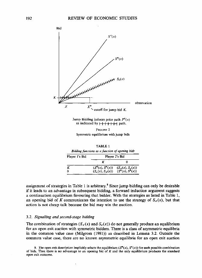
The choice of K to satisfy (2) implies that a bidder with an observation very close to 2 will be willing to open with a bid of K if that jump bid would induce his opponent to shift from a bidding strategy of S*(X) to &(X). Then, as shown in Figure 2, P“(y) represents the price path triggered by an unmatched jump bid, where y is the observation of the bidder who did not jump bid.

In the base model, the bidders make simultaneous choices of opening bids, each choosing between 0, an ordinary bid, and K, a jump bid. Table l summarizes the effect of these bids on future strategies in the second-stage. The choices (SA (X), &(X)) and K are fixed exogenously and assumed to be common knowledge between the players. The second-stage proceeds as an ordinary open exit (incremental bidding) auction in which jump bidding has no desirable effect and the players use bidding cutoffs as given in the table. If K is bid in the first-stage and one player’s subsequent strategy calls for a maximum bid below K, that player exits the auction immediately. Note that the importance of the open exit portion of the game is determined endogenously as a function of S, and K. For example, if S, is chosen to be a very passive strategy, then open exit bidding will tend to end quickly and have little influence on the final price.

The relationship between strategies and opening bids given in Table 1 ensures that there is an advantage to an unmatched bid of K in further bidding.’ However, the

6. For the case of common values, Levin and Harstad (1986) proved that this is the unique symmetric

7. Hendricks and Porter (1988) demonstrate some empirical evidence that a weakly positioned competitor equilibrium.

will bid relatively passively.

192

Bid

REVIEW OF ECONOMIC STUDIES

S A W

z X* ‘ cutoff for jump bid K .

Jump Bidding induces price path p ( x ) as indicated by path.

FIGURE 2 Symmetric equilibrium with jump bids

TABLE 1 Bidding functions as a function of opening b i d

Player l’s Bid Player 2’s Bid

K 0

assignment of strategies in Table 1 is arbitrary.* Since jump bidding can only be desirable if it leads to an advantage in subsequent bidding, a forward induction argument suggests a continuation equilibrium favouring that bidder. With the strategies as listed in Table 1, an opening bid of K communicates the intention to use the strategy of SA (X), but that action is not cheap talk because the bid may win the auction.

3.2. Signalling and second-stage bidding

The combination of strategies (SA (X) and S, (X)) do not generally produce an equilibrium for an open exit auction with symmetric bidders. There is a class of asymmetric equilibria in the common value case (Milgrom (1981)) as described in Lemma 3.2. Outside the common value case, there are no known asymmetric equilibria for an open exit auction

8. The open exit description implicitly selects the equilibrium (S*(x), S*(x)) for each possible combination of bids. Then there is no advantage to an opening bid of K and the only equilibrium produces the standard open exit outcome.


with two bidders (Bikhchandani and Riley (1992)).’ The information revealed in first-stage bidding can create an asymmetry between the

bidders, thereby justifying the choice of asymmetric strategies as second-stage equilibria for a particular class of jump bidding strategies. Note that the symmetric bidding strategies (S*(x), s*(x)) remain an equilibrium no matter what information is revealed in first-stage bidding.

Proposition 3.1. Suppose that it is common knowledge that xi > xi. Then the bidding strategies (SA (xi) , Sa(xj)) form an equilibrium for an open exit auction.

Proof. The player with the largest private observation wins the auction with symmetric bidding strategies. If Xi > X j then V J = V ( X j , X i ) 5 V(xI.9 X i ) SA ( X i ) . Similarly, Vi= v(x i , x j ) zv(x j , x j )>Sa(x j ) .

Given player i’s bidding strategy SA (x i ) , player j prefers to lose rather than to win the auction since v/ < SA(xi) . Given player j ’ s bidding strategy Sa (Xi), player i prefers to win rather than to lose the auction since Vi> S, (X,). Therefore, the bidding strategies (SA (xi) , S, (x i ) ) form an equilibrium given that X i > Xi. I I

Jump bidding will identify the player with the larger signal if the players use the same signalling strategy to determine their opening bids. Here, the term signalling strategy denotes any strategy which calls for a jump bid for private observations of at least a particular cutoff, X*. With signalling strategies, a jump bid is a credible signal of a favourable private observation. If one player opens with a bid of K and the other opens with a bid of 0, it must be that the jump bidder has the highest private observation (his observation must be at least X* and his opponent’s observation must be less than X*).

Pure private values and pure common values. The strategies SA (X) and Sa (X) take on special properties in the extreme cases of pure private values and pure common values. With pure private values, S, (X) <X requires the bidder to drop out at a price below his (known) true value. At the same time, once it is known that X i > Xi, player j also knows that he will lose the auction and expects a profit of zero from any strategy. Given any cost to continuing the bidding, any optimum strategy satisfies Sa (X) K-that is, a bidder with a signal below X* should drop out immediately upon seeing an opponent’s jump bid.

In the case of pure common values, there are asymmetric bidding equilibria of the symmetric open exit auction. It is then possible to choose pairs of strategies (SA (X), Sa (X))

which are bidding equilibria even without the information imparted by jump bids in the first-stage of competition.

Lemma 3.2. (Milgrom). L e t f (X) be any increasing, continuous positive-valued function, Then the strategy pair (SI (X), S2 (X)) where SI (X)= u(x,f (X)), S2 (X)= V(x, f - ’ (x)> is an equilibrium for a sccond-price common value auction.

These strategies are increasing and continuous because v and f are increasing and continuous functions. In equilibrium, bidding ties occur only for pairs of signals (U, z ) such that f (U) = z (implyingf-’(2) = U), thus satisfying the necessary condition derived by

9. Bikhchandani and Riley show that the symmetric equilibrium is the unique equilibrium for an open exit auction when U ( X , y ) > U( y , X) for X > y .


Bikhchandani (1986) : for S2 to be a best response to S1 , Sl(x) = S2 ( y ) only if S2 ( y ) = v(x , y ) . More importantly, this also implies that S1 (X) = v(x , y ) . Whenever the bidders tie in their bids, they must be indifferent between winning and losing after inverting their opponent's bidding function and then accounting for the information associated with that bid.

There are asymmetric equilibria with the additional property that S*(x) - Sa(x) is increasing under the further assumption that 2, and f2 are (strict) information complements with respect to v as defined by Bikhchandani and Huang (1989). That means that

Lemma 3.3. If X1 and X 2 are information complements, then there exist asymmetric equilibria ( S A (X), Sa (X)) for a second-price auction such that Sa(x) = v(x , f (X)) where f (X) < X is an increasing function and S*(x) - S a (X) is increasing.

Proof. By the earlier lemma, each choice off (X) produces an equilibrium. Consider the family of functions f (X) = x /n . As n increases, S a (X) approaches v(x, 0) because v is continuous. Since f l and f2 are information complements with respect to v, v(x , X) - v(x , 0) = S*(x) - v(x, 0) is increasing. Thus, for n sufficiently large, S*(x) - S a (X)

is increasing. I I

When the second-stage strategies (SA (X), S a (X)) are equilibria of the ordinary open exit auction, these strategies are fairly robust to first-stage bidding errors because they produce an equilibrium even without the information imparted by earlier jump bidding. See Section 5 for a full analysis of the effect of perturbations to bidding strategies and payoffs.

4. SYMMETRIC SIGNALLING EQUILIBRIA

This section proves the existence of a unique symmetric signalling equilibrium in the basic two stage game with K, S A , and Sa fixed. In this equilibrium, each player opens with a jump bid of K iff his private observation is above a given cutoff X*, where X* is determined as a function of ( K , S A , Sa).

With this symmetric jump bidding rule, the choice of second stage bid functions guarantees that the bidder with the highest private observation wins the auction. That is, the allocation of the object is identical to that from the symmetric equilibrium of an open exit auction (or to that for any first- or second-price auction in symmetric equilibrium), but the prices are not the same.

Figure 2 provides a preview of the properties of a symmetric equilibrium. At the lowest values of the lower observation y , a price given by symmetric bidding, S*( y ) is less than a price given by jump bidding, P"< y ) . Near the cutoff, X* for jump bidding, this inequality is reversed, as it must be, for otherwise there would be no benefit to jump bidding in equilibrium. As in the motivating example, X* is chosen to equalize the gains and losses from jump bidding conditional on receiving the signal X*. The first-stage of competition acts as a mini-first-price auction designed to distinguish situations where the bidders' evaluations of the object are close together from those in which they are not.


When one bidder has much more favourable information than the other, the players follow an equilibrium that favours that participant.

Theorem 4.1. Fix a three-tuple ( S A (X), S a ( X ) , K ) satisfying (2) and such that S a ( X ) < s*(x), S A (X) > S*(x), and S*(x) - Sa(x) is increasing in X. For this three-tuple, there exists a unique symmetric equilibrium of the metagame. In this equilibrium the player with the highest private observation wins the auction. The set of all possible three-tuples gives an infinite set of jump bid equilibria.

Proof. By Proposition 3.1, the second-stage bidding functions are best responses given signalling strategies in the first-stage, so it suffices to identify optimal first-stage signalling strategies.

Suppose that player i receives the private signal X and define

#(X, z ) = E [ S * ( X j ) - P K ( X j ) l X i = X , x ~ S Z ] . (4)

4 (X, z) measures the expected reduction in the price conditional on an unmatched jump bid by i assuming that (1) player j uses the value z as a cutoff for jump bidding and (2) player i wins the auction if X j l z , regardless of X and player i’s opening bid. These assumptions are purely for expositional purposes-note that they contrast with the standard outcome where player 1 wins the auction iff Xi > xi. When i wins the auction under these conditions a jump bid adjusts the price from S * ( X j ) to P K ( X j ) . 4(x, z) > 0 implies that jump bidding by i would be profitable in these circumstances when i’s observation is

The choice of Sa (X) requires that S*(x) - S a (X) is increasing, so s*(x) - PK(x) is also increasing and continuous. Therefore, 4 (X, z ) is continuous and strictly increasing in both arguments by the property of strict affiliation between X i and xi. Further, 4 (X, X) is negative for X near zero because K > s * ( O ) = 0 and positive for X large since K satisfies (2). By the intermediate value theorem, there is a unique value X* such that 4 (X*, X*) = 0.

This value X* provides the cutoff for jump bidding in the unique symmetric signalling equilibrium for (SA (X), S a ( X ) , K ) . Suppose that playerj bids K with signals of X* or above and 0 otherwise. To complete the proof, it remains to show that player i then wishes to use the cutoff of X* as well.

If player i receives a signal X >X*, 4 (X, X*) measures the expected reduction in the price from a jump bid if it is known that Xi< X*. Since X > X*, 4 (X, X*) > 0. Further, if i does not make a jump bid, i could lose an auction which he was slated to win if X, > X*

and Xj X i . Therefore, player i prefers to open with a bid of K for X > X*.

Now suppose that player i receives a signal X X* . If X, z x * , then player j bids K and wins the auction regardless of i’s bid since Xj > X i . When Xj < X*, i’s bid of zero implements the standard symmetric equilibrium of the open exit auction. Then if xi>x,, player i wins the auction with either bid, but he may also win in some cases if xi < Xj and he opens with K. The change in i’s profit from a jump bid as a function of xj is then

X.

The value ? ( X i ) represents the maximum signal for player j such that player i could change the outcome of the auction by jump bidding when xi<& The value ?(xi) is less


than X* since player j makes a jump bid with a signal of at least X* ; player i’s choice to jump bid with xi < X* can only affect the outcome of the auction if player j does not jump bid.

At the lowest values of xi, player i wins with either opening bid and H( , ) simply considers the difference in his winning price from jumping and bidding zero. In the midrange of values for xi (up to ? ( X i ) ) , i wins and pays P K ( X j ) , while he would lose and net zero profit from ordinary bidding. In this midrange, Xi x i , so that the expected value is

Therefore, player i’s profits from jump bidding for Xi< X* are less than 4 ( x i , J ( X i ) ) ,

and 4 ( X i , ? ( X i ) ) < O since xi<x* and ?(x i ) s x * . This demonstrates that player i prefers not to jump bid for x i < X * . I I

V ( x i , X , ) < v ( x j , x j ) = S * ( x j ) .

There may be other equilibria beyond those specified by the theorem. It may be possible to implement a signalling strategy equilibrium for some choices of & ( X ) where S*(x) - S, ( X ) is not always increasing. In addition, it is possible to relax the assumption that &(X) < S*(x), which assures that the weak bidding strategy is indeed weaker than the symmetric equilibrium strategy for each possible value of x.l0 There is still a unique signalling strategy equilibrium if S, ( X ) < S*(x) fails for the lowest values of X so long as equation (2) still holds. These additional equilibria do not expand the set of expected prices for the auction beyond those which can be produced from equilibria given by Theorem 4.1.

In many instances such as in takeover contests, jump bids will be sequential rather than simultaneous. The simultaneous jump bidding equilibrium corresponds to an analogous sequential jump bidding equilibrium with one change. If player 1 opens the game with a bid of 0, then player 2 has the choice of bids 0 and K, just as in the simultaneous game. But if player 1 opens with a jump bid to K, then player 2 must jump the bid in turn from K to v(x*, X*) in order to demonstrate a private observation of at least X * ; a bid by player 2 of K after player l’s jump bid is analogous to an initial bid of 0. Similarly, in the example with Ross Johnson and KKR bidding for RJR Nabisco, KKR had to raise Johnson’s bid from $75 to $90 (rather than just meeting the bid of $75) to make a credible signal of its seriousness given Johnson’s previous action.

Corollary 4.2. For each symmetric equilibrium of the base model (simultaneous) jump bidding game, there is an analogous equilibrium of the sequential move game with the same cutoflx* for jump bidding.

Proof. In the simultaneous bid game, neither player would wish to change her opening bid after the revelation of the other player’s action. Therefore, the simultaneity of their actions was not necessary for the derivation of the equilibrium, and the previous analysis carries over to the sequential game. I I

4.1. Revenue in jump bidding equilibria

The most important property of jump bidding equilibria is that these equilibria yield lower expected revenue than the symmetric equilibrium of an open exit auction.

10. It is also possible to relax the assumption that S,, (X) > S*(X), but this does not really expand the set of outcomes since the auction price depends on &(X) but does not d.epend on SA (X) directly.


Theorem 4.3. The symmetric equilibrium of the metagame provides an ex-ante Pareto improvement for the bidders over the symmetric equilibrium of an open exit auction.

Proof. The allocation from the metagame equilibrium is the same as that from the open exit auction in all cases and the price is identical in both cases if the players match opening bids. Otherwise, the opening bids indicate that one observation is above X* and that the other is below that cutoff. Then the same player wins in either auction, paying S*(y) in the open exit auction and PK( y ) in the English auction, where y <X* is his opponent’s private observation. Since the player with the higher observation wins in either auction, it is only necessary to compare expected prices of the auctions.

The proof of the theorem demonstrates that E( (S*(Xi) - PK( v) ) I X i = z, xi X*) = 0 at z= X* and is positive for z > X*. These cover the set of instances where there is a price difference in the two auctions so the open exit auction has a strictly higher expected price than the metagame English auction. I I

Strict affiliation of private observations is the driving force behind the reduction in expected revenue due to jump bidding. As shown in Figure 2, a bidder with a marginal observation of X* is indifferent between bidding 0 and K, for his gain in the second-stage from intimidating the opponent is negated by his loss from jumping immediately to K. One implication of affiliation is that as the private observation, xi increases from X*, the conditional distribution g(xj I Xi = X i ) favours values near X* increasingly relative to values near to zero. Jump bidding provides the greatest advantage to the winning bidder when the losing bidder’s private observation is close to X*, but less than X*. When a bidder with private observation X* is indifferent between jump bidding and not jump bidding, bidders with observations above X* will strictly prefer to jump bid because the conditional distribution puts increasing (relative) weight on observations where jump bidding is desirable. Thus, the shift in the conditional distribution of y as X increases from X* explains why jump bidding is desirable for bidders with signals above X*.

With independent observations, there remains a unique signalling equilibrium with jump bids for each three-tuple ( S , (X), S, (X), K ) , but the expected price for each jump bidding equilibrium would be equivalent to the expected price from an open exit auction. That result is an immediate implication of the revenue equivalence theorem. When the private signals are independent, the expected revenue is the same for all rules such that the bidder with the highest signal wins the auction in equilibrium. The following example illustrates this point.

Example 2. Suppose that Players i andj observe independent draws Xi and X, from a uniform distribution on (0, l), and bid for an object with value X i + X i . Then the symmetric equilibrium in an open exit auction consists of bid functions Si(Xi) = 2Xi ; S,(X,) = W,.

Take the degenerate equilibrium S, (X) = 2 ; S, ( X ) = 0 in which one player concedes the auction to the other to be the asymmetric equilibrium for the second-stage of the metagame. In the second-stage equilibrium, the weak bidder chooses a strictly dominated strategy for the original auction: namely, to drop out (bid zero). That strategy is not dominated in the metagame because it is implemented only when one’s opponent will win as a matter of course, and the jump bidding equilibrium is the unique symmetric outcome when there are bidding costs.

For any X, E(S”(Xj)IXj<X)=E(XjI X j < X ) = X . That is, for any choice of K < 1, the cutoff for a symmetric signalling equilibrium is X* = K. The players revert to symmetric


bidding in the second-stage unless exactly one of them bids K, in which case he wins the auction immediately. But then, without jumping, the same player would win the auction at expected price E(2X,I Xi < K ) = K . The expected price is the same in the metagame formulation as in the open exit (or second-price sealed bid) auction, yet the bidding history and realized prices are much different.

4.2. The informativeness of the price

In the symmetric equilibria of first- and second-price auctions, prices are determined by the order statistics of the private observations. The price alone reveals the highest observation, X('), in a first-price auction and the second highest one, d2), in a second-price auction. In either case, the price implies a bound for all of the remaining observations.

As a hybrid between first- and second-price rules, the dynamic auction modelled here obscures some of the information revealed in the price for other pricing rules. When a bid of K wins the auction, that price indicates X(') ?X*, d 2 ) gx* and d 2 ) 5 S i ' ( K ) , but does not pinpoint either observation exactly. The higher observation is the source of the price, K, but that price usually provides only diffuse information about the pair of private observations because of the pooled signalling strategies adopted by the players. On the other hand X(') z x * is more informative than X(') gd2) (as revealed in a second-price auction) for any value of d 2 ) 5 X*.

It is natural to associate the reduction in average price for the metagame from the open exit auction with a loss of information as revealed by the price. Yet, with an expanded set of strategies in the metagame, the price itself may reveal much of the bidding history. If K < &(X*), then a price above &(X*) requires both players to have jumped the bid in the first-stage, while a price below K reveals that neither player jumped. Example 3 illustrates the importance of this effect.

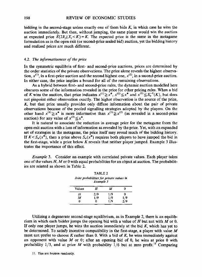
Example 3. Consider an example with correlated private values. Each player takes one of the values H, M or 0 with equal probabilities for an object at auction. The probabilities are related as shown in Table 2.

TABLE 2 Joint probabilities for private values in

Example 3

Values H M 0 H 2/9 1/9 0 M 1/9 1/9 1/9 0 0 1/9 2/9

Utilizing a degenerate second-stage equilibrium, as in Example 2, there is an equilibrium in which each bidder jumps the opening bid with a value of H but not with M or 0. If only one player jumps, he wins the auction immediately at the bid K, which has yet to be determined. To satisfy incentive compatibility in the first-stage, a player with value M must not prefer to choose K rather than 0. With a bid of K, he wins immediately against an opponent with value M or 0; after an opening bid of 0, he wins at price 0 with probability 1/3, and at price M with probability 1/6 but at zero profit." Comparing

11. Ties are broken randomly.


profits gives the condition K Z M / 2 for a player with value M to prefer not to jump in the first-stage. At K=M/2, the metagame gives identical payoffs for bidders of value M or 0 to those for the open exit auction. But a bidder of value H pays only K= M / 2 when he faces a bidder of value M in the metagame as opposed to M in the open exit auction. His overall average winning price is M / 2 + H/2 in the open exit auction and M / 4 + H / 2 in the metagame.

One interesting feature of the example is that the expected price is lower for the jump bidding equilibrium than for the open exit auction and yet the jump bidding equilibrium is strictly more informative than the open exit outcome. The addition of the jump bid K increases the set of possible prices to four as opposed to three in an ordinary open exit auction. As shown in Table 3, the price for the metagame yields a finer partition of states than the open exit equilibrium.

TABLE 3 Possible private values for each price in example 3

Price Value 1 Value 2 Open Exit Value 1 O.E. Value 2

The result of this example contrasts with the intuition that the revelation of additional information increases the expected price (see Theorem 15 of Milgrom and Weber ( 1982), which is also discussed in the Proof of Proposition 4.6 of this paper). That intuition is not relevant in jump bidding outcomes because the weak bidder may choose to ignore some of the information that is realized in equilibrium. After a successful jump bid in the example, the other bidder realizes that (on the equilibrium path) his opponent is willing to continue bidding up to her reservation value, H, but does not force the bidding to continue to H, the full information competitive price (this bidder will lose the auction in any case given that the jump bidder has a value of H ) . Thus, the price fails to reflect all of the information available to the bidders in equilibrium. Section 5 returns to the question of whether a losing bidder’s strategy of ignoring information revealed in prior bidding satisfies refinements of Nash equilibrium.

4.3. A folk theorem for multistage signalling

When the players match opening bids in the first-stage, the second stage game is simply a symmetric open exit auction with a reduced state space for private observations from that of the original auction. That leaves scope for further signalling as the new game retains the structure of the original one.

There are two natural ways to extend the set of jump bidding equilibria from a single stage of jump bidding. With ascending jump bids K1 < K2 . . . K,- 1 K,, the players can signal by jumping to the bid of K,,, in round m of jump bidding if both players jumped to each of K , , . . . , K,- previously. The signalling phase of the auction ends after the first-stage in which at least one player does not make a jump bid or if both players jump bid up to K,. At that point the players revert to the bidding strategies prescribed by Table 1 for an open exit auction. This description corresponds to a situation in which the auctioneer asks “Is anyone willing to bid Kl?” and continues to ask for bids of K2 and so on while he continues to get two positive responses.


With descending jump bids Kl > K2 . . . K,- > K,, both players have the opportunity to open with a bid of K, in round m of jump bidding if no one has bid prior to that. The signalling phase of the auction ends with the first jump bid or if no one bids in any of the n possible rounds of jump bidding. This description corresponds to a situation in which the auctioneer asks “Is anyone willing to bid K1?” and then reduces the price to K2 and beyond if no one opens the bidding at the given price.

Theorem 4.4. There are symmetric metagame equilibria with any number of stages of signalling based on ascending or descending jump bids. Each additional stage of signalling reduces the average price for the general auction and provides a Pareto improvement for the bidders.

Proof. See Appendix. I I

In the limit as the number of stages of jump bidding grows large (with jump bids spaced equidistantly between 0 and P), ascending and descending jump bids converge respectively to open exit and Dutch auctions.13 As the distance between jump bids becomes negligible for a long series of ascending jump bids, the metagame approximates a second- price auction; the price is determined by the point at which the losing bidder drops out of the jump bidding. The winner has jumped to a higher bid, but the difference in bids at that point is infinite~ima1.l~ Similarly, in the case of descending jump bids, the metagame approximates a Dutch auction, with the first bidder to jump the bid winning the auction. The implication of these results is that jump bidding can produce any expected revenue between that of the first-price (Dutch) auction and the second-price (open exit) auction.

Pr~positi~n 4.5. The equilibria of multistage games with descending signals cover the range of expectedprices between that of the first-price auction and the symmetric equilibrium of a second-price auction.

Proof. Fix a degenerate (or near degenerate with &(X) near to but not equal to 0) second-stage equilibrium. Next, consider the triangular sequence of descending jump bids

{ V/21

{ VP}, {2V/3, v/3) . . .

In the limit as n + m, the first and last entry in horizontal row n produce equilibria that approach the symmetric open exit and first-price equilibria respectively. Since each extra period of signalling reduces the expected price incrementally, this construction provides equilibria which cover the given range of expected prices. I I

It remains only to establish that the first-price and open exit auctions give tight bounds on expected prices for multistage jump bidding games, including games with combinations

12. The Pareto improvement is strict if the additional stage is nontrivial, and weak for each trivial stage. 13. These results are most obvious when the second-stage is degenerate so that a jump bid ends the auction. 14. Paradoxically, each additional opportunity to signal does reduce the price from the open exit auction,

but when the signals are infinitesimally apart from one another, the overall effect remains negligible.

AVERY JUMP BIDDING 20 1

or ascending and descending jump bids. Each opportunity to signal reduces the expected price, so the open exit auction gives the upper bound on expected price. An application of Milgrom and Weber’s comparison of general auction mechanisms demonstrates that the first-price auction gives a lower bound on expected price.

Proposition 4.6. Any multistage signalling equilibrium produces an expected price between that of a first-price and an open exit auction.

Proof. See Appendix. I I

4.4. Generalized one stage signalling

One goal of this paper is to demonstrate equilibria in sequential auctions where the participants choose the bids endogenously. That description is appropriate for the context of takeover bidding where there is no formal auctioneer. Suppose that bidders are allowed to choose their opening bids from any discrete set of options, (Kl, . . . , K,,), where K,, K,- 1 > K1 > 0. The players are implicitly allowed to choose an initial bid of zero by submitting no bid at all. Then there is an equilibrium of the game with a single stage of jump bidding which is equivalent to the equilibrium of a multistage signalling game with descending jump bids.

Theorem 4.7. Suppose that the bidders choose their opening bids endogenously and simultaneously from a fixed set of n possible bids and that they continue according to a prespecijied asymmetric equilibrium in favour of the higher bidder. Then there is a unique symmetric signalling equilibrium, with strategies identical to those strategies for an n-stage descending signal game with the same set of possible jump bids.

Notice that without the restriction that the higher bidder must be favoured in subsequent bidding, this game generates all of the multistage signalling equilibria endogenously. For example, if the only time that an asymmetric equilibrium is implemented is if one bidder opens with K and the other bids anything else, the equilibrium is identical to a one stage signalling game with only the jump bid K.

Proof. Consider the choice of the lowest possible jump bid K, in the one stage simultaneous game. In equilibrium, the only players who will not make at least that bid are those with the lowest signals. Suppose the cutoff for such a bid is 21. Then the choice to bid at least Kl is governed by a comparison between the expected price imposed by bidders with private signals in the range (0, 21). The expected price conditional on observation z > z l against bidders in that lowest range must be greater for jump bidding with z than for bidding 0, and must be identical for the two bids with z1. That condition is identical to the condition for the last cutoff in a descending sequence of the same n possible jump bids. Inductive reasoning based on this reasoning proves that the n-cutoffs for a symmetric equilibrium of the complicated one stage game must be the same as the cutoffs of the n-stage descending bid game, thereby producing an equilibrium. I I

5. PAYOFF AND STRATEGY PERTURBATIONS

Since the asymmetric bidding strategies for the second-stage rely heavily on the information conveyed by the bidding in the first-stage, it is natural to consider the effect of perturbations


to the payoffs and strategies of the players. Throughout this section, the term “aggressive bidder’’ refers to a player who has made an unmatched jump bid, and the term “weak bidder” refers to a player whose opponent has made an unmatched jump bid.

The asymmetric bidding functions of the second-stage have the odd property that the bidders appear to ignore the implications of their opponent’s opening bid. When Player i bids K and Player j bids 0 in the first-stage, these actions reveal that xi2 X* Z X j . With this new information, Player i knows that his maximum possible expected value for the object is V ( X i , X*) 5 v(xi , X i ) while Player j recognizes that his minimum expected value is

These results still seem to suggest that Player i should reduce and Player j increase their respective bids from the symmetric equilibrium functions for an open exit auction. Yet, their specified bidding functions call for them to do exactly the opposite. In the Nash equilibrium of Theorem 4.1, the second-stage bid functions are justified by the signals associated with earlier jump bids.I5 Given that play is on the equilibrium path, the players cannot increase their profits by adjusting their bids to accommodate the implication of the signals.

In equilibrium, there is a gap between the highest possible second-stage bid for a weak bidder, S, (X*), and the lowest possible second-stage bid for a strong bidder, S A (X*).

With the possibility of errors in bidding, it is natural for a weak bidder to consider bids in the range between these two bids. If it is profitable for the weak bidder to do so, then there is a reverberating effect of deviations by the weak bidder from &(X). Once weak bidders bid beyond &(X) in the second stage, there is less reason to jump bid in the first- stage and a jump bidding equilibrium may unravel.

This section returns to the base model (results for the multistage signalling outcomes are similar) and allows separately for small costs of bidding and small probabilities of bidding errors at either the first or the second-stage of bidding. An equilibrium will be called robust to a particular perturbation if the strategies for that equilibrium remain optimal in the limit when the probability of that perturbation is positive but arbitrarily small. A player subject to a strategy perturbation (i.e. a “bidding error”) is assumed to follow an exogenously given strategy without regard for whether that subsequent strategy is profitable.

The conclusion of this analysis is that jump bidding equilibria are robust to some, but not all perturbations. Bidding costs select extreme asymmetric bidding outcomes after an unmatched jump bid, when it becomes a unique best response for a weak bidder to drop out of bidding immediately at the price K. Without bidding costs, jump bidding equilibria are robust to first-stage bidding errors but not to second-stage bidding errors. The continuation strategies are equilibria because of the gap between the lowest possible bid for an aggressive bidder and the highest possible bid for a weak bidder in the second- stage after an unmatched jump bid. The inclusion of bidding errors may eliminate that gap and rule out continuation strategies (and overall jump bid outcomes) which were previously in equilibrium. If the continuation strategies are sufficiently extreme, then a bidding gap remains in the second stage even after an erroneous first-stage bid. Thus, a subclass of jump bidding equilibria are robust to first-stage errors. However, a second- stage bidding error eliminates any gap in bids for the continuation strategies. Therefore, jump bidding equilibria are not robust to second-stage bidding errors.

v ( x ~ , X*) 2 u ( x ~ , Xi).

15. There cannot be a signalling equilibrium where the weak bidder increases her subsequent bids in response to her opponent’s jump bid. Then, there is a disadvantage to jumping and first-stage signalling breaks down.


5. l. Bidding costs

If there is a cost for continuing in the bidding, then it is optimal for a bidder to drop out of an open exit auction as soon as he knows that he will lose the auction. Thus, the inclusion of even an arbitrarily small bidding cost (e.g. a flow cost per unit time in an open exit auction or a price per bid in a sequential bid auction) selects a degenerate equilibrium in the second-stage of bidding. In a symmetric signalling equilibrium, any unmatched jump bid must end the auction. Under these conditions, there remains a continuum of jump bidding equilibria selected from the previous set of equilibria.

Proposition 5.1. When the players use symmetric first-stage signalling strategies with a cut-ofl of X* in an auction with bidding costs, then any bidding strategies satisfying S A (X) S*(x*) and S, (X) < K form a second-stage equilibrium. For each ( S A ( X ) , &(X),

K ) of this form, there is a unique symmetric signalling equilibrium of the jump bidding game.’6

The implication of bidding costs is that it is a strict best response for the weak bidder to drop out rather than to continue bidding in the face of an unmatched jump bid. In the equilibria derived in Section 4, any bid function which loses the auction (including &(X),

S*(x) and all bidding functions between those two) is a best response for the weak bidder in the second-stage of the game. With a fixed and positive bidding cost, therefore, S, (X) < K remains a best response for the weak bidder to an unmatched jump bid even when there is a possibility of a bidding error by his rival in either stage of competition. As the probability of a bidding error tends to zero, the bidding cost outweighs any profit from further bidding which may accrue after an error by the strong bidder.

5.2. Bidding errors

If there is some possibility of an error by the aggressive bidder and there are no bidding costs, then it may be desirable for the weak bidder to compete beyond the level indicated by the function &(X). The profitability of further bidding by the weak bidder turns on the context of the auction and the type of error which is possible.

5.2.1. First-stage bidding errors. To isolate the effect of first-stage errors, suppose that there is a small probability that either player always (never) jumps the bid in the first-stage, regardless of his private observation. By assumption, such a player still follows the prescribed equilibrium in second-stage bidding. A bidder who deviates from the first- stage equilibrium is deemed to have “made an error”, since that player otherwise follows equilibrium play.

In the common value case, first-stage bidding errors cannot disrupt second-stage bidding if (SA (X), S, (X)) is chosen to be an asymmetric equilibrium of an open exit auction. Then the information from first-stage bidding is not necessary to support the combination of strategies (SA (X), &(X)) as an asymmetric equilibrium.

Propition 5.2. The symmetric signalling equilibrium is robust to first-stage errors for common value bidding when ( S A (X), S, (X)) is an equilibrium of an open exit auction.

16. Although there are many possible choices of (S, (X), & ( X ) ) , all equilibria for a given K produce the same allocation and price.


Proof. If the players match their opening bids but that bid was an error for one player, then the outcome is the same as in the original open exit equilibrium and neither player should deviate from S*(x) in second-stage bidding. The only exception occurs when one player makes a mistake by jumping to K with signal X such that z < v(x , X ) . Such an error has no effect since the final price is K whether that player errs or not.

Now consider the situation where player i jump bids but player j does not. Suppose that i considers the possibility that j made a mistake and that X,> X * . From i 's point of view, there is no difference between bidding up to U ( X i , X * ) or S A ( X i ) unless j made a mistake. On the equilibrium path, it is common knowledge that Xi < Xi and that j will drop out at a price below &(X* ) . Then player i wins with either cutoff point. If j continues to bid beyond & ( X * ) , i can conclude that j erred in his original bid and in fact, X, > X*. Given that information, it is rational for i to continue to bid up to SA ( X i ) while anticipating that j will continue until &(xi) v(x* , X * ) .

Now consider player j ' s perspective after an unmatched jump bid by i and that j is considering the possibility that i made a mistake with the jump bid and Xi < X * . So, player j might consider raising the bid from S, ( X i ) , perhaps to U ( X j , X * ) , which is the minimum expected value of the object if the players are on the equilibrium path. If i follows SA ( X i )

and j wins the auction by bidding to a value b > S, (Xi), then X i s Si1 (b) and xi< Si' (b) . In an asymmetric equilibrium, the players are indifferent between winning and losing when they tie in their bids. Thus, v (S i l (b ) , s,l(b)) = b and v ( x i , X,) b, meaning that j has lost money by winning the auction with a bid above S, (xi). I I

Outside of the common value case, jump bidding equilibria are iobust to first-stage errors so long as the asymmetric strategies to be played in the second-stage are sufficiently extreme. With the possibility of mistakes in first-stage bidding, a jump bidding equilibrium may call for a bidder with a lower private observation to win the auction. That is not of importance in the common value case because the object has the same value for both players. Otherwise, the object is worth more in expectation to the bidder with the higher private observation. In order to sustain a second-stage bidding equilibrium which may produce an inefficient allocation after a perturbation, the asymmetric bid functions must be quite distinct from the symmetric bid functions.

Proposition 5.3. Consider a jump bidding equilibrium where SA ( y ) > v(x* , y ) for each y , S, ( y ) v(x* , y ) for each y and also SA ( X * ) S, (X) and S A (0) > S, ( X * ) . This equilibrium is robust to Jirst-stage bidding errors.

Proof. Once again, if the players match their bids in the opening round, then they follow a symmetric bidding equilibrium in the second-stage; those bidding strategies are unaffected by the possibility of earlier errors.

If player i jumps the bid at the start of the game and player j does not, then player i stands to win the auction at a price of S, ( y ) . Suppose that player i considers a change in his bid from SA ( X i ) given the possibility of an error by player j in earlier bidding. When player j ' s private observation is y , the value to player i is U ( X i , y ) > S,( y ) . Since X i > X*

for i's (correct) jump bid, it is desirable for i to win the auction at the price S , ( y ) even if j made an error by not jump bidding. The assumption that S, (2) < SA ( X * ) guarantees that i will win the auction if j ' s opening bid was an error. Therefore, it remains optimal for player i to follow S A ( X i ) after an unmatched jump bid.

A similar analysis indicates that player j prefers not to win the auction after an unmatched jump bid by i even if i's jump bid was an error. The assumption that


SA (0) S, (X*) guarantees that i will win the auction after an unmatched jump bid even if i’s bid was an error. Therefore, it remains optimal for player j to follow S, (x i ) after an unmatched jump bid by i. I I

These conditions are sufficient but not necessary for the jump bidding equilibria to remain equilibria after first-stage perturbations; these are the conditions such that the aggressive bidder always wins every auction profitably after a first-stage perturbation. Note that the aggressive bidder may sometimes lose an auction after a first-stage bidding error by the weak bidder in the common value equilibrium.

The proof relies on the assumption that players revert to equilibrium strategies rather than so-called “best responses” after an error. For instance, a best response strategy would call for a player who failed to jump bid in the first-stage with a private observation of to bid up to v ( x , X*) in response to an unmatched jump bid. If bidders are restricted to such best responses after a bidding error, then jump bidding equilibria will only be robust to first-stage errors if the second-stage strategies call for weakly dominated strategies satisfying VA ( y ) >= U( l, y ) and V, ( y ) 5 v(0, y ) . Under these conditions, an aggressive bidder bids above his maximum possible value given his private observation and a weak bidder bids below his minimum possible value given his private observation.

5.2.2. Second-stage bidding errors. To isolate the effect of second-stage errors, suppose that there is a small probability that either player continues in second-stage bidding up to any exogenously given value in the range from 0 to v, regardless of his private observation and the earlier bidding.

Proposition 5.4. Jump bidding equilibria are not robust to second-stage errors.

Proof. After an unmatched jump bid by player i , it is common knowledge that X i 2 X* and Xj < X* since there is no possibility of a first stage error. Then, player j should continue bidding to at least .(Xi, X*) for K is at least U ( X j , X*) > S , ( X j ) and it is possible that player i will drop out (erroneously) prior to that price. Similarly, if the bidding continues to the price v(xi, X*), then player i should drop out. At that point, player j ’ s second-stage bid is out of equilibrium, and the price is more than the maximum possible value to player i given first-stage bidding. I I

6. CONCLUSIONS

English auctions are marked by discrete increases in bids. This paper demonstrates that participants can communicate within their competitive environment with their choice of bids, thereby coordinating their strategies to advantage. Each bidder would prefer a situation in which only she has the ability to signal, but this paper only considers symmetric games. The construction of each game is arbitrary in its choice of possible signals and subsequent asymmetric bidding functions. In practice, reputational effects could explain the selection of a particular signalling game structure. As bidders grow accustomed to competing with one another, they can develop their own set of expected bidding actions and corresponding interpretations of those bids. The parameters of the signalling game can be taken as proxies to describe these norms for a group of bidders.

The dynamic model of an English auction produces equilibrium outcomes with features of first- and second-price auctions. This result stands in stark contrast to standard theories which equate English and second-price auctions. In limiting cases, equilibria can


approach the form of pure first- or second-price auctions, and they cover exactly the range of prices between those two bounds. Bidding outcomes have the same properties for simultaneous and sequential games and are robust to a variety of plausible perturbations. In sum, these results suggest that jump bids in takeover contests and elsewhere are sug- gestive of keen strategies rather than irrational bravado.

APPENDIX 7.1. Calculations for Example 1

In the general framework of the motivating example, there are two bidders with private observations X and Y which are the sums A + B and B+ C respectively, bidding for a common value asset worth (X+ Y ) / 2 . A , B and C are independent U(0,l) random variables. Then the private observations have the joint density

if 1 s x s y ,

for X < y . The joint density is symmetric, so the density for pairs such that X hy is given by the identity f (X, y ) = f (U, X). The marginal density for a single observation is

X i f x l l , 2-X i fx> 1.

The conditional distributions for private observations are shown in Figure 3.

0 1 2

Marginal Density for Private Signal X

0 X 1 l+x 2 0 X - l 1 X 2

Conditional Distributions for Y given X < 1, X > l

FIGURE 3 Distributions for private observations


The private observations X and Y are correlated because they have the common term B. In the case where y 2 > y I > x z > x l > 1, however,

f(xI,yI>f(X2,Y2)=(2--Y2)(2-yI)=f(X2,YI)f(XI,Y2). (8)

Since strict affiliation requires LHS > RHS, only weak affiliation holds for X and Y. For that reason, the jump bidding equilibria for the example will not always reduce the expected revenue as shown in Section 5 for the case of strictly affiliated observations.

In a sealed bid first-price auction, the symmetric bidding equilibrium is given by B*’(x) = 2x/3, while in a sealed bid second-price auction, it is given by B*(x) =X. Expected revenue for the first-price auction is then

ERI = 2/3E(max (X, Y ) ) = 2/3E(B+max ( A , C)) = 2/3( 1/2 + 2 / 3 ) = 28/36. (9)

Expected revenue for the second-price auction is

ER2=E(min (X, Y))=E(B+min (A, C) )=(1 /2+ 1 /3 )=30 /36 . (10 )

One stage signalling. In the case of one stage binary signalling, the players can open with a bid of K or 0, where K is an arbitrary known value. If one player bids K and the other bids 0, then the auction ends immediately at the price K. The optimal cutoff X* for jumping to K in a symmetric equilibrium must satisfy the necessary (and sufficient) condition

E ( Y ( Y < x * , X = x * ) = K . ( 1 1 )

First consider values of K which induce X* 5 1 . The conditional distribution f ( y l y<x* , X = X*) = 2y/x*’. Then

K=E(YI Y<x* ,X=x*)= y*2y /x* ’dy=2x* /3 . JoX* (12)

That is, any choice K< 2/3 induces the cutoff X* = 3K/2 6 1. Note that the price is identical to that of the symmetric second-price sealed bid auction unless one observation is above X* and the other below that cutoff. In the jump bid auction, the price is then K, while in the sealed bid auction, it is the lesser of the two observations. That case occurs with probability

2P(X<X*, Y lx* )=2(P(X<x*) -P(X<x* , YSX*))

= 2 IoX* udu - 2 1; u(u/2 + (X* - u))du

= - 2x*3/3, ( 1 5)

yielding revenue 2 ( ~ * ) ~ / 3 -4(x*)*/9 for the jump bid auction. In contrast, the revenue for the same sets of observations is

2 6 ’ u f ( u ) P ( X ~ x * ) y = u ) d u (16)

= 2 JoX*uz(l -u/2-(x*-u))du (17)

= 2x*’- 5(x*‘/12) (18)

in the symmetric sealed bid second-price equilibrium. Comparing these two demonstrates that the signalling equilibrium gives revenue x*’/36 less than the expected revenue of the second-price auction for X* 6 1, or equivalently, K 1 2 / 3 . In this region, the choice K = 2/3, X* = 1 has the largest effect, reducing the expected revenue from sealed bid second-price value of 30/36 to 29/36.

For K > 2 / 3 , similar calculations apply, although they are much more complicated than those above. The relationship between K and X* is now K = ~ ( x * ’ + x * - 1)/3x*. Expected revenue takes the form of a fifth order polynomial taking a local minimum at X* = l , so that the choice K = 2/3 does indeed produce the lowest revenue from a one stage signalling game.

7.2. Proofs for Section 4

Proof of Theorem 4.4. Consider the cases of ascending and descending jump bids separately.


Ascending Jump B i h

Lemma 7.1. The addition of another possible stage of signalling with ascending jump bids and K,+ > K , does not affect the cutoffs in private observations for jump b i d at previous stages.

Proof. It follows by induction from the first-stage forward that the players will use signalling strategies at each stage, and that these are based on an increasing sequence of cutoffs X:, . . . , X,*. This is the appropriate order of stages for an inductive argument because then the cutoff at each stage is unaffected by the behaviour at future stages. At the margin X,, a further opportunity to signal has no effect; if both players jump to K,,, then a player with signal X,* is certain to lose. Similarly, the additional round of signalling has no effect on cutoffs for previous stages. 1 1

Given the lemma, the existence of a unique equilibrium in the multistage game with ascending jump bids follows from repeated iteration of Theorem 4.1 with only a single stage of signalling. This equilibrium is easy to describe because each cutoff X,* can be calculated as if stage m is the last stage of signalling. The earlier stages 1 through m - 1 affect the cutoffs for signalling in m through the manner in which they reduce the state space prior to stage m. Therefore, it is proper to calculate the cutoffs in ascending order.

Descending jump b i h

Lemma 7.2. The addition of an extra period of signalling based on descending jump bidr with K, , I < K , increases previous signalling cutoffs X; and provides a Pareto improvement for the bidders.

Proof. Let (X:, . . . , X,* ) and (X;, . . . , X; + ) be the signalling cutoffs corresponding to the set of jump bids ( K l , . . . , K,) and (K1, . . . , K,, ) and notice that these must be strictly decreasing sequences.

The addition of a final signalling stage with the jump bid K,, < K , encourages bidders to wait to jump bid at stage n, for they will now have another opportunity to distinguish themselves from bidders with lower private signals. Specifically, it increases the expected profits for a player, say i, with signal X,* (the cutoff when the n-th stage is the final stage of signalling) if he does not jump at stage n. If his opponent continues with the same cutoffs, including x*(n), then i's profits from jumping to K, are unchanged by the additional signalling stage and then he will prefer not to jump at stage n with signal X,*. Then the cutoff must increase to restore i 'S indifference in stage n. That is, X; > X,*, thereby increasing the profits for all those players with signals in the range between the cutoffs.

This adjustment has a reverberating effect in previous signalling stages. A bidder with a signal above X,*

achieves a strictly greater profit by signalling in stage n then in the original game. At the old marginal signal for stage n - 1, a bidder with signal X,*- I now prefers to wait to signal in period n, for he will then achieve higher profits against players with signals between X,* and X; than in the original signalling game. Therefore, X;- >X,* and the result follows by induction. I I

By backwards induction, there remains a unique symmetric signalling equilibrium for each stage of the multistage game with descending jump bids, and thus a unique symmetric equilibrium of the metagame with descending jump bids. This completes the proof of Theorem 4.4. I I

Discussion and Proof of Proposition 4.6. Let W"(X, z ) denote the conditional expected price for a bidder when he receives signal z , behaves as if he received signal X and wins the auction. M represents the fixed mechanism which determines the winner and the price he pays. Let W,! represent the partial derivative of W with respect to its i-th argument.

Lemma 7.3. (Milgrom and Weber)." Consider any incentive compatible mechanism in which the bidder with the highest observation wins the auction, losing bidders receive zero profit and W,"(x, z ) 0. Then the expected price in mechanism M is at least that of thejrst-price auction.

Milgrom and Weber argue that this property illustrates a general linkage principle; any dependence of the price on information affiliated with the highest private observation increases the expected price. Since the first- price rule relies on a minimal amount of information in setting the price as a function of the highest signal

17. This corresponds to Theorem 15 of their paper. They state a much less general result comparing the first- and second-price auctions, but their proof suffices for this result.


alone, it produces the least possible expected revenue.’* With multistage signalling and two bidders, second- price competition in the final incremental bidding stage serves to link the price to both private observations, thereby increasing the expected price beyond that of the first-price rule.

Proof of Proposition 4.6. It remains only to show that each signalling mechanism satisfies W ~ ( X , z ) 2 0. Let P(y ( ’ ) , yC2) ) denote the equilibrium price when one bidder has observation y(’) and the other ~ ( ~ ) 5 y ( ~ , . The first step is to show that P ( . , . ) is increasing in its second argument for mechanism M.

The signalling stages of mechanism M partition the space of private observations into intervals [0, z1 ), [zl, z2), . . . , [z,, m. Bidders with observations on the same interval behave identically through the signalling stages and then compete with each other using their ordinary second-price bidding functions in the final stage. When the bidders’ observations fall on different intervals, then the one with the higher signal wins in an asymmetric equilibrium after an unmatched jump bid.

Now consider a bidder with signal z on the interval [z,, z,+ His jump bidding actions induce a coarser partition of [0, z,) where a given jump separates him from an opponent with any observation on a particular interval. On each coarse interval, the price is of form max (Ki , S,,i(z)), where z is his opponent’s observation, and So,i is the weak bidding function corresponding to jump bid Ki. By definition, P( , ) is increasing in its second argument over each such interval, and is greater than S*( e ) at the left hand boundary while it is less than S*( * ) at the right hand boundary. Therefore, P( , ) takes a discontinuous jump at each boundary between coarse intervals, and it is increasing in its second argument in general. For Player 1, WM(x, z) = E[P(x, y)lX1 = z, y < X ] . Bidder 1 acts as though he has received signal X when in fact he has received z. Since P( , ) is increasing and XI and X 2 are affiliated, W M is increasing in its second argument and W,”(X, y ) 2 0 as desired. I I

Acknowledgements. I am particularly grateful to Bob Wilson, Sushi1 Bikhchandani, Jeremy Bulow, Pino Lopomo, Peter Zemsky, and Faruk Gul for their encouragement and many suggestions when this project was in its formative stages. I am also grateful to an anonymous referee for helping to generalize the results of the paper. Thanks also to Susan Athey, Judy Chevalier, Suzanne Cooper, Peter Cramton, Kent Daniel, Jim Hines, Paul Klemperer, Bob Marshall, Meg Meyer, Paul Milgrom, Jeroen Swinkels, Dimitri Vayanos, Richard Zeck- hauser and seminar participants for numerous helpful comments, and to Glena Ames for typesetting assistance. The author was supported by a National Science Foundation Graduate Fellowship and a State Farm Insurance Dissertation Fellowship.

REFERENCES BALDWIN, L. H., MARSHALL, R. C. and RICHARD, J.-F. (1997), “Bidder Collusion at Forest Service

BERNHARDT, D. and SCOONES, D. (1993), “Promotion Turnovers and Preemptive Wage Offers”, American

BHATTACHARYYA, S. (1988), “Preemptive Bidding with Private Valuations in Merger Games” (Mimeo,

BIKHCHANDANI, S. (1986), “Market Games with Few Traders” (Doctoral Dissertation, Stanford University). BIKHCHANDANI, S. and HUANG, C.-F. (1989), “Auctions with Resale Markets: An Exploratory Model

BIKHCHANDANI, S. and RILEY, J. (1991), “Equilibria in Open Common Value Auctions”, Journal of

BIKHCHANDANI, S . and RILEY, J. (1992), “Equilibrium in Open Auctions” (Mimeo, University of Califor-

CAMPBELL, C. (1997), “Coordination in Auctions with Entry” (Mimeo, Ohio State University). CRAMTON, P. (1994), “Money Out of Thin Air: The Nationwide Narrowband PCS Auction”, Journal of

Economics and Management Strategy, 4, 267-343. CRAMTON, P. (1997), “The FCC Spectrum Auctions: An Early Assessment”, Journal of Economics and

Management Strategy, 6, 431-495. CREMER, J. and McLEAN, R. (1988), “Full Extraction of the Surplus in Bayesian and Dominant Strategy

Auctions”, Econometrica, 53, 77-84. DANIEL, K. and HIRSHLEIFER, D. (1997), “A Theory of Costly Sequential Bidding” (Mimeo, University

of California, Los Angeles). DONALD, S. G. and PAARSCH, H. J. (1996), “Identification, Estimation, and Testing in Parametric Empirical

Models of Auctions within the Independent Private Values Paradigm”, Econometric Theory, 12, 517-567. FISHMAN, M. J. (1988), “A Theory of Preemptive Takeover Bidding”, Rand Journal of Economics, 19, 88-

101.

Timber Sales”, Journal of Political Economy, 105, 657-659.

Economic Review, 83, 771-792.

Harvard University).

of Treasury Bill Markets”, Review of Financial Studies, 2, 31 1-339.

Economic Theory, 53, 101 - 130.

nia, Los Angeles).

18. Riley (1989) offers an alternate explanation of the same result.


GLOSTEN, L. and MILGROM, P. (1985), “Bid, Ask and Transaction Prices in a Specialist Market with

HAILE, P. (1996), “Auctions with Resale Markets: An Application to U.S. Forest Service Timber Sales”

HENDRICKS, K. and PORTER, R. (1988), “An Empirical Study of an Auction with Asymmetric Information”,

HIRSHLEIFER, D. and PNG, I. (1990), “Facilitation of Competing Bids and the Price of a Takeover Target”,

KAMECKE, U. (1996), “Dominance or Maximin: How to Solve an English Auction’’ (Mimeo, Humboldt

LAFFONT, J.-J., OSSARD, H. and VUONG, Q. (1999, “Econometrics of First-Price Auctions”, Econometrica,

LAFFONT, J.-J. and VUONG, Q. (1996), “Structural Analysis of Auction Data”, American Economic Review,

LEVIN, D. and HARSTAD, R. (1 986), “Symmetric Bidding in Second-Price, Common-Value Auctions”, Econ-

LOPOMO, G. (1999, “Optimality and Robustness of the English Auction” (Stern School of Business Working

MASKIN, E. and RILEY, J. G. (1985), “Auction Theory and Private Values”, American Economic Review, 75,

McAFEE, P., McMILLAN, J. and RENY, P. J. (1989), “Extracting the Surplus in the Common-Value Auc-

MILGROM, P. (1981), “Rational Expectations, Information Acquisition, and Competitive Bidding”, Econome-

MILGROM, P. and WEBER, R. (1982), “A Theory of Auctions and Competitive Bidding”, Econometrica, 50,

MYERSON, R. (1981), “Optimal Auction Design”, Mathematics of Operations Research, 6, 58-73. PAARSCH, H. J. (1993), “Deriving an Estimate of the Optimal Auction: An Application to British Columbian

RILEY, J. G. and SAMUELSON, W. F. (1981), “Optimal Auctions”, American Economic Review, 71, 381-

RILEY, J. G. (1989), “Expected Revenue from Open and Sealed Bid Auctions”, Journal of Economic Perspec-

ROTHKOPF, M. and HARSTAD, R. (1991), “On the Role of Discrete Bid Levels in Oral Auctions”, European

Heterogeneously Informed Traders”, Journal of Financial Economics, 14, 71-100.

(Mimeo, University of Wisconsin-Madison).

American Economic Review, 78, 865-883.

Review of Financial Studies, 2, 587-606.

University).

63, 953-980.

86,414-420.

omic Letters, 20, 315-319.

Paper EC-95-03, New York University).

150-155.

tion”, Econometrica, 57, 145 1-1459.

trica, 49, 921-943.

1089- 1 122.

Timber Sales” (Mimeo, University of Western Ontario).

392.

tives, 3, 41-50.

Journal of Operational Research, 74, 572-58 1.

strategic jump bidding in english auctions jump...prices between those two bounds. these results...

Documents