strategic interaction finance 510: microeconomic analysis
TRANSCRIPT

Strategic Interaction
Finance 510: Microeconomic Analysis
Market Structures
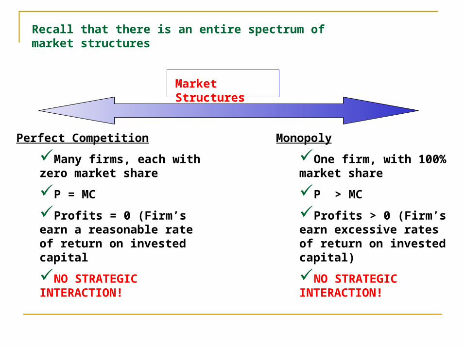
Recall that there is an entire spectrum of market structures
Perfect Competition
Many firms, each with zero market share
P = MC
Profits = 0 (Firm’s earn a reasonable rate of return on invested capital
NO STRATEGIC INTERACTION!
Monopoly
One firm, with 100% market share
P > MC
Profits > 0 (Firm’s earn excessive rates of return on invested capital)
NO STRATEGIC INTERACTION!

Most industries, however, don’t fit the assumptions of either perfect competition or monopoly. We call these industries oligopolies
Oligopoly
Relatively few firms, each with positive market share
STRATEGIC INTERACTION!
Wireless (2002)
Verizon: 30% Cingular: 22% AT&T: 20% Sprint PCS: 14% Nextel: 10% Voicestream: 6%
US Beer (2001)
Anheuser-Busch: 49% Miller: 20% Coors: 11% Pabst: 4% Heineken: 3%
Music Recording (2001)
Universal/Polygram: 23% Sony: 15% EMI: 13% Warner: 12% BMG: 8%

Further, these market shares are not constant over time!
9
11
14
15
20
21
Airlines (1992) Airlines (2002)
American
Northwest
Delta
United
Continental
US Air 7
9
11
15
17
19American
United
Delta
Northwest
Continental
SWest
While the absolute ordering didn’t change, all the airlines lost market share to Southwest.

Another trend is consolidation
44
55
677
888
9
Retail Gasoline (1992) Retail Gasoline (2001)
Shell
ExxonTexaco
Chevron
Amoco
Mobil
7
10
16
18
20
24Exxon/Mobil
Shell
BP/Amoco/Arco
Chev/Texaco
Conoco/PhillipsCitgoBP
Marathon
SunPhillips
Total/Fina/Elf

The key difference in oligopoly markets is that price/sales decisions can’t be made independently of your competitor’s decisions
Monopoly
PQQ Oligopoly
NPPPQQ ,..., 1
Your Price (-)
Your N Competitors Prices (+)
Oligopolistic markets rely crucially on the interactions between firms which is why we need game theory to analyze them!

The Airline Price Warsp
Q
$500
$220
60 180
Suppose that American and Delta face the given aggregate demand for flights to NYC and that the unit cost for the trip is $200. If they charge the same fare, they split the market
P = $500 P = $220
P = $500 $9,000
$9,000
$3,600
$0
P = $220 $0
$3,600
$1,800
$1,800
American
Del
taWhat will the equilibrium be?

Assume that Delta has the following beliefs about American’s Strategy
220$Pr
500$Pr
P
P
r
l
Probabilities of
choosing High or Low price
Player A’s best response will be his own set of probabilities to maximize expected utility
220$Pr
500$Pr
Pp
Pp
b
t
)1800($)3600($)0()9000($,
rlbrltpp
ppMaxbt
The Airline Price Wars

btbt
rlbltbt
pppp
pppp
211
)1800($)3600($000,9$),,(
Subject to
0
0
1
b
t
bt
p
p
pp Probabilities always have to sum to one
Both Prices have a chance of being chosen
)1800($)3600($)0()9000($,
rlbrltpp
ppMaxbt

First Order Necessary Conditions
09000 1 l 018003600 2 rl
01 bt pp
01 tp02 bp
02 01
0tp0bp
0
0
b
t
p
p
021
1
180036009000
lr
rll
4
3
4
1 rl
btbt
rlbltbt
pppp
pppp
211
)1800($)3600($000,9$),,(
4
3
4
1 rl pp
4
3
4
1 bt pp
0 1 rl pp 0 1 bt pp
1 0 rl pp 1 0 bt pp
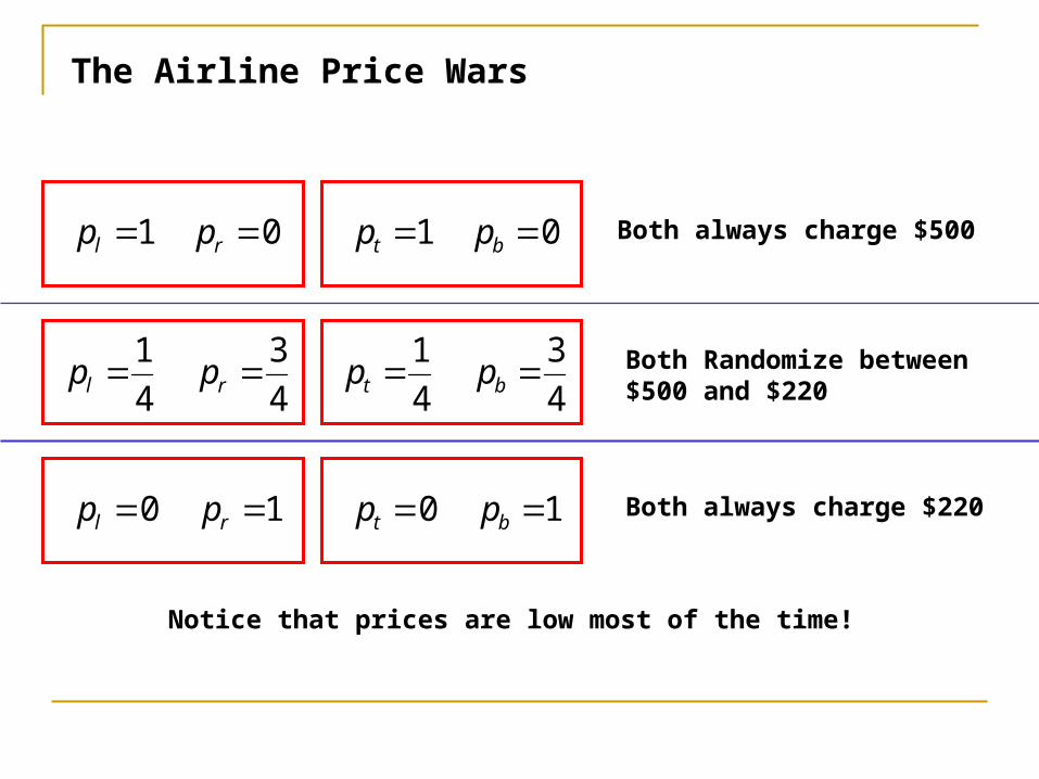
Both always charge $500
Both always charge $220
Both Randomize between $500 and $220
Notice that prices are low most of the time!
The Airline Price Wars

Continuous Choice Games – Cournot Competitionp
QD
There are two firms in an industry – both facing an aggregate (inverse) demand curve given by
BQAP
Aggregate Production
Both firms have constant marginal costs equal to $C

From firm one’s perspective, the demand curve is given by
1221 BqBqAqqBAP
Treated as a constant by Firm One
212 1BqqBqATR
Solving Firm One’s Profit Maximization…
cBqBqAMR 12 2
B
cBqAq
22
1

21 2
1
2q
B
cAq
In Game Theory Lingo, this is Firm One’s Best Response Function To Firm 2
1q
2q
B
cA
B
cA
2
Note that this is the optimal output for a monopolist!

Further, if Firm two produces
1q
2q
B
cA
B
cA
2
B
cA It drives price down to MC
BQAP
cB
cABAP

21 2
1
2q
B
cAq
The game is symmetric with respect to Firm two…
1q
2q
12 2
1
2q
B
cAq
B
cA
Firm 1
Firm 2
B
cA
2
B
cA
2
B
cA

1q
2q
Firm 1
Firm 2
*
1q
*2q
B
cAqq
3
1*2
*
1
B
cAqqQ
3
2*2
*
1
B
cA
B
cA
B
cA
3
2
2
1
Monopoly Output
Competitive Output
There exists a unique Nash equilibrium

A numerical example…
Suppose that the market demand for computer chips (Q is in millions) is given by
QP 20120
Intel and Cyrix are both competing in the market and have a marginal cost of $20.
Mqq CI 67.13
5
20
20120
3
1**
33.53$)33.3(20120 P

Had this market been serviced instead by a monopoly,
70$)5.2(20120
5.2*
P
MQ
20$
20120
MC
QP
1
1
MCp
4.15.2
70
20
1
Q
P
dP
dQ
4.11
1
20$70$

With competing duopolies
33.53$)67.1(206.86
67.1*
P
MQ
1
1
MCp
6.167.1
33.53
20
1
iQ
P
dP
dQ
6.11
1
20$33.53$
20$
206.862020120 112
MC
qqqP

One more point…
125$5.2)20$70($
70$
5.2*
P
MQ
55$67.1)2053($
33.53$
67.1*
P
MQ
Monopoly Duopoly
If both firms agreed to produce 1.25M chips (half the monopoly output), they could split the monopoly profits ($62.5 apiece). Why don’t these firms collude?

Suppose we increase the number of firms…
N
iiqBABQAP
1
Demand facing firm i is given by (MC = c)
iij j BqqBAP
iQ
iQB
cAq
2
1
21

ii QB
cAq
2
1
2
Firm i’s best response to its N-1 competitors is given by
ii qNQ )1( Further, we know that all firms produce the same level of output.
Solving for price and quantity, we get
BN
cAqi )1(
BN
cANQ
)1(
cN
N
N
AP
11

Expanding the number of firms in an oligopoly
BN
cAqi )1(
BN
cANQ
)1(
cN
N
N
AP
11
Note that as the number of firms increases:
Output approaches the perfectly competitive level of production
Price approaches marginal cost.
Lets go back to the previous example…

20$
20120
MC
QP
p
QD
$53
3.33
CS = (.5)(120 – 53)(3.33) = $112
$112
What would it be worth to consumers to add another firm to the industry?
56$
33.53$
33.32
67.1*
P
Mq
Recall, we had an aggregate demand for computer chips and a constant marginal cost of production.

20$
20120
MC
QP
p
QD
$45
3.75
CS = (.5)(120 – 45)(3.75) = $140
$140
31$
45$
75.33
25.1*
P
Mq
With three firms in the market…
A 25% increase in CS!!

0
1
2
3
4
5
6
Number of Firms
0
10
20
30
40
50
60
70
80
Firm Sales Industry Sales Price
Increasing Competition

Increasing Competition
0
50
100
150
200
250
300
Number of Firms
Consumer Surplus Firm Profit Industry Profit

20$
20120
MC
QP
Now, suppose that there were annual fixed costs equal to $10
How many firms can this industry support?
BN
cAqi )1(
c
N
N
N
AP
11
010$)20$( ii qP Solve for N

0
10
20
30
40
50
60
70
80
90
100
110
120
130
140
1 2 3 4 5 6 7 8 9 10 11 12 13 14 15 16 17 18 19 20 21 22 23 24 25
With a fixed cost of $10, this industry can support 7 Firms

21 2
1
2q
B
cAq
1q
2q
12 2
1
2q
B
cAq
Firm 1
Firm 2
The previous analysis was with identical firms.
*2q
*1q
Suppose Firm 2’s marginal costs are greater than Firm 1’s….

21
1 2
1
2q
B
cAq
1q
2q
12
12
2 2
1
2
cc
qB
cAq
Firm 1
Firm 2*2q
*1q
Suppose Firm 2’s marginal costs are greater than Firm 1’s….
Firm 2’s market share drops

B
ccAq
3
2 12*
1
B
ccAq
3
2 21*
2
B
ccAQ
3
2 21
+
As long as average industry costs are the same as the identical firm case
ccc
2
21
Industry output and price are unaffected!
Note, however, that production is undertaken in an inefficient manner!
With constant marginal costs, the firm with the lower cost should be supplying the entire market!!

Market Concentration and Profitibility
N
iiqBAP
1
Industry Demand
ii s
P
cP
000,10
H
P
cP
The Lerner index for Firm i is related to Firm i’s market share and the elasticity of industry demand
The Average Lerner index for the industry is related to the HHI and the elasticity of industry demand

The previous analysis (Cournot Competition) considered quantity as the strategic variable. Bertrand competition uses price as the strategic variable.
p
QD
Q*
P*
Should it matter?
BQAP Just as before, we have an industry demand curve and two competing duopolists – both with marginal cost equal to c.

1qD
BQAP
Bb
B
Aa
bPaQ
1
Cournot Case
1p
1qD
Bertrand Case
2BqA
1p
2p

Price competition creates a discontinuity in each firm’s demand curve – this, in turn creates a discontinuity in profits
2111
211
1
21
211
))((
2
)(
0
,
ppifbpacp
ppifbpa
cp
ppif
pp
As in the cournot case, we need to find firm one’s best response (i.e. profit maximizing response) to every possible price set by firm 2.

Firm One’s Best Response Function
mpp 2
Case #1: Firm 2 sets a price above the pure monopoly price:
2pc Case #3: Firm 2 sets a price below marginal cost
cppm 2
Case #2: Firm 2 sets a price between the monopoly price and marginal cost
mpp 1
21 pp
21 pp
2pc Case #4: Firm 2 sets a price equal to marginal cost
cpp 21
What’s the Nash equilibrium of this game?

Bertrand Equilibrium: It only takes two firm’s in the market to drive prices to marginal cost and profits to zero!
However, the Bertrand equilibrium makes some very restricting assumptions…
Firms are producing identical products (i.e. perfect substitutes)
Firms are not capacity constrained

An example…capacity constraints
Consider two theatres located side by side. Each theatre’s marginal cost is constant at $10. Both face an aggregate demand for movies equal to
PQ 60000,6 Each theatre has the capacity to handle 2,000 customers per day.
What will the equilibrium be in this case?

PQ 60000,6 If both firms set a price equal to $10 (Marginal cost), then market demand is 5,400 (well above total capacity = 2,000)
Note: The Bertrand Equilibrium (P = MC) relies on each firm having the ability to make a credible threat:
“If you set a price above marginal cost, I will undercut you and steal all your customers!”
33.33$
60000,6000,4
P
P
At a price of $33, market demand is 4,000 and both firms operate at capacity

Imperfect SubstitutesRecall our previous model that included travel time in the purchase price of a product
Firm 1Customer
x
txpp ~
Dollar Price
Distance to Store
Travel Costs
Length = 1
Consumers places a value V on the product

Imperfect Substitutes
Now, suppose that there are two competitors in the market – operating at the two sides of town
Firm 1Customer
x
Firm 2
x1
)1(~~21 xtpVtxpV
The “Marginal Consumer” is indifferent between the two competitors.
We can solve for the “location” of this customer to get a demand curve

Imperfect Substitutes
t
tppx
212
Firm 1Customer
x
Firm 2
x1
Nt
tppD
2
121 N
t
tppNxD
2
)1( 212

Both firms have a marginal cost equal to c
Nt
tppcp
2
)( 1211
Nt
tppcp
2
)( 2122
Each firm needs to choose price to maximize profits conditional on the other firm’s choice of price.
2
21
ctpp
2
12
ctpp

1p
2p
Firm 1
Firm 2
2
ct
2
ct
ct
ct
Bertrand Equilibrium with imperfect substitutes

Cournot vs Bertrand
1p
2pFirm 1
Firm 2
1q
2q
Firm 1
Firm 2
Suppose that Firm two‘s costs increase. What happens in each case?
Bertrand Cournot

Cournot vs Bertrand
Suppose that Firm two‘s costs increase. What happens in each case?
Cournot (Quantity Competition): Competition is very aggressive
Firm One responds to firm B’s cost increases by expanding production and increasing market share\
Best response strategies are strategic substitutes
Bertrand (Price Competition): Competition is very passive
Firm One responds to firm B’s cost increases by increasing price and maintaining market share
Best response strategies are strategic complements

Stackelberg leadership – Quantity Competition
In the previous example, firms made price/quantity decisions simultaneously. Suppose we relax that and allow one firm to choose first.
BQAP
Both firms have a marginal cost equal to c
Firm A chooses its output first
Firm B chooses its output second
Market Price is determined

Firm B has observed Firm A’s output decision and faces the residual demand curve:
BA BqBqAP
2BBA BqqBqATR
cBqBqAMR BA 2
ABA
B qqq
B
cAq
22

Knowing Firm B’s response, Firm A can now maximize its profits:
AB BqBqAP
22A
B
q
B
cAq
22ABqcA
P
22
2
ABqqcA
TR A
cBq
cAMR A
2
B
cAqA 2
Monopoly Output

B
cAqA 2
22A
B
q
B
cAq
B
cAqB 4
B
cAqq BA 4
3
B
cA
B
cA
B
cA
B
cA
4
3
3
2
2
1
Monopoly Output
Competitive Output
Cournot Output
Stackelberg Output
Essentially, Firm B acts as a monopoly in the “Secondary” market (i.e. after A has chosen). Firm B earns lower profits!

2
21
ctpp
2
12
ctpp
Sequential Bertrand Competition
With identical products, we get the same result as before (P = MC). However, lets reconsider the imperfect substitute case.
We already derived each firm’s best response functions
Now, suppose that Firm 1 gets to set its price first (taking into account firm 2’s response)
Nt
tppcp
2
)( 1211

Sequential Bertrand Competition
Nt
ptccp
4
3)( 1
11
Take the derivative and set equal to zero to maximize profits
2
31
tcp
4
5
21
2
tc
ctpp
Note that prices are higher than under the simultaneous move example!!

ND8
31
Sequential Bertrand Competition
2
31
tcp
4
5
21
2
tc
ctpp
ND8
52
Nt32
181 Nt
32
252
In the simultaneous move game, Firm A and B charged the same price, split the market, and earned equal profits. Here, there is a second mover advantage!!

Cournot vs Bertrand: Stackelberg Games
Cournot (Quantity Competition):
Firm One has a first mover advantage – it gains market share and earns higher profits. Firm B loses market share and earns lower profits
Total industry output increases (price decreases)
Bertrand (Price Competition):
Firm Two has a second mover advantage – it charges a lower price (relative to firm one), gains market share and increases profits.
Overall, production drops, prices rise, and both firms increase profits.
