stratal architecture in a prograding shoreface deposit

Old Dominion University Old Dominion University

ODU Digital Commons ODU Digital Commons

OES Theses and Dissertations Ocean & Earth Sciences

Spring 1999

Stratal Architecture in a Prograding Shoreface Deposit, Eastern Stratal Architecture in a Prograding Shoreface Deposit, Eastern

Shore, VA: Relationship to Grain Size, Permeability, and Facies Shore, VA: Relationship to Grain Size, Permeability, and Facies

Distribution Distribution

Andrew C. Miller Old Dominion University

Follow this and additional works at: https://digitalcommons.odu.edu/oeas_etds

Part of the Ocean Engineering Commons, and the Soil Science Commons

Recommended Citation Recommended Citation Miller, Andrew C.. "Stratal Architecture in a Prograding Shoreface Deposit, Eastern Shore, VA: Relationship to Grain Size, Permeability, and Facies Distribution" (1999). Doctor of Philosophy (PhD), Dissertation, Ocean & Earth Sciences, Old Dominion University, DOI: 10.25777/fgpa-9e17 https://digitalcommons.odu.edu/oeas_etds/64

This Dissertation is brought to you for free and open access by the Ocean & Earth Sciences at ODU Digital Commons. It has been accepted for inclusion in OES Theses and Dissertations by an authorized administrator of ODU Digital Commons. For more information, please contact [email protected].

https://digitalcommons.odu.edu/

https://digitalcommons.odu.edu/oeas_etds

https://digitalcommons.odu.edu/oeas

https://digitalcommons.odu.edu/oeas_etds?utm_source=digitalcommons.odu.edu%2Foeas_etds%2F64&utm_medium=PDF&utm_campaign=PDFCoverPages

http://network.bepress.com/hgg/discipline/302?utm_source=digitalcommons.odu.edu%2Foeas_etds%2F64&utm_medium=PDF&utm_campaign=PDFCoverPages

http://network.bepress.com/hgg/discipline/163?utm_source=digitalcommons.odu.edu%2Foeas_etds%2F64&utm_medium=PDF&utm_campaign=PDFCoverPages

https://digitalcommons.odu.edu/oeas_etds/64?utm_source=digitalcommons.odu.edu%2Foeas_etds%2F64&utm_medium=PDF&utm_campaign=PDFCoverPages

mailto:[email protected]

STRATAL ARCHITECTURE IN A PROGRADING SHOREFACE

DEPOSIT, EASTERN SHORE, VA: RELATIONSHIP TO GRAIN

SIZE, PERMEABILITY, AND FACIES DISTRIBUTION

by

Andrew C. Muller B.S., May 1989 Adelphi University

M.S., August 1992, Old Dominion University

A Dissertation Submitted to the Faculty of Old Dominion University in Partial Fulfillment of the

Requirement for the Degree of

DOCTOR OF PHILOSOPHY

OCEANOGRAPHY

OLD DOMINION UNIVERSITY May 1999

Approved by’

Donald J.P. Swift (Director)

Ronald E. Johnson (Member)

G. Richard Whittecar (Member)

Reproduced with permission of the copyright owner. Further reproduction prohibited without permission.

ABSTRACT

STRATAL ARCHITECTURE IN A PROGRADING SHOREFACE DEPOSIT, EASTERN SHORE, VA: RELATIONSHIP TO GRAIN SIZE,

PERMEABILITY, AND FACIES DISTRIBUTION

Andrew C. Muller Old Dominion University, 1999 Director Dr. Donald J.P. Swift

A fundamental concern of the stratigrapher is to develop predictive models of

stratigraphic organization. In sedimentology one o f the most significant problems that

has yet to be resolved is the fact that there is a lack of quantitative information

regarding the relationship between geometry of beds, thickness o f beds, grain size and

sedimentary structures in sandy environments, especially shallow marine deposits.

Scientists have also realized the need to correlate quantitative permeability to

sedimentary structures and scales of stratigraphic organization. The purpose of the

study is to investigate the scales of stratigraphic organization that control the variation

of grain size and permeability in shallow marine deposits. A model of stratal

architecture is constructed in order to relate scales of stratigraphic organization to these

properties. The hypothesis tested is that models o f stratal architecture are more

efficient predictors of grain size and permeability than are facies models in shallow

marine sands. Several methods are used to test the hypothesis, including mapping of

stratal geometry, measuring stratal characteristics, and the construction of facies

distribution through measured sections. These techniques are used to erect the stratal

architecture of strand plain deposits at Oyster, Virginia. ANOVA, Tukey-Kramer Means


Comparisons tests and variograms are performed to test the statistical significance of

mean grain size and permeability variability over multiple scales of stratigraphic

organization. Results from this study demonstrate that multiple levels of stratigraphic

organization are statistically significant with respect to the spatial variability o f grain

size and permeability, and that one-dimensional facies models are clearly unable to

resolve these important stratigraphic scales. The study also revealed that a parabolic

relationship exists between mean grain size and set thickness, and is thought to be the

evolutionary consequence of the progressive sorting process.


TABLE OF CONTENTS

Page

LIST OF TABLES......................................................................................................... viii

LIST OF FIGURES.......................................................................................................... xi

Chapter

L INTRODUCTION..............................................................................................1

GENERAL INTRODUCTION................................................................... 1Statement of the Problem................................................................ 1

Heterogeneity in Sedimentary Deposits................................1Numerical Models ofPhysical Heterogeneity....................... 3

GRANULOMETRIC PROPERTIES OF SEDIMENTS.............................. 4General.......................................................................................... 4Primary Properties..........................................................................5

Mineralogy and Fabric........................................................ 5Grain Size and Sorting........................................................ 6Shape and Roundness..........................................................8

Secondary Properties...................................................................... 9Porosity.............................................................................. 9Permeability......................................................................10Permeability and Grain Size...............................................11

LEVELS OF STRATIGRAPHIC ANALYSIS........................................... 14General.........................................................................................14Small Scale Architecture...............................................................15

GeneraL............................................................................ 15Small Scale Architecture: McKee and Weir (1953).............. 16Classification of Cross-Stratification..................................20

Mesoscale Architecture (Facies and Facies Models).......................26Vertical Architectural Patterns...........................................28Hierarchy of Bounding Surfaces........................................ 33

Large Scale Architecture (Depositional Sequences)....................... 35Architectural Classification used in this Study............................... 39

THE STUDY AREA............................................................................... 44General Geology of the Eastern Shore........................................... 44The Oyster Site as a Natural Lab................................................... 49Facies Erected in the Study Area................................................... 51


Chapter Page

HYPOTHESIS TO BE TESTED...............................................................52

THESIS LAYOUT................................................................................... 52

0. METHODS OF STUDY..................................................................................53

INTRODUCTION.................................................................................... 53Approach......................................................................................53Data Collected.............................................................................. 54

FIELD METHODS...................................................................................54Opening of Pit Faces..................................................................... 54Measured Sections........................................................................ 55Geological Mapping......................................................................55Sampling Procedures.....................................................................56

Grain Size......................................................................... 58Permeability......................................................................58Stratal Geometry Measurements.........................................58

LABORATORY METHODS....................................................................59Grain Size Analysis.......................................................................59Geostatistical Analysis.................................................................. 59

Textural Properties............................................................ 59Normalization of Textural Properties to Set Geometry. 60Variogram Construction.....................................................60Analysis of Variance (ANOVA).......................................... 61

ffl. ARCHITECTURE OF THE OYSTER SITE................................................... 67

INTRODUCTION.................................................................................... 67

FACIES ARCHITECTURE......................................................................67

STRATAL ARCHITECTURE.................................................................. 75General.........................................................................................75Coset A.........................................................................................77Coset B.........................................................................................80Coset C.........................................................................................87Coset D.........................................................................................89

VERTICAL PATTERNS..........................................................................94Set Thickness................................................................................94Grain Size.....................................................................................95


vi

Chapter Page

IV. GEOSTATISTICAL ANALYSIS OF THE OYSTER SITE...........................106

INTRODUCTION................................................................................... 106

STRATAL ARCHITECTURAL MAPS....................................................106Coset A........................................................................................ 107

Distribution of Grain Size Samples....................................107Distribution of Permeability Samples................................ 107

Coset B........................................................................................ 107Distribution of Grain Size Samples....................................I llDistribution of Permeability Samples................................ I l l

Coset C........................................................................................ 111Distribution of Grain Size Samples....................................111Distribution of Permeability Samples................................ 116

Coset D........................................................................................116Distribution of Grain Size Samples....................................117Distribution of Permeability Samples................................ 117

BIVARIATE STATISTICS......................................................................117General........................................................................................ 117Textural Properties....................................................................... 118

Mean Grain Size vs. Sorting..............................................118Mean Grain Size vs. Skewness.......................................... 118Mean Grain Size vs. Percent Gravel...................................120Sorting vs. Percent Gravel.................................................120Mean Grain Size vs. Permeability..................................... 120Sorting vs. Permeability.................................................... 123Mean Grain Size vs. Set Thickness....................................123

ANALYSIS OF VARIANCE RESULTS...................................................123General........................................................................................ 123Tukey-Kramer Means Comparison Test.......................................127Coset Variability...........................................................................128

Grain Size.........................................................................128Permeability..................................................................... 132

Set Variability...............................................................................136General.............................................................................136Coset A............................................................................ 137

Coset A: Grain Size Results...................................137Coset A: Permeability Results................................ 138

Coset B.............................................................................141Coset B: Grain Size Results....................................141Coset B: Permeability Results................................141


Chapter Page

Coset C........................................................................... 145Coset C: Grain Size Results....................................145Coset C: Permeability Results................................146

Coset D........................................................................... 146Coset D: Grain Size Results...................................146Coset D: Permeability Results................................149

VARIOGRAM RESULTS.......................................................................152General...................................................................................... 152Variogram Modeling....................................................................155Coset A....................................................................................... 155

Grain Size Results............................................................155Permeability Results........................................................ 156

Coset B....................................................................................... 156Grain Size Results............................................................156Permeability Results........................................................ 161

Coset C....................................................................................... 161Grain Size Results............................................................161Permeability Results........................................................ 167

V. CONCLUSIONS..........................................................................................171

INTRODUCTION.................................................................................. 171

SIGNIFICANCE OF THE OYSTER SITE ARCHITECTURALRESULTS...............................................................................................173

Facies Architecture...................................................................... 173Stratal Architecture...................................................................... 174Progressive Sorting on the Nassawadox Shoreface........................ 178

General............................................................................178Mean Grain Size vs. Set Thickness....................................184

SIGNIFICANCE OF ANOVA RESULTS................................................. 187

SIGNIFICANCE OF VARIOGRAM RESULTS....................................... 189

GENERAL CONCLUSIONS...................................................................189

FUTURE RESEARCH............................................................................190

BIBLIOGRAPHY..........................................................................................................192

VITA............................................................................................................................198


LIST OF TABLES

TABLE Page

1.1 Granulometric properties of sediments......................................................................5

1.2 Grain size classification scale (after Wentworth 1922)............................................... 7

1.3 Relative affects of primary granulometric properties onsecondary properties (after Pettijohn et al. 1986)....................................................... 15

1.4 Comparison of quantitative terms used to describe stratification(after McKee and Weir 1953).................................................................................. 20

1.5 Classification of cross-stratified units (after McKee and Weir 1953).........................21

1.6 Types of cross-stratification, grouped by lower bounding surface shape,grouping, scale and formation processes (after Allen 1984)....................................... 27

1.7 Comparison of stratigraphic organization terminology of the McKee andWeir system vs. Campbell’s terminology..................................................................27

1.8 Scales of stratigraphic organization used in this study...............................................44

2.1 Bata collected........................................................................................................ 54

3.1 Textural properties of each facies............................................................................74

3.2 Petrographic facies classification............................................................................ 75

3.3 Summary of average stratal geometry measurements of Coset A............................... 80

3.4 Textural properties of Coset A................................................................................ 83

3.5 Summary of the average stratal geometry measurements of Coset B......................... 83

3.6 Summary of textural properties for Coset B............................................................. 87

3.7 Summary of stratal geometry measurements for Coset C.......................................... 89

3.8 Textural properties of Coset C................................................................................ 91

3.9 Summary of stratal geometry measurements for Coset D..........................................94

3.10 Textural properties of Coset D................................................................................94


ix

TABLE Page

3.11 Results of significance tests for correlation between set positionand mean grain size................................................................................................101

4.1 Coset A: grain size set statistics.............................................................................. 109

4.2 Permeability set statistics: Coset A..........................................................................110

4.3 Coset B: grain size set statistics...............................................................................114

4.4 Permeability set statistics: Coset B..........................................................................115

4.5 Coset C: grain size set statistics.............................................................................. 116

4.6 Permeability set statistics: Coset C..........................................................................116

4.7 Coset D: grain size set statistics.............................................................................. 117

4.8 Permeability set statistics: Coset D......................................................................... 117

4.9 ANOVA results for grain size of cosets.................................................................... 130

4.10 Means comparison results of cosets: grain size........................................................ 132

4.11 ANOVA results for permeability of cosets................................................................136

4.12 Means comparison test for permeability of cosets.................................................... 136

4.13 ANOVA results of grain size for Coset A................................................................. 138

4.14 Grain size means comparisons results: Coset A........................................................140

4.15 ANOVA results for set permeability: Coset A...........................................................140

4.16 Means comparison results for permeability. Coset A................................................142

4.17 ANOVA results for grain size: Coset B.................................................................... 144

4.18 Means comparison results for grain size: Coset B.....................................................144

4.19 ANOVA results of permeability. Coset B................................................................. 145

4.20 Means comparison results of permeability Coset B................................................. 148


X

TABLE Page

4.21 ANOVA results of grain size: Coset C......................................................................149

4.22 Means comparison results of grain size: Coset C......................................................149

4.23 ANOVA results of permeability: Coset C................................................ 149

4.24 Means comparison results of permeability for Coset C.............................................151

4.25 ANOVA results of grain size: Coset D......................................................................151

4.26 Means comparison test results o f grain size: Coset D............................................... 151

4.27 ANOVA results of permeability: Coset D................................................................. 151

4.28 Means comparison test results o f permeability: Coset D...........................................152

4.29 Number ofdata pairs for horizontal variogram: Coset A, grain size.......................... 159

4.30 Number of data pairs for vertical variogram: Coset A, grain size..............................160

4.31 Number of data pairs for horizontal variogram: Coset A, permeability..................... 160

4.32 Number of data pairs for vertical variogram: Coset A, permeability..........................161

4.33 Number of data pairs for horizontal variogram: Coset B, grain size.......................... 164

4.34 Number of data pairs for vertical variogram: Coset B, grain size.............................. 165

4.35 Number of data pairs for horizontal variogram: Coset B, permeability......................165

4.36 Number of data pairs for vertical variogram: Coset B, permeability..........................166

4.37 Number of data pairs for horizontal variogram: Coset C, grain size.......................... 166

4.38 Number of data pairs for vertical variogram: Coset C, grain size.............................. 167

4.39 Number of data pairs for horizontal variogram: Coset C, permeability..................... 170

4.40 Number of data pairs for vertical variogram: Coset C, permeability..........................170


LIST OF FIGURES

FIGURE Page

1.1 Permeability trends in a cross-bedded sand, showingthe influences of sedimentary structure on fluid flow (after Pryor 1973)..................... 13

1.2 Sub-aqueous bedforms produced as a result of increasingstream power and grain diameter (after Allen 1963).................................................. 17

1.3 Diagram illustrating the terminology used to definestratification (after Allen 1984).................................................................................19

1.4 Diagram illustrating the classification of cross-stratification(after McKee and Weir 1953)...................................................................................22

1.5 Diagram illustrating cross-strata set scale, setgrouping, base relationship (after Allen 1963,1984)................................................. 24

1.6 Classification of cross-strata shape and lower bounding surfaceshape (after Allen 1963,1984)..................................................................................25

1.7 The complete turbidite (after Walker 1984)............................................................. 30

1.8 Vertical patterns of stratification and their relatedgrain size patterns (after Allen 1984)........................................................................31

1.9 Hierarchy of bounding surfaces (after Brookfield 1977)........................................... 34

1.10 Six fold hierarchy of bounding surfaces for fluvial deposits.A to E represents successive enlargements of fluvial unit showing the rank of bounding surfaces indicated by the circlednumbers (after Miall 1985).......................................................................................36

1.11 Fluvial architectural elements (after Miall 1985)...................................................... 37

1.12 Features of a sequence and it’s associated system tracts, boundaries within systems traces are parasequences.HST is high stand systems tract, LST is low stand system tract,TST is transgressive systems tract, SB1 is type 1 sequenceboundary and mfs is maximum flooding surface (after Vail 1987)....................................40

1.13 Stratigraphic consequences o f eustatic sea level changes(after Vail etal. 1979)..............................................................................................41


xii

FIGURE Page

1.14 The Eastern Shore of Virginia, showing the positions of theAccomack and Butlers BlufFMembers.................................................................... 45

1.15 Cross section showing the stratigraphic relationship of the membersof the Nassawadox Formation (after Mixon 1985).................................................... 48

1.16 Evolution of the Nassawadox Spit..........................................................................50

2.1 Sample grid used to place samples on the outcrop face.............................................57

2.2 Definition sketch for a normative set and the normalization ofsamples to set geometry.......................................................................................... 62

2.3 Definition sketch of a typical variogram..................................................................63

3.1 Photograph of trough cross-stratification at the Oyster Site. Note thebasal gravel lags in cross strata sets (arrows)............................................................ 68

3.2 Photograph illustrating sediments from the lower Butlers BluffMember................................................................................................................. 68

3.3 Facies distribution between easting 958 and 964 (after Parsons 1998).......................70

3.4 Facies distribution between easting 964 and 970(after Parsons 1998)................................................................................................ 71

3.5 Facies distribution between easting 970 and 976(after Parsons 1998)................................................................................................ 72

3.6 Facies distribution between easting 976 and 982(after Parsons 1998)................................................................................................73

3.7 Percentage of facies within the Butlers BIuffMember.............................................. 76

3.8 Petrographic facies vs. classical facies.....................................................................76

3.9 Mesoscale architecture of the Oyster Site................................................................ 78

3.10 Photomosaic of Coset A......................................................................................... 79

3.11 Histogram of lamina thickness for Coset A.............................................................. 81

3.12 Histogram of lamina width for Coset A....................................................................81


xiii

FIGURE Page

3.13 Histogram of set thickness for Coset A......................................................................82

3.14 Histogram of set width for Coset A........................................................................... 82

3.15 Photograph of the stratal geometry of Coset B...........................................................84

3.16 Histogram of lamina thickness for Coset B............................................................... 85

3.17 Histogram of lamina width for Coset B..................................................................... 85

3.18 Histogram of set thickness for Coset B......................................................................86

3.19 Histogram of set width for Coset B........................................................................... 86

3.20 Photomosaic of Coset C, illustrating parallel laminations andset breaks................................................................................................................ 88

3.21 Histogram of set thickness for Coset C......................................................................90

3.22 Histogram of set width for Coset C........................................................................... 90

3.23 Photograph illustrating the break between Cosets C and D,and the general characteristics of Coset D................................................................. 92

3.24 Histogram of set thickness for Coset D......................................................................93

3.25 Histogram of set width for Coset D...........................................................................93

3.26 Vertical pattern of set thickness for easting 964.........................................................96




3.30 Vertical pattern of set thickness for easting 972....................................................... 100

3.31 Vertical distribution of mean grain size for easting 965.3......................................... 102

3.32 Vertical distribution of mean grain size for easting 966............................................ 103

3.33 Vertical distribution of mean grain size for easting 968............................................104


xiv

FIGURE Page

3.34 Elevation vs. mean grain size................................................................................. 105

4.1 Stratal architecture of the Oyster Site: Coset A....................................................... 108

4.2 Stratal architecture of the Oyster Site: Coset B and C............................................. 112

4.3 Stratal architecture of the Oyster Site: Coset C and D............................................. 113

4.4 Mean grain size vs. sorting.....................................................................................119

4.5 Mean grain size vs. skewness................................................................................. 121

4.6 Mean grain size vs. % gravel..................................................................................121

4.7 Sorting vs. % graveL..............................................................................................122

4.8 Mean grain size vs. permeability............................................................................ 122

4.9 Sorting vs. permeability......................................................................................... 124

4.10 Mean grain size vs. set thickness............................................................................ 124

4.11 Example of box plots used in this study(after JMP Statistical Guide 1995).......................................................................... 126

4.12 Definition sketch of means comparison circles(after JMP Statistical Guide 1995).......................................................................... 129

4.13 Coset box plots for grain size, and means comparison circle plot............................ 131

4.14 Example of the normal quantile plot(after JMP Statistical Guide 1995).......................................................................... 133

4.15 Q-Q plot Coset A...................................................................................................133

4.16 Q-Q plot Coset B...................................................................................................134

4.17 Q-Q plot Coset C...................................................................................................134

4.18 Q-Q plot Coset D.................................................................................................. 135

4.19 Coset box plots and means comparison circles of permeability................................ 135


XV

FIGURE Page

4.20 Box plots and means comparison circles of grain size: Coset A............................... 139

4.21 Box plots and means comparison circle for permeability: Coset A...........................139

4.22 Box plots and means comparison circles of grain size: Coset B............................... 143

4.23 Box plots and means comparison circles of permeability: Coset B...........................143

4.24 Box plots and means comparison circles of grain size: Coset C............................... 147

4.25 Box plots and means comparison circles of permeability: Coset C...........................147

4.26 Box plots and means comparison circles of grain size: Coset D............................... 150

4.27 Box plots and means comparison circles of permeability: Coset D...........................150

4.28 Definition sketch of parameters used to construct the directionalvariogram (after Pannatier 1996)............................................................................154

4.29 Horizontal variogram of grain size: Coset A........................................................... 157

4.30 Vertical variogram of grain size: Coset A............................................................... 157

4.31 Horizontal variogram of permeability: Coset A......................................................158

4.32 Vertical variogram of permeability: Coset A......................................................... 158

4.33 Horizontal variogram of grain size: Coset B.......................................................... 162

4.34 Vertical variogram of grain size: Coset B.............................................................. 162

4.35 Horizontal variogram of permeability: Coset B......................................................163

4.36 Vertical variogram of permeability: Coset B..........................................................163

4.37 Horizontal variogram of grain size: Coset C.......................................................... 168

4.38 Vertical variogram of grain size: Coset C............................................................... 168

4.39 Horizontal variogram of permeability: Coset C.......................................................169

4.40 Vertical variogram of permeability: Coset C...........................................................169


xvi

FIGURE Page

5.1 The formation of cross strata sets, notice the scourformed in front of the migrating dune.................................................................... 176

5.2 The progressive sorting mechanism acting throughtime steps T1-T3 (after Swift et al. 1991a)............................................................. 180

5.3 Textures and structures of depositional systems thathave undergone progressive sorting (after Swift et al. 1991b)....................................182

5.4 Progressive sorting on the Nassawadox shoreface.................................................. 183

5.5 Hjulstrom curve, relating grain size to velocity(after Seibold and Berger 1982).............................................................................186


1

CHAPTER I

INTRODUCTION

GENERAL INTRODUCTION

Statement of the Problem

The construction of predictive models o f stratigraphic organization is a

fundamental concern of the stratigrapher. Pettijohn and colleagues (1973) have pointed

out that one of the most important unresolved problems in sedimentology is that there is

a lack of detailed information on the geometry, thickness of beds, grain size, and

sedimentary structures in sandy environments. Another significant problem in

sedimentology is that there is an extraordinary lack of quantitative permeability data

correlated to sedimentary structures and stratigraphic organization (Chandler et al.

1989; Davis et aL 1993; Doyle and Sweet 1995). Furthermore, there is a continual need

to incorporate detailed sedimentological data into predictive models of stratigraphic

organization.

Heterogeneity in Sedimentary Deposits. Scientists have realized that sediments

and sedimentary structures are generally not homogeneous or uniformly random in

nature. Sedimentary deposits typically display multiple layers of contrasting grain size

and permeability at discrete or continuous scales. These layers may range from

millimeters to tens of meters thick and are often geometrically anisotropic and

discontinuous (Allen 1963; Cushman 1990). Therefore, a hierarchy of sedimentary

bodies can be erected over a range of spatial scales and used to describe the

The journal model used for this dissertation was the Journal of Sedimentary Research.


2

heterogeneity in sedimentary deposits. The term “architecture” is used to describe the

two and three dimensional study of the geometry o f individual sediment bodies, and their

stratigraphic organization (Allen and Allen 1990). Studies of stratigraphic architecture

have focused almost exclusively on mesoscale and large scale architecture, and have only

been conducted in aeolian or fluvial deposits (Brookfield 1977; Miall 1985; Miall 1988;

Davis et al. 1993; Cowan 1991; Jordan and Pryor 1992). Small scale architecture

(centimeter scale) o f marine deposits have been almost entirely ignored. I believe that in

order to develop predictive models of stratigraphic organization that relates prim ary

properties such as bed structure and grain size to secondary properties of permeability

and porosity, we need to understand how small scale heterogeneity fits into a

classification of large scale heterogeneity at the basin scale. Only then can we fully

describe the true heterogeneity of a deposit. I propose to investigate the architectural

controls of permeability, grain size and facies distribution in shallow marine deposits.

Stratigraphers have been constructing qualitative models of sedim entary

architecture over the past several decades; however the development of more powerful

computational techniques have made it possible to incorporate detailed sedim entary

characteristics into simulations of fluid flow. Therefore there is a need for detailed

quantitative information on sedimentary structures over several spatial scales.

Hydrologists have led the way in applying geo statistical techniques to granular properties

of sediments, but have often overlooked the stratigraphic order at larger spatial scales.

Geologists have been constructing architectural models on large spatial scales often

times missing the importance of small scale organization. It is essential to bridge the gap

between the large scale studies of geologists and the smaller scale studies of hydrologists


3

(Walker 1984; Leeder 1982; Chandler et aL 1989; Davis et aL 1993,1997; Doyle and

Sweet 1995).

Numerical Models o f Physical Heterogeneity. The characteristics of petroleum

reservoirs, such as permeability, porosity and grain size have become vital components

to petroleum production, as have the characteristics o f ground water aquifers for water

resources and pollutant transport. Field studies of Freyberg, 1986, Garabedian et aL

1991, and Davis et aL 1993, have all shown that geological heterogeneity is the dominant

control on the migration and dispersion of ground water contaminant plumes. Other

studies have been successful in showing that enhanced oil recovery is mainly dependent

on the detailed characterization of reservoir properties over a range of spatial scales

(Lake and Carroll 1986; Lake et al. 1991). Numerical models that use governing

equations to solve subsurface fluid flow usually require maps of spatially variable

hydraulic properties. In most studies, the complete three-dimensional structure of

hydraulic properties as well as the geologic structures have not been measured.

Therefore, modelers have incorporated numerous methods to interpolate between the

data points obtained. Koltermann and Gorelick (1996) recognize three basic image

creation techniques in order to get a complete picture of the heterogeneity of an aquifer.

The first group of techniques are structure imitating methods. These methods utilize a

number of techniques including probabilistic rules, correlated random fields and

deterministic constraints based on facies recognized. Structure imitating techniques also

include sedimentation pattern matching and spatial statistical algorithms. The second

group o f techniques are defined as process imitating methods, and include various

calibration methods for the aquifer model as well as geological process models. The


4

third group of techniques are known as descriptive methods. Descriptive methods

attempt to define zones of hydraulic properties within an aquifer by coupling geologic

observations with one dimensional facies models. The current transport models in use

today do an inadequate job of predicting the small scale heterogeneities that control

pollutant dispersal in aquifers (Cushman 1990; Hess et aL 1992). Therefore, accurate

descriptions of the local geometry o f sub-units must be conducted because they are

essential in defining flow field boundaries and preferential pathways of solute transport.

Koltermann and Gorelick (1996) have pointed out that models that incorporate three

dimensional surface flow fields, and hybrid methods that can utilize all of the available

geologic, geophysical and hydrological information are missing from the literature.

Determining how the architecture o f a deposit controls the spatial distribution of

permeability and grain size is an important basic sedimentological problem that will

enhance future modeling efforts for amplified oil recovery and solute transport problems

that currently dominate environmental problems of today and most likely the next

century. Quantification of the stratal architectural controls of aquifer properties will give

solute transport modelers the ability to incorporate “reaT’ sedimentary structures into

their models which will significantly increase the predictive ability of these models.

Modeling solutions that contain this detailed type of sedimentological information wifi be

invaluable to scientists and managers who need to make difficult decisions regarding

various environmental problems.

GRANULOMETRIC PROPERTIES OF SEDIMENTS

General

Sedimentologists are primarily interested in the processes that transport and


deposit sediments. As a consequence the sedimentologist often uses granulometric

properties of the sedimentary body in order to infer how the deposits were formed.

Granulometric properties of a sedimentary deposit are also known as the texture of the

sediment, and may be divided into two general categories, primary characteristics and

secondary characteristics. Primary granulometric properties o f sands are the mineralogy,

grain size, sorting, shape of particles, roundness, surface texture, and the fabric.

Secondary properties are properties o f the sedimentary body that are dependent upon the

fundamental properties listed above. These properties include porosity, permeability,

saturation and the bulk density (Table 1.1), (Pettijohn et aL 1987; Berg 1986; Miall

1990).

Table 1.1.- Granulometric properties o f sediments

Primary Secondary

mineralogy porositygrain size permeabilitysorting saturationshape bulk density

roundness surface texture

fabric

Primary Properties

Mineralogy and Fabric. Terrigenous sands are commonly composed of quartz,

feldspars and rock fragments. The matrix which is the finer grained material between the

grains in sandstones typically comprises clay minerals such as kaofinite, Qlite and

montmorillonite. Quartz is the dominant mineral o f most sands and sandstones because

it is the most resistant to both chemical and physical weathering. The cementing material


6

that holds the sandstone together is commonly a precipitated overgrowth of silica,

carbonate or iron oxides during early or late stage diagenesis (Folk 1974; Pettijohn et aL

1987; Berg 1986).

Grain Size and Sorting. Grain size and sorting are the most frequently

measured granulometric properties o f sands and sandstones, and are used to infer the

transporting agent, the strength o f the transporting agent, and the conditions under

which the deposits were formed. It can also be used to deduce the sediment transport

direction, and for these reasons it is no wonder that there is a tremendous body of

literature on the techniques and interpretations o f grain size analysis. Several methods

are currently used to measure grain size, and include sieving, pipetting, sediment tubes,

microscopy as well as Electrozone and laser particle counters. Geologists classify

particle sizes according to the standardized scheme o f Wentworth. Table 1.2 illustrates

the Wentworth scale. Grain size is commonly reported using the phi (<J>) transformation.

The grain size diameter in phi units is equal to the negative log base 2 of the diameter in

millimeters. Sieving is the most common method for granulometric analysis for fine

sands up through gravels. Pipette analysis is widely used for silts and clays, and for

sandstones, thm section microscopy is the only method accepted. Sedimentation tube

methods gained popularity in the late 1970's and throughout the 1980's because o f the

smaller sample sizes required, the speed of the analysis and the idea that settling velocity

is an important hydraulic property o f the sediment as compared to the sieve method.

Recently, the pharmaceutical industry and engineers have led the way in particle size

characterization with new developments in Electrozone and laser diffraction particle

analyzers. These methods are beginning to gain acceptance in the sedimentological


7

Table 1.2.- Grain size classification scale (after Wentworth 1922)

Diameter Diameter Class Sediment Rock

(mm) <piri) Names Name

256 -8 Boulders

64 -6 Cobbles Gravel Conglomerate

4 -2 Pebbles

2 -1 Granules

I 0 Very Coarse

05 1 Coarse

0.25 2 Medium Sand Sandstone

0.125 3 Fine

0.062 4 Very Fine

0.031 5 Coarse

0.015 6 Medium sot Siltstone

0.007 7 Fine

0.004 8 Very Fine

<0.004 < 8 Clay Clay Claysrone

community (Folk 1974; Lewis 1984; Anderson and Kurtz 1979; Gibbs 1974; Middleton

1976). Statistical measurements that are derived from granulometric analysis include

sorting, skewness and the kurtosis. Many attempts have been made by researchers to

use these statistical parameters in discriminating between different depositional

environments. These measurements may be estimated using graphical techniques or they

may be calculated as moment measurements. Sorting is the measure o f the dispersion

around the central tendency, and is therefore the standard deviation o f the grain size

distribution. Sorting is considered an important textural property because it is used as an


8

indication o f the energy level within the depositional environment. Sediments that are

classified as well sorted are those in which two-thirds of the grain size falls within less

than one Wentworth grade. Moderately sorted sediments contain sizes that range

between one and two Wentworth grades, and poorly sorted sediments range over more

than two Wentworth grades. Beach and dune sediments are typically the best sorted,

while the poorest sorting tends to be in glacial tills and mudflows. Skewness and

kurtosis are the least important of the statistically derived properties from granulometric

analysis. Skewness refers to the degree o f asymmetry, and ranges from positive values

for a finely skewed sediment to negative values for a coarsely skewed deposit. The

kurtosis is a measure o f the peakedness o f the curve, (Folk and Ward 1957; Folk 1973;

Lewis 1984; Friedman 1961; Visher 1969; Shepard and Young 1961; Middleton 1976).

Shape and Roundness. Shape and roundness are important because they

contain information about the modification of grains due to abrasion, chemical

weathering and sorting. They may also be important in provenance problems. Shape is

defined by varying ratios of a particles three axis, and is expressed as sphericity.

Sphericity is defined as the degree to which the three axis of a particle have equal

dimensions. Roundness refers to the curvature of the comers of the grains. Visual

estimates o f sphericity and roundness are often used in sedimentological studies, but do

not receive nearly as much attention as grain size or sorting. Surface texture is studied

with the aid of a binocular or polarizing microscope, and more recently the scanning

electron microscope. Studies on surface texture often reveal a variety o f microstructures

such as fracture patterns and striations which may give clues to the transporting agent

(Folk 1973; Lewis 1984; Pettijohn et aL 1987).


The fabric of the sediment body refers to the spatial arrangement and orientation

of the grains that make up the sediment body, and is dependent on the transporting

agent, grain size, shape and roundness. There have not been many studies on grain

fabric because of the difficulty in quantifying this property (Folk 1974; Pettijohn et aL

1987).

Secondary Properties

Porosity. Porosity is defined as the percent of void space that occurs between or

within the individual grains o f a sediment body. Porosity can be classified into four

general types, intergranular, intragranular, fracture and solution porosity. Intergranular

porosity is defined as the percent o f voids between individual grains. Intragranular

porosity is the percentage o f voids within the grains. Fracture porosity may be micro or

macro and solution porosity is a result of the solution of the cementing material.

Solution porosity is commonly known as secondary porosity. Total porosity is simply

the measure of all of the void spaces whereas effective porosity is a measure of just the

interconnected void spaces. Effective porosity is usually measured instead of total

porosity because it a more meaningful measurement for the flow of fluids. Porosity is

typically measured in the laboratory and expressed as percent o f bulk volume.

P=(Vp/Vb)lQO=(Vb-Vm)lOO/Vb

In equation 1-1, P is the porosity, Vb is the bulk volume, Vp is the pore space volume

and Vm is the mineral volume (Berg 1986; Pettijohn et aL 1972; Fetter 1988).

Studies have shown that for natural sediments, porosity is a function of grain


10

size, sorting, shape, fabric and the amount of cementing material. The packing of

sedimentary grains contributes significantly to the fabric o f the sand body, and is

believed to be the most important factor controlling porosity. Cubic packing has the

loosest arrangement o f grains, and therefore the highest porosity. At the other end of

the spectrum is rhombohedral packing which has the tightest arrangement and therefore

theoretically the lowest porosity (Morrow et aL 1969; Rodgers and Head 1961; Thickell

and Hiatt 1938; Fraser 1935).

Permeability. The capacity of a sediment body to transmit a fluid is known as

the permeability. Permeability is dependent upon the connected voids within the

sediment body, and many researchers believe that it is also a function of grain size,

shape, sorting and porosity. In Darcy’s (1856) classic paper, he showed that the rate of

flow through a porous medium such as sand is directly proportional to the head loss and

inversely proportional to the length of the sand column.

Q --K A{hl -h2)/L (1'2)

Q in equation 1-2 is the volume rate of flow, K is known as the constant of

proportionality, A is the cross sectional area and the difference between the heights of

the water (hi and 2) is the head loss. Permeability is usually expressed in terms of

volume flux, and equation 1-3 can be written in the more familiar form known as Darcy’s

Law.

V-Q/A - -K(dh/dL) ( l' 3)


11

K is known as the constant o f proportionality or hydraulic conductivity, V is the volume

flux and dh/dL is the head loss per unit length in the above equation. The Darcy is

the unit of choice for hydrogeologists and engineers and is defined as:

In this definition, Q/A is the flow volume per unit area, p. is the viscosity, dL/dp is the

pressure gradient and the last part is a conversion factor (Fetter 1988; Berg 1986; Fraser

1935). It is important to distinguish permeability from hydraulic conductivity.

Permeability is an intrinsic property of a porous medium. Unlike hydraulic conductivity

it does not depend on the properties of the particular fluid. Hydraulic conductivity does

depend on the fluid properties. Therefore the hydraulic conductivity is specific to the

particular fluid and takes into account the density and viscosity of the fluid at standard

temperature and pressure. Typical unites for hydraulic conductivity are meters/day.

Permeability and Grain Size. There have been numerous attempts to correlate

permeability to grain size over the past several decades and several empirical equations

have been developed by both engineers and geologists. The reasoning behind the

attempts to correlate grain size and permeability stems from studies that have shown that

have shown a fourfold increase in pore throat area occurs when there is a doubling in

the diameter of particles (Fraser 1935). This realization has lead to the very familiar

empirical relationship used to calculate hydraulic conductivity from grain size.

Darcy=(Q/A)(\x)(dL/dp){ 1.0133.H 06) (1-4)

K=cd2 (1-5)


12

K is the hydraulic conductivity, d is the diameter of the particles and c is a dimensionless

constant. Krumbein and Monk (1943) developed an empirical equation that relates grain

size and sorting to permeability.

K = cd2e ,33° (1-6)

The diameter in equation 1-6 is measured as the geometric mean diameter, c is a constant

and a is the sorting (Russel and Shepherd 1990; Pettijohn et aL 1986; Potter and Mast

1962; Mast and Potter 1962).

In a widely cited study by Beard and Weyl (1973), artificial mixtures of sands

were used to relate permeability and porosity to grain size and sorting. They concluded

that permeability decreased with decreasing grain size and that porosity increased with

sorting. Pryor (1973) took 922 samples of porosity and permeability from various

depositional environments including river bars, dune and beach environments and related

them to grain size, sorting and sedimentary structure. The results indicated that

permeability increased with sorting, and porosity increased with grain size for river bar

sands only. Also, the results suggest that there are greater variations of grain size and

permeability within bedding than between, and that depositional processes have a strong

affect on porosity and permeability distributions (Fig. 1.1).

Byers and Stephens (1983) conducted a statistical analysis of hydraulic

conductivity and particle size in a fluvial sand. They concluded that the strongest

correlation between hydraulic conductivity and grain size is that o f the log of hydraulic

conductivity and the effective grain size d,0 (10% finer particle size).


13

Permeability Boundary

Fig. 1.1.- Permeability trends in a cross-bedded sand, showing the influences of sedimentary structure on fluid flow (after Pryor 1973).


14

They also suggest that grain size and hydraulic conductivity contain different spatial

correlation structures in the vertical plane. According to Byers and Stephens, the grain

size pattern is more structured than hydraulic conductivity and follows the observed

stratigraphy. However, the hydraulic conductivity was best modeled as a simple random

variable. Several problems exist with this study. First, when comparing the geometric

mean grain size and effective grain size, coefficients of correlation (R2) are not reported;

however when calculated they reveal no significant difference between them. This means

that it does not matter whether one uses effective grain size or mean grain size, they are

both equally poor in predicting permeability from empirical equations. Also, a hierarchy

o f sedimentary structures was not used to interpret the hydraulic conductivity structure.

Recently, Panda and Lake (1995) attempted to improve permeability predictions by

incorporating the entire particle size distribution. Table 1.3 shows the relative effects

primary granulometric properties have on secondary properties. Although several

studies have been conducted on this subject, clearly there is a need for more work in this

field.

LEVELS OF STRATIGRAPHIC ANALYSIS

General

As stated earlier, one of the primary objectives of the stratigrapher is to describe

and interpret the three dimensional nature of stratigraphic organization o f the

sedimentary basin fill, which is referred to as the architecture o f the sedimentary body.

Small scale to mesoscale architecture is largely a function o f subsidence, sea level and

the sedimentary dynamic processes that govern the formation o f depositional

environments and depositional systems.


15

Table 1.3.- Relative affects o f primary granulometric properties on secondary properties (after Pettijohn et al. 1986)

Primary Properties Secondary Properties

grain size Permeability decreases with grain size, porosity maybeunchanged, or may decrease

sorting As sorting gets poorer, permeability and porosity decrease

fabric Permeability and porosity decrease with tighter packing,permeability may follow bedding structures

cement permeability and porosity decrease with increasing cement

At this level of stratigraphic organization, sedimentary properties are measured on scales

o f millimeters to tens of meters. Meso scale to large scale architecture usually involves

the sub-disciplines of lithostatigraphy, chrostratigraphy and biostratigraphy. The

principal objective on the large scale is the reconstruction of major depositional

sequences, and often employ the use of seismic sections and the application of sequence

stratigraphic concepts (Miall 1990; Walker 1984; Leeder 1982).

Small Scale Architecture

General. For several decades sedimentologists have known that sandstones may

be sub-divided into genetically related strata by an hierarchically ordered set of bedding

contacts (Allen 1963). Strata may be horizontally deposited, or they may be formed as

cross strata. Cross strata are defined as being compositionally or texturally distinct layers

that are more or less steeply inclined to the principal bedding axis. Most cross strata are

due to the movement of ripples and dunes. Strata that are horizontally or consist of low

angle parallel lamina have bedding planes that are flat. Flat or parallel bedding usually

occurs in medium to fine grained sand, and may be rich in mica. Lamina in flat beds are


often only a few grain diameters thick making it difficult to measure individual lamina

thicknesses. In medium to fine grained sands and sandstones that have relatively little

mica, parallel or horizontal laminations are indicative of upper flow regime conditions.

Parallel laminations may also form under lower flow regime conditions if the critical

velocity for ripple formation has not been reached. Fig. 1.2 illustrates the resultant sub

aqueous bedforms with varying grain diameter and stream power (Allen 1964,1970;

Jopling 1962; McBride et aL 1975; Bridge 1978; Co Hinson and Thompson 1982). The

first detailed account of cross bedding was conducted by HaH (1843), who used the term

“diagonal bedding”. Sorby (1859), showed that cross strata could arise from Gilbert-

type delta building through flume experiments. He called this type of bedding “drift

bedding”. Sorby also described a smaller scale o f cross strata that he called ripple drift,

and showed that these structures formed as result of net deposition occurring with

current ripple migration.

Small Scale Architecture: McKee and Weir (1953). McKee and Weir's (1953)

classification of stratification and cross stratification is the first attempt to categorize

stratigraphic organization, and starts by recognizing three basic groups o f terms that

should be applied to sedimentary deposits. The first group contains qualitative terms

such as stratum and cross stratum. These terms emphasize the attitude and relation of

rock units without any implication of scale. The second group refers to quantitative

terms that are related to the thickness of stratification. These terms include thick-

bedded, thin-bedded and laminated- The third basic group also relates to quantitative

terms, however, this group is concerned with the thickness of splitting within stratified

units. These terms include massive, slabby and flaggy.


Stre

am

Pow

er

( erg

s/cm

A2

/sec

)

17

20,000

10,000

g,0006,000

4.000

2.000

1,000

400

200

1008060

40

Plane Bed

RipplesCross-Lamina

Upper Flow Regime

Lower Flow Regime

DunesCross-Bedding

Plane Bed

No Sediment Movement

Jm X X.01 .02 .03 .04 .OS .06 .07 .08 .09 .1

D(cm )

Fig. 1.2.- Sub-aqueous bedforms produced as a result o f increasing stream power and grain diameter (after Allen 1963).


18

These three groups o f terms are a good way to begin describing the nature of stratified

sedimentary rocks.

Stratification is the first term to be described in the qualitative term group. This

term is used to describe layering in sedimentary deposits. A stratum is defined as the

basic unit or single layer of homogenous or gradational Iithology, and a scale is not

implied. McKee and Weir (1953) point out that this term is not synonymous with the

terms of bed or lamina because these terms imply a scale. Cross stratification refers to

layers deposited at one or more angles to the dip of the formation. A group of strata

that are genetically related constitutes a set. Strata within a set are separated by erosional

surfaces, or by an abrupt change in character such as Iithology. A group o f two or more

sets is designated as a coset, a group that is composed of strata and cross-strata is

known as a composite set. This is a large sedimentary unit that has a constant or

gradational Iithology (Fig. 1.3), (McKee and Weir 1953). The quantitative terms are

important because they imply a scale to be used. The term bed is reserved for any

sedimentary stratum that is greater than 1 cm. thick. Lamina refers to stratum that are 1

cm. or less in thickness. Therefore, a cross-bedded deposit is a single unit containing

homogeneous or gradational Iithology deposited at an angle to the original dip and

greater than 1 cm thick (Table 1.4). This classification sets up specific limits for the

terms thick-bedded and thin-bedded. Table 1.4 also shows the relationship of the

splitting properties.

McKee and Weir (1953) also proposed a general classification for cross stratified

units based on seven criteria. The criteria used are: (1) The character of the lower

bounding surface, (2) The shape of the cross strata set, (3) The cross strata set axis


19

Fig. 1.3.- Diagram illustrating the terminology used to define stratification (after Allen 1984).


20

Table 1.4.- Comparison o f quantitative terms used to describe stratification (afterMcKee and Weir 1953)

Stratification Cross Thickness SplittingTerms Stratification Property

Terms TermsVery thick- Very thickly cross bedded cross beds Greater than 120

cm.Massive

Thick-bedded Thickly cross bedded 120 cm to 60 cm Blocky

Thin-bedded Thinly cross bedded 60 cm to 5 cm. Slabby

Very thin- bedded

Very thinly cross bedded 5 cm to 1 cm Flaggy

f jmnmfwj cross laminated Cross lamina 1 cm to 2 mm. Shaiy (sthstooe) Platy (sandstone)

Thinly-laminated

Thinly cross laminated 2 mm or less Papery

attitude, (4) Axis symmetry of the cross strata, (5) The arching of the cross strata, (6)

Cross strata dip and (7) Individual cross strata length (Table 1.5). From these seven

criteria, three major types of cross-stratification can be recognized (Fig. 1.4). Type 1 is

referred to as a simple set of cross strata. This deposit is called a simple set because the

lower bounding surface is a surface of non deposition instead of an erosional surface. A

simple set is formed by deposition alone. A planar set o f cross strata makes up the

second type of cross-stratification, and has a lower bounding surface which is a planar

surface o f erosion. This deposit is formed from beveling and subsequent deposition.

The third type of cross-stratification is call a trough set. This deposit results from

channeling and subsequent deposition. In this classification system, the basic criterion

that determines the type of cross strata is the nature o f the lower bounding surface.

Classification o f Cross-Stratification. Allen (1963) proposed a descriptive

classification for cross-stratified sediments based on six elements that are similar to the


21

McKee and Weir classification. Allen made a refinement to this classification in order to

incorporate all of the known kinds of structures. A second goal of this paper was to give

possible origins for the known types o f cross-stratification.

Table 1.5. - Classification o f cross-stratified units (after McKee and Weir 1953)

Primary Secondary Attributes

AttributesBounding Set shape Axis Cross-strata Cross-strata Cross- Cross-strata Cross-

surface of cross- attitude of symmetry arching strata dip length strata

strata set cross-strata type

Nonerosional Lenticular Plunging Symmetric Concave High angle Small scale Simple

surfaces (>20

degrees)

(< 1 foot)

Planar surfaces Tabular Noo- Asymmetric Straight Medium Planar

of erosion pfunging scale

(I to 20 feet)

Curved surfaces Wedge- Convex Low angle Large scale Trough

of erosion shaped (<20

degrees)

(> 20 feet)

Allen's basic criticism ofMcKee and Weir’s (1953) work was that it did not include

cross-stratification associated with small scale ripple marks or the possibility that some

sets or cosets may occur as solitary units. Allen recognized that some sets occur alone

with deposits of different structures. Solitary sets are fundamentally different from a

group o f genetically related cross-stratified sets.

Solitary sets in marine deposits have been interpreted to form as the result o f the

construction of isolated shallow banks.


22

Simple cross-stratification The lower bounding surfaces of Sets are non-erosional surfaces.

Planar cross-stratificationThe lower bounding surfaces ofSets are planar surfaces of erosion.

Trough cross-stratification The lower bounding surfaces of Sets are curved surfaces of erosion.

Fig. 1.4.- Diagram illustrating the classification of cross-stratification (after McKee and Weir 1953).


23

In this classification system, the lower bounding surface is considered important, but the

grouping property and the magnitude of the cross-stratified sets are considered more

important. This scheme uses six primary criteria for classifying cross-strata. The first

criteria is the degree of grouping of the set. The cross-stratified unit may be solitary or

grouped to form a coset. A cross-stratified unit is considered a solitary set if it is

composed of a single set of cross-strata, bounded by non-cross-stratified deposits, or by

different cross-stratified units. The scale o f the set thickness, is the second criteria.

Cosets that contain sets that are mainly less than 5 cm. thick are classified as small-scale

cross-stratified units. The third most important criteria is the character o f the lower

bounding surface. The bounding surface may be erosional or non-erosional in nature.

The bounding surface may also be gradationaL Number four in this classification is the

shape of the lower bounding surface. The fifth criteria deals with the angular relation

between the cross strata in a set and the lower bounding surface. The last characteristic

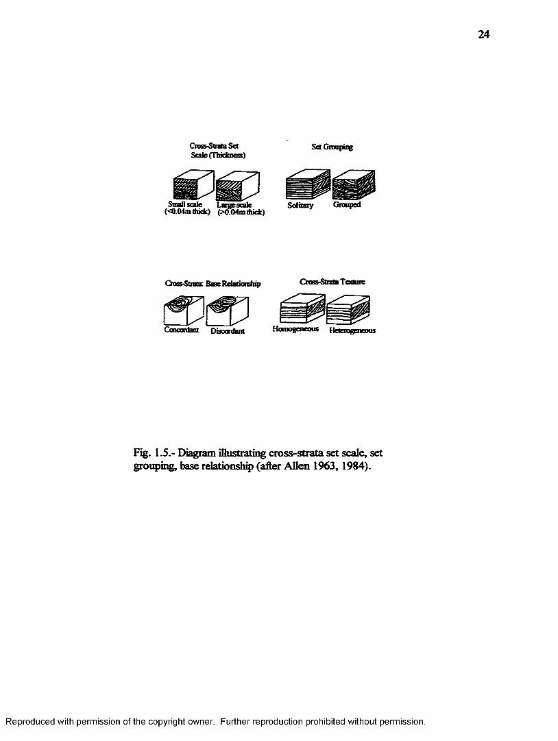
used is the degree of litho logical uniformity. Fig. 1.5 illustrates the descriptive terms

used in Allen's classification of Set scale, Set grouping, the Cross-strata base relationship

and Cross-strata texture. Fig. 1.6 illustrates Cross-strata shape and the shape of the

lower bounding surface. Using these six criteria, fifteen different types o f cross

stratification have been recognized (Table 1.6) (Allen 1963).

Campbell (1967) modified the McKee and Weir (1953) classification because he

believed that the former classification system was inadequate for quantitative

descriptions of stratigraphic organization Campbell sets up four component layers of a

sedimentary body. These layers are from smallest to largest, lamina, Iammasets, beds,

and bedsets.


24

Cross-Strata Set Scale (Thickness)

Set Grouping

Small scale Large scale (<0.04m thick) (X).04m thick)

Solitary Grouped

Cross-Strata; Base Relationship Cross-Strata Texture

Concordant Discordant Homogeneous Heterogeneous

Fig. 1.5.- Diagram illustrating cross-strata set scale, set grouping, base relationship (after Allen 1963, 1984).


25

Cross-Strata Shape

Rolling

Shape of Lower Bounding Surface

Sharp regular Sharp Irregular Planar/Tabular Curved

Cylindrical Scoop Trough Gradational

Fig. 1.6.- Classification of cross-strata shape and lower bounding surface shape (after Allen 1963, 1984).


26

The four layers are genetically similar, but differ in areal extent and the time interval

under which they were formed. In this classification system, lamina are the smallest

observable structure within the sedimentary body. A lamina set is a group of individual

lamina that are conformable and form a distinct structure within a bed. According to

Campbell, the bed reveals the principal layering, and is therefore the basic building block

of the sedimentary body. A bedset contains a number of superimposed genetically

related beds.The main difference between the McKee and Weir classification system and

that of Campbell’s, is that Campbell does not impose a limit on bed thickness unlike the

greater than one centimeter limit that McKee and Weir use. In Campbell’s classification

system, beds may be composed of lamina sets. This classification system differs from

other hierarchical systems that are less widely used in that it does not force adjacent beds

to be different lithologically, and the bed does not have to be composed of a

homogeneous Iithology. Table 1.7 shows a comparison between McKee and Weir’s

terminology and that of Campbell’s (Campbell 1967; McBride 1962; Bridge 1993).

Mesoscale Architecture (Facies and Facies Models)

Meso scale architecture refers to the study o f textures and sedimentary structures

on the scale of outcrops and well sections. This usually involves defining sedimentary

facies and constructing one dimensional vertical facies assemblages and facies models.

In 1669, Steno introduced the concept of facies, in which he defined facies as “the

characteristics of part of the Earth’s surface during a particular interval of time”

(Teichert 1958). Grossly (1838) introduced the modem usage o f the facies term by

defining it as the complete attributes of a stratigraphic unit including both

paleontological and litho logical characteristics.


27

Table 1.6.- Types o f cross-stratification, grouped by lower bounding surface shape, grouping scale and formation processes (after Allen 1984)

Set Scale Set Grouping Lower Bounding Surface Shape

Process Cross-StrataTypes

Large Scale Solitary Planar or irregular Due to migration of Alpha. Bela, solitary banks, sub- Gamma, Epsilonaerial or sob- and Xiaqueous, containing curving or linear fronts

Large Scale Solitary Cylindrical, sooop shaped orshaped

Bade filled hollows due to cutting and fiUing o f isolated channels, pits or hollows. Cutting and filling may not be simultaneous

Zeta, Eta, Them, and Iota

Small or Large Grouped Various Due to the migration of different sized ripple trams

A. Small Scale; Kappa, Lambda, Mu and Nu

B. Large Scale: Omikron and Pi

Table 1.7.- Comparison ofstratigraphic organization terminology o f the McKee andWeir system vs. Campbell’s terminology

__McKee and Weir (1953) Campbell (1967)____________

lamina or bed laminabfnin^ set

set (lamina or bed) bed

coset bedset

composite set

Walker (1984), suggests that the spatial relationships of rock volumes and their internal

characteristics must be compared to other modem well studied stratigraphic units in

order to properly identify facies. The reason for this is that it is generally assumed that a

facies designation will eventually be given an environmental interpretation.


28

Facies architecture is a term commonly used for mesoscale to large scale

architectural studies. Most facies architectural techniques involve the construction of

vertical facies assemblages and eventually facies models. A facies assemblage is defined

as the total attributes of a sedimentary body. This includes the geometry, areal extent,

continuity of the litho logic units, rock types, fossils and sedimentary structures of the

sedimentary body (Potter 1959; Miall 1990). A facies model is the depositional

environmental interpretation of the facies assemblage. Litho facies tend to organize into

depositional systems. A depositional system is defined as an assemblage of process

related facies (Fisher and McGowen 1967; Swift et al. 1991). The construction o f facies

assemblages and facies models relies heavily on the application of Walther’s Law.

Walther’s Law states that facies found in a vertical sequence were formed adjacent to

one another (Walker 1984; Miall 1990). This concept has great implications for

stratigraphers, because it implies that lateral facies relationships can be predicted by

investigating vertical facies successions. Walker (1984) states that any facies model

must fulfill three functions. First, the model must be the generalized case for a particular

depositional environment. Therefore, the model is to be used as a comparative tool for

local examples. The second function of a facies model is that it must set up a framework

to be used with future observations, and the third function is that it must act as a

predictor under newly encountered situations. Fig. 1.7 is an example of a classic facies

model, the Bouma sequence (Walker 1984).

Vertical Architectural Patterns. Vertical architectural patterns within sets and

co sets are thought to be the result of changing textural properties. Sets or cosets can be

homogeneous or heterogeneous with respect to textural properties and can create


29

recognizable patterns such as the above Bouma sequence. Visher (1965) described

systematic vertical variations of grain size within and between sedimentary structures of

fluvial origin in the Missourian of Oklahoma. Visher’s vertical depositional pattern

consists o f a basal unit containing trough cross bedding, followed by a laminated sand

zone. Above the laminated zone is a unit that is composed o f fine grained symmetrical

ripples. The top unit is a laminated clay and fine grained sand zone. This depositional

sequence has been recognized by Visher in both recent and ancient fluvial deposits. In

this vertical sequence, the mean and maximum grain size decreased upwards within

cosets as well as between cosets. The sorting also becomes poorer as you move up the

sequence. Visher interpreted this textural trend within the sequence as being the result

of an upward decrease in energy.

Allen (1984) reports that field observations have illustrated the vertical patterns

of grain size in cross laminated cosets. Fig. 1.8 shows Allen’s summary o f the

recognized patterns o f vertical grain size variations that have been reported. In this

summary, letters A, B, and S refer to specific types of climbing ripple or ripple drift cross

lamina sets. Type A ripple drift cross lamination consists o f climbing sets o f lee side

lamina. The stoss side is not preserved at all, and the preserved lee side lamina may be

either concave up or sigmoidal in shape. Type B ripple drift cross lamina is recognized

by climbing sets of lee side lamina and complete preservation of the stoss side lamina.

Stoss side lamina are relatively thick. Co sets of type B, usually do not contain graded

bedding. Type S, refers to sinusoidal ripples, and the stoss side is usually equal in

thickness to the lee side (Jopling et al. 1968; Allen 1973b). Parallel lamination is

represented by the P in Fig. 1.8 and D is the grain size diameter.


30

• > s • , • '* * . .1 • » ,. •

E(h)E ( t )

(D)C

B

Hemipefagic mud

Tarbidite mod

Interlaminations of silt and day

Rippled Bed

Upper Flat Bed

Sandy parallel laminations

Rapid deposition, Quick bed ?Massive or gradded bed*

Fig. 1.7.- The complete turbidite (after Walker 1984).


31

Stratification Sequence Gram Size ProfilesPattern t

Pattern 3

me*

te s t ”t a

Pattern 4r 7 r

E&33S

r

r

A

r 3-=~=_

aa 1

w* A

!?*»

iKara R^e

L

Fig. 1.8.- Vertical patterns of stratification and their related grain size patterns (after Allen 1984).


32

Pattern 1 has been recognized in the field by several researchers, (Sorby 1908;

McKee 1965; McKee et al. 1967; Coleman 1969) and shows a vertical sequence of

structures that grade from parallel lamina through type A and B cross lamina into S

typecross lamination. This type of vertical sequence of structures is usually found in

fluvial sediments, although some have been reported in glacial meltwater and turbidite

deposits. The grain size typically decreases vertically within and between cosets of this

sequence. Allen (1972b), reports that although it is rare to find a coarsening upward of

mean grain size in pattern I sequences, they exist in the Uppsala Esker. Allen (1984),

states that pattern 2 is a special geometrical condition in which the angle of climb is

uniform vertically. There is typically no vertical variation of grain size within and

between cosets in this pattern. R.G. Walker in 1963 reported a type C cross lamination

in which the angle of climb within cosets remained constant in muddy sand and silty

deposits. In this case, the mean grain size decreased upwards. Pattern 2 is usually

representative of turbidite, fluvial or deltaic facies. Jopling and Walker 1968 described

vertical grain size distributions in cosets illustrated by pattern 3. In this case, grain size

typically increases within and between cosets as you move upwards in the sequence.

Pattern 3 cycles are quite infrequent and are usually found only in glacial lake deltas

(Allen 1984). Pattern 4 illustrates repetitive cosets of various cross lamination types.

This pattern of cross lamina cosets usually consist of an upward fining o f the grain size,

and has been recognized from turbidite facies by Sorby (1908), and in the Uppsala Esker

by Allen (1972). In rare cases, an upward coarsening o f grain size has been recorded

(Allen 1984). All of these previous studies on vertical trends in grain size are good

preliminary attempts to understand the relationship between stratal architecture and grain


33

size variations, but much more work must be done in order to understand the full spatial

significance and relationship to grain size and permeability over several scales. Facies

models have been used by stratigraphers for quite some time, and they have been very

useful for the description of clastic environments but they are not adequate for

understanding large scale architecture (depositional sequences) or small scale

heterogeneities (Miall 1990; Bridge 1993). In order to folly understand the three

dimensional nature of sedimentary bodies, we need to break free o f one dimensional

vertical models.

Hierarchy o f Bounding Surfaces. In the previous section I explained that a

sedimentary body could be divided into a hierarchy of genetically related strata by

bedding contacts, and that McKee and Weir followed by Campbell were the first to

formalize classification systems. Brookfield (1977) showed that a four order bedform

hierarchy could be erected for aeolian deposits. The hierarchical bedform order of

Brookfield consists of impact ripples, aerodynamic ripples, dunes and draas.

This hierarchy of bedfbrms are separated by three internal bounding surfaces (Fig. 1.9).

First order surfaces are laterally extensive and are either convex up or flat lying bedding

planes that separate draas. Bounding sets of cross strata are second order surfaces.

Second order surfaces are analogous to McKee and Weir’s set designation. Third order

surfaces bind bundles o f lamina in cross strata sets and are designated as reactivation

surfaces. This surface is probably analogous to Campbell’s bminasets.

Allen (1983) made the first attempt to formalize a hierarchy of bounding surfaces

for fluvial deposits. He also recognized three major bounding surfaces, but reversed the

numbering order of Brookfield so that an opened ended numbering scheme was


34

Third Order

Cross-strata set bounding surfaces

Fig. 1.9.- Hierarchy of bounding surfaces (after Brookfield 1977).


35

developed. In Allen's classification of bounding surfaces, first order surfaces bound

individual sets of McKee and Weir. Second order surfaces are analogous to the coset

designation o f McKee and Weir, however they contain more than one lithofacies type.

Third order surfaces are laterally extensive. Miall (1988) expanded Allen's work to

incorporate the basin scale heterogeneity. In doing this, a six fold hierarchy was created

for fluvial sediments. The six fold hierarchy o f Miall is illustrated in Fig. 1.10. From this

classification system, Miall forwarded the idea of architectural elements, which has

gained wide spread use in recent years. An architectural element is defined as Iithosome

characterized by geometry, facies and scale. The implication of the architectural element

is that it represents the depositional product of sedimentary processes (Miall 1985,

1988). Fig. 1.11 illustrates the basic architectural elements defined by Miall in fluvial

deposits. In this classification system, first order surfaces are equivalent to Allen’s set

boundaries. The coset, as defined by McKee and Weir are bound by second order

surfaces in this system. Third order surfaces represent growth increments of macroforms

such as point bars or sand flats, and fourth order surfaces bound Miall’s architectural

elements. Fifth order surfaces are those that bound major sand sheets (channel fill

complexes), and six order surfaces bound channel groups or paleovalleys. The

architectural elements ofMiall clearly represents either facies or facies assemblages, and

this classification system has been extended to include large scale architecture.

Large Scale Architecture (Depositional Sequences)

Large scale architecture refers to the geometric relationships of sediment bodies

at the basin scale. The concepts o f sequence stratigraphy have been the most useful in

recent years in describing basin wide architecture.


36

W-K)*m

-IO, -IO* km

B .

flot

CH

bar

OALA

10-3000m-

Fig. 1.10.- Six fold hierarchy of bounding surfaces for fluvial deposits. A to E represents successive enlargements of fluvial unit showing the rank of bounding surfaces indicated by the circled numbers (after Miall 1985).


37

CH Channel

LA Lateral Accretion

SG Sediment Gravity Flow GB Gravel Bar and Bedform

SB Sand Bedform

DA Downstream AccretionLS Laminated Sand

OF Overbank Fines

Fig. 1.11.- Fluvial architectural elements (after Miall 1985).

Reproduced with permission of the copyright owner Further reproduction prohibited without permission.

38

Sequence stratigraphy is defined as the study o f the geometric relationship o f repetitive,

genetically related strata bounded by surfaces o f erosion or non-deposition, or their

correlative conformities, put within a chronostratigraphic framework (Van Wagoner et

aL 1988). The basic unit o f sequence stratigraphy is the depositional sequence. A

sequence is recognized as genetically related strata that are bounded by unconformities

and their correlative conformities. Each sequence can be sub-divided in smaller units

known as system tracts (Mitchum 1977). System tracts are recognized by their position

and stacking patterns within the sequence and are composed o f parasequences.

Parasequences are defined as a succession o f conformable genetically related strata that

are bounded by marine flooding surfaces and their correlative surfaces (Van Wagoner

1985; Van Wagoner et aL 1988; Allen and Allen 1990). Marine flooding surfaces are

surfaces that represent abrupt changes in water depth and are used to separate older

strata from younger strata (Van Wagoner et aL 1988). Parasequences may be grouped

into parasequence sets, which are defined as genetically related parasequences.

Parasequence sets have been recognized as forming distinctive stacking patterns that are

often bounded by marine flooding surfaces (Van Wagoner 1985). Correlating and

mapping of sedimentary rocks using this nomenclature, is accomplished by defining the

boundaries between sequences, parasequences, and parasequence sets. It is believed that

rates of subsidence, eustacy and sediment supply all contribute to the formation of

sequences and their stratal components (Fig. 1.12), (Van Wagoner et aL 1988).

In 1977, Peter Vail and colleagues from Exxon constructed a chart of relative sea

level versus time. This chart is known in the literature as the Vail curve, and was

constructed by using seismic reflection techniques. The limits o f onlap and toplap within


39

coastal facies of marine sequences as recorded by seismic refection methods are thought

to be the best indicators o f relative sea level fluctuations. Coastal onlap is considered to

be indicative of a relative rise in sea level, whereas coastal toplap is indicative of a

standstill of relative sea level. A relative fell in sea level is represented by a downward

shift in coastal onlap. Fig. 1.13 illustrates the geometric relationships of onlap and

toplap in relation to relative sea level fall, rise or standstill (Vail et al 1977; Allen and

Allen 1990).

Stratal architectural models utilizing sequence stratigraphic concepts have been

used extensively in order to predict reservoir facies in deep water environments. Self

and colleagues (1993) investigated the usefulness of sequence stratigraphic models in

predicting reservoir facies of the Plio-Pleistocene in the Gulf o f Mexico. They concluded

that current sequence stratigraphic models are too simplistic, and fail to incorporate

complex forcing mechanisms other than eustatic sea level fluctuations. Therefore, Self

argues that the predicted lithology is often inaccurate when compared to the actual

lithology recovered in wells. The authors suggest using an empirical approach which

incorporates the correlation of oxygen isotope data and fbraminiferal analysis to

sequence boundaries. This study demonstrates the need for a different approach to

successfully predict lithology. This approach may work for large scale basin wide

architecture, but would not work for the small scale heterogeneity that is often

encountered in aquifers.

Architectural Classification used in this Study

Facies modeling has been the method of choice for most stratigraphic

organization studies and has had some success at describing sedimentary environments.


40

V / / / A

7 / / / A

btised Valey

Fig. 1.12. - Features of a sequence and it's associated system tracts, boundaries within systems traces are parasequences. HST is high stand systems tract, LST is low stand system tract, TST is transgressrve systems tract, SB1 is type 1 sequence boundary and mfs is maximum flooding surface (after Vail 1987).


41

(a) RELATIVE RISE

Terrigenous influxCoastal

(c) GHAOOAL RELATIVE FALL Terrigenous influx

Erosional truncation

" v w w a p RelafiveR n all la*of sea level

encroachment Iniial depositional surface

Chronostrahgraplucsurfaces

(b) R&AT1VE ST1LLSTAND

Terrigenous Mux — ToplapRelative stflbtand

Scale

Tens to thousands of km

(d) RAPID RELATIVE FALL Terrigenous M ux Underlying unconformity

Surface associated wMi basinvrard shat

If-Y-j Non-marine coastal deposts | | Littoral deposts

KH1 Marine deposits

Fig. 1.13 - Stratigraphic consequences o f eustatic sea level changes (after Vail et al. 1979).


42

However, one dimensional vertical models are inadequate for the understanding of

sedimentary heterogeneity. In an important study conducted by Liu et al. 1996, several

permeability and porosity measurements were made on the Triassic Hawkesbury

Sandstone in Sydney, Australia. Sedimentological and geo statistical approaches were

utilized in order to characterize the horizontal and vertical permeability and porosity

variations in braided river depositional systems. The results o f this study revealed that

there was a high degree o f variability within the permeability data, and that this

variability is not consistent with fractal models based on a Gaussian Normal probability

distribution. The authors also discovered that when they sub-divided the sandstone into

genetically related sedimentary facies, the predictability o f the permeability distribution

was significantly improved. Although Liu has successfully shown that facies analysis

greatly increases the ability to predict hydraulic properties, even leading edge facies

analysis could stand a significant improvement. Sequence stratigraphic methods have

also been used extensively, but this approach is only reasonable on the basin scale, for it

also neglects small scale heterogeneity which may be important to secondary textural

properties.

Architectural elements and numbering o f bounding surfaces are the latest

approaches to understanding stratigraphic organization. Numerous studies have been

published attempting to relate secondary textural properties to these elements or

bounding surfaces. Davis et al. (1997) attempted to relate fluvial bounding surfaces and

the permeability correlation structure in outcrops o f the Sierra Ladrones Formation,

Albuquerque Basin, New Mexico. The authors concluded that the results suggest that

fluvial bounding surfaces provide a geological basis for modeling heterogeneity in


43

alluvial deposits. Both of these studies are an excellent start in the understanding of

permeability correlation structure and how it relates to geologic structures; however

neither of these studies incorporated ideas from Bridge’s (1993) review paper. In his

review paper, Bridge (1993) critiques several current methods used to describe and

classify sedimentary deposits o f fluvial origin. Bridge argues that the practice of

numerically ordering bounding surfaces rather than the strata themselves is often difficult

to apply uniformly. He also points out that architectural elements or lithofacies codings

are not mutually exclusive, and tend to either be misleading or incorrect. Bridge also

states that the use of one dimensional vertical sequences o f litho facies is obsolete, and

stresses that a simple classification based on easily measured parameters should be used.

I agree with Bridge’s comments on these methods, and therefore suggest that the simple

classification of McKee and Weir (1953) be used and extended to the larger stratigraphic

scales. In the stratal architecture classification system that I am proposing to use,

individual strata (lamina or beds) organize to form sets o f strata, and these sets of strata

organize to form cosets of strata. The coset is the largest category in the McKee and

Weir classification system and can vary significantly in sedimentary structures and

lithology. Therefore, the term coset overlaps and is analogous to the smallest facies

category, that of facies volume. On larger stratigraphic scales, facies may organize into

depositional systems. Depositional systems may consist o f fining upward or coarsening

upward facies successions, that rest on or are capped by a source diastem (Swift et a l

1991). Therefore, the depositional system overlaps with the concept o f a parasequence

as defined by sequence stratigraphic nomenclature. Depositional systems may further

organize into a set of depositional systems, which is analogous to a sequence, the


44

fundamental unit of sequence stratigraphy. It is important to keep in mind that facies and

depositional systems are usually autocyclic in nature, while conventional sequence

stratigraphic concepts are generally thought to be allocyclic in nature. Table 1.8

illustrates the relationship between successive stratigraphic organization terms.

Table 1.8.- Scales o f stratigraphic organization used in this study

Stratal (small scale) Facies (mesoscale) Sequence (large scale)

cross-stratum

cross-strata set

cross-strata coset fades

depositional system parasequence

depositional sequence

THE STUDY AREA

General Geology of the Eastern Shore

The Deknarva Peninsula is part of the Middle Atlantic coastal plain bordered on

the west by the Chesapeake Bay and on the east by the Delaware Bay and Atlantic

Ocean (Fig. 1.14). The Oyster site is situated on the Iagoonal side o f Virginia’s Eastern

Shore landward of the outer barrier island chain. In this area, the coastal plain deposits

consist of unconsolidated sediments of Cenozoic age ranging from 65 million years old

to the present. The Upper Pleistocene deposits are composed of gravel, sand and clay

formed in marginal marine and estuarine environments during high stands of sea level

(Mixon 1985; Schiedler et aL 1984). The Quaternary was dominated by periods of

cyclic growth and retreat of the polar ice caps, with a period of approximately 100,000


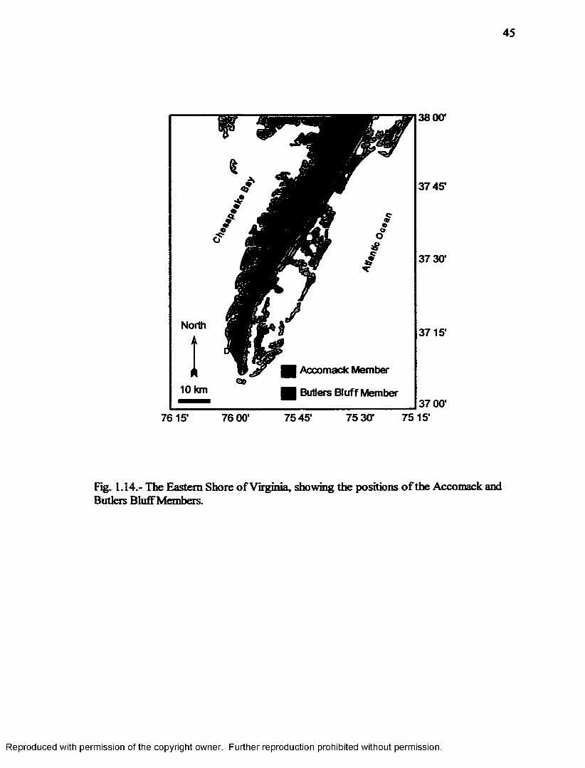
45

North

10 km

38 00'

Accomack Member

Butlers Bluff Member

3745’

37 30*

3715*

37 00’7615’ 76 00’ 7545' 75 30' 7515*

Fig. 1.14.- The Eastern Shore of Virginia, showing the positions o f the Accomack and Butlers Bluff Members.


46

years. Each ice advance caused sea level to drop about 125 m, and the architecture of the

Upper Pleistocene deposits exhibits this pattern. Periods of low stand followed by inter

glacial high stands of sea level resulted in the formation of a coastwise stepped

topography known as terraces. These terraces, which step down towards both the

Atlantic Ocean and the Chesapeake Bay, are separated by low tying linear scarps. The

scarps (Mappsburg and Cheriton), have been interpreted to be ancient shorelines of

marine and estuarine origin (Colquhoun et aL 1991; Mixon 1985). The Chesapeake Bay,

the largest estuary in North America, was formed by the drowning of the lower

Susquehanna River during the post glacial sea level rise, amplified by lithospheric

subsidence. The modem day configuration o f the Bay developed over the past two sea

level cycles (Mixon 1985). At approximately 240,000 yrs. BP., the Accomack Spit,

precursor o f the Eastern Shore Peninsula, built seaward across the mouth of an ancestral

Chesapeake Bay during a time when sea level was twenty meters higher than at present.

During the 240,000 year high stand, a barrier spit formed as an extension of the barrier

system of the Delmarva coast, in response to the southwest transport of sand in the zone

of shoaling and breaking waves. Through stratigraphic analysis of the Delmarva

Peninsula, Mixon (1985) has designated this deposit as the Accomack Member o f the

Omar Formation.

During the subsequent sea level fall, the shoreline retreated back across the shelf

and down onto the upper slope, stranding the Accomack Spit in the re-exposed

Susquehanna Valley (Mixon 1985). When sea level rose again, a second barrier spit was

emplaced, further restricting the mouth of the Chesapeake Bay. This deposit has been

named the Nassawadox Formation (Mixon 1985). Mixon (1985) suggests that this


47

deposit accumulated approximately 120,000 years BP. The oceanic side of the

Nassawadox Formation is made up of mostly well sorted, medium to coarse grained sand

that has been deposited in surf zone and tidal bay mouth environments. This sub unit is

known as the Butlers Bluff Member, and was named after exposures at Butlers Bluff,

Kiptopeake State Park (Mixon 1985). The Oyster site lies completely within the Butlers

Bluff Member. The Bay side of the Nassawadox Formation consists o f finer grained

sand, richer in clay, which was deposited in a back barrier environment. These deposits

have been designated as the Occohannock Member. The Stumptown Member is the

third Member o f the Nassawadox Formation, and was deposited in the Eastville

paleovalley, incised into older deposits during the earlier sea level fall (Mixon 1985),

(Fig. 1.15).

The Nassawadox spit pro graded across the ancestral Chesapeake Bay as a result

of sand being bypassed along the oceanic side o f the spit driven by the longshore current.

As the sand approached the edge o f the spit, some o f it was transported by tidal currents

and was deposited onto the tidal sand shoal of the bay mouth. Most of the sand was

driven around the tip of the spit by wave refraction. As the fluid power decreased in this

area, sand was deposited in incremental steps around the tip o f the spit. As time

progressed, the edge of the spit prograded across the bay mouth, overrunning the tidal

shoaL As a result, time surfaces on the oceanic side of the spit dip seaward, and curve

towards the west dipping southward. The Nassawadox spit is underlain by the tidal

shoal deposit (Fig. 1.16), (Parsons and Swift 1995; Mixon 1985). After the deposition

of the Nassawadox Formation, sea level fell again, until approximately 18,000 years BP.,

when sea began to rise again. Sea level rose quickly (0.1 my'1), to about 7,000 years BP.


48

Helen20-

10-aea level -

10-*

20-

3o-

4o-

5o-60-

Nassawadox Formation: Butlers Bluff and Occohannock Members, moderately sorted to well sorted, fine to coarse sand.

Stumptown Member Unit C, muddy and shelly fine sand; Unit B, clay-silt; Unit A, gravelly sand and sandy gravel.

Fig. 1.15.- Cross section showing the stratigraphic relationship of the members of the Nassawadox Formation (after Mixon 1985).

OKrifaMScarp Mapps bar? scarp


49

Since about 4,000 years BP. sea level has men at a much slower rate. Presently, the sea

has risen to the level at which it was during the deposition o f the Nassawadox

Formation. A Holocene barrier lagoon system has moved in across the shelf as sea level

rose, and is currently backed up against the Mappsburg Scarp, the shoreline of the

Nassawadox high stand (Mixon 1985; Parsons and Swift 1995).

The Oyster Site as a Natural Lab

Oyster, Virginia has been selected by the Department of Energy to be the site

where experiments in bacterial transport in heterogeneous porous media wDl be

conducted. The Oyster Borrow Pit is an excellent location to study the heterogenic

nature of shallow marine aquifers because o f its accessibility, clean sands and truly

heterogenic nature. The goal of this study is to relate scales of stratigraphic organization

to the distribution of grain size, permeability and facies in shallow marine deposits. As

pointed out earlier, one o f the most significant problems in stratigraphy and

sedimentology is that classical facies models and the use of borehole logs are inadequate

in constructing the detailed anisotropy that exists in sedimentary deposits. Another

problem that needs to be resolved is that very few studies have related reservoir

characteristics to the depositional environment. The Oyster site is a suitable place to

investigate these problems. The classical use of facies models and even sequence

stratigraphic concepts require a considerable amount o f inference and can not resolve

many uncertainties in the stratigraphic architecture. However, exposures at the Oyster

site will allow us to resolve the relationship between scales o f stratigraphic architecture

and its role in controlling the spatial distribution of important reservoir and aquifer

characteristics such as grain size and permeability.


50

( a ) t r a n s p o r t p a t t e r nPR O G R A D IN GR E C U R V E D SAND SPIT ______

PARABOLIC TIDAL SHOAL

© S U C C E S S IV E P O S IT IO N S O F O U T E R S P IT S H O R E L IN E

ZONE O F RAPID C O A STW ISE ADVANCE ZO N E OF SLOW

OSCILLATORY SEAW ARD ADVANCE

© IN T E R N A L G E O M E T R Y O F S P I T

SU R FA C E S OF EQUAL TIME ARE CU RV ED WITHIN SPIT

Fig. 1.16.- Evolution of the Nassawadox Spit.


51

Facies Erected in the Study Area

The samples used in this program were collected during the field campaigns of

the subsurface science program (Department of Energy) in 1994 and 1996. In 1994, the

Oyster borrow pit was exposed for the first time, and five measured sections were

constructed. Grain size and permeability samples were collected in a preliminary

investigation. In 1996, researchers returned to the Oyster pit in order to fully

characterize the site. Three tiers were exposed that were twenty meters in length and

two meters in height. Grain size and permeability samples were also collected, and the

stratal geometry was mapped. All of the beds in the Butlers Bluff member were

deposited in a Shoreface setting (1-15 m water depth) and constitutes a shoreface facies.

Mixon (1985) describes the Butlers Bluff Member as an 18 meter thick fine clean sand to

coarse sand and gravel unit. This unit consists of cross-bedded deposits and it overlies

the Stumptown Member. The most common feature o f this unit are the large scale

trough cross beds and the ghost casts of Spisula solidissim a as well as other bivalves.

Mixon (1985) recognizes two distinct sediment types or facies within the Butlers Buff

Member. The first type consists of poorly sorted, medium to coarse pebbly sands

composed mostly of quartz. This sediment type occurs mostly in the upper Butlers Bluff

Member. In the Lower Butlers BlufE, the d o minant sediment type or facies consists of

well sorted, medium to fine sands with abundant black heavy minerals. During the first

field campaign in 1994, three distinct sediment types or facies were recognized in the

Oyster pit, based on the examination of feces excavated, photomosaics and on laboratory

grain size analysis o f samples collected. The fecies recognized are, a Cross-Stratified

Sand Facies, a Horizontally Stratified Sand Facies and a Shelly Gravelly Sand Facies.


52

HYPOTHESIS TO BE TESTED

I propose to investigate the sedimento logical sources of variation of grain size,

and permeability in shallow marine deposits by relating the small scale stratigraphic

organization of the Oyster deposits to these properties. I propose to test the hypothesis

that models of stratal architecture are more efficient predictors of grain size and

permeability than are facies models in shallow marine sands. An important issue to be

resolved by this study is the extent to which the permeability and grain size correlate

with the distribution of set boundaries.

THESIS LAYOUT

Chapter I of this dissertation serves as an introduction to the study, and ends with

the hypothesis to be tested. Chapter II describes the methods that will be used to

address the hypothesis. Chapters HI and IV are the results section o f the dissertation.

Chapter III focuses on the stratal architecture of the Oyster Pit, and Chapter IV is the

results of the geo statistical analysis. Chapter V is the discussion and conclusions.


53

CHAPTER II

METHODS OF STUDY

INTRODUCTION

Approach

The purpose of this study is to understand scales of physical heterogeneity that

relate to grain size and permeability distributions within shallow marine deposits. In the

undertaking of such a study, several important questions arise that help us to understand

how scales of stratigraphic organization affect the distribution o f grain size and

permeability, as well as the development o f a better understanding of how primary

textural properties affect secondary properties. These important questions that must be

addressed are:

(1) What are the predominant grain size and permeability correlation length scales?

(2) What is the vertical distribution of grain size and permeability within and between

sets?

(3) What is the relationship between grain size and permeability?

(4) What is the relationship between grain size and set thickness?

(5) Is there more variability in the grain size and permeability distributions within sets or

between sets?

(6) Is there more variability in the grain size and permeability distributions within or

between strata cosets?

In order to answer these questions, I propose to use a combination of field, laboratory

and geo statistical techniques. The remainder of this chapter is devoted to the

explanation of these techniques and how they will help to construct the physical


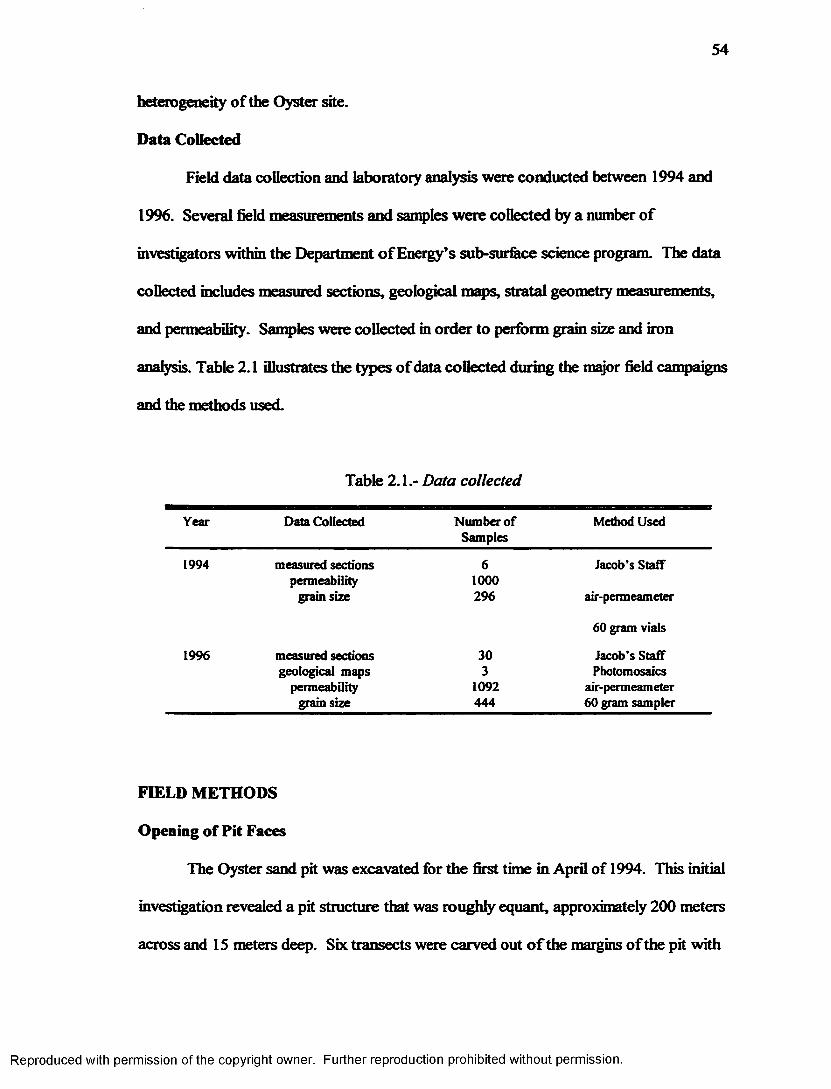
54

heterogeneity of the Oyster site.

Data Collected

Field data collection and laboratory analysis were conducted between 1994 and

1996. Several field measurements and samples were collected by a number of

investigators within the Department o f Energy’s sub-surface science program. The data

collected includes measured sections, geological maps, stratal geometry measurements,

and permeability. Samples were collected in order to perform grain size and iron

analysis. Table 2.1 illustrates the types of data collected during the major field campaigns

and the methods used.

Table 2.1.- Data collected

Year Data Collected Number of Samples

Method Used

1994 measured sections 6 Jacob’s Staffpermeability 1000

grain size 296 air-permeameter

60 gram vials

1996 measured sections 30 Jacob’s Staffgeological maps 3 Photomosaics

permeability 1092 air-permeametergrain size 444 60 gram sampler

FIELD METHODS

Opening of Pit Faces

The Oyster sand pit was excavated for the first time in April of 1994. This initial

investigation revealed a pit structure that was roughly equant, approximately 200 meters

across and 15 meters deep. Six transects were carved out o f the margins of the pit with


55

the aid o f a shovel, and a pace and compass map of the area was constructed. In April of

1996, the Oyster pit was reopened for an intensive sampling and interpretation of the

reservoir properties and stratal architecture o f this area. The initial 1994 study was not

designed to determine the horizontal correlation structure or to take unbiased statistical

measures of the aquifer properties. The pit was excavated with the aid o f a backhoe, and

three 20 meter long and 2 meter high outcrops or tiers were constructed. The tier feces

were then smoothed with a shoveL

Measured Sections

Detailed measured sections were made for each transect using a Jacob’s staff.

The Jacob’s staff is a pole that is one and a half meters in height and contains a

clinometer and sighting bar. The Jacob’s staff is used to measure stratigraphic

thicknesses accurately and quickly (Lewis 1984; Miall 1990). Visual estimates of grain

size were taken with the aid of a hand lens and a grain size comparator card.

Paleocurrent measurements were also taken. In 1996, stratigraphic sections were

constructed for each tier every 2 meters. Primary structures and facies type were

identified in each. Visual estimates of grain size were made, and paleocurrent

measurements were also taken.

Geological Mapping

Detailed geological maps of each o f the tiers were constructed. Horizontal

distance of each tier was measured with a tape measure and painted on the face itself in

one meter increments. Nails were put into the tops and bases of each face at every meter

and were then surveyed in order to create an accurate map in northings, eastings and

elevation. Stratal set boundaries were also mapped on the geologic base map in order to


56

correlate the geometry of the deposits to the samples collected. Digital photographs of

the outcrop and sampling locations were taken by professional photographers. Each

photograph contains a scale and color chart. All photos were placed on CD, and used

to construct photomosaics of the outcrop.

After all of the nails and samples were surveyed, a grid containing the nail

locations and samples for each tier were created using ROCKBASE™, (Rockware

1991). The geological maps and the ROCKBASE™ maps were then scanned into

Adobe Photoshop®. The ROCKBASE™ map was scaled to the geological maps and

then put as a separate layer over the geological map for each tier. This gives an accurate

placement for all samples taken.

Sampling Procedures

Sampling was conducted by using a staggered grid. The sample grids were two

meters long and one meter high. Individual grid cells were 10 cm by 10 cm.

Measurements of aquifer properties were made over several scales in order to construct

the physical heterogeneity of the location, and to determine the scale controlling these

properties. Each sample was then surveyed. Bias samples were also taken to insure that

samples would cut across set boundaries. Samples were labeled such that they could be

correlated to one another. This was done by using a unique eight digit sample number.

The first two digits represent the year in which the sample was collected. The third and

fourth digits represent the grid frame locations. The fifth, sixth and seventh numbers

represent the grid box number. The last digit represents the sector o f the grid the sample

was taken from. Each grid is divided into quarters, and the sectors are labeled in a

clockwise manner (Fig. 2.1), (Mcling and Higgs 1996).


57

10 cm

10 cm Y \' 2

3 *4

1 m

2 m

Fig. 2 . 1 Sample grid used to place samples on the outcrop face.


58

Grain Size. Grain size samples were collected from the grids for detailed

laboratory analysis. A 60 gram sampler was used to collect the sample, and each sample

was labeled with a unique Sediment Dynamics Lab number (SDL#), for quality control

purposes. A total o f596 grain size samples were collected from the pit over the two

sam pling cam paigns.

Permeability. Field measurements of permeability in the Oyster pit were

conducted by the use of a portable air-minipermeameter. The air-minipermeameter is an

economical way to obtain several hundred measurements of hydraulic conductivity in a

short period of time. This allows the investigator to determine the spatial distribution of

permeability in an outcrop or petroleum reservoir. This instrument works by measuring

the rate at which a glass syringe piston displaces a known volume of air, which is

injected through a tip seaL The permeability is calculated from the relation described

below by Goggin et al. 1988. In equation 2-1, K is the hydraulic

w ,aG„(bD)(P]-Pl) <2' °

conductivity [m/s]; p. is the air viscosity [Pa.s]; q is equal to the volumetric flow rate

[m3/s]; PI is the pressure at tip seal [Pa]; Po is equal to the atmospheric pressure [Pa]; a

represents the inner radius o f tip seal [m]; b represents the outer tip seal radius [m]; bD is

the dimensionless tip seal radius, and is equal to [b/a]; and Go(bD) is a dimensionless

geometric factor (Davis et aL 1994). Permeability is determined from the Darcy

equation.

Stratal Geometry Measurements. Detailed measurements o f the thickness and


59

width o f individual strata, strata sets and cosets were made for each tier. Average values

o f these properties and the standard deviations were calculated for every set in each

coset. Individual cosets are determined through the analysis of set thickness, lamina

geometry and grain size characteristics. The stratal geometry statistics enables the

construction of normative sets, as well as the relationship between mean grain size and

set thickness.

LABORATORY METHODS

Grain Size Analysis

Each sample was first labeled with a unique sediment Dynamics Laboratory

Number for quality control purposes. Samples analyzed for grain size were first dried,

then split down to approximately a 30 gram sample. Sediments in the range o f -2 to

2.75 phi were analyzed using standard methods of sieve analysis in quarter phi units

(Folk 1974). Sediments that were finer than 2.75 phi were analyzed using an

Electrozone particle size analyzer. The particle analyzer measures the volume of the

particles as they enter a particular size orifice tube. The sediments are suspended in an

electrolyte and are drawn into the orifice tube where an electrical impedance is created

across an electrode. The impedance is directly proportional to the volume o f the

particle. The signal is magnified and the volume is recorded. This is a more accurate

way of measuring fine sands and muds than pipette analysis because it is not sensitive to

shape or density effects (Milligan and Kranek 1991).

Geostatistical Analysis

Textural Properties. The first step in understanding the relationship between

scales of stratigraphic organization and textural properties is to calculate basic moment


6 0

parameter statistics of the samples collected in order to determine if distinct patterns can

be seen. Mean grain size, sorting (standard deviation), skewness, kurtosis and percent

gravel were determined for all grain size samples. Standard box plots were also

constructed for the permeability data. Bivariate plots of textural properties were

constructed to investigate relationships between sedimentotogical parameters and to

help construct the depositional environment

Normalization o f Textural Properties to S et Geometry. As was pointed out

earlier, measurements o f individual strata, and strata sets within each coset are used to

define a normative set. In defining the set geometry, the Y axis represents the set

thickness, X is the set width and Z is the set length. Individual lamina may act as grain

size contours indicating a fining upward sequence within a set. In order to understand

the vertical distribution of grain size and permeability within strata sets, sample locations

were assigned new coordinates based on their position relative to their height from the

base of the strata set. In this coordinate system, the y axis is the now the vertical

distance from the base of the set to the top of the set, and samples were assigned values

between 0 and 1, (Fig. 2.2).

Variogram Construction. The basic tool for the analysis of spatial structure is

the semivariogram. Semivariogram analysis has been utilized by mining geologists for a

number of years to characterize the correlation length scales o f the particular property o f

interest. The semivariogram, also called the variogram, is a measurement o f the mean-

squared differences between individual sample values at user defined separation

distances. The variogram is calculated with the following formula:


61

Y(/7>=2 ^ ) E[Z(X' +/,)"Z(X/)]2 ( 2 " 2 )

In equation 2-2, y (A) is known as the variogram statistic, z (x,) is the observation at

position (xy), /z is the distance between observations and n(h) is the number of data pairs

separated by h (Hess et aL 1992; Davis 1973; Pannatier 1996). When the distance

between observations is zero, every data point is being compared to itself therefore the

semivariance is zero. When the distance between observations is small, the data points

are usually very similar in magnitude and the semivariance is smalL As the distance

between observation becomes larger, the observations are not as closely related to each

other. In this case the semivariance increases. At some distance, the observations are

no longer related to each other at all, the semivariance no longer increases and the

semivariogram develops a flat region known as the silL This occurs because as the

distance between the observations increases the squared differences will eventually equal

the variance around the average value under stationary conditions. The distance where

the semivariance approaches the variance is called the range o f the variable. The range

defines the distance over which observations are related to one another (Fig. 2-3),

(Davis 1973). Semivariogram analysis was performed with the aid of the commercial

program VARIOWIN0, which is a collection of programs designed for the analysis of

spatial data.

Analysis o f Variance (ANOVA). One of the most universally used statistical

techniques for analyzing data is analysis of variance. This technique has been used

extensively in the biological and social sciences, and has found increasing applicability to


62

Y - SetTUekneaa

X = Set Width

2 . Set Length

dffdr * Mean Set Dimensions

0

y “ Vertical Distance from set trough (0-1)

X “ Hastngs (meters)

Fig. 2.2 Definition sketch for a normative set, and the normalization o f samples to set geometry.


63

Sillfebo•ca t

Range

Separation Distance

Fig. 2.3.- Definition sketch of a typical variogram.


64

This technique has been used extensively in the biological and social sciences, and has

found increasing applicability to paleontological and sedimentological studies. The

variance is defined as the variability o f a particular group of data. In an analysis of

variance, data are collected and organized such that the variability among the grouped

data is compared to the variability between the groups. The variance is calculated as the

sum of squared deviations of the observations from the group mean divided by the

degrees o f freedom. In equation 2-3, s2 is the variance, x is an individual observation,

(2 .3)A M ' ’

AT is the group arithmetic mean and N is the number of observations. The total variation

is derived by calculating the average squared deviations of the observations from the

grand mean (Dowdy and Wearden 1991; Krumbein and Miller 1953).

E £ O' -yf*-*•! 'S'J (2-4)rta- 1

In equation 2-4, n represents the number of observations and a is the number of groups.

Total variance is broken into two parts, the within-group variance and the among-group

variance. The within-group variance is the average squared deviations of the


65

observations from the group average (Eq 2-5). This is also known as the pooled

variance. The among-group variance is calculated by taking the average

E, E %-yf 2a fn -l)

squared deviations of the group averages from the grand average. This value is then

multiplied by the number of observations in each group (Eq 2-6). This type of analysis of

variance is known as a one-way completely randomized ANOVA.

Y i. (y -y)2”[— V ] (2-6)a -l

The ANOVA tests the hypothesis that the means between groups are equal This is

known as the null hypothesis, and the alternative hypothesis is that at least one of the

means of the groups is not equaL The null hypothesis is tested by calculating an F ratio.

The F ratio is defined as the ratio of the among-group variance to the within-group

variance. This value is then compared to the critical F value for the particular degrees of

freedom in the test and the desired a (confidence level). If the critical value is exceeded

by the F ratio, then the null hypothesis is rejected, and one must conclude that at least

one inequality between the group means exists. The analysis o f variance in this case will


66

be used to determine if significant variation exists within or between individual strata

sets and cosets. There are three basic assumptions made when undergoing such an

analysis. The three requirements for this test are the assumption of additivity, normality

o f data groups and the homogeneity o f variance. The assumption of additivity requires

that there is no significant interaction between individual observations. These three

conditions will be explained and examined in detail in Chapter IV. Due to the large

number of observations, the analysis o f variance tests were conducted with the aid of the

statistical software package known as IMP®.


67

CHAPTER EQ

ARCHITECTURE OF THE OYSTER SITE

INTRODUCTION

Sediment o logical investigation o f the Oyster Pit sediments during the 1994 and

1996 field campaigns revealed very coarse, poorly sorted to fine grained well sorted

sediments. Lenticular pebbly lag deposits occur in the upper two-thirds of the section

exposed. Fig. 3.1 illustrates the dominant sedimentary feature o f cross-stratification

which occur in cross-strata sets. Each cross-strata set is composed of trough shaped

lamina. Pelecypod casts replaced by hydrous iron oxide, as well as vertical burrows of

Spisula solidissima occur throughout the upper Butlers Bluff Member. Hydrous iron

oxide staining of the sedimentary deposits tend to outline individual cross strata sets.

During the 1996 field campaign the pebbly lag deposits were found to occur generally at

the base of cross strata sets. The lower third of the Butlers Bluff Member consists of

parallel lamina that are nearly horizontal, and tend to have less iron oxide staining (Fig.

3.2).

FACIES ARCHITECTURE

During the initial examination o f the Oyster Site in 1994, three facies were

recognized based on sedimentary structures and grain size gradients. The three facies

identified are a Cross-stratified sand facies, a Shelly gravelly sand facies and a

Horizontally stratified sand facies. The Spring 1996 field campaign opened three tiers

measuring twenty meters across by 2 meters high. This gave the researcher a full view of

the facies relationships in the Butlers Bluff Member. Close inspection of Fig. 3.1 clearly

demonstrates that the Shelly-gravelly sediments are generally located a the base of


68

Fig. 3.1.- Photograph of trough cross-stratification at the Oyster Site. Note the basal gravel lags in cross strata sets (arrows).

Fig. 3.2.- Photograph illustrating sediments from the lower Butlers Bluff Member.


69

Cross-stratified sets. Therefore, the Shelly Gravelly sand facies and the Cross-stratified

sand facies are more closely related to each other then they are to the Horizontally

stratified sand facies and may be considered subfacies of a common cross stratified

facies. A new facies was also recognized during the 1996 investigation. Sediments

exposed near the base of Tier 3 (bottom of the section) contained coarse gravelly

sediments with wavy bedding. This facies which I will call Micro cross stratified sand

facies occurs beneath the Horizontally stratified sand facies. Unfortunately, due to pit

instability, only a small portion of this facies was exposed (Fig. 3.2).

The distribution of facies within the Oyster Site can best be revealed by the

construction o f measured sections. Measured sections were constructed at every two

meters horizontally for the entire Oyster Site. Fig. 3.3 through 3.6 illustrates the lateral

and vertical facies distributions. From these measured sections it is clear that the upper

two-thirds of the Oyster Site is dominated by the continuous Cross-stratified sand facies

with lenticular pebbly deposits that make up the less continuous Shelly gravelly sand

facies. The average grain size of the Cross-stratified sand facies is 1.60 phi and the

average sorting is 0.74. The average gravel content is 1.72%, and the samples were all

very negatively skewed. The Lower third o f the Oyster Site consists mostly of the

Horizontal stratified sand facies. The average grain size of the Horizontally stratified

sand facies is 2.57 phi, and contains the best sorted deposits. The Micro cross stratified

and the Shelly gravelly sand facies have similar textural characteristics to those of the

Cross-stratified sand facies (Table 3.1). The Cross-stratified sand facies makes up more

than two-thirds of the entire Butlers Bluff Member, and the Horizontally stratified sand

facies makes up 15 percent.


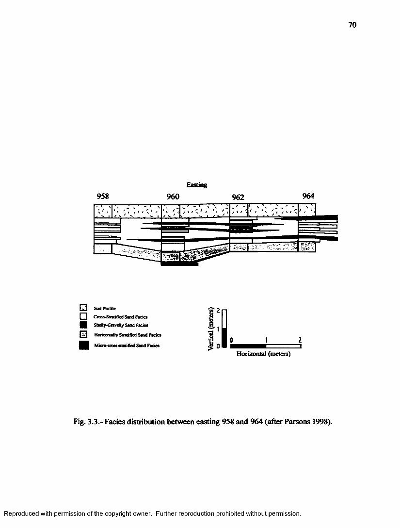
70

Easting

958 960 962 964

Sod ProfileCross-Stratified Sand Facies Shelly-Gravelly Sand Fades

Horizontally Stratified Sand Fa

Micro-cross stratified Sand Fades

I 2•3? °

1Horizontal (meters)

Fig. 3.3.- Facies distribution between easting 958 and 964 (after Parsons 1998).


71

Easting

964 966 968 970

Horizontal (meters)

□ Sod Profile□ Cross-Stratified Sand Facies I } Shefiy-CnveOy Saad Facia

□ Horizontally Stratified Sand Facies

I I Micro-cross stratified Sand Facies



72

Easting

□ Sod Profile

□ Cias-Stmificd Sand Facies

~ 2 n H Shetty-CnveOy Sand Facacs

^ 11 I - I Horizontally Stratified Sand Facies

i^ — - - Zi IH Micro-cross stratified Sand FaciesHonamol (meters)



73

Easting976

978

' /

/

\

/ ,.

- - 1 I V 7' ' N - - \ ^ ' ' v ---------- \ < 1

1 _____ r1

980 982

- i l - v . —

□ Soil Profile

□ Cross-Stratified Sand Facies

■ Shelly-Gravelly Sand Facies1*2

H s Horizontally Stratified Sand Facies

■ Micro-cross stratified Sand Facies

i « 1



74

Table 3.1.- Textural properties o f each facies

Facies Mean Grain Size Sorting (phi) Skewness % Gravel__________________(phi)_________________________________________________

Cross-strata. 1.60 0.74 -0.83 1.72

Shelty-grav. 1.52 0.82 -0.72 3.90

Micro-cross 1.65 0.68 0.26 1.85strata.

Horizontally- 2.57 0.46 -1J6 0.53strata.

Fig. 3.7 illustrates the percent distribution of each facies type within the Butlers Bluff

Member.

Facies were also defined based on granulometric properties alone. This was done

because it is often difficu lt to resolve stratal patterns in cores taken from sub-surface

deposits of aquifers. The goal for defining facies on the bases of grain size data versus

“classical” facies was to see if facies observed in the Oyster Pit Site could be projected

into a nearby experimental aquifer in which the small width of cores collected rendered

facies identification difficult. In the granulometric facies scheme, samples that contain

less than 10 % gravel and have a mean grain size that is coarser than 2 phi are assigned

to the Cross-stratified sand facies. Those samples assigned to the Horizontally stratified

sand facies had less than 10 % gravel and the mean grain size is 2 phi or finer. Samples

that contain 10 % gravel or more are designated as Shelly gravelly sand facies (Table

3.2). Differentiation between Micro-cross stratified and Cross-stratified sand facies is

not possible texturally, so only three facies are used for the comparison between

petrographic facies and classical facies. Since the Micro-cross stratified sand facies


75

contains coarse deposits, they were counted as Shelly gravelly sand facies for this

comparison.

Table 3.2.- Petrographic facies classification

________ % Gravel____________ Mean grain size Petrographic facies

< 10% < 2.0 phi Cross-stratified sand facies

< 10% > 2.0 phi Horizontally stratified sand

facies

10% ---------- Shelly gravelly sand facies

Samples collected for grain size in each of the three facies were compared to the

predicted facies of the petrographic model. Comparison between classical facies

identified and petrographic facies predicted resulted in a 77% match between predicted

and actual facies. Twenty three samples did not match and are most likely due to the

fact that the human eye can not distinguish between 8% and 10% gravel in a deposit

(Fig. 3.8).

STRATAL ARCHITECTURE

General

In the Oyster Site, all of the sedimentary strata are less than one cm. thick, and

are therefore classified as lamina. Lamina in the Oyster deposits organize to form cross

lamina and lamina sets. Sets of cross lamina and lamina further organize into genetically

related cosets. The stratal architectural classification used to describe the Oyster

sediments overlaps with the facies classification used in that cosets o f lamina sets


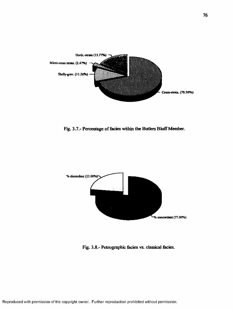
Fig. 3.7.- Percentage of facies within the Butlers Bluff Member.

% discordant (23.00%)

concordant (77.00%)

Fig. 3.8.- Petrographic facies vs. classical facies.


77

are typically analogous to facies volumes. This holds true in most cases for the Oyster

deposits except for the Shelly-gravelly Sand Facies. As was pointed out earlier, this

facies forms in the troughs o f cross lamina sets and is therefore a sub-facies of the Cross-

stratified Sand Facies. Therefore, the Shelly-Gravelly Sand facies, which is not

continuous, occurs within strata sets (Fig. 3.9). Strata cosets were identified using the

classification of McKee and Weir (1953) modified by Allen (1963). Criteria used to

identify cosets include set grouping, set thickness, strata shape and the relationship

between strata and the base o f the sets. Also used to identify cosets is the shape of the

lower bounding surface and the degree o f homogeneity o f sediments within individual

strata sets. Based on these parameters, four cosets have been identified in the mapped

exposure of the Butlers Bluff Member.

Coset A

Co set A is located within Tier 1, which is in the upper two meters of the Butlers

Bluff Member. The most dominant feature is the large scale trough cross stratification

formed by migrating dunes. Cross lamina thickness averages 2.58 mm, and has an

average width of 24 cm. Table 3.3 summarizes the average stratal geometry

measurements of Coset A. Individual sets are underlain by scoop shaped erosional

surfaces. Sets comprising coset A are interfingering and grouped with erosional surfaces

that plunge at one end. Cross strata within individual sets in the x plane are curved and

symmetrical, whereas in the z plane they are sinuous. Average dip o f cross lamina is 20

degrees. In this case, the cross strata to base relationship is discordant (Fig. 3.10). The

cross stratification patterns seen in Co set A most closely resemble Allen’s (1963)

description of Pi-cross stratification, with one exception.


78

Stntal Concepts Ficies Concepts

Shelly Gravelly Faeie*

Fig. 3.9.- Mesoscale architecture of the Oyster Site.


79


80

In this case, pebbly lag deposits are found in the troughs o f most sets making the

degree of lit ho logical uniformity heterogeneous rather than the homogeneous nature as

described by Allen for Pi-cross stratification.

Table 3.3.- Summary o f average stratal geometry measurements o f Coset A

Lamina thickness (mm)

Lamina width (cm)

Set thickness (cm) Set width(m)

Mean 2.58 23.89 10.95 4.49

Std. 0.76 8.10 3.48 3.12

Histograms of lamina thickness and lamina width indicate that these parameters are not

normally distributed, and that lamina widths are considerably variable within Coset A

(Fig. 3.11 and 3.12). Examination of histograms for set thickness and width reveal that

thickness is normally distributed but width is not (Figure 3.13 and 3.14). The mean and

standard deviations for set properties also indicates that set width and thickness are quite

variable as well.

Grain size measurements within Co set A indicate that the average sediment is

a medium sand, moderately sorted and negatively skewed. The average gravel content is

2.1%, but is quite variable within and between individual lamina sets (Table 3.4).

Coset B

Coset B which is contained within tier 2 is very similar to Coset A. Co set B is

composed of large scale trough cross stratification with pebbly lag deposits in the

troughs of individual sets. Sets are grouped and interfingering with erosional scooped


SI

12 - -

10 - -

>>uso3erSb . 6 - -

4 --

2 - -

3.02.0 4.0 5.01.00.0Lamina Thickness (mm)

Fig. 3.11.- Histogram of lamina thickness for Coset A.

12 --------------------------------------------------------------------

10 - -

8 - -

4 -- ---------

2 - -

0 I - i — I | | | f f0.0 5.0 10.0 15.0 20.0 25.0 30.0 35.0 40.0

Lamina Width (cm)

Fig. 3.12.- Histogram of lamina width for Coset A.


Freq

uenc

y

82

15 - -

10 - -

5 --

5.0 10.00.0 15.0 20.0Set Thickness (cm)

Fig. 3.13.- Histogram of set thickness for Coset A.

20

IS

u.

5

0

Fig. 3.14.- Histogram of set width for Co set A.

0.0 2.0 4.0 6.0Set Width (m)

8.0 10.0 12.0


83

shaped surfaces similar to Coset A. Cross lamina dip at 20 degrees like that o f Coset A.

Average set thickness and width for Coset B is not significantly different from Coset A.

Table 3.4.- Textural properties o f Coset A

Mean grain size Sorting (phi) Skewness % Gravel_______________ (phi)_________________________________________________

Mean 1.43 0.84 -1.0 2.1

Std. 032 035 038 3.03

The cross strata to base relationship is also discordant and the degree of lithologic

uniformity is heterogeneous (Fig. 3.15). What is significantly different are the average

lamina thicknesses and widths. Table 3.5 shows that lamina are much more variable in

thickness and width than in Coset A. Coset B probably begins between Tiers 1 and 2,

however we can not see the actual location because tier construction obstructs it.

Table 3.5.- Summary o f the average stratal geometry measurements o f Coset B

Lamina thickness (mm)

Lamina width (cm)

Set thickness (cm) Set width (m)

Mean 4.66 79.77 12.94 539

Std. 3.44 62.95 637 3.03

Histograms of lamina thickness and width indicate non normal distributions and are

similar in shape to the distributions exhibited in Coset A (Fig. 3.16 and 3.17).

Histograms of set thickness and width are also indicative o f non normal distributions

(Fig. 3.18 and 3.19).


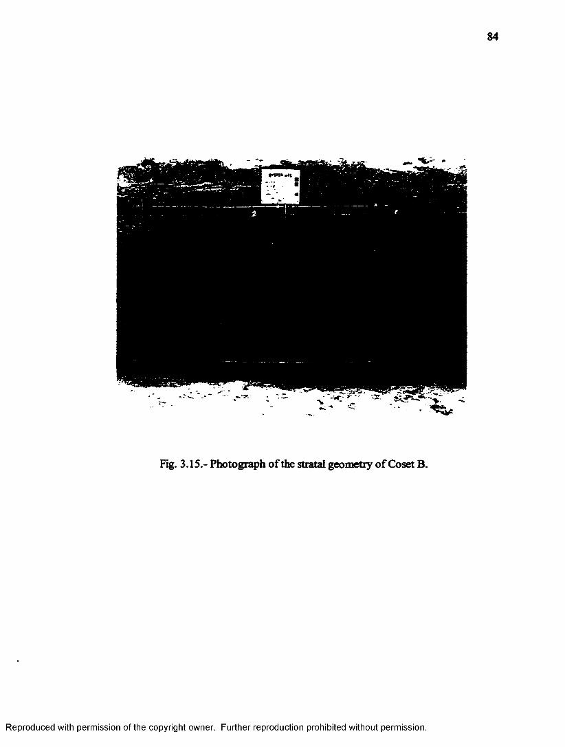
Fig. 3.15.- Photograph of the stratal geometry o f Coset B.


0.0 2.0 4.0 6.0 8.0 10.0 12.0 14.0 16.0 18.0T-amina Thickness (mm)

Fig. 3.16.- Histogram of lamina thickness for Coset B.

20 ---------------------------------------------------------------------------

15 -

5 ■ -

0 *0.0 60.0 120.0 180.0 240.0

Tairnna W idth (cm)

Fig. 3.17.- Histogram of lamina width for Coset B.


8 6

20

IS - -

! 10 - -

0 +0 0 5.0 10.0 iss> 20.0

Set Tbiefciiea (era)2S-0 30j0 35.0

Fig. 3.18.- Histogram of set thickness for Co set B.

s --

rb. 4 - -

2 - -

0.0 10.06.0 12.04.0 14.0 16.0 18.0

Fig. 3.19.- Histogram of set width for Co set B.


87

Average values o f textural properties for Coset B are also significantly different from

those of Coset A. Grain size measurements indicate that on the average, deposits are a

medium sand but the actual mean grain size of 1.7 phi is significantly different than

the mean grain size of Coset A. Sediments in Coset B are better sorted than those in A,

but are still classified as moderately sorted. The gravel content and distribution is quite

similar to that o f Coset A. Table 3.6 summarizes the textural properties of Coset B.

Table 3.6.- Summary o f textural properties for Coset B

Mean grain size Sorting Skewness % Gravel____________________(phO___________________________________________________

Mean 1.70 0.69 -0.66 1.93

Std. 0.45 034 1.03 3.73

Coset C

Coset C is extremely different from Cosets A and B, for it is composed entirely

of parallel to nearly horizontally stratified sediments and thus contains the Horizontally

stratified sand facies. Coset C is located in the lower part of the second tier exposed at

the Oyster Site down to the middle section o f the third tier. This constitutes the lower

part of the butlers Bluff Member (Fig. 3.20). Individual lamina can barely be seen by

heavy mineral contrasts, but could not be measured for thickness. Lamina widths are

most likely continuous throughout the entire width o f individual sets. Sets of Coset C

are differentiated by grain size and color contrasts. Sets are much thicker and wider for

this coset than either Coset A or B, but show a significant amount o f variability (Table


Fig. 3.20.- Photomosaic of Coset C, illustrating parallel laminations and set breaks.


89

3.7). Lower bounding surfaces are non erosional, and fithology within a set is for the

most part is homogeneous. The greater than sign for average set width must be

inchided in the measurements because many sets of Coset C are continuous in width for

the entire exposure.

Table 3.7.- Summary o f stratal geometry measurements fo r Coset C

Lamina thickness Lamina width Set thickness (cm) Set width(mm) (cm) (m)

Mean N/A N/A 39.20 > 8.0

Std. N/A N/A 18.20 >7.0

Set thickness and set width histograms reveal non normal distributions. The primary

set thickness mode is 45 cm, and the primary set width mode is 5 m (Fig. 3.21 and 3.22).

Iron oxide staining also occurs throughout this coset.

Grain size measurements within Coset C show that the sediments are fine grained

sands with the best sorting in the entire Butlers Bluff Member. These well sorted sands

are negatively skewed and have a patchy gravel distribution which is also not normally

distributed (Table 3.8).

Coset D

Coset D is located in the bottom most section o f the Butlers Bluff Member, and

was the least exposed of the four cosets. Co set D contains the Micro-cross stratified

sand facies, and is recognizable by its significant grain size change and color from the

overlying horizontally stratified deposits o f Co set C.


0.00 15.00 30.00 45.00 60.00 75.00Set Thicknes (cm)

Fig. 3.21.- Histogram of set thickness for Coset C.

Oaoscro

0 0 0 5 .0 0 10.00 1 5 .0 0 20 .0 0 25 .0 0Set Width (m)

Fig. 3.22.- Histogram of set width for Coset C.


91

Coset D also contains the curious wavy bedding that is found in Tier 3 (Fig. 3.23). The

bottom section of Coset D exposed in Tier 3 is very close to the water table, therefore

the wavy pattern seen is most likely due to post depositional diagenic processes. Cross

lamina occur throughout the entire coset but in many cases were difficult to see. Lamina

that were measured for their stratal characteristics reveal similarities with cross lamina of

Coset B.

Table 3.8.- Textural properties o f Coset C

Mean grain size Sorting (phi) Skewness % Gravel

Mean 235 0.46 -132 0.43

Std. 031 0.18 1.42 136

The average cross lamina thickness is 4.5 mm, and the average cross lamina width

is 11.74 cm. Set thickness for Coset D does not appear to be significantly different from

average set thicknesses o f Co sets A and B. However, average set width for this coset is

significantly different from the other three cosets of the Butlers Bluff Member (Table

3.9). Also, another difference between Cosets D and B are the average cross lamina dip

angles of 10 degrees instead of 20. Examination of histograms of set thickness and

width indicate non normal distributions of these stratal properties (Fig. 3.24 and 3.25).

Histograms of lamina thickness and width were not constructed due to the low number

of samples taken.

Textural properties measured in Coset D clearly illustrate the similarity of this

coset with that of Coset B.


Fig. 3.23.- Photograph illustrating the break between Cosets C and D, and the general characteristics of Coset D.


Freq

uenc

y

0.00 2.00 4.00 6.00 8.00 10.00 12.00 14.00 16.00 18.00 20.00 22.00SetThidn>eg(cp)

Fig. 3.24.- Histogram of set thickness for Coset D.

us - -

2 - -

L5--

1 - -

0 J - -

2.0 10.0 12.0 14.0 16.0 18.0 20.0Set Width (m)

4.02.00.0

Fig. 3.25.- Histogram of set width for Coset D.

24.00


94

Table 3.9.- Summary o f stratal geometry measurements fo r Coset D

Lamina thickness Lamina width Set thickness (cm) Set width(mm) (cm) (m)

Mean 4.50 73.00 11.74 >14.10

Std. 0.50 6.00 4.84 > 7.35

Sediments in Coset D are generally medium grained, moderately sorted sands. The

sediments appear to be positively skewed, but this may be due to the small sample size (n

= 20) in this coset. The patchy gravel distribution is also similar to that of Coset B

(Table 3.10).

Table 3.10.- Textural properties o f Coset D

Mean grain size Sorting (phi) Skewness % Gravel____________________ (phj)_________________________________________________

Mean 1.65 0.68 0.23 1.85

Std. 0.53 0.12 1.03 2.52

VERTICAL PATTERNS

Set Thickness

Set thickness within cosets tends to be quite variable, however there is an overall

pattern that one can see from the Lower Butlers Bluff section upwards to the Upper

Butlers Bluff section (Coset C to Coset A). Plots o f set thickness vs. elevation were

constructed for various eastings across the Oyster Pit exposures. Close examination of

these plots suggest that set thickness decreases from the Lower Butlers Bluff Member up


95

through the Upper Butlers Bluff Member (Fig. 3.26 through 3.30). This pattern does

not hold true for Coset D, since it has very similar stratal patterns to that of Coset B.

Coset D may actually represent an earlier stage of spit progradation across the

Chesapeake Bay. Allen (1988) points out that as water depth increases, the height and

wavelength of sandwaves increases. As a result, preserved cross strata sets also increase

in scale. If this is true for sandwaves, then it must also hold true for dunes as well since

the only difference between them is scale. In the Butlers Bluff Member, set thickness

decreases upwards, indicating that the depth must be decreasing. This pattern supports

the idea that the Butlers BluffMember represents the progradation of the Nassawadox

Spit across the ancestral Chesapeake Bay.

Grain Size

The general textural pattern that exists within the Butlers Bluff member is that of

a coarsening upwards sequence. This coarsening upwards sequence is indicative of a

prograding shoreline, and can be seen in plots constructed of mean grain size vs.

elevation for various easting along the Oyster Pit exposures (Fig. 3.31 through 3.33).

Fig. 3.34 shows a weak but significant inverse linear relationship between elevation and

mean grain size. This also illustrates the coarsening upward trend. The R2 is only .26,

but the T ratio is 12.39 which is much higher than the critical T value (6.31) necessary

for significance at the 95 % confidence interval.

Close inspection of Fig. 3.31 through 3.33 also indicates that there is a weak but

significant fining upwards pattern of grain size within individual sets. In order to test if

this fining upward sequence occurs from the base o f the trough to the top of individual

sets, grain size data locations were given a new vertical position.


96

586556536855

**610)co 40

49 71

8 31

3 2

Coset Break

0.4 0.50.3 0.60.20.10Thickness (m)

Fig. 3.26.- Vertical pattern of set thickness for easting 964.


Set#

97

66

68 -

72 --

0.2 0.3 0.4 0.5 0.60.10

Coset Break

Thickness (m)



Set#

98

56

68

72

14

0.2 0.3 0.4 0.5 0.60.10Thickness (m)

Coset Break



99

252259645661

=*71<DCO 31

83031 28 142

0.5 0.60.40.30.20.10Thickness (m)

Coset Break



Set#

100

2522

596428

318

3028142

0.2 0.3 0.4 0.5 0.60.10

Coset Break

Thickness (m)



101

Vertical positions assigned were based on height from the base o f the trough for a

particular set. All data points were assigned a value between zero and one. Data points

assigned a value of zero lie at the base of set troughs, whereas those data points that

were assigned a value of one are located at set tops. This new vertical position will be

called set position. Only seven sets contained a sufficient amount o f grain size data

points to test the hypothesis that grain size is correlated to set position. Table 3.11

summarizes the results of the Student’s T-test used for significance testing of this

hypothesis.

Table 3.11.- Results o f significance tests fo r correlation between set position and meangrain size

Set# Student t Critical t ConfidenceLevel

P>t # Data Points

65 2.05 1.00 75 <0.048 36

61 39 1.00 75 0.698 36

59 134 1.00 75 0.199 17

56 239 1.00 75 <0.014 36

3 525 3.08 90 <0.0001 24

14 2.78 1.00 75 <0.0067 86

8 5.05 3.08 90 <0.007 6

From Table 3.11, it is clear that set position and mean grain size are correlated for sets

65, 59, 56, 3, 14 and 8. Most are only correlated at the 75 % confidence interval, and

Set 61 does not indicate a significant correlation between grain size and set position at

alL. O f the six sets that did show a significant correlation, three indicate a coarsening

upwards pattern, and three show a fining upwards pattern.


102

6.5

6 - - Coset A

E,

1 5 . 5 -CO

LLi

Coset B

Coset C4.5 - -

2 2.5 31.510.50

S et Break

Coset Break

Grain Size (phi)

Fig. 3.31.- Vertical distribution of mean grain size for easting 965.3.


Elev

ation

(m

)

103

6.5 -

6 - Coset A

Coset B5.5 -

Set BreakCoset C4.5 - -

Coset Break

1 2 31 0Grain Size (phi)

Fig. 3.32.- Vertical distribution of mean grain size for easting 966.


Elev

ation

(m

)

104

6.5 -

6 - - Coset A

5.5 - Coset B

Set Break4.5

Coset CCoset Break

1.5 2.5 3210.50Grain Size (phi)

Fig. 3.33.- Vertical distribution of mean grain size for easting 968.


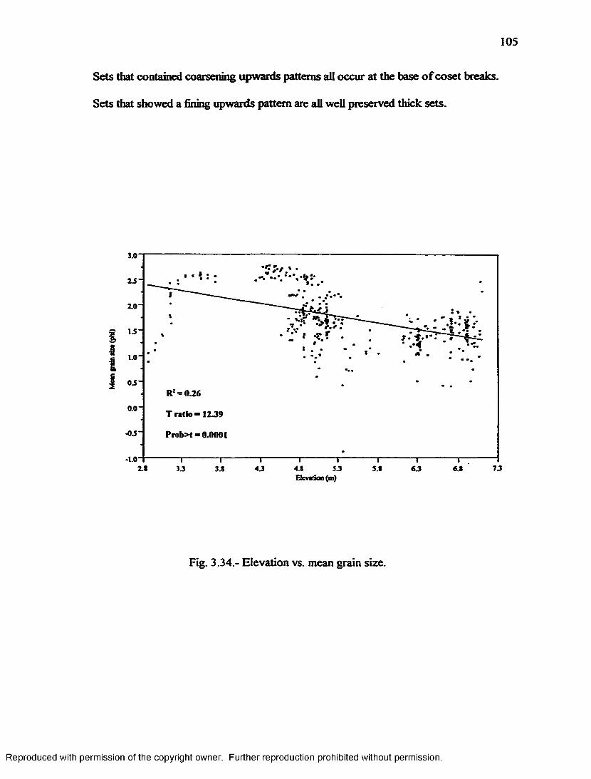
105

Sets that contained coarsening upwards patterns all occur at the base o f coset breaks.

Sets that showed a fining upwards pattern are all well preserved thick sets.

3.0

s u : . r r

i0.0 -

T ratio = 1 2 J9

Prob>t = 0.0001

- 1.07 J2.8 3J 4.8 S3 S.8 6 33.8

Elevation (m)

Fig. 3.34.- Elevation vs. mean grain size.


106

CHAPTER IV

GEOSTATISTICAL ANALYSIS OF THE OYSTER SITE

INTRODUCTION

The term geostatistics refers to a group of powerful techniques used to

understand the nature of spatial data. This chapter examines the spatial nature o f grain

size and permeability in relation to the stratal architecture of the Oyster Site. This

chapter also investigates the scales of stratigraphic organization at which significant

variation exists in grain size and permeability. The techniques used to interpret patterns

of grain size and permeability within a stratal architectural framework include classical

bi-variate plots used by sedimentologists and rigorous statistical one-way analysis of

variance methods. Standardized variograms are constructed to determine correlation

length scales and the Tukey-Kramer Means Comparisons Test is used to determine if

there are significant differences between cosets as well as individual sets for grain size

and permeability. Before any of these techniques could be applied, it was necessary to

construct detailed maps of the stratal architecture with the locations of grain size and

permeability data points included. This allowed for the identification of data points

within cosets as well as individual sets of a particular coset. The methods used to

construct the architectural maps are discussed in Chapter II.

STRATAL ARCHITECTURAL MAPS

Individual sets were mapped within each coset based on the identification of

erosional bounding surfaces and lamina geometry. In the case o f Coset C, individual sets

were recognized by textural and color contrasts as stated earlier in Chapter HI. Often

times, set boundaries were highlighted by iron oxide staining. Sets were numbered


107

sequentially from the base of each coset bottom to top. Each set is designated with an S

for surface followed by the number.

Coset A

This coset occurs at the top two meters of the Oyster Site, between 6 and 8

meters above sea level, and is completely contained within tier 1 of the Oyster Site. A

total of 64 sets have been identified and mapped within Coset A. Although 20 meters

horizontally were exposed within this coset, most samples were collected within an 8

meter distance concentrated mainly in the middle o f tier 1. Fig. 4.1 is an interpretation of

the stratal architecture of Co set A. Thick dark lines indicate set boundaries, and lamina

within sets were drawn to illustrate lamina geometry. Each set contains a unique number

as indicated on Fig. 4.1.

Distribution o f Grain Size Samples. O f the 444 grain size samples collected at

Oyster, 163 were contained in coset A. Table 4.1 is a tabulation of the grain size set

statistics for oset A. Measurements of grain size were obtained from 15 sets in Co set A.

Distribution o f Permeability Samples. A total of 1094 mini air-permeability

samples were collected throughout the Oyster Site. Co set A contained 352 permeability

samples, located within 19 sets. Table 4.2 is a compilation of averages and standard

deviations of permeability measurements for each set.

Coset B

Coset B is located entirely within the upper two-thirds o f tier 2 in the Oyster

Site. This coset is 20 meters long but is not as thick as Co set A. Co set B ranges from

approximately 5.8 meters to 4.8 meters above sea leveL Since Coset B is not as thick as

coset A, it is composed of far less sets.


108

e8


Fig.

4.1

Stra

tal a

rchi

tectu

re

of the

Oy

ster

Site:

Cos

et A.

109

Table 4.1.- Coset A: grain size set statistics

Set# Meangrainsue

Grain size deviation

Sotting Sottingdeviation

Skewness Skewnessdeviation

%Gravel

% Gravel deviation

S22 1.69 032 0.83 031 -1.43 034 236 231

S25 1.44 033 0.90 032 -1.44 039 332 33!

S3! 136 0.15 1.18 0.086 -0.922 0.17 5.03 1.98

S40 1.71 0.034 0.72 0.14 -132 0.40 135 031

S55 1.45 0.00 0.638 0.00 -030 0.00 038 0.00

S 36 1.61 0.15 0.66 0.15 -0.60 0.45 038 039

S59 1-35 032 0.99 038 -0.81 035 4.00 5.02

S 61 132 032 0.91 034 -0.95 030 2.49 2.43

S 64 0.45 0.00 135 0.00 -0.08 0.00 16.74 0.00

S6S 1.45 035 0.84 032 -1.41 0.68 1.63 1.64

S 66 135 0.00 0.79 0.00 -0.95 0.00 034 0.00

S68 1.48 0.05 0.77 036 -0.89 033 1.01 0.76

S69 132 0.18 0.81 0.13 -0.94 0.08 1.40 0.82

S 71 135 032 034 030 -1.03 034 335 3.67

S 72 135 0.03 035 0.04 -0.78 0.17 236 0.76


110

Table 4.2.- Permeability set statistics: Coset A

Set ft Mean Permeability Standard Deviation

(darcys)

S3 32.80 0.00

S22 37.48 11.05

S2S 53.79 19.16

S3I 1932 5.03

S35 4130 1.10

S40 26.80 10.14

S43 34.13 1230

SS3 38.40 0.00

S55 18.10 0.00

S56 32.71 11.42

S59 34.08 4.70

S6I 30.41 12.16

S64 33.88 11.67

S63 4139 1035

S66 17.70 0.00

S68 30.16 8.82

S69 1936 8.40

S7I 30.80 9.61

S72 27.00 13.85


Ill

A total of 28 sets were identified within this coset. Most of the samples collected form

this coset occurred between eastings 964 and 972. Fig. 4.2 is an interpretation of the

stratal architecture o f Coset B and includes the upper part of Coset C.

Distribution o f Grain Size Samples. The number of grain size samples collected

in Coset B equaled 198. Since there were less sets in Coset B, more sets were samples

for grain size than in Coset A. A total o f 12 sets of the 28 identified in Coset B was

sampled for grain size characteristics. Table 4.3 summarizes the textural characteristics

of each set.

Distribution o f Permeability Samples. A total of 19 sets were sampled for

permeability. Mini air-permeameter measurements are foster than grain size analysis

since they are taken directly in the field, therefore many more of these samples could be

taken.. Almost every set was sampled for permeability with 487 individual

measurements throughout this coset. Most sets in Coset B contained numerous

measurements of permeability. Table 4.4 is a tabulation of the average p erm eab ility and

standard deviations for each set in Coset B.

Coset C

Coset C begins at the bottom o f tier 2, just below 5 meters above sea leveL Fig.

4.2 shows the stratal architecture o f the upper part of Coset C, and Fig. 4.3 illustrates

the architecture of the lower part. Since Coset C contains much thicker sets than A or

B, for less sets comprise this coset. Only 6 sets exist within Coset C, all of which are

composed of parallel laminations.

Distribution o f Gram Size Samples. From coset C, a total of 73 grain size

samples were collected.


CoactCCnaetD

( u |N i) a g |p u a

ao001 I

I • •

S3 2 S


Fig.

4.3.-

Stra

tal a

rchi

tectu

re

of the

Oy

ster

Site:

Cos

et C

and

D.

114

Table 4.3. - Coset B: grain size set statistics

Set*

Mean grain size

Gram size deviation

Sorting Sortingdeviation


%Gravel

% Gravel deviation

S3 1.73 0.63 1.03 0.48 -1.71 0.86 4.04 4.48

S4 231 0.05 032 0.02 1.14 0.07 0.00 0.00

SS 221 0.03 039 0.00 0.80 0.18 0.00 0.00

S6 0.80 0.13 138 0.16 -1.05 0.01 8.02 1.80

S8 1.17 0.78 0.94 036 -1.02 1.15 4.10 2.68

S 14 1.79 032 038 035 -032 0.98 131 3.64

S 17 1.06 0.00 1.09 0.00 -034 0.00 18.81 0.00

S 18 1.20 0.88 0.96 032 -030 0.10 5.96 0.41

S 21 0.86 0.63 037 0.42 -0.41 032 4.95 633

S 28 1.74 0.18 037 033 -0.91 0.61 0.60 0.63

S30 1.73 0.18 0.60 0.08 -0.67 038 1.13 1.12

S 31 1.55 0.24 0.68 032 -0.87 0.63 1.14 1.84


115

Table 4.4.- Permeability set statistics: Coset B

Set# Mean Permeability (darcys) Standard Deviation

S3 31.22 24.63

S4 0.01 0.00

S5 0.00 0.00

S6 0.00 0.00

S 7 0.00 0.00

S 8 56.83 20.84

S 11 4623 9.01

S 12 60.82 33.99

S 13 46.10 0.00

S 14 46.51 17.69

S 15 31.18 15.06

S 16 3137 3.13

S 17 53.49 15.90

S 18 6320 15.02

S21 78.40 24.06

S22 56.43 1328

S28 38.87 7.81

S 30 48.15 9.00

S 31 4328 16.93


116

Grain size samples collected came from 4 o f the 6 sets that compose Coset C. Table 4.5

tabulates the grain size statistics for each set.

Distribution o f Permeability Samples. Permeability samples collected from this

coset equaled 234. Every set except for 2 were sampled, giving excellent coverage

throughout this coset. Table 4.6 tabulates the permeability set statistics for Coset C.

Table 4.5.- Coset C: grain size set statistics

Set# Monpan size

Gam size deviation

Sating Satingdeviation

Skewnes Skeunessdeviatioi

% Gravel % Gravel deviation

S I 2.54 003 0.42 058 0.18 031 0.00 0.00

S2 262 0.15 0.43 0.15 -1.47 1.72 035 0.76

S5 243 0.29 0.54 0.22 -1.36 032 139 262

S6 1.46 1.27 0.20 0.17 -0.65 0.65 031 0.48

Table 4.6.- Permeability set statistics: Coset C

Set# Mean permeability (darcys) Standard deviation

S 1 0.00 0.00

S 2 1836 734

S 5 2438 5.63

S6 26.4 6.43

Coset D

Coset D was the least exposed of the 4 cosets as was pointed out in Chapter HI,

therefore only a small number of samples were collected in this coset. Only four sets

were identified within Coset D, with samples taken for grain size and permeability in 3 of

the sets. Fig. 4.3 illustrates the architecture o f this coset.


117

Distribution o f Grain Size Samples. Only 11 grain size samples were collected

in this coset. Table 4.7 shows the grain size set statistics.

Table 4.7.- Coset D: grain size set statistics

Set# M engamsize

Grain size deviation

Sating S atngdeviation


% Gravel % Gravel deviation

S2 1.08 0.13 0.73 0.07 120 0.14 337 321

S3 1.42 a u 0.48 0.04 41.82 042 I3S 132

S4 219 0.21 0.72 0.09 41.82 0.42 138 132

Distribution o f Permeability Samples. Of the 1094 permeability samples

collected in the Oyster Site, only 20 are from coset D. Table 4.8 gives the permeability

set statistics for coset D.

Table 4.8. Permeability set statistics: Coset DB ^ ^ B S B B a a i B ^ B a a a B B B S a S S S a B a S B B S B n B B E B

Set if _ Mean Permeability (darcys) Standard deviation

S 2 90.53 20.69

S 3 62.03 3.88

S4 17.12 9.24

BIVARIATE STATISTICS

General

Bivariate plots have been used in sedimentology for several decades in order to

discriminate between depositional environments. Several authors have attempted to use

these techniques, most notably Folk and Ward (1957); Passega (1964, 1977); Friedman


1 1 8

(1967); Cronan (1972); and McCammon (1976) all of which have met with varying

success. The idea behind the construction o f such plots is that clustering or trends in the

data points are indicative of transport process and therefore depositional environments.

Several bivariate plots were constructed in order to see if any such patterns exist in the

Oyster Site, and if a physical process could be attributed to them. The plots constructed

include mean grain size vs. sorting, skewness and % gravel, sorting vs. skewness, sorting

vs. % gravel, mean grain size vs. permeability and sorting vs. permeability. The

relationship between set thickness and mean grain size was also investigated.

Textural Properties

Mean Grain Size vs. Sorting. The first bivariate plot constructed was that of

mean grain size vs. sorting. Fig. 4.4 clearly illustrates that a good, significant positive

linear relationship exists between these two textural parameters for the Oyster Site. The

R 2 is 0.56, and the t ratio is 23.75, which shows that the relationship is significant at the

99 % confidence level. Also evident is the segregation of the Horizontally stratified sand

facies from the other facies. This is a strong indication that the progressive sorting

process is at work in this depositional system. The plot also suggests that the Shelly

gravelly sand facies is most likely a sub-facies o f the Cross-stratified sand facies.

Mean Grain Size vs. Skewness. Mean grain size vs. skewness is shown in Fig.

4.5, and indicates that there is no clear pattern or relationship between these two

variables at this site. Most samples are negatively skewed, although there is a small

segregation of the Micro cross-stratified sand facies samples. Samples from this facies

are positively skewed, however, as was pointed out in Chapter III, this is may be due to

the small sample size rather than an indication o f a depositional environmental


Reproduced

with perm

ission of the

copyright ow

ner. Further

reproduction prohibited

without

permission.

R square = 0.56

X = Cross stratified sand Facies * = Micro cross stratified sand Facies Y = Shelly gravelly sand Facies Z = Horizontally stratified sand Facies

Mean GralrfSize (phi) * 3.00

Fig. 4.4.- Mean grain size vs. sorting.

120

discriminator.

Mean Grain Size vs. Percent GraveL The relationship between mean grain size

and % gravel is illustrated in Fig. 4.6. The best curve fit for these two variables is a

second order polynomial curve. A second order polynomial curve can also be fit to these

variables. This plot demonstrates that the horizontally stratified sand fecks contains the

least amount of gravel, whereas the gravel percentage is quite variable in the other three

facies. Although the positive correlation suggested by Fig. 4.6 is moderate with an R2 of

0.36, it is significant at the 95% confidence level (t ratio = 9.88). The relationship

shown between grain size and % gravel is also indicative of the progressive sorting

process.

Sorting vs. Percent GraveL The relationship between sorting and % gravel is

strong with an R2 of 0.66 (Fig. 4.7). A second order polynomial curve can also be fit to

this data, which shows that as sorting becomes poorer the gravel concentration

increases. This feet will become very important to the understanding o f the permeability

distribution within a stratal architectural framework. This plot also demonstrates the

segregation of the horizontally stratified sand facies indicating progressive sorting down

the shelf.

Mean Grain Size vs. Permeability. The bivariate plot of mean grain size vs.

permeability reveals a weak positive linear relationship between these two variables (Fig.

4.8). The R2 is only .23, but the t-ratio is 11.44 indicating a significant relationship at the

95 % confidence leveL The plot also clearly illustrates the segregation o f the

horizontally stratified sand facies samples from the other fecks. The horizontally

stratified sand fecies samples tend to have the grain sizes in the fine sand range and


% G

rave

l

-3"

■4'

-S'

x -C n n Stratified Saad Facies A * Micro Cross Stratified S ad Facies Y - Shefly-GravettY Sod Facies Z - Horaoouify Crass Stratified Sm d F«

t

' 1 « 1 ■ 1 ' 1 1—-1.00 -0.50 .00 5 0 1.00 150

Mean Grain Size (phi)2.00

i250 3.00

Fig. 4.5.- Mean grain size vs. skewness.

Fig. 4.6.- Mean grain size vs. % gravel.


Perm

eabilit

y (d

arcys

)

122

25*

20*

15*

10*

X 11 C rass stratified sand Facies • “ M icro cross stratified sand Facies Y “ SW Iy greveffy sand Facies Z 9 H orizontally stratified an d Facies

2351.75.75.25Sotting (phi)

Fig. 4.7.- Sorting vs. % gravel.

140.00

100.00*

80.00**2^ «sr *‘ a V l &* jr fc ,?60.00*

40.00*

20.00* 'X zi

0.003.002.00.00 JO 1.00-1.00

Mean grain size (phi)

Fig.4.8.- Mean grain size vs. permeability.


123

Sorting vs. Permeability. Fig. 4.9 shows an extremely weak, almost no

relationship between sorting and permeability. The R2 is 0.05, and the t-ratio is not

significant at the 95% confidence level. This plot does show that the horizontally

stratified sand facies has the best sorting and the lowest overall permeability.

Mean Grain Size vs. Set Thickness. The relationship between mean grain size

and set thickness was investigated at the Oyster Site. Fig. 4.10 indicates that a good

parabolic relationship exists between these paired variables. The R2 is 0.52, and the

correlation is significant at the 99 % confidence interval. The parabolic relationship

suggests that the coarsest and the finest grain sizes tend to have the thickest sets

preserved. An important feature to note is the minimum that exists at 1.5 phi (0.35 mm).

ANALYSIS OF VARIANCE RESULTS

General

Analysis of variance tests ( ANOVA) are statistical tests that allow the total

variation of a data set to be segregated into its parts. The analysis of variance test is

designed to compare the individual variances that make up the total variance. In doing

this, one is able to test the statistical significance of the observations. The method in

which one-way ANOVAS are calculated is discussed in Chapter II. However, as I

mentioned earlier in Chapter II, I will discuss the assumptions of the ANOVA tests in this

section. I will also explain the Tukey-Kramer Means Comparison Test that was used

after the analysis of variance tests were performed (Krumbein and Miller 1953).

Three main assumptions should be met before undergoing such an analysis. The

first assumption is that no significant interactions occur between observations.


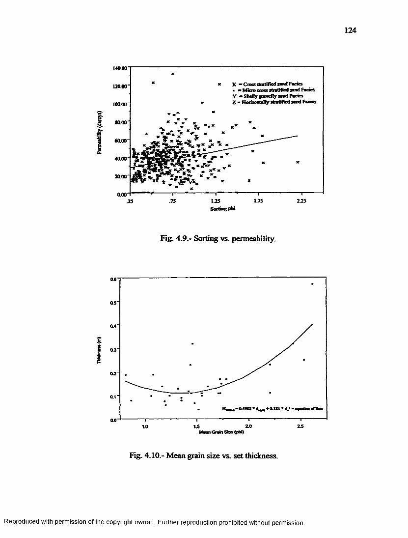
124

140.00 '

120.00

100.00

*0.001

60.00

40.001

20.00

0.00

* X - Cross stratified sand Facies« = Micro cross stratified sand Facies Y ” Shefly gravelly sand F«cics Z “ HotbBataOy stratified sand Facies

S

^ w

.25—r~.75

1—I tIJ5Sorting phi

I.7S Z25

Fig. 4.9.- Sorting vs. permeability.

0.6

as*

£2 03 "

I

02*

ai*

H - , ,-0 .« 9 0 2 * < l t .„ -t-0 .IS I •< .«

ao2.0 2.5

M ean G ra in S iz e (p h i)

Fig. 4.10.- Mean grain size vs. set thickness.


125

This is also known as the assumption of additivity. For the type of data used in this

study one can assume that there is no interaction between individual data points because

grain size or permeability measurements in one location usually does not affect another.

The second and third assumptions are much more important for most geological data.

Assumption two is that of normality. Each data group should theoretically be normally

distributed, however it has been pointed out that the consequences of non normality are

not serious since the f-ratio is quite robust for moderately skewed data. F-tests break

down and are not valid only when the sample is extremely skewed (Cochran 1947). The

third assumption is known as the homogeneity o f variance. The one-way ANOVA test

generally assumes that the variances between each group are equal. This is probably the

most important assumption because if this condition is not met the ordinary ANOVA test

is invalid. The assumption of normality and homogeneity of variances will be addressed

for each ANOVA run (Krumbein and Miller 1953; Dowdy and Wearden 1991). An

analysis of variance test was conducted first using cosets as the data groups. This was

done to test the null hypothesis that the mean grain size and permeability is not

significantly different between individual cosets. Each coset is then tested for the

hypothesis that individual set means o f grain size and permeability are not significantly

different. These ANOVA tests will aid in the determination of the stratigraphic scales at

which grain size and permeability variability is most important. As an aid to the

understanding of the ANOVA tests, box plots were constructed of the data groups so

that visual comparisons could be made. Fig. 4.11 is an illustration o f a generic box plot

used in this study.


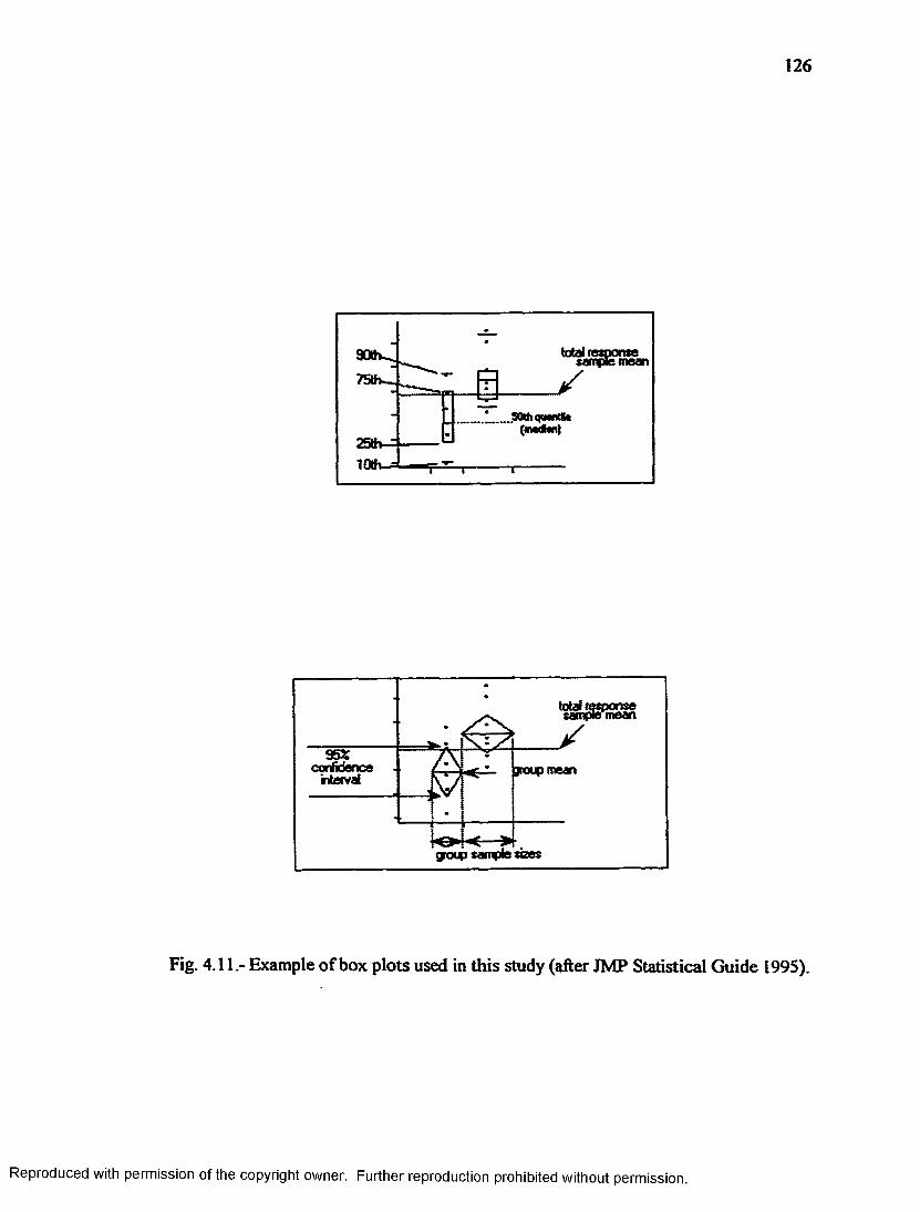
126

total mean

total n mean

953:confidence

intervaljroupmean

groip sample sees

Fig. 4.11.- Example of box plots used in this study (after JMP Statistical Guide 1995).


127

Tukey-Kramer Means Comparision Test

The one-way analysis o f variance test only determines if at least one of the group

means is significantly different. If the null hypothesis is rejected, it would be

advantageous to know which data group or groups were unequal. Several multiple

comparisons test exist which are able to discern which groups are unequal. Some

require the null hypothesis to be rejected first, while others do not. The multiple

comparison test chosen for this study was the modified Tukey’s Honestly Significant

Difference (Dowdy and Wearden 1991; Tukey 1949). All multiple comparison tests

are based on what is known as “The Least Significant Difference.” This is basically a t

test, therefore if all of the data groups are of equal size then two group means can be

tested for a significant difference by the equation below.

\yryM *MS,

2 ------------ -

n (4-1)

In this equation, Mse is the variance of the error or the mean square of the within set

group. The confidence interval chosen for all tests was 95% (a = 0.05). This Least

Squares Difference Test is also known as Fisher’s Test. Tukey’s Honestly Significant

Difference Test was chosen over other tests because o f it’s conservative nature, and the

feet that rejection of the null hypothesis is not required. In this test, the least squared

difference is subtracted from the actual absolute difference in the means for all data pairs.

This reduces the error rate to that o f the confidence interval chosen, and is one of the


128

strictest means comparisons tests, for it uses a single critical difference unlike Fisher’s

Test or others.

M S'n (4-2)

In the statistical equation above, q represents the quantile used to scale the least squared

differences, and is similar to a Student’s t-test (Tukey 1949, 1991; Duncan 1955; Saville

1990; JMP Statistical Guide 1995). Kramer (1956) modified the Tukey Means

Comparison test to include situations where data groups contain unequal sample sizes.

The results of the multiple means comparison test is displayed in both tabular and

graphic form. Once the analysis is run, a table is created that illustrates which data

groups are significantly different from one another. All positive values in the table

indicate significant differences in the means of those data groups. One can also visualize

the results by constructing comparison circle plots. In the circle plot, group means are

represented by a circle. A comparison o f individual group means is done by examining

the intersection of the circles (Fig. 4.12). Group means whose circles intersect at a 90

degree angle or inscribed circles are not significantly different. If the intersection of two

circles are less than 90 degrees or if they do not intersect at all, then the means are

significantly different (JMP Statistical Guide 1995).

Coset Variability

Grain Size. An analysis of variance test was performed first on individual cosets.

The null hypothesis states that coset means are equal. The alternative hypothesis is that


129

angle greater than 90 degrees

not significantly different

angle equal to 90 degrees

border linesignificantlydifferent

angle less than 90 degrees

significantlydifferent

Fig. 4.12.- Definition sketch of means comparison circles (after JMP Statistical Guide 1995).


130

at least one coset mean is unequal. As was stated earlier, the assumption of normality

should be tested for each data group. This was not conducted for grain size data groups

because grain size is usually assumed to be log normality distributed. If this assumption

is not made, then ordinary grain size statistics would be invalid, therefore for the

purposes of grain size only log normality is assumed and the condition of normality for

the ANOVA is met. The F-ratio is also fairly robust for the homogeneity of variances. In

this case, variances are not very different so the conditions for the ordinary one-way

ANOVA were met. Inspection o f the box plot for each coset reveals that the means for

grain size are different (Fig. 4.13). The ANOVA test resulted in an F-Ratio of 148.2,

which far exceeds the critical F-value of 2.60 (Table 4.9). Since the F-Ratio exceeds the

critical value, the null hypothesis must be rejected and the alternative hypothesis is

accepted. The mean square values indicate that the variance among cosets is much

greater than the variance within cosets.

Table 4.9.- ANOVA results fo r grain size o f cosets

Source Degrees o f Freedom Sum o f squares Mean Square F-Rario

Among Cosets 3 62.09 20.70 148.2

Within Cosets 440 61.46 0.14 ------

Total 443 123.57 ------ ------

The Means comparison circles indicate that only coset D is indistinguishable by mean

grain size (Fig. 4.13). Table 4.10 gives the results of the Tukey-Kramer HSD Test.

Results from the Tukey-Kramer Test reveal that coset C has a significantly different

mean grain size from all other cosets, and that the mean grain size of coset D is not


131

oo._4JO

CoU)*cC3Q.£ooWJceaVE

<uN

'55C

'SwCO

Ol4-»_o"S.X0J3<D0 1 OO1

c*i

00

(njd) azjs ukiq oeafy


132

significantly different from cosets A and B.

Table 4.10.- Means comparison results o f cosets: grain size

COSET C B D A

C -0.16 0.72 0.59 0.97

B 0.72 -0.10 -024 0.15

D 0.59 -0.24 -0.41 -0.09

A 0.97 0.15 -0.09 -0.112_58

Both the ANOVA test and the Tukey-Kramer Means Comparison Test prove that

statistically, the coset level exhibits significant control of grain size variability.

Permeability. An ANOVA test was performed to test the null hypothesis that

coset means of permeability are equal Therefore, the alternative hypothesis is that coset

permeability means are not equal First, the assumptions of normality and homogeneity

of variances must be tested. In order to test if individual cosets pass the assumption of

normality, quantile vs. quantile plots (Q-Q plots) were constructed. Plotted on the

abscissa is the standard deviations from the mean, and the permeability values are on the

ordinate. If a variable is normally distributed, then a diagonal line is plotted (Fig. 4.14).

Q-Q plots for each coset illustrate that cosets closely fit the normal distribution and at

the most are only moderately skewed (Fig. 4.15 through 4.18). Variances of each of the

co sets were not extremely different, therefore the assumption of homogeneity of

variances was met. Visual inspection of box plots constructed for mean permeability

values for each coset suggests that a large amount o f variability exists between cosets

(Fig. 4.19).


133

180-f

160-

140-

120-

100-

80-

60-

Normal QuantHe

Fig. 4.14.- Example of the normal quantile plot (after JMP Statistical Guide 1995).

.75SO .90 .9505 .99JOS .K>120“

100“

80“

60“

40“

20 “

0*130 2I I-2-3

Normal Quantile

Fig. 4.15.- Q-Q plot: Coset A.


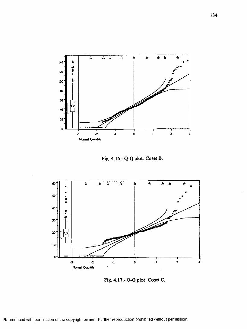
90 95.75JO05

120*

100*

60*o

40"

20"

0*12 3I0-2 -t-3

Normal Quantile

Fig. 4.16.- Q-Q plot: Coset B.

95.75 995005 .1001

40"

3 0 '

20"

10*

0"<321-2 0■3 I

Normal Quantile

Fig. 4.17.- Q-Q plot: Coset C.


135

.75 .90 95 .99.1005

125"

100'

75"

50"

25"pOO

21 30-1•3 ■2Normal Quantile

Fig 4.18.- Q-Q plot: Coset D.

I«0"

120"

100"

f

lCL.

20 "

Coset0.05

Fig. 4.19.- Coset box plots and means comparison circles of permeability.


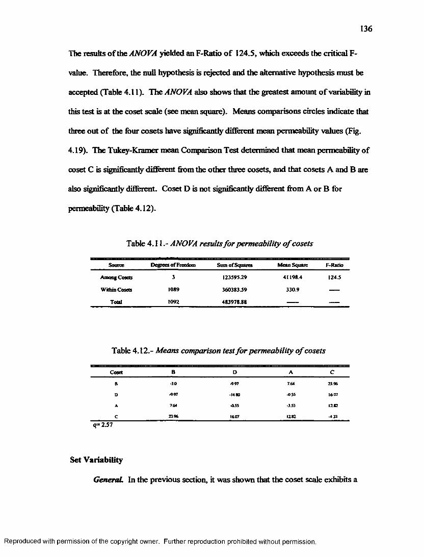
136

The results of the ANOVA yielded an F-Ratio o f 124.5, which exceeds the critical F-

value. Therefore, the null hypothesis is rejected and the alternative hypothesis must be

accepted (Table 4.11). The ANOVA also shows that the greatest amount of variability in

this test is at the coset scale (see mean square). Means comparisons circles indicate that

three out of the four cosets have significantly different mean permeability values (Fig.

4.19). The Tukey-Kramer mean Comparison Test determined that mean permeability of

coset C is significantly different from the other three cosets, and that cosets A and B are

also significantly different. Co set D is not significantly different from A or B for

permeability (Table 4.12).

Table 4.11.- ANOVA results fo r permeability o f cosets

Source Degrees o f Freedom Sum o f Squares Mean Square F-Ratio

AmongCosets 3 123595.29 4II98.4 124.5

Within Cosets 1089 360383.59 330.9 -----

Total 1092 483978.88 ------ -----

Table 4.12.- Means comparison test fo r permeability o f cosets

Coset B D A cB -30 -9.97 764 23 96

D -997 -1480 -055 1607

A 764 -055 -353 1282

C 23 96 1607 12.82 -4 33

q = 2 J 7

Set Variability

GeneraL In the previous section, it was shown that the coset scale exhibits a


137

large amount o f variability in both grain size and permeability, which distinguishes one

coset from another. It was also shown that coset variability makes up more of the total

variability than that o f set variability. In order to determine if set scale variability is

statistically significantly important to grain size and permeability, ANOVAS and means

comparison tests were performed for each coset. The data groups are now the individual

sets, and the assumptions for the one-way ANOVA must be tested for each set group.

Coset A . As was stated earlier, grain size data is assumed to be log normally

distributed, therefore grain size is assumed to pass the assumption of normality.

Permeability set groups were tested for normality by constructing Q-Q plots. Most

groups were either closely normally distributed or only moderately skewed. A small

number of set groups did not pass the normality test and were removed from the ANOVA

test. This occurred in sets with only a few data points. As a general rule, sets that

contained less than 4 data points were omitted from the analysis for both grain size and

permeability. Grain size variances did not differ greatly, therefore the homogeneity of

variances assumption was also met. The assumption of homogeneity of variances also

held true for permeability.

Coset A: Grain Size Results. Set grain size means varied between 1.2

and 1.7 phi. Box plots o f set means indicate that more that one set group is most likely

significantly different (Fig. 4.20). The ANOVA tested the null hypothesis that set grain

size means are all equal. Results of the ANOVA Test yielded an F-Ratio of 2.87, which

exceeds the critical value o f 2.60. The null hypothesis is therefore rejected, and one

must conclude that at least one of the set means for grain size is significantly different.

Table 4.13 shows that the set scale contains more than two-thirds of the total variation in


138

coset A. Means comparison circles indicate that at least three sets have significantly

different grain size means (Fig. 4.20). The Tukey-Kramer Means Comparison Test

reveals that several sets are indeed significantly different to one another with respect to

grain size. Sets 40, 69, and 72 show no significant difference with any other set (Table

4.14). However, these three sets all have the minimum number of observations allowed

in this study.

Table 4.13.- ANOVA results ofgrain size fo r Coset AK a ^ ^ n a n n a B n n B B B B a a B a a B a B ^ ^ B s t a B B m s s s s

Source Degrees of freedom Sum o f squares Mean square F-Ratio

Among Sets 10 226 022 2.87

Within Sets 148 11.65 0.08 ------

Total 158 13.91 ----- ------

All of the other sets are significantly different with more than one other set. The results

of the means comparison test clearly indicate that sufficient variability exists between

individual sets in a coset with respect to grain size. Sets that do not show a significant

difference between mean grain size are typically very thin with significant truncation, as

well as the small number of observations with the largest standard deviations. This result

may be due to the severe truncation of a set by the next set that causes no significant

difference in grain size.

Coset A: Permeability Results. Inspection of set box plots constructed

for permeability indicate that several set means deviate from the grand mean (Fig. 4.21).

The results of the ANOVA test for permeability in this coset produced an F-Ratio of


139

2f

I.S-

I<512 1.0-

i

0 5 -

66 6S65

Set *

Fig. 4.20.- Box plots and means comparison circles of grain size: Coset A.

3

130

120no10090

60

40

All Pain64Set*

0.05

Fig. 4.21.- Box plots and means comparison circle for permeability : Coset A.


140

9.48. Since this F-Ratio exceeds the critical F-vahie, the null hypothesis is rejected and

one is forced to conclude that at least one o f the sets is significantly different from the

grand mean (Table 4.15).

Table 4.14.- Grain size means comparisons results: Coset A

Set# 40 22 56 69 68 65 25 59 71 61 72

40 -0.55 -0.46 -0.30 -031 -0.32 -0.14 -014 -005 -0.08 •0.01 -0.09

22 -0.46 -0.39 -072 -0.25 -027 -0.06 -006 0.03 -0.0! 0.08 -0.03

56 -0J0 •0.22 •0.13 -0.24 -0.26 0.03 0.01 0.10 0.02 0.16 -003

69 -021 -0.25 -0.24 -045 -0.46 -027 •026 -.18 -021 -014 -023

68 -0.32 •0.27 -0.27 -0.46 -055 -028 -028 -029 -032 -025 -022

65 -0.15 -0.06 0.03 -0-27 -0.38 -0.13 -015 -0.06 -0.13 0.00 -0.19

25 -0.14 -006 0.01 -0.26 -038 -0.15 -020 -0.11 -0.17 -0.05 -022

59 -0.05 0.03 0.10 -0.18 -029 -0.06 -0.11 -0.19 -025 -0.13 -022

71 -0.08 -0.01 003 -021 -022 -0.13 -0.17 -025 -022 -022 -025

61 •0.01 0.08 0.16 -0.13 -025 0.00 -0.05 -0.13 -022 -0.13 -0.33

72 -0.09 -0.03 -0.03 -023 -022 -0.19 •022 -031 -025 -023 -0.55

Table 4.15.- ANOVA results for set permeability: Coset A

Source Degrees of Freedom Sam of Squares Mean Square F-Ratio

Among Sea II 17350.15 157729 9.48

Within Sets 331 5505621 16623

Total 342 72406.45 ------- -------

Means comparison circles clearly signify that several sets are significantly different from

one another with respect to permeability (Fig. 4.21). Results o f the Tukey-Kramer

Means comparison test can be found in Table 4.16. The Tukey-Kramer test not only


141

found that several sets are significantly different, but that the differences are much larger

than those for grain size. Clearly the set level is a good predictor of permeability since

one can easily differentiate individual sets from one another with respect to permeability.

Coset B. The assumption o f normality for the permeability data was met, since

sets in this coset were closely normally distributed or only moderately skewed. The

assumption of homogeneity of variances was also met for both grain size and

permeability set groups, therefore the one-way analysis of variance is valid for this coset.

Coset B: Grain Size Results. Inspection o f box plots constructed for

each set indicates that possibly 5 sets are significantly different from the grand mean (Fig.

4.22). The analysis of variance results yielded an F-Ratio of 5.20, which is above the

critical value of 2.11. Therefore, the null hypothesis is rejected and the alternative

hypothesis that at least one set mean for grain size is significantly different is accepted

(Table 4.17). The ANOVA also indicates that over 90% of the total variability is at the

set level in this coset. Means comparison circles also indicate that five sets are

significantly different from one another with respect to grain size. The complete results

of the Tukey-Kramer Means comparison test confirms that indeed 5 out of the 10 sets in

coset B used in this analysis are significantly different from one another (Table 4.18).

Coset B: Permeability Results. Several sets in coset B appear to be

significantly different from the grand mean upon examination of set box plots (Fig. 4.23).

ANOVA results generated an F-Ratio that far exceeded the critical value of 1.81 (Table

4.19). Since the F-Ratio exceeded the critical value, the null hypothesis must be rejected.

Therefore, we know that at least one set is significantly different from the others

with respect to permeability. Means comparisons circles illustrate that many sets are


Table

4.

16.-

Mea

ns

com

paris

on

resu

lts f

or p

erm

eabi

lity:

Cos

et A

142

o \ o or4 3a •5

.20 a

9 ■123

3 «s9 •9

.49

•896

•160

5 s

-268

5

40

5! 5»r4

S♦ £ ?N

S 8ooX•O 3 •3

0.02

-210

4

00 s« R•f

R2 8 3

•23.

13 8!g

•202

9 ££ S8

r«

33

opm

f-«

8m « X£ <ri

9© •o

82*

X«o 8

hp 3

of?9

s 89

R 3r -

3<•» ©

88

8 9<?'

56 3

H a 89

89

89

s9

SP-- «r\«n

82

8Wk

m■9

SN9

?N 8«0

Ses

mp»£ •2

615 8

«o«P»r»

Xo

«n3

8 m«

Os*r% S«o

ooci

r«-©

r*<Ar« S8

S9

8 Rp»

3r- Rwi 3•9

oK>♦ •o s

«mf—© R

as S9

3C-2w>

8« R 8•rt

<N r» S«o

X 8oo © 8

m 89

81-̂ 8<A8 «

OOn

SO £(S*•9

89

«r> «*\♦9 « 3 so

P-n

R•f

8 8r<

W-i<N

so e

m m ©m«o

M9 «*t

np» p»m S

Ofeo

CO

«r»CM «oo

M e n O'to N©

v©«o r-* NO

ooo

O 9 s>©


143

2.5"

Is

V )

i3s

10'

0 0 '

S e t t0.05

Fig. 4.22.- Box plots and means comparison circles of grain size: Coset B.

10 II 12 14 15 17 It 21 22 2* 30 31Sctf

All Pnrs

Fig. 4.23.- Box plots and means comparison circles o f permeability: Coset B.


144

Table 4 .17.- ANOVA results fo r grain size: Coset B

Source Degrees o f freedom Sum o f Squares M en Square F-Ratio

Among Sets 9 7.51 0.83 5.20

Within Sets 181 29.02 0.16

Total 190 36.53

Table 4.18.- Means comparison results fo r grain size: CosetB

Set#

7 14 3 28 30 31 21 8 18 17

7 474 404 407 417 419 014 404 042 018 416

14 404 419 427 446 448 400 441 0.16 416 456

3 407 427 436 4S2 434 414 445 0.09 421 459

28 417 446 452 468 470 436 457 409 434 468

30 419 448 434 470 474 4.41 460 413 437 471

31 014 403 414 436 441 428 463 406 438 477

21 404 441 445 437 4.60 463 -128 491 -1.08 -134

8 042 016 009 409 413 406 491 457 484 -120

18 018 416 421 434 437 438 •1.08 484 -105 -134

17 41S 456 459 469 471 477 -134 -120 -134 -1.81


145

Table 4.19.- ANOVA results ofpermeability: Coset B

Source Degrees of freedom Sum o f Squares Mean Square F-Ratio

Among Sets 14 63524.73 4537.48 12.56

Within Sets 461 166475.15 361.12 -------

Total 475 229999.88 ------- -------

significantly different from one another (Fig. 4.23). Table 4.20 gives the full Tukey-

Kramer results, indicating which sets are significantly different from one another.

Coset C All the assumptions required for the one-way analysis of variance for

grain size were met This was also the case for the permeability data. Coset C contained

a total of 72 observations organized into four sets.

Coset C: Grain Size Results. Box plots constructed for each set

indicate that at least one set group is different from the grand mean with respect to grain

size (Fig. 4.24). ANOVA results produced an F-Ratio of 3.27, which exceeds the critical

value of 2.74 (Table 4.21). Results from the ANOVA test also show that variation is

similar at both the set scale and lamina scale. The null hypothesis must therefore be

rejected. This means that at least one set is significantly different from the other set with

respect to grain size. Means comparison circles indicate that two of the four sets are

significantly different from one another (Fig. 4.24). The full results o f the Tukey-Kramer

Means comparison test can be found in Table 4.22. The Tukey-Kramer test revealed

that set 2 and 5 are the only sets that are significantly different. These two sets have the

most observations, whereas the other two have the minimum number o f observations.

Set 1 has the smallest width, and set 6 is close to the top o f tier 3. Interestingly, set 2 is


146

located beneath coset B and set 5 is located just above coset D.

Coset C: Permeability Results. Set # 1 was omitted from the analysis

due to a low number of observations. Careful examination of box plots reveals that set 2

mean permeability is different than set 5 and 6 (Fig. 4.25). ANOVA results indicate that

the null hypothesis must be rejected, meaning that at least one set mean is statistically

different than the other set with respect to permeability (Table 4.23). Means comparison

circles indicate that two sets in coset C are significantly different with respect to

permeability (Fig. 4.25). Table 4.24 gives the complete results o f the Tukey-Kramer

Means comparison test for permeability in coset C.

Coset D. All of the required conditions for the one-way analysis of variance were

met for both grain size and permeability. Set 1 of this coset was omitted from both the

ANOVA tests due to a low number of observation. A total of 11 observations located in

3 cosets were tested for the null hypothesis that all set means with respect to grain size

and permeability are equal.

Coset D: Grain Size Results. Box plots of the three sets in this coset

indicate the possibility that more than one set is significantly different from the grand

mean (Fig. 4.26). The analysis of variance test yielded a very significant F-Ratio,

therefore the null hypothesis must be rejected (Table 4.25). Means comparison circles

indicate that two of the thee sets are significantly different from each other with respect

to grain size. Table 4.26 gives the results o f the Tukey-Kramer Means comparison test.

This test revealed that set 4 is significantly different from sets 2 and 3, but that sets 2 and

3 are not significantly different from each other. Set 4 happens to be located just below

coset C.


Mea

n Gr

ain

Size

(phi

)

147

u s-2.4 -

2 3 '

2. 1*

S e t*0.0S

Fig. 4.24.- Box plots and means comparison circles of grain size: Coset C.

AH P m

Fig. 4.25.- Box plots and means comparison circles of permeability : Coset C.


Table

4.

20.-

Mea

ns

com

paris

on

resu

lts

of pe

rmea

bilit

y: C

oset

B

148


149

Coset D: Permeability Results. The box plots o f permeability for this

suggest that all three sets are significantly different (Fig. 4.27). Results of the ANOVA

yielded a large F-Ratio, forcing the acceptance o f the alternative hypothesis that at feast

one set mean is significantly different (Table 4.27). Means comparison circles also

indicate that all three sets are significantly different with respect to permeability (Fig.

4.27).

Table 4.21.- ANOVA results o f grain size: Coset C

Source Degrees o f freedom Sum o f Squares Mean Square F-Ratio

Among Sets 3 0.43 0.14 3.27

Within Sets 68 2.99 004 -------

Total 71 3.43 ------- -------

Table 4.22.- Means comparison results o f grain size: Coset C

Set H 2 6 1 5

2 -0.12 -024 -023 0.03

6 -0.24 -029 -027 -0.18

I -0.22 •027 -029 -020

5 0.03 -0.18 -020 -0.17

Table 4.23.- ANOVA results o f permeability: Coset C

Source Degrees o f freedom Sum o f Squares Mean Square F-Ratio

Among Sets 2 133428 66729 1226

Within Sets 227 1205726 53.12 -------

Total 229 13391.84 ------- -------


150

2.5

2.0 "

13V )

1.5*c635

1.0 *

Secf0.05

Fig. 4.26.- Box plots and means comparison circles of grain size: Coset D.

ISO

125“

100-

s3§«*a. JO-

25'

Set*

Fig. 4.27.- Box plots and means comparison circles of permeability: Coset D.


151

Complete results o f the Tukey-Kramer Means Comparison Test is given in Table 4.28.

Table 4.24.- Means comparison results ofpermeability fo r Coset C

Set# 6 5 2

6 -10.02 -5.87 0.99

5 -5.87 -*.92 2.45

2 0.99 2.45 -1.91

Table 4.25.- ANOVA results o f grain size: Coset D

Source Degrees of freedom

Stmt o f Squares Mean Square F-Ratio

Among Sets 2 2.85 1.43 38.69

Within Sets 8 0.29 0.04 ------

Total 10 3.15 ------- ------

Table 4.26.- Means comparison test results o f gram size: Coset D

Set# 4 3 2

4 -035 032 0.74

3 032 -035 •0.14

2 0.74 -0.14 -039

Table 4.27.- ANOVA results o f permeability: Coset D

Source Degrees of freedom

Sum o f Squares Mean Square F-Ratio

Among Secs 2 21845.98 10923.00 5238

Within Sets 17 3552.14 208.90

Total 19 25398.11


152

The results show that indeed all three sets are significantly different with respect to

permeability.

Table 4.28.- Means comparison test results o f permeability: Coset D

Set# 2 3 4

2 -21.41 12% 5459

3 2.28 -V i 2% 20.76

4 54.59 20.78 -15.81

VARIOGRAM RESULTS

General

Variograms were constructed in order to determine the horizontal and vertical

correlation length scales of both grain size and permeability in the Oyster Site. The

reason why such an analysis was done is that the correlation length scales provide

detailed information regarding the spatial continuity o f the properties measured. Once

the correlation length scales have been determined, they can then be compared to the

scales o f stratigraphic organization recognized in the Oyster Site sediments. This will aid

in determination o f the stratigraphic scales of organization that are most important to the

distribution of grain size and permeability. Due to the nature of the data collected,

variograms were constructed for both grain size and permeability for cosets A, B and C.

Coset D data was not included in the variogram analysis because o f the small number of

observations and the lack of spatial coverage in this coset. The general theory behind the

variogram can be found in Chapter II.


153

Before the results of the variogram analysis are discussed, there are a few

preliminary considerations about the construction of variograms that must be addressed.

When constructing a variogram, there are several parameter values that must be chosen

by the user in order to create the most confident variogram. The first parameters are the

x and y coordinates. For this study, the x coordinate is the easting, and the y coordinate

is the elevation. The next parameter is the direction angle. For the horizontal

variogram, the angle is zero, and for the vertical direction the angle is 90 degrees.

Because we know that most data pairs do not lie at exactly at zero or 90 degrees, we

must choose an angular tolerance. This allows for the inclusion of more data pairs in the

analysis. For most of the variograms in this study, an angular tolerance o f 20 degrees

was used. Also important is the lag spacing, lag tolerance, and the number o f lags. The

lag spacing is the distance over which the variogram samples the data set. A good lag

spacing is typically the spacing used in the data acquisition (Isaaks and Srivastava 1989).

In this study, the sampling spacing was approximately 0.2 meters, therefore, for each

variogram the lag spacing was 0.2 or 0.1 meters. Since all the data points were not

taken at exactly this spacing, a lag tolerance of half the lag spacing was chosen. The

number o f lags chosen for each variogram depends on the data itself One wants to get

the most spatial coverage, but too many lags may obscure the structure (Fig. 4.28). AH

of these parameters are carefully chosen to yield the most pairwise data points at the first

lag distances and to produce the most structure. Generally, 20 or more pairwise data

points in the first lag is considered optimal (Isaaks and Srivastava 1989; Davis 1986;

Pannatier 1996).


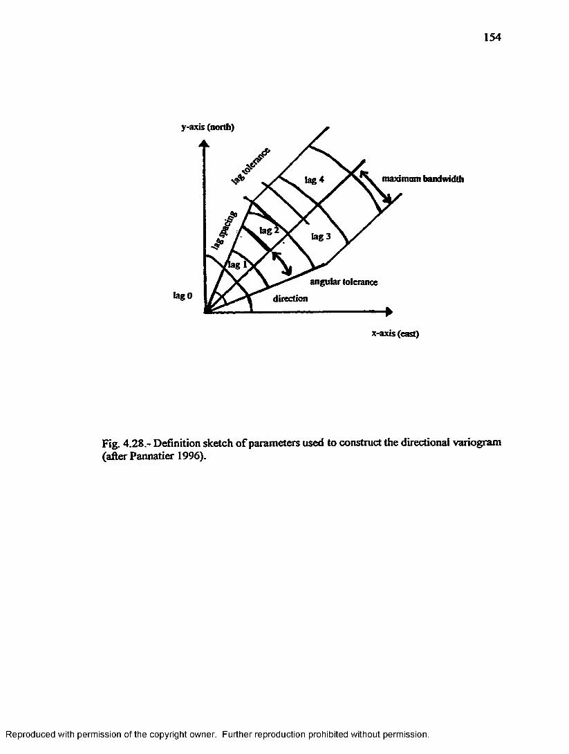
154

y-axis (north)

maximum bandwidth

lag lag 3

angular tolerancelagO direction

x-axis (east)

Fig. 4.28.- Definition sketch of parameters used to construct the directional variogram (after Pannatier 1996).


155

Variogram Modeling

Once an adequate variogram is obtained, one typically fits one o f three common

models in order to determine the correlation length scale. The three common models

used are the exponential, spherical and gaussian. In this study, the spherical model and

the exponential model were used because they fit the variograms welL The spherical

model is defined by equation 4-3 (Pannatier 1986). In equation 4-3, a is the range and c

is the sill value.

T(|A|)=c*^A.(|A|)=c*[1.5-^-0.5M2l] (4 _3 )a a

The spherical model behaves linearly at the origin, until the sill is reached at the range.

The exponential model is also commonly used to model variograms, and is defined by

equation 4-4.

r|A|=c»Sp.l*l=c*[l-« ‘ I ('M)

Coset A

Grain Size Results. The horizontal experimental variogram was calculated using

an exponential model with a lag spacing o f 0.2 meters, and the number o f lags is 15. The

exponential model for horizontal grain size produced a sill value of 0.09 and a range of

0.65 meters (Fig. 4.29). The variogram shows that the correlation length scale occurs at


156

a short distance (0.65 meters), which means that there is lack of extensive spatial

correlation in this direction. Table 4.29 lists the number o f data pairs for each lag

number. The vertical variogram o f grain size shows that there is no discemable range.

This is a pure nugget model at the smallest lag, which suggests a correlation length scale

that is small than the sampling distance (Fig. 4.30). Lag spacing for the variogram was

0.1 meters, and the number o f lags was 5. The resultant variograms indicate that grain

size has a larger correlation length scale in the horizontal direction than in the vertical

direction. Table 4.30 is a list o f the number of data pairs for each lag.

Permeability Results. The horizontal variogram for permeability was calculated

using an exponential model, and shows a similar structure to that of grain size. The

range occurs at 0.87 meters, indicating that both variables are highly variable at short

spacial scales (Fig. 4.31). Table 4.31 gives the number o f data pairs for the horizontal

permeability lags. The modeled variogram results show similar results to the vertical

grain size variogram. The vertical variogram for permeability shows a pure nugget

effect, indicating that the correlation length scale is below the scale of the smallest lag.

This suggests that sampling should have taken place at a smaller spatial scale (Fig. 4.32).

Table 4.32 tabulates the number o f pairs for each lag for this variogram.

Coset B

Grain Size Results. For coset B, the lag spacing chosen for the horizontal

variogram was 0.5 meters, and the number o f lags is 20. The exponential model gave

the most stable variogram with the largest amount o f pairwise points for the first lag.

The horizontal variogram for grain size shows a similar structure to coset A, however

the range is much larger.


157

7 (l>i|) Direction 0

0.1

0.08

0.06

0.04

0.02

2.82.41.60.80.4IN

Fig. 4.29.- Horizontal variogram of grain size: Coset A.

D irection 900.12

0.1

0.08

0.06

0.04

0.02

J_________I_________1_________1_________I_________I_________I_________L.

0 0.06 0.12 0.18 0.24 0.3 0.36 0.42 0.48|h|

Fig. 4.30.- Vertical variogram of grain size: Coset A.


158

Direction 0

210

180

150

120

0 0.3 0.6 0.9 1.2 1.5 1.8 2.1 2.4 2.7 3IN

Fig. 4.31.- Horizontal variogram of permeability: Coset A.

T(lh|) D irection 90400'360 320 280 240 200

160 120

80 40

J I 1_____ I--------1--------1--------1-------- 1--------L0 0.1 0.2 0.3 0.4 0.5 0.6 0.7 0.8 0.9

|b|

Fig. 4.32.- Vertical variogram of permeability: Coset A.


159

The correlation length scale is 2.0 meters, suggesting that grain size values are more

continuous in the horizontal direction for Coset B than they are for Coset A (Fig. 4.33).

This is an important result because Coset B contains larger cross-strata sets. Table 4.33

gives the number of data pairs for each lag in this variogram. The vertical variogram for

this coset was also modeled using an exponential model.

Table 4.29.- Number o f data pairs fo r horizontal variogram: Coset A, grain size

Lag# # of Pairs

0 43

1 209

2 259

3 515

4 418

5 408

6 437

7 436

8 664

9 442

10 587

11 615

12 440

13 556

14 362

15 375

The correlation length scale for the vertical variogram is 0.14 meters, which is in the

order of the sampling distance (Fig. 4.34). This variogram is similar to the other vertical

variograms in that correlation length scales are shorter vertically than they are


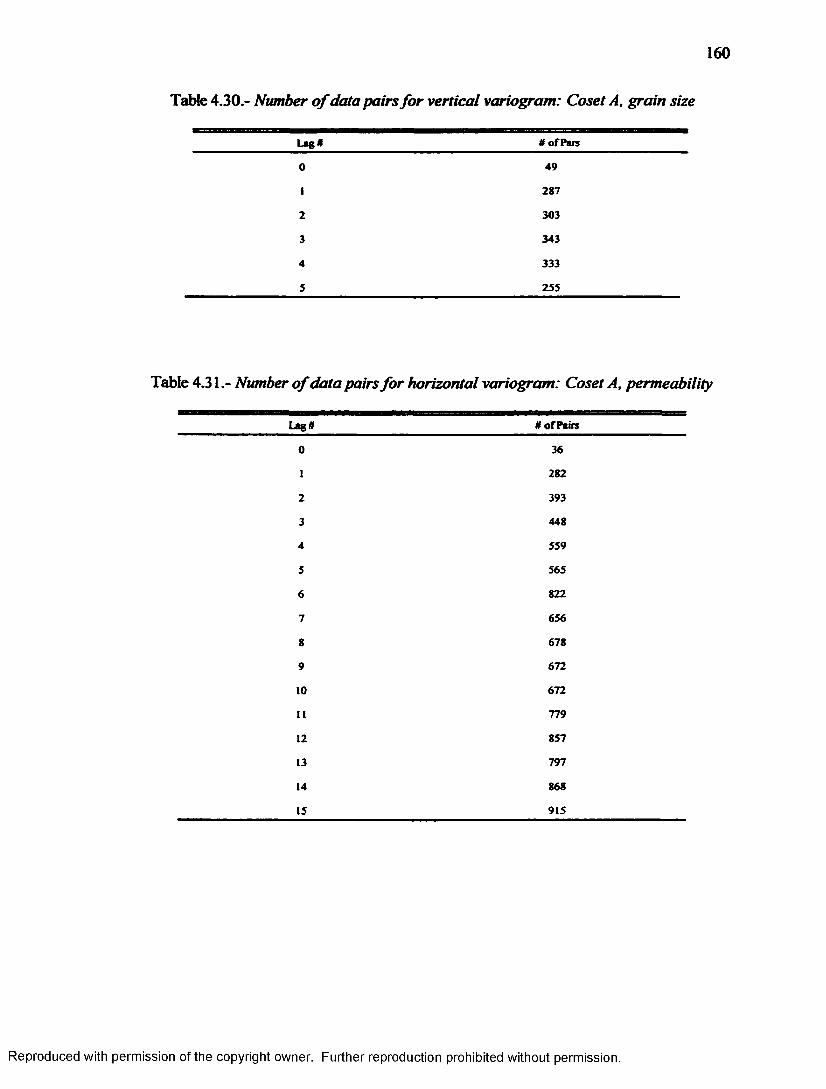
160

Table 4.30.- Number o f data pairs for vertical variogram: Coset A, grain size

Lag # * o f Pais

0 49

1 287

2 303

3 343

4 333

5 255

Table 4.31.- Number o f data pairs fo r horizontal variogram: Coset A, permeability

Lag # U o f Pairs

0 36

1 282

2 393

3 448

4 559

5 565

6 822

7 656

8 678

9 672

10 672

II 779

12 857

13 797

14 868

15 915


161

Table 4.32.- Number o f data pairs for vertical variogram: Coset A, permeability

L ag# # ofP aira

0 36

1 282

2 393

3 448

4 559

5 565

horizontally. This suggested geometry of grain size and permeability matches well with

the stratal geometry of the Oyster sediments. The lag spacing for this variogram was 0.1

meters, and the number of lags equaled 5 (Table 4.34).

Permeability Results. The permeability correlation structure for coset B is

similar to coset A in that a great amount of variability exists at small spatial scales. The

correlation length scale is 0.62 meters, which is smaller than the average set width for

coset B (Fig. 4.35). The variogram statistic Y (h) is quite large for all of the

permeability variograms compared to those o f grain size. Table 4.35 gives the

number of data pairs for each lag. Lag spacing is 0.2 meters, and the number of lags is

15. The vertical variogram of permeability for this coset was modeled using an

exponential fit, and shows a small correlation length scale of 0.25 meters. The number

of lags for this variogram is 11, with a lag spacing o f 0.1 meters (Fig. 4.36). Table 4.36

shows the number of data pairs for each lag.

Coset C

Grain Size Results. The horizontal variogram of grain size for coset C was

modeled using an exponential fit


r (IN)0.320.28

Direction 0

0.24

0.160.12

0.080.04

-►100 2 51 3 4 6 7 8 9

|h|

Fig. 4.33.- Horizontal variogram of grain size: Coset B.

7 (|h|) 0274-024 -

021 i

0.18 -

0.15 -

0.12 -

D irectio n 90

0.09

0.06

0.03

0 0.07 0.14 0.21 028 0.35 0,42 049 0.56 0u63|h|

Fig. 4.34- Vertical variogram o f grain size: Coset B.


D ire c tio n 0

1.2

1 m

0.8

0.6

0.4

0.2

00 0.5 1 1.5 2.5 32 3.5 4

IN

Fig. 4.35.- Horizontal variogram of permeability: Coset B.

/r(|h|) 2000'L

1800 -

D irection 90

160014001200

1000

800600400200

0 0.2 0.4 10.80.6M

Fig. 4.36.- Vertical variogram of permeability: Coset B.


164

The exponential variogram revealed a correlation length scale of 0.97 meters, with a sill

at 0.05. There are much less data points in this coset, therefore, an angular tolerance of

30 degrees was used. Also noticeable is the poorer modeling of the data in this coset

due to the lower number of data points (Fig. 4.37). The lag spacing is at 0.2 meters and

the number of lags is 9 (Table 4.37).

Table 4.33.- Number o f data pairs fo r horizontal variogram: Coset B, grain size

Lag# # o f Pairs

0 334

i 961

2 1232

3 1426

4 1SI6

S 1079

6 961

7 1387

8 1405

9 795

10 661

II 790

12 676

13 448

14 265

IS 600

16 398

17 264

18 4275

19 500

20 206

The vertical variogram of gram size yielded for coset C indicates a possible linear trend.

This is important because coset C contains a finning upwards sequence.


165

Table 4.34.- Number o f data pairs for vertical variogram: Coset B, grain sizeB E a B a B B E a n H B B B a H H H B B B M B a M a n B

Lag I # o f Pairs

0 76

1 164

2 133

3 (13

4 S7

5 82

Table 4.35.- Number o f data pairs for horizontal variogram: Coset Br permeability

Lag# # of Pairs

0 337

1 1384

2 1963

3 2168

4 2062

S 2266

6 2209

7 2270

S 2325

9 2222

10 2178

11 1908

12 I6S3

13 1S48

14 1458

IS 1330


166

Table 4.36.- Number o f data pairs for vertical variogram: Coset B. permeability

Lag * H of Pans

0 439

1 676

2 1223

3 1346

4 1211

5 1082

6 978

7 872

8 360

9 170

10 9

11 5

Table 4.37.- Number o f data pairs fo r horizontal variogram: Coset C. grain size

Lag U It of Pain

0 34

I 37

2 72

3 33

4 50

5 53

6 35

7 27

8 16

9 48


167

The lag spacing is 0.1 meters, with six lags (Fig. 4.38). Again, due to the small sample

size the variogram model is not as strong as it is for cosets A and B, and in this case a

model was not fit to the variogram. Table 4.38 gives the number of data pairs for this

variogram.

Permeability Results. The horizontal variogram for permeability of coset C was

constructed using a spherical model, which reveals a correlation length scale of 1.9

meters, with a lag spacing o f 0.1 meters and 12 lags. This is a larger correlation length

scale for permeability than either coset A or B (Fig. 4.39). One should notice that the

number of data pairs is significantly less than variograms of the other cosets (Table

4.39). The vertical variogram of permeability for this for this coset was also modeled

using a spherical fit. The spherical model for the vertical variogram for coset C revealed

a similar correlation length scale to that o f coset B (Fig. 4.40). The correlation length

scale is 0.23 meters, the lag spacing is 0.1 and the number of lags 5 (Table 4.40).

Table 4.38.- Number o f data pairs fo r vertical variogram: Coset C, grain size

Lag# # of Pans

0 19

1 56

2 37

3 28

4 40

5 19

6 7


168

Direction 00.081

0.072

0.063

0.054

0.045

0.036

0.027

0.018

0.009

►0.6 1.2 1.8 2.4 3.6 4.2 4.80 3

|h|Fig. 4.37.- Horizontal variogram of grain size: Co set C.

y (IN)i

0.081

0.072

0.063

0.054

0.045

0.036

0.027

0.018

0.009

0 • I

D ire c tio n 90

J ________ I_________I_________ I_________l_________ L

0.07 0.14 0.21 0.28 0.35 0.42 0.49 0.56IN

Fig. 4.38.- Vertical variogram o f grain size: Coset C.


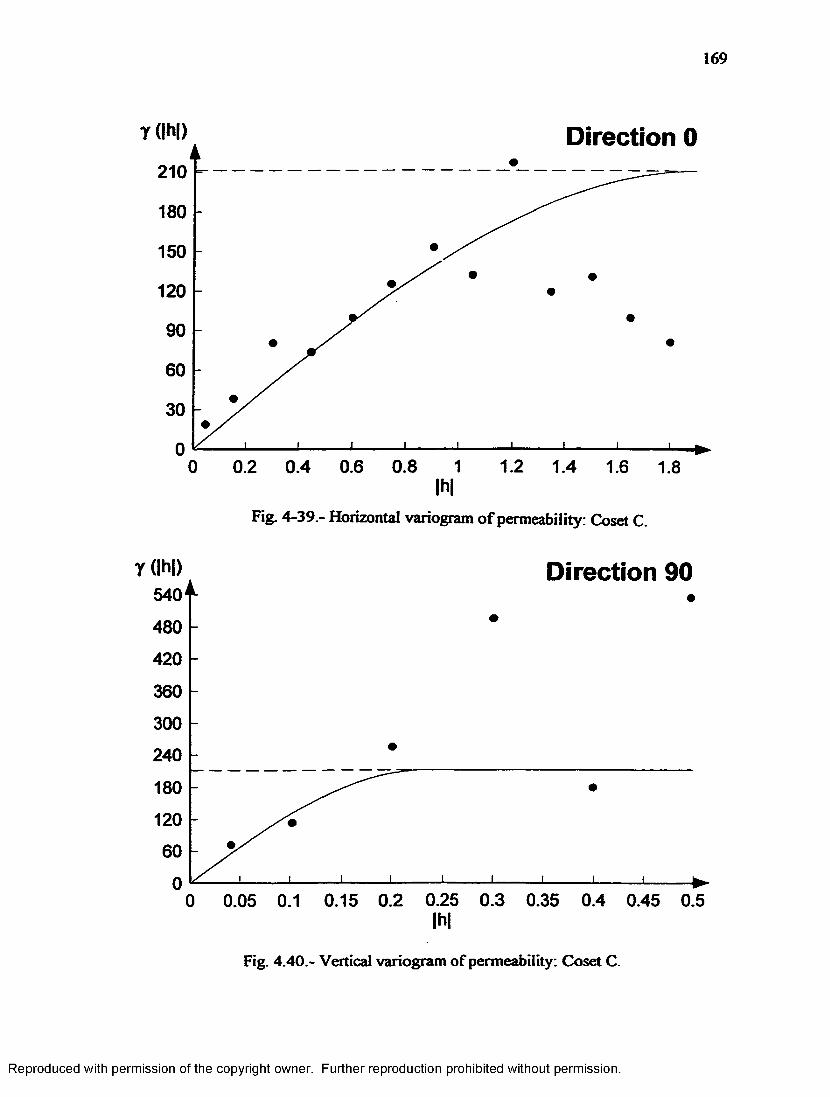
169

r (IN) Direction 0/ 1

210

180

150

120

0.2 0.4 0.6 0.8 1 1.2 1.4 1.6 1.80IN

Fig. 4-39.- Horizontal variogram o f permeability: Coset C

Direction 90

420360300240

180120

0 0.05 0.1 0.15 0.2 0.25 0.3 0.35 0.4 0.45 0.5IN

Fig. 4.40.- Vertical variogram of permeability: Co set C.


Table 4.39.- Number o f data pairs for horizontal variogram: Coset C, permeability

L ag# # ofPaws

0 22

i 215

2 2*5

3 259

4 283

S 281

6 330

7 305

8 314

9 360

10 375

11 460

12 396

Table 4.40.- Number o f data pairs fo r vertical variogram: Coset C, permeability

Lag # # o f Pairs

0 22

1 215

2 285

3 259

4 283

5 281


171

CHAPTER V

CONCLUSIONS

INTRODUCTION

The problem of the study is introduced in Chapter I, and an extensive review of

the subject is given. The hypothesis is formulated at the end of this chapter as welL It is

pointed out early in Chapter I that a fundamental concern of the stratigrapher is to

develop predictive models of stratigraphic organization. In sedimentology one of the

most significant problems that has yet to be resolved is the feet that there is a lack of

quantitative information regarding the relationship between geometry o f beds, thickness

of beds, grain size and sedimentary structures in sandy environments, especially shallow

marine deposits. Scientists have also realized the need to correlate quantitative

permeability data to sedimentary structures and scales o f stratigraphic organization. In

engineering this is called the physical heterogeneity o f a deposit The purpose of this

study is to investigate the scales of stratigraphic organization that control the variation of

grain size and permeability in shallow marine deposits. A model of stralal architecture is

constructed to relate scales of stratigraphic organization to these properties.

Stratigraphers typically construct one-dimensional facies models to understand scales of

stratigraphic organization. These facies models are used to define the large scale

heterogeneity of sedimentary deposits and have recently been used to construct regional

ground water models (Anderson 1989). Although fecies models are useful constructs

rooted in the physics o f sedimentation, this approach usually requires considerable

geologic interpolation, and is often unable to resolve the detailed spatial correlation of

primary and secondary textural properties. The construction o f fecies models does not


provide a means for representing uncertainties in the stratigraphic interpretation in more

than one dimension (Johnson et al. 1989; Bridge 1993). Smaller spatial scales are almost

entirety ignored in studies that relate reservoir and aquifer fluid properties to

stratigraphic organization. I suggest that this practice is inferior to the information that

can be obtained by constructing models o f stratal architecture to understand the

distribution of textural properties. A major goal of the study is to decide if stratigraphic

scales smaller than fecies are statistically significant to the distribution of grain size and

especially permeability. From the problem outlined above, the hypothesis found that

models of stratal architecture are more efficient predictors of grain size and permeability

than are fecies models in shallow marine sands.

In Chapter II, important questions related to the hypothesis were outlined, and

the methods used to test the hypothesis were described in detaiL One of the most

important questions investigated in the study is to what extent, are permeability and grain

size correlated to set boundaries? Several methods are used to test the hypothesis,

including mapping of stratal geometry, measuring stratal characteristics, and the

construction fecies distribution through measured sections. These techniques are used to

build the stratal architecture of the Oyster Site deposits. Bivariate plots are produced to

understand the depositional environment under which the Oyster Site deposits were

formed. AN OVA, Tukey-Kramer Means comparison tests and experimental variograms

are performed to test the statistical significance of mean grain size and permeability

variability over multiple scales of stratigraphic organization. Two major statistical

hypotheses are tested with the AN OVA tests. The statistical hypothesis formalized are:

(1) Null hypothesis- Mean grain size and permeability o f cosets are equal.


173

Alternative hypothesis- Mean grain size and permeability of cosets are not equaL

(2) Null hypothesis- Mean grain size and permeability of individual sets within a coset

are equaL

Alternative hypothesis- Mean grain size and permeability of individual sets within a coset

are not equaL

The Tukey-Kramer Means Comparison Tests determined which cosets and sets are

significantly different from one another with respect to grain size and permeability.

Horizontal and vertical experimental variograms for each coset are constructed in order

to decide the correlation length scales of grain size and permeability. The correlation

length scales are then compared with the scales of stratigraphic organization as a

separate technique from the ANOVAS in determining the scale over which the

distribution of grain size and permeability are most important.

Chapters III and IV contained all o f the results from the study. Chapter III

focused on the description of the architecture of the Oyster deposits, whereas Chapter

IV summarizes the results of the geo statistical analysis. In this chapter, I will relate the

results from Chapters III and IV to the hypothesis formulated, and explain the

significance o f the results.

SIGNIFICANCE OF THE OYSTER SITE ARCHITECTURAL RESULTS

Facies Architecture

The 1996 field campaign revealed three fecies, and one sub-fecies. These fecies

are a Cross-stratified sand fecies, a Horizontally stratified sand fecies, and Micro cross

stratified sand fecies. The Shelly gravelly sand fecies originally identified during the

1994 field initiative is actually a sub-fecies o f the cross-stratified sand fecies. Facies


were identified using a binomial nomenclature based on both grain size and stratal

architectural constructs (Fig. 3.9). Measured sections taken at every 2 meters

horizontally show that the upper section of the Butlers Bluff member in this exposure

consists of continuous Cross-stratified sand fecies and the less continuous Shelly gravelly

sub-fecies. The lower section of the Butlers Bluff member contains the Horizontally

stratified sand fecies and the Micro cross stratified sand fecies. When comparing the

fecies distribution diagrams (Fig. 3.3 through Fig. 3.6) to the stratal architecture maps

(Fig. 4.1, through Fig. 4.3), one can clearly see how much information is lost when

constructing one-dimensional fecies models. Neither the sections nor the standard

geological correlations between sections come close to predicting the actual geometry of

the deposits. Certainty, the geometric information gained from erecting a stratal

architectural model is fer superior to a one dimensional fecies model when attempting to

understand the depositional environment. Also, measurements of the stratal geometry

can be used as parameters that define “real” sedimentary structures in quantitative

models of aquifer and petroleum reservoirs.

Stratal Architecture

Chapter III showed that a modified McKee and Weir classification system can be

used to describe the stratal architecture o f the Oyster deposits. In this system, individual

lamina organizes to form lamina sets. Lamina sets organize to form genetically related

cosets, which organize further to form a composite set (Fig. 1.3). Cosets are analogous

to fecies volumes in the Oyster Site (Fig. 3.9). The significance of this is that by

constructing a model of stratal architecture in the Oyster Site, one can now relate the

distribution and variability o f grain size and permeability to scales of stratigraphic


175

organization and allow for the hypothesis to be tested.

Using the modified classification system o f McKee and Weir, four cosets were

recognized in the Oyster Site. Coset A is located in the uppermost section of the Oyster

Site and contains the Cross-stratified sand fecies and Shelly gravelly sand sub-fecies.

Beneath coset A, is coset B. This coset also contains the Cross-stratified sand fecies and

the Shelly-gravelly sand sub-fecies. Coset B is located in tier 2 of the Oyster Site, and

contains lamina thicknesses and widths that are generally larger than those in coset A.

Again, this is the type of information that is often overlooked when creating one

dimensional fecies models. The Shelly gravelly sand sub-fecies are the pebbly lag

deposits that are found at the base of the trough shaped cross strata sets. The pebbly lag

deposits are formed in scour pockets that contain the coarsest sediments. These scour

pockets formed in front of the linguoid dunes that migrated across the ancestral

Chesapeake Bay, and are created by leeside eddies (Smith 1972; Fig. 5.1).

Co set C, which is located in the lower part of the Oyster Site contains the Horizontally

stratified sand fecies. Sets are difficult to define in coset C, and are recognized by grain

size and color contrasts. Lamina and set widths are very continuous throughout this

co set, running wider than the exposure. Sets are also much thicker in Co set C than

Cosets A or B. Coset D which is located in the bottom most section of tier 3 of the

Oyster Site shows many similarities with cosets A and B. The main differences are that

lamina tend to dip at a 10-degree angle rather than 20 degrees, and that a wavy bedding

pattern is present. The wavy bedding is probably a diagenetic process, since the water

table is close. Another difference is that set widths are much larger in Coset D than they

are in A or B. In feet, set widths for this coset most closely resemble Co set C.


176


Fig.

5.1.-

The

form

ation

of

cross

strata

se

ts, n

otice

the

sc

our

form

ed

in fro

nt o

f the

m

igra

ting

dune

.

177

The ease at which the stratal architecture was constructed at this site shows that

this method is a generic classification system that enables the researcher to obtain the

maximum information from a sedimentary body. I contend that the construction of

simple generic models o f stratal architecture are superior to not only one-dimensional

fecies models, but to the architectural elements methods o f Miall and the bounding

surface numbering of Brookfield and Allen. The reason for this, is that the stratal

architectural model used in this study can be used anywhere without the implication of

the depositional environment. Miall’s architectural elements approach can only be used

in fluvial systems, and locks the investigator into narrow interpretations (Fig. 1.11). This

also holds true for Brookfield’s method, which is used mostly for aeolian deposits. Miall

clams that a similar approach can be developed for shallow marine deposits, but why

develop several models that can only be used in certain environments when a generic

system can be used without imposing a predetermined interpretation. The stratal

architectural approach can be applied uniformly to all environments unlike Miall’s or

Brookfield’s approach (Bridge 1993; Miall 1988; Brookfield 1977).

Vertical patterns of set thickness show a decrease upwards from the Lower

Butlers Bluff Member (Co set C) to the Upper Butlers Bluff Member (Co set A). A

vertical decrease in set thickness indicates that the water depth in which these sediments

were deposited was decreasing from Co set C to Co set A, and supports the theory that

the Butlers Bluff member represents the progradation of the Nassawadox Spit across an

ancestral Chesapeake Bay (Allen 1988; Fig. 3.26 through Fig. 3.30). Co set C and D are

the distal environment, whereas Co sets A and B represent the proximal environment

along a dispersal path in the ancestral Chesapeake Bay. Vertical patterns of grain size


178

within the architectural framework of the Oyster Site suggests a complex two-fold

nested trend. From the base of Coset C to the top of Coset A, (Lower Butlers Bluff to

Upper Butlers Bluff Member) a coarsening upward sequence o f mean grain size exists.

Coarsening upward sequences of grain size are also indicative o f a prograding shoreline

(Fig. 3.34). Within individual cross strata sets, a weak fining upward sequence of mean

grain size exists (Fig. 3.31 through Fig. 3.33). This pattern is the result of grain sorting

due the grains avalanching over ripple crests. As ripples or dunes migrate across the sea

floor, sediment accumulates on the lee side building up the crest. The ripple actually

migrates as sediment cascades down the stoss side of the bedform. During this process

the coarser grains settle fester than the finer grains, therefore, the finer grains are

deposited higher up in the avalanching lamina. Between successive avalanching

episodes, grains settle out of suspension on the stoss side of the ripple. This entire

process creates the alternating coarse and fine lamina pattern exhibited in the Oyster Pit

sediments (Jopling 1963; Allen 1984).

Progressive Sorting on the Nassawadox Shoreface

General. To understand the architectural results of the Oyster She fully, h is

necessary to understand the processes in which fecies or cosets were formed. Facies are

typically defined by horizontal grain size gradients in the order o f meters to kilometers,

and by vertical grain size variations on the scale o f millimeters to centimeters. Several

authors describe “cook-book” rules for applying fecies models and erecting fecies

schemes (Reading 1978; Walker 1989; Miall 1990). Articles addressing fecies and fecies

models rarely show any insight as to the dynamics responsible for fecies differentiation.

Swift et aL (1991a) has pointed out that in shallow marine settings, fecies are produced


179

during sediment dispersal by the combined processes of progressive sorting and stratal

condensation. During the progressive sorting process, facies become differentiated as

sediment moves down the dispersal pathway in response to episodic transport events

such as storms. Russel (1939) recognized that in such settings the competence o f the

transporting agent would decrease downstream as a result of the fluid power gradient.

As a consequence of the decreasing competence, the coarsest particles are selectively

deposited in the proximal environments. The coarsest particles entrained during episodic

events are isolated in the sole o f the bed formed as the current wanes. If the next event

is less intense, then only the upper portion o f the bed will be re-suspended or re

entrained. Therefore, over time, finer sediments are preferentially bypassed to

downstream environments, and grain size will vary from proximal to distal locations

along the dispersal pathway. Beds or lamina in the proximal environments retain the

coarsest particles due to the energetic environment, whereas, finer grained beds and

lamina are deposited in distal environments (Fig. 5.2). This process leads to stratal

condensation (Swift et a l 1991a). In the proximal environments where fluid power is

high, each resuspension event tends to strip off the fine caps of the previous event.

Therefore, only the truncated bases of the beds deposited by the rare intense events are

preserved. This leads to a coarse stratally condensed deposit in which thick lam ina or

beds are preserved. In proximal environments cross-stratified deposits are common due

to the feet that most sediment in traveling as bedload. As the fluid power decreases

down the dispersal path, bed successions become less condensed as the finer caps are

preserved from each event. In the far distal environment sediment source becomes a

factor. The coarse sands have been left behind, and only the finest sand, silt and clay is


180

ProximalStation

T1

T2

DistalStation

\

M

Fig. 5.2.- The progressive sorting mechanism acting through time steps T1-T3 (after Swift etal. 1991a).


181

left. This causes another condensed section in the far distal environment because

individual beds are difficult to differentiate. Lamina or beds in this environment are

typically either laminated or bioturbated (Swift et aL 1991a). Swift et aL (1991b)

illustrates the textures and structures that are the result of the progressive sorting

process in shallow marine settings (Fig. 5.3).

We see can the same processes working on the Nassawadox shelf. Sand moved

along the oceanward side of the spit in a storm driven pulses in a narrow (100m wide)

zone of shoaling and breaking waves. During peak flow events, rip currents expelled

fluid and sand from the surf zone, and sand rained out on the shorefece. Washed residue

retained by the surf zone was medium to coarse, pebbly sand, while the winnowed

fraction deposited on the shoreface consisted of fine sand (Fig. 5.4). This is an example

of progressive sorting, and has led to the fecies differentiation and the stratal architecture

of the Oyster Site.

Progressive sorting has induced further effects. Medium and coarse sand travels

as bed load, and bed load transport is accomplished entirely by migrating bedforms

(ripples, dunes). These migrating bedforms deposit sediment into a characteristic cross

stratification patten (Collison and Thompson 1982; Fig. 5.1), therefore the medium sand

fecies is a cross stratified fecies (Coset A and B). The fine sand rains out o f suspension

in the distal environment to form horizontally layered strata sets as the current wanes.

Therefore, the fine sand fecies is a horizontally stratified fecies (Coset C). In our case,

small bodies of the Cross Stratified, medium Sand fecies, and the Shelly-gravelly coarse

Sand fecies are intimately admixed. In feet, the Shelly-gravelly sand facies are analagous

to Swift’s lag strata from the Mesaverde Sandstone (see Fig. 5.3).


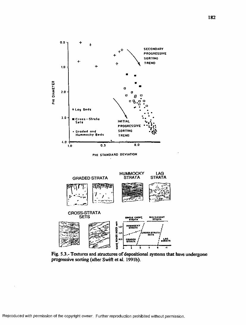
PHI

OIAM

ETER

182

0.0 -i

SECONOARYPROGRESSIVE

SORTINGTREND

2.0 -

+ L ag B e d s

■ C r o s s —S t r a t a S e t s INITIAL

PROGRESSIVE

SORTINGTREND

G r a d e d a n d H u m m o c k y B e d s

(.00 .00.51.0

PHI STANDARD OEVIATION

GRADED STRATA

. / _•* ve-'O*.-

H U M M O C K YSTRATA

L A G

STRATA

CROSS-STRATASETS SINGLE EVENT,

STRATA

7

^*

HUMMOCKY STRATA ,

MULTLEVENTSTRATA

-*'7 /CROSS-STRATA/I SETS t 9 I

GRAOEO / STRATA l

i LAG t STRATA

Fig. S.3.- Textures and structures of depositional systems that have undergone progressive sorting (after Swift et al. 1991b).


Shelly Gravelly Facies A

Cross-StratifiedFacies

Coarse

AtSdbpopulallone SafcaHon Deposit (Sand)BisubpopdaUon:SuspersionDepost(sand)

CSUbpopdaHon; Traction Depost (Gravel)

Horizontally Stratified Facies

B

Fig. 5.4.- Progressive sorting on the Nassawadox shoreface.

184

The progressive sorting process is distinctly illustrated in the bivariate plots constructed

of textual properties. A significant linear relationship exists between mean grain size and

sorting, which shows the segregation o f the Horizontally stratified sand facies from the

other three (Fig. 4.4). Notice how closely Fig. 4.4 resembles Fig. 5.3. Bivariate plots of

mean grain size vs. % gravel, sorting vs. % gravel, and even grain size vs. permeability is

indicative of the progressive sorting process at work on the Nassawadox shoreface (Fig.

4.6 and Fig. 4.9). Mean grain size shows a weak but significant linear relationship to

permeability. This indicates that other factors control permeability and grain size.

Interestingly, sorting shows almost no relationship to permeability. Grain packing most

likely has the most significant effect permeability. However, this is beyond the scope of

the research. One of the most significant results from the bivariate plots is the

relationship between set thickness and mean grain size.

Mean Grain Size vs. Set Thickness. The relationship between set thickness and

grain size was investigated at the Oyster Site. Previous work by Schwarzacher (1953)

suggests that a positive linear relationship between bed thickness and median grain size

exists. The R2 of this relationship is 0.34. This demonstrates a weak but significant

relationship between the two variables. In a paper by Scheidegger and Potter (1967), the

same data are used and a log-log plot is created. The coefficient of correlation was not

reported, but it is obviously the same as the previous study. The authors of this study

claim that larger sand wave heights are associated with greater turbulence, therefore

allowing coarser grains to be transported. On the surface this idea may sound good, but

some problems exist. The idea that as ripple or dune height increases, the turbulence

increases causing a more competent flow suggests that dune height directly affects the


185

grain size o f a deposit. If turbulence is so great, then a significant amount of scouring

must be occurring, so how can thick deposits be formed? Since grain size directly affects

the transporting mode of a sediment, does Scheidegger and Potter’s statement realty

make sense? It seems more likely that grain size would affect dune height, not the other

way around.

The relationship between set thickness and mean grain size was studied further at

the Oyster Site. Both cross-bedded deposits and horizontally stratified deposits were

used in the study. Figure 4.10 shows that a non linear relationship exists between these

two variables. In fact, the relationship is parabolic and the R2 is considerably higher

(0.5) then that of Schwarzacher. The parabolic relationship found between grain size

and set thickness is significant at the 99% confidence level One could probably fit the

same parabolic curve to Schwarzacher’s data and produce similar results as was found at

the Oyster Site. The relationship also shows that a minimum occurs at 1.5 phi or

0.35mm. The parabolic relationship recognized between mean grain size and set

thickness has a familiar shape to sedimentologists. The curve is sim ilar to the well-

known HjOlstrom curve that relates current velocity necessary for erosion and grain size

(Fig.5.5). The HjOlstrom curve illustrates that the coarsest and finest grain sizes are the

most difficult to erode. The minimum point on this diagram occurs at 0.35mm or 1.5

phi. Sand grains whose size is between 0.1mm and 0.2mm are the most mobile, and

usually only require a velocity of about 0.3 m/s to be transported (Seibold and Berger

1982). In comparison, the relationship between set thickness and mean grain size shows

that the minimum occurs at about the same grain size. This suggests that the coarsest

and finest sands produce the thickest deposits.


Vel

ocity

, in

cent

imet

er*

per

seco

nd

186

2000

EROSION

SITION

Pebble fGryel). -^Cobfa^fBoyfcte^- C laye e a r n « coeoo o o pop o o ooo o o 000

o 00- n e eiaio o o 000 o o 000" ^ « <DOOO O O O O O

e c o o o o

r cv e «o" - . _O o o O O p O O o p o 0 9 9 9 qpo o o 00 oO o o 00 .........................................Gram sue. in millimeters

Fig. 5.5.- Hjulstrom curve, relating grain size to velocity (after Seiboki and Berger 1982).


187

However, unlike the HjQlstrom, the relationship found between set thickness and mean

grain size is not caused by electrostatic forces. Instead, the parabolic relationship found

between set thickness and mean grain size is the result o f the coupled processes of

progressive sorting and stratal condensation. This makes more sense than a linear

relationship because o f the Hjtilstrom relationship.

In the proximal environment of a dispersal system, the coarsest sediment moves

as bedload forming ripples and dunes as well as coarse lag deposits. Therefore thick

deposits are preserved, since the coarse particles are difficult to erode. The finer

sediments are carried down the dispersal system, following the fluid power gradient.

Since grain sizes between 0.1 and 0.2 mm are the easiest to erode, only thin deposits are

preserved with these grain sizes. At the distal end of the dispersal system, the finest

sands are deposited as the current wanes. Once these grains are deposited they are much

more difficult to suspend then they were to carry. Thus, thick deposits are also

preserved. This suggests that the relationship between mean grain size and set thickness

is the evolutionary consequence o f the progressive sorting and stratal condensation

processes. In feet, the process o f progressive sorting necessitates the parabolic

relationship found between grain size and set thickness, not a linear one.

SIGNIFICANCE OF ANOVA RESULTS

Results of the ANOVA test and the Tukey-Kramer Mean Comparison test

indicate that Cosets are significantly different from one another with respect to grain size

and permeability (Fig. 4.13 and Fig. 4.19). This comes as no surprise because Co sets are

analogous to fecies volumes we should expect to see significant differences between

fecies. More importantly, the ANOVA results clearly show that individual sets can be


distinguished from one another with respect to grain size and permeability as well (Fig.

4.20 through Fig. 4.27). In fact, the mean comparisons test show that more than one set

is significantly different from one another within each Co set, indicating that set grain size

and permeability is an important stratigraphic scale and mappable. The ANOVA tests

prove that grain size and permeability variability is significant over multiple scales of

stratigraphic organization. Also, another important result from the means comparisons

tests are the recognizable patterns of sets in a coset that are significantly different. Those

sets that are significantly different from one another with respect grain size are usually

significantly different with respect to permeability. Careful examination of the means

comparisons results for each coset reveals that in general, sets occurring at the top of a

particular coset are significantly different from sets occurring in the middle of the coset

but not to each other. Also, sets occurring at the base o f a coset are significantly

different from those at the middle, but not to each other. Finally, sets at the base may or

may not be significantly different from those at the tops o f a coset (Table 4.14; Fig. 4.1).

This pattern occurs in all four cosets, and suggests that yet another scale of stratigraphic

organization is operating here that is also important to grain size and permeability

variations. For historical purposes I will can this the bed scale. Therefore, in the Oyster

Site of the Butlers Bhiff Member the stratal architecture contains lamina that build

lamina sets. Lamina sets build beds, and beds build cosets. One should recognize

immediately that the stratigraphic organization described above actually more closely

resembles Campbell’s classification system (Table 1.7). Therefore, the mean

comparisons test proved that not only are individual sets significant with respect to grain

size and permeability distributions, but that the preferred stratal architectural


189

c lassification system may be Campbell's instead of McKee and Weir.

SIGNIFICANCE OF VARIOGRAM RESULTS

Variograms are constructed as an independent test of the scale of stratigraphic

organization at which grain size and permeability demonstrate the most variability.

Results from the variograms indicate that for both grain size and permeability the

correlation length scales were always smaller than set widths or thicknesses. This held

true for each coset tested. The horizontal correlation length scale for grain size was

typically around 0.6 meters except for Coset B. Coset B has a correlation length scale

for grain size of 2.0 meters (Fig. 4.33). Average set widths for Co sets A and B is 5

meters. Vertical correlation length scales for grain size and permeability were always

less than set thicknesses. The variogram results indicate that grain size and permeability

exhibit a high degree of spatial variability. Since correlation length scales were always

less than set widths and thicknesses, one can infer that the lamina scale is also significant

with respect to the spatial variability of grain size and permeability. Actually, the lamina

scale is probably the most significant stratigraphic scale for understanding the

distribution of grain size and permeability because o f the small correlation length scales.

GENERAL CONCLUSIONS

The ANOVA test, means comparisons test and the variograms all prove that

multiple levels of stratigraphic organization are statistically significant with respect to the

spatial variability of grain size and permeability, and the one-dimensional facies models

are clearly unable to resolve these important stratigraphic scales. This study clearly

shows that models o f stratal architecture are more efficient predictors of grain size and

permeability than are fecies models in shallow marine deposits. Traditional methods


190

such as coring and log studies can only develop lithofacies models that can not duplicate

the complexities of the geologic framework. The stratal architectural model is more than

just a nomenclature for stratigraphic organization, for it actually defines the shape and

scale of sedimentary deposits at multiple scales. Knowledge of the shape and scale of

the sedimentary structures over several stratigraphic scales will aid in the prediction local

deviations from regional groundwater and petrophysical models because the geological

complexity can be built into the models. The study also suggests that a simple generic

model of stratal architecture is a better approach to the understanding of sedimentary

deposits and their associated textural properties than environment specific complex

architectural element or bounding surface numbering approaches, because it does not

require one to approach the outcrop with a predefined genetic interpretation for each

bounding surface. Bivariate plots of textural properties indicate that progressive sorting

shaped the stratal architecture of the Oyster Site in the Butlers Bluff Member. A

parabolic relationship was discovered to exist between mean grain size and set thickness,

and is thought to be the evolutionary consequence of the progressive sorting process.

FUTURE RESEARCH

Suggestions for future research on this subject include a detailed investigation of

grain size and permeability on the lamina scale by using small box cores. Also, the third

dimension (set length) should be fully measured and mapped in order to fully describe the

three-dimensional architecture of shallow marine deposits. Unfortunately this was not

possible during this study. I also suggest measuring the spatial variation of permeability

in two directions (width and length) to determine how much the internal geometry of

sedimentary deposits control the permeability structure. Finally, the relationship between


191

set thickness and mean grain size should be investigated to see if it really is a universal

relationship to all sedimentary environments.


192

REFERENCES

Allen , J.R.L., 1963, The Classification o f Cross-stratified Units,With Notes on Their Origin: Sedimentology, v. 2, p. 93-114.

Allen , J.R.L., 1965, On Bedforms and Paleocurrents: Sedimentology, v.6, p. 153- 190.

Allen , J.R.L., 1968, The Nature and Origin of Bed-Form Heirarchies:Sedimentology, v.10, p. 161-182.

A llen , J.R.L., 1973, Features of Cross-Stratified Units Due to Random and other Changes in Bedforms: Sedimentology, v. 30, p. 189-202.

ALLEN, J.R.L., 1984, Sedimentary Structures. Their Character and Physical Basis, in E)evelopments of Sedimentology, v. 1 and 2, n. 30, p. 663.

Allen , J.R .L ., 1988, Sandwaves: A Model O f Origin and Internal Structure: Sedimentary Geology, v. 26, p. 281-328.

Allen , P. A., An d Allen , J. R. L., 1990, Basin Analysis, Principles and Practice, London, Blackwell Scientific Publishing.

An d er so n , M. P., 1989, Hydrogeologic Facies Models to Delineate Large-Scale Spatial Trends in Glaciofluvial Sediments: Geological Society of America Bulletin, v.101, p. 501-511.

BlERKENS, M . F., AND W e e r t s , H.J.T., 1994, Block Hydraulic Conductivity of Cross- Bedded Fluvial Sediments: Water Resources Research, v. 30, n. 10, p. 2665- 2678.

B oyd , R., Suter, J., Penlan d , S., 1989, Relation of Sequence Stratigraphy to Modem Sedimentary Environments: Geology, v. 16, p. 925-929.

BRIDGE, J.S., 1976, Origin of Horizontal Lamination Under Turbulent Boundary Layers: Sedimentary Geology, v. 20, p. 1-16.

B rid g e , J.S., 1993, Description and Interpretation of Fluvial Deposits: A Critical Perspective: Sedimentology, v. 4 0 , p. 801-810.

BROOKFIELD, M .E ., 1977, The Origin of Bounding Surfaces in Ancient Aeolian Sandstones: Sedimentology, v. 24, p. 303-332.

C a m bell , C .V ., 1967, Lamina, Lamina Set, Bed, Bedset: Sedimentology v. 8, p. 7- 26.

C arr , J. 1995. Numerical Analysis for the Geological Sciences: New Jersey, Prentice Hall, p. 592.

C handler, M., Kocurek , G., Go g g in , D., a n d Lake, L., 1989, Effects ofStratigraphic Heterogeneity on Permeability in Eolian Sandstone Sequence, Page Sandstone, Northern, Arizona: American Association of Petroleum Geologists Bulletin, v. 73, n. 5, p. 658-668.

C o ch ra n , W.G., 1947, Some Consequences When the Assumptions for the Analysis of Variance are not Satisfied: Biometrics, v. 3, p. 22-38.

C ollision , J.D., and Th o m pso n , D.B., 1982, Sedimentary Structures: in London, Allen and Unwin, eds., 94 p.

C olquhoun ,D ., Joh nson , G.H, Peebles, P. C., Huddleston , P. a n d Scott, T., 1991, Quaternary Geology of the Atlantic Coastal Plain, :The Geological Society of America Bulletin, in The Geology of North America Quaternary


193

Nonglacial Geology: Conterminous United States, v. K-2.Cr o m a n , D. S ., 1972, Skewness and Kurtosis in Polymodal Sediments from the Irish

Sea: Journal of Sedimentary Petrology, v. 42, p. 102-106.Cu sh m a n , J.H. 1990, Dynamics of Fluids in Hierarchical Porous Media: San Diego,

Academic Press, 505 p.D a v i s , J.C., 1 9 8 6 , Statistics and Data Analysis in Geology, Second Edition: John

Wiley and Sons, New York, 6 4 6 p .D a v is , J.M., Lo h m a n ,R ., P h illips, F., W il so n , J., A n d Lo v e , D., 1993,

Architecture of the Sierra Ladrones Formation, Central New Mexico: Depositional Controls on the Permeability Correlation Structure: Geological Society of America Bulletin, v. 105, p.998-1007.

D a v is , J.M , W il so n , J.L., a n d Ph illips, F.M, 1994, A Portable Air -Minipermiameter for Rapid in-situ Field Measurements: Ground Water, v.32, n. 2, p. 258-266.

D a v is , J.M., W il so n , J.L., Ph illips, F.M., Goixowrrz, M B., 1997, Relationship Between Fluvial Bounding Surfaces and the Permeability Correlation Structure: Water Resources Research, v.33, n.8, p. 1843-1854.

Do y le, J.D. and Sw eet , ML., 1995, Three-Dimensional Distribution of Lithofacies, Bounding Surfaces, Porosity, and Permeability in a Fluvial Sandstone - Gypsy Sandstone of Northern Oklahoma: American Association of Petroleum Geologists, v. 79, n. 1, p.70-96.

Duncan, D. B., 1955, Multiple Range and Multiple F Tests: Biometrics, v. 11, p. 1- 42.

Fish er , W. L. An d M cG o w e n , 1967, Depositional Systems in the Wilcox Group of Texas and their Relationship to the Occurance of Oil and Gas: Gulf Coast Association Geological Society Transactions, v. 17, p. 105-125.

Fl em m in g , B .W . a n d B a rh o lo m A, editors, 1995, Tidal Signatures in Modem and Ancient Sediments,

Fo lk , R.L., a n d W a r d , W.C., 1957, Brazos River Bar. A Study in the Significance of Grain Size Parameters: Journal of Sedimentary Petrology, v. 27, n. 1, p. 3- 26.

Fo lk , R.L., 1980, Petrology o f Sedimentary Rocks: Austin, Texas, Hemphill Publishing Company, 154 p.

Fr e y b e r g , D.L., 1986, A Natural Gradient Experiment on Solute Transport in a Sand Aquifer 2. Spatial Moments and die Advection and Dispersion of Nonreactive Solutes: Water Resources Research, v. 22, n. 13, p. 2031-2046.

Friedm an , G. M ., 1967, Dynamic Processes and Statistical Parameters Compared for Size Frequency Distribution of Beach and River Sands: Journal of Sedimentary Petrology, v. 37, p. 327-354.

Garabedian , S.P., Lebla n c , D.R., Gelhar, L.W., and Celia , M.A., 1991, Large- Scale Natural Gradient Tracer Test in Sand and Gravel, 2, Analysis of Spatial Moments for a Nonreactive Tracer Water Resources Research, v. 27, n. 5, p. 911-924.

Gogchn, D.J, T h r a sh er , J.R. AND Lake, L ., 1988, A Theoretical and Experimental Analysis of Minipermeameter Response Including Gas Slipage and High


194

Velocity Flow Effects: In Situ. v. 12, p. 79-116.Harms, J.C. and Fahnestock , R.K., 1965, Stratification, Bedforms and Flow

Phenomena (with an example from the Rio Grande), in, Primary Sedimentary Structures and their Hydrodynamic Interpretation, SEPM Special Publication, n. 12, p. 84-115.

Hann , C.T., 1977, Statistical Methods in Hydrology: The Iowa State University Press, 387 p.

Hearn,C.L., Eban ks,W .J., Tyer,S ., Ranganthan ,V ., 1984, Geological Factors Influencing Reservoir Performance of the Hartzog Draw Field, Wyoming: Journal of Petroleum Technology, v. 34, p. 1335-1344.

Hess, BC.M. Wolf, S.H., Celia , M.A., 1992, Large-Scale Natural Gradient Tracer Test in Sand and Gravel, Cape Cod, MA, 3. Hydraulic Conductivity Variability and Calculated Macrodispersivities: Water Resource Research, v. 28, n. 8, p. 2011-2027.

HsO, K., 1989, Physical Principles of Sedimentoloy, A Readable Textbook for Beginners and Experts: New York, NY, Springer-Verlag.

Isaaks, E. H , and Srvastava , R. M., 1989, Applied Geostatistics: New York, Oxford University Press.

Johnson, G.H., Ward , W. Peebles, P.C., Stratigraphy and Paleontology of Pliocence and Pleistocence Deposits of Southeastern, Virginia^

Johnson, N. and Dreiss, S., 1989, Hydrostratigraphic Interpretation UsingIndicator Geostatistics: Water Resources Research, v. 5, n. 12, p.2501-2510.

J o pu n g , A.V., 1963, Hydraulic Studies on the Origin of Bedding: Sedimentology, v.2, p. 115-121.

Jo pu n g , A V., 1965, Laboratory Study of the Distribution of Grain Sizes in Cross- Bedded Deposits, in Middleton,G.V., ed., Primary Sedimentary Structures and their Hydrodynamic Interpretation, Publication n. 12.

Jopun g , A V., Allen , J. R. L., and W alker , R.W., 1968, Morphology and Origin of Ripple-Drift Cross-Lamination, with Examples from the Pleistocene of Massachusetts: Journal of Sedimentary Petrology, v. 38, p. 971-978.

Koltorm a n , C.E. AND GORUCK, S. M , 1996, Heterogeneity in SedimentaryDeposits: A Review of Structure-Imitating, Process-Imitating, and Descriptive Approaches: Water Resources Research, v. 32, p. 2617-2658.

Kramer, C. Y., 1956, Extension of Multiple Range Tests to Group Means with Unequal Numbers of Replications: Biometrics, v. 12, p. 307 to 310.

Lake, L a n d C a rro l , H.B., 1986, Reservoir Characterization: New York,Academic Press.

Lake, L., Carrol, HB. and Wesson,T.C., 1991, Reservoir Characterization II: New York, Academic Press.

Liu, K., Boult , P., P ainter, S., and Paterson , L., 1996, Outcrop Analog For Sandy Braided Stream Reservoirs: Permeability Patterns in the Triassic Hawkesbury Sandstone, Sydney Basin, Australia: American Association of Petroleum Geologists Bulletin, v. 80, n.12, p. 1850-1866.

M arzo , M , N u m a n , W ., Pu ig d efa b r eg a s , C., 1979, Architecture o f the Castissent Fluvial Sheet Sandstones, Eocene, South Pyrenees, Spain: Sedimentology,


195

v.35, p.719-738.M cBrid e , E.F., Sheperd, R.G. a n d Craw ley JLA., 1975, Origiii of Parallel, Near-

Horizontal Laminae By Migration of Bed Forms in a Small Flume: Journal of Sedimentary Petrology, v. 45, n. 1, p. 132-139.

M c C a m m o n , R. B., 1976, A Practical Guide to the Construction of Bivariate Scatter Diagrams: Journal of Sedimentary Petrology, v. 51, p. 616-624.

M c k e e , E d w in D. An d W e ir , G., 1953, Terminology for Stratification and Cross- Stratification in Sedimentary Rocks: Bulletin of the Geological Society of America, v. 64, p. 381-390.

M cLlNG, T. L. an d HIGGS, B., 1996, Field Characterization and Sampling Plan for Outcrop Studies at the Oyster, Virginia Bacterial Transport She Borrow Pit, Unpublished Report to the Department of Energy, Idaho National Engineering Labs, Idaho Falls, Idaho.

Mia ll , A.D., 1988, Facies Architecture in Clastic Sedimentary Basins: in Kleinspehn, K.L., and Paola, C.,eds., New Perspectives in Basin Analysis, New York, Springer-Verlag, p. 67-82.

M ia l l , A. D., 1985, Archhectural-Element Analysis; A new method of faciesanalysis applied to fluvial deposits: Earth Science Reviews, v. 22, p. 261-308.

M lA L L , A. D., 1990, Principles of Sedimentary Basin Analysis, Second Edition: New York, Springer-Verlag.

M id d l e t o n , G.V., 1965, Primary Sedimentary Structures and their hydrodynamic Interpretation: in Society of Economic Paleotologists and Mineralogists, n_12.

M id d l e t o n , G.V., 1977, Sedimentary Processes: Itydraulic Interpretation of Primary Sedimentary Structures: m Society of Economic Paleontologists and Mineralogists, Reprint Series n. 3.

M lX O N , R.B., 1985, Stratigraphic and Geomorphic Framework of the Uppermost Cenozoic Deposits in the Southern Delmarva Peninsula, Virginia and Maryland: United States Geological Proof Paper 1067-G, 53 p.

M u l l er , A .C ., Parsons, B .S ., Sw ift , D J .P ., 1996, C om parison betw eenPetrographic, Photo mosaic, and Core “Facies”, Oyster Site: Preliminary Report to the Bacterial Transport Program, Department of Energy. Contribution #13, of the Sediment Dynamics Group, Old Dominion University, Norfolk, VA.

NEIDORODa,A.W. and SWIFTJ3.J.P, 1991, Shoreface Processes, Chapter 13, in Herbie,J.B. ed., Handbook of Coastal and Ocean Engineering, Volume 2: Houston, TX, Gulf Publishing Company.

Olo riz ,F .,Caracuel,J.E., and Ru iz-Hera s,J. 1995, Numerical analysis of sedimentary components: A key for interpretation of macroscopic and microscopic features in Ammonitico Rosso fecies (Uppermost Jurassic- Lowermost Cretaceous): Journal of Sedimentary Research, v. A65, n.1, p. 234-243.

O w e n s , J.P. a n d Den n y , C.S., 1979, Upper Cenozoic Deposits of the Central Delmarva Pennisula, Maryland and Delaware: United States Geological Survey Professional Paper 1067-A.


196

P a n d a , M.N. and La k e , L.W., 1995, A Physical Model Of Cementation and its Effects on Single-Phase Permeability: American Association of Petroleum Geologists Bulletin, v. 79, n. 3, p. 431-443.

Pannatier ,Y ., 1996, Variowin, Software for Spacial Data Analysis in 2D: New York, NY, Springer.

P a r so n s , B.S., 1998, Sedimentary Facies and Systems, Stratigraphy in a Barrier Spit Complex: Unpublished Doctoral Dissertation, Old Dominion University, Norfolk, Va.

P a sseg a , R., 1964, Grain Size Representation by CM Patterns as a Geological Tool: Journal of Sedimentary Petrology, v. 34, p. 830-847.

P a sseg a , R., 1977, Significance of CM Diagrams of Sediments Deposited by Suspension: Sedimentology, v. 24, p. 723-733.

Pe t t u o h n , F. J.; Po tter , P. E.; a n d Siev er , R., 1972, Sand and Sandstone: New York, Springer-Verlag.

R a m se y ,K .W ., 1992, Coastal Response to Late Pliocene Climate Change: Middle Atlantic Coastal Plain, Virginia and Delaware, in Quaternary Coasts o f the United States: Marine and Lacustrine Systems: SEPM Special Publication 48, p. 121-127.

R e a d in g , H ., 1982, Sedimentary Environments and Facies, New York, Elsevier.SAS INSTITUTE, Inc., 1995, JMP® Statistics and Graphics Guide, Version 3. lO:

Cary, NC, USA, SAS Institute Inc.Saville , D.J., 1990, Multiple Comparison Procedures: The Practical Solution: The

American Statistician, v. 44, p. 174-180.Scheibe ,T .D ., 1993, Characterization of the Spatial Structure of Natural Porous

Media and its Impacts on Subsurface Flow and Transport: Ph.D. Dissertation, Stanford University, California.

Sc h e id e g g er ,A .E. a n d Po tter^ .E ., 1967 Bed Thickness and Grain size: Cross- Bedding: Sedimentology, v. 8, p. 39-44.

SCHIEDLER, G. L., LUDWICK, J., OERTEL, G .F., AND FlNKELSTEIN ,K ., 1984,Quaternary Stratigraphic Evolution of the Southern Delmarva Peninsula Coastal Zone, Cape Charles Virginia: Geological Society of America Bulletin, v.95, p.489-502.

SCHWARZACHER,W., 1953, Cross-Bedding and Grain Size in the Lower Cretaceous Sands of East Anglia: Anglia Geol. Mag., v. 90, p. 322-330.

S e lf , G.A. and S c o t t , R.W., 1993, Can Lithology Be Predicted from StratalArchitecture? An Emperical Approach to the Sequence Stratigraphy of the Plio-Pleistocence, Gulf of Mexico: 25th Annual Offshore Technology Conference, Houston, TX, OTC7124.

Se ib o l d , E . An d Be r g er , W .H ., 1982: The Sea Floor, A n Introduction to Marine Geology, New York, Springer-Verlag.

S im p so n , EX. a n d Er ik sso n JfC.A., Depositional Facies and Controls onParasequence Development in Siliclasitc Tidal Deposits from the Lower Proterozoic, Upper Mount Guide Quartzite, Mount Isa Inleir, Australia: in. Clastic Tidal Sedimentology, Memoir 16, p.371-387.

S m ith , L., 1981, Spatial Variability of Flow Parameters in a Stratified Sand:


197

Mathematical Geology, v. 13, n.1., p. 1-21.SMITH, N. D ., 1972, Some Sedimentoligical Aspects of Planar Cross-Strata in a Sandy

River. Journal of Sedimentary Petrology, v. 42, p. 624-631.SORBY, H.C., 1859, On the Structures Produced by the Currents Present During the

Deposition of Stratified Rocks: Geologist, v. 2., p. 137-147.Sw ift , D. J. P., and Thorne, J. A., 1991a, Sedimentation on Continental Margins,

Part I: A General Model for shelf Sedimentation, in: Swift, D. J. P., Tillman, R. W., Oertel, G. F., and Thome, J. A., eds., Shelf Sand and Sandstone Bodies: Geometry, Facies and Sequence Stratigraphy: International Association of Sedimentologists Special Publication, a 14, p. 3-31.

Sw ift , D. J. P., Phillips, S., and T horne, J. A., 1991b, Sedimentation on Continental Margins, Part IV: Facies Differentiation and Sand Body Classification, in: Swift, D.J.P., Tillman, R.W., Oertel, G.F., and Thom, J.A., eds., Shelf Sand and Sandstone Bodies: Geometry, Facies and Sequence Stratigraphy: International Association of Sedimentologists Special Publication, n. 14, p. 69-152.

Teich ert , C., 1958, Concepts of Facies: American Association of Petroleum Geologists Bulletin, v. 42, p. 2718-2744.

TUKEY, J.W., 1949, Comparing Individual Means in the Analysis of Variance: Biometrics, v. 5, p. 99-114.

Tukey, J. W., 1991, The Philosophy of Multiple Comparisons: Statistical Science, v.6, p. 100-116.

Vail , P. R., M ttchum, R. M., An d Thom pson , S., 1977, Seismic Stratigraphy and Global Changes of Sea Level, Part 3: Relative Changes of Sea Level from Coastal Onlap: in Payton, C. E., ed, Seismic Stratigraphy-applicafions to Hydrocarbon Exploration: American Association of Petroleum Geologists Memoir, v. 26, p. 63-81.

V ish er , G.S., 1965, Fluvial Processes as Interpreted from Ancient and Recent Fluvial Deposits: in Primary Sedimentary Structures and their Hydrodynamic Interpretation, Special Publication, n. 12, p. 116-131.

VanW agonerJ .C ., Pos am entierJ L W., M ttchumJL M , VailJ ’.R ., Sa r g J .F ., Loimr,T.S., HardenB olJ . , 1988, An Overview of the Fundamentals of Sequence Stratigraphy and Key Definitions: in Seal-Level Changes - An Intergrated Approaches, SEPM Special Publication n. 42.

W alker, R.W., 1989, General Introduction: Facies, Facies Sequences and Facies Models: in, Roger W. Walker, ed Facies Models, Second Edition,Geoscience Canada Reprint Series 1, p. 1-9.


198

VITA

Andrew C. Muller 2052 East 37 Street Brooklyn, NY 11234

EDUCATION

Ph.D., Oceanography, May 1999Old Dominion University, Department of Ocean, Earth and Atmospheric Sciences, Norfolk, VA 23529

M.S., Oceanography, August 1992Old Dominion University, Department of Oceanography, Norfolk, VA 23529

B.S., Earth Science, May 1989Adelphi University, Department of Earth Science, Garden City, NY 11530

TEACHING EXPERIENCE

Visiting Assistant Professor, August 1998 to August 1999Millersville University, Department of Earth Sciences, Millersville, PA 17603

Co-Instructor, Coastal Oceanography of Virginia I and n, 1992 to 1997 Old Dominion University, Department of Oceanography, Norfolk, VA 23529

Graduate Teaching Assistant, Introduction to Oceanography, 1991 to 1994 Old Dominion University, Department of Oceanography, Norfolk, VA 23529

RESEARCH EXPERIENCE

Graduate Research Assistant, August 1989 to July 1998Old Dominion University, Department of Oceanography, Norfolk, VA 23529

Visiting Researcher, June 1993 to August 1993Bedford Institute of Oceanography, Dartmouth, Nova Scotia, Canada B2 Y 4A8


IMAGE EVALUATION TEST TARGET (Q A -3 )

f f

A

✓

A

150mm

6"


stratal architecture in a prograding shoreface deposit

Documents