strain localization analysis of hill's orthotropic...
TRANSCRIPT

See discussions, stats, and author profiles for this publication at: https://www.researchgate.net/publication/336346775
Strain localization analysis of Hill's orthotropic elastoplasticity Analytical
results and numerical verification
Article in Computational Mechanics · October 2019
CITATIONS
0READS
4
4 authors, including:
Some of the authors of this publication are also working on these related projects:
Phase-field modeling of damage and failure in solids and structures View project
Hydraulic fracturing modelling View project
Jian-Ying Wu
South China University of Technology
47 PUBLICATIONS 727 CITATIONS
SEE PROFILE
All content following this page was uploaded by Jian-Ying Wu on 08 October 2019.
The user has requested enhancement of the downloaded file.

Computational Mechanics manuscript No.(will be inserted by the editor)
Strain localization analysis of Hill’s orthotropic elastoplasticity
Analytical results and numerical verification
Miguel Cervera1, Jian-Ying Wu∗2, Michele Chiumenti1, Sungchul Kim1
1 CIMNE, Technical University of Catalonia, Edificio C1, Campus Norte, Jordi Girona 1-3, 08034 Barcelona, Spain.
2 State Key Laboratory of Subtropic Building Science, South China Univeristy of Technology, 510641 Guangzhou, China.
Received: date / Revised version: date
Abstract In this work the strain localization analysis of Hill’s orthotropic plasticity is addressed. In particular,
the localization condition derived from the boundedness of stress rates together with Maxwell’s kinematics is
employed. Similarly to isotropic plasticity considered in our previous work, the plastic flow components on the
discontinuity surface vanish upon strain localization. The resulting localization angles in orthotropic plastic
materials are independent from the elastic constants, but rather, depend on the material parameters involved
in the plastic flow in the material axes. Application of the above localization condition to Hill’s orthotropic
plasticity in 2-D plane stress and plane strain conditions yields closed-form solutions of the localization angles.
It is found that the two discontinuity lines in plane strain conditions are always perpendicular to each other,
and for the states of no shear stresses, the localization angle depends only on the tilt angle of the material axes
with respect to the global ones. The analytical results are then validated by independent numerical simulations.
The B-bar finite element is employed to deal with the incompressibility due to the purely isochoric plastic flow.
For a strip under vertical stretching in plane stress and plane strain as well as Prandtl’s problem of indentation
by a flat rigid die in plane strain, numerical results are presented for both isotropic and orthotropic plasticity
models with or without tilt angle. The influence of various parameters is studied. In all cases, the critical angles
2 Miguel Cervera et al.
predicted from the localization condition coincide with the numerical results, giving compelling supports to the
analytical prognoses.
1 Introduction
Strain localization in solids is characterized by highly localized deformations and manifested by diverse phenom-
ena of distinct length scales, e.g., dislocations of orders of microns in metals, cracks of order of millimeters in
concrete, and shear bands of order ranging from millimeters to kilometers in granular and geological problems,
etc. Being strain localization a prognosis of structural failure, it is of utmost significance to determine when
strain localization occurs and quantify its adverse effects on the global response of structures.
Regarding rigid-plastic problems and shear driven, pressure independent flows, seminal works of Prandtl
[1], Hencky [2,3] and Mandel [4] assumed the existence of “slip lines” and determined their directions by the
“zero rate of extension” criterion. Later, Hill [5] revisited the similar problem and interpreted the family of
“slip lines” as the characteristic curves (along which small disturbances propagate) of the hyperbolic plastic
governing equations. With this method, the field of slip lines for typical metallurgical problems, e.g., sheet
drawing and extrusion, piercing, strip-rolling, etc., were determined [6]. Note that in these early studies, elastic
deformations were explicitly ignored, and perfectly incompressible behavior prior to shear driven plastic yielding
was assumed.
For general elasto-plastic materials, as strain localization inevitably induces strain (weak) or even displace-
ment (strong) discontinuities, the discontinuous bifurcation condition set forth by [7,8,9,10] is customarily
employed. More specifically, the necessary condition for strain localization in elastoplastic materials is identified
upon the assumption of linear comparison solids (i.e., inelastic loading both inside and outside the localization
band) and traction continuity [11,12,13]. Closed-form results for the localization angles have been obtained for
2-D plane stress and plane strain conditions in this way [13]. One noteworthy property of such results is that
the localization angle depends on the elastic constants, e.g., Poisson’s ratio.
Strain localization analysis of Hill’s orthotropic elastoplasticity 3
The classical discontinuous bifurcation analysis has been applied not only to weak discontinuities, but also
to strong ones. For instance, [14,15] used it to determine the discontinuity orientation, such that strong dis-
continuities can be embedded in standard finite elements. However, it was soon found that this discontinuous
bifurcation condition by itself does not necessarily guarantee the occurrence of strong discontinuities, unless the
strong discontinuity is properly regularized, involving also stress boundedness [14,15,16,17]. In particular, the
fact that material points inside the discontinuity band undergo inelastic loading while those outside it unload
elastically, is inconsistent with the assumption of linear comparison solids in which inelastic loading is assumed
in both the bulk and localization band. Furthermore, due to the singular strain field caused by displacement
discontinuities, the traction continuity condition alone is sufficient to guarantee neither stress locking-free results
or the decohesion limit due to the mis-prediction of the discontinuity orientation [18,19].
In order to overcome the above crucial but generally overlooked issue, the authors [18] proposed further
exploiting the kinematic compatibility condition resulting from stress boundedness to determine the disconti-
nuity orientation of von Mises (J2) plastic materials. It turns out that the condition for stress boundedness is
more constrictive for the orientation of discontinuities than the localization condition based on singularity of
the acoustic tensor. More specifically, a given discontinuity orientation n that satisfies the localization condition
detQep
(H,n) = 0 for a given maximum softening parameter H < 0, guarantee neither stress boundedness
nor full decohesion in the final stage of the deformation process. Reversely, stress boundedness implies both
satisfaction of the classical discontinuous bifurcation condition and also perfect decohesion in the softening or
perfect plasticity cases.
Remarkably, for elasto-plastic materials the above kinematic compatibility based localization condition pre-
dicts localization angles which depend exclusively on the components of the flow strain tensor. This incorporates
as a particular case Hills zero rate of extension” for the classical slip-line theory for rigid-plastic problems. Com-
pared to those given by the discontinuous bifurcation condition, the localization angles are independent of the
elastic constants as well as of the softening parameter, as the tangent elasto plastic tensor is not involved in the
analysis.

4 Miguel Cervera et al.
More recently, the authors [20,21,22] have successfully extended the above strain localization analysis to
a unified stress-based plastic-damage model with general (e.g., Rankine, von Mises, Mohr-Coulomb, Drucker-
Prager, and more complex elliptic, parabolic, hyperbolic, etc.) failure criteria and to strain-based elastic-damage
models. The closed-form results were remarkably confirmed by independent numerical simulations [23] in which
the analytical results are not used in finite element analyses. Moreover, not only the discontinuity orientation
but also the corresponding localized cracking model, i.e., constitutive relations, evolution equations, traction-
based failure criterion, softening functions, etc., can be determined consistently from a given material model.
With these work, the gap between continuous and discontinuous approaches for the modeling of localized failure
in solids [20] has been largely bridged.
In many industrial applications, e.g., additive manufacturing, automotive rolling, etc., engineering materials
like steel sheets, aluminum, wood, paper and stratified rocks, composites with oriented fibers, etc., exhibit
strongly orthotropic behavior. Ever since the pioneering work of Hill [7], plasticity models with orthotropic yield
functions, e.g., Hoffman model [24] and Tsai-Wu model [25], among many others, have been extensively studied;
see [26]. However, most of the aforementioned work considered only strain localization in isotropic materials
and very rare references deal with orthotropic ones. To the authors’ best knowledge, it is only in [27] that strain
localization in orthotropic plasticity models is considered to determine the upper bound load capacity of such
materials. Nevertheless, the closed-form results for the localization angle are not available. Consequently, the
failure modes have to be calibrated from finite element simulations. This deficiency is sometimes not acceptable
since the numerical results can be sensitive to the mesh alignment, leading to ill-predictions of failure modes
and global responses [28,29,30,31].
For these reasons, this work addresses strain localization analysis in orthotropic elastoplastic materials.
The objectives are four-fold: (i) to show that our previously established localization condition also applies to
materials with orthotropic elastic and plastic behavior; (ii) to analyze strain localization of orthotropic plastic
models and, in particular, to determine the localization angles in 2-D plane stress and plane strain conditions;
(iii) to numerically verify the analytical results through independent finite element simulations, and (iv) to
Strain localization analysis of Hill’s orthotropic elastoplasticity 5
investigate the influence of various material parameters on strain localization in orthotropic materials. Though
other orthotropic yield functions can be considered, Hill’s quadratic one is adopted in this work as the prototype
example due to its wide application.
The remainder of this paper is structured as follows. Section 2 addresses the localization condition of elasto-
plastic solids based on the boundedness of stress rates together with Maxwell’s kinematics. Section 3 is devoted
to the application of the derived localization condition to Hill’s orthotropic plasticity. In particular, closed-form
results of the localization angles under 2-D conditions of plane stress and plane strain are given. Numerical
verification of the analytical results is presented in Section 4 using the B-bar finite elements to deal with the
isochoric nature of the plastic flow. A horizontal slit under vertical stretch and the Prandtl punch test, with or
without tilt angle between the material local axes and the global ones, are considered. The influence of various
parameters on the localization angles is also studied. The most relevant conclusions are drawn in Section 5 to
close the paper.
Notation. Compact tensor notation is used in the theoretical part of this paper. As general rules, scalars
are denoted by italic light-face Greek or Latin letters (e.g. a or λ); vectors, second- and fourth-order tensors
are signified by italic boldface minuscule, majuscule and blackboard-bold majuscule characters like a, A and
A, respectively. The inner products with single and double contractions are denoted by ‘·’ and ‘:’, respectively,
while the dyadic operator is signified by ‘’. The Voigt notation of vectors and second-order tensors is denoted
by boldface minuscule and majuscule letters like a and A, respectively.
2 Strain localization of elastoplastic solids
In this section, our previous work on strain localization in inelastic solids is briefly recalled and then particular-
ized to elastoplastic materials. The resulting solution extends Hill’s results for strictly incompressible rigid-plastic
materials to general associated elasto-plastic materials, incompressible or not. Compared to the classical dis-
continuous bifurcation analysis [7,8,9,11,12,13], not only traction continuity but also stress boundedness are
guaranteed [18,20,21,22] by reproducing Maxwell’s discontinuity kinematics.
6 Miguel Cervera et al.
Let us consider the domain Ω ⊂ Rndim (ndim = 1, 2, 3) occupied by an elastoplastic solid with reference
position vector x ∈ Rndim . The boundary is denoted by Γ ⊂ Rndim−1, with an external unit normal vector n∗.
Deformations of the solid are characterized by the displacement field u : Ω → Rndim and the infinitesimal strain
field ε := ∇symu, with ∇(·) being the spatial gradient operator.
2.1 Elastoplasticity model
For an elastoplastic model, the constitutive relation is expressed in total form as
ε = εe + εp, σ = E0 : εe = E0 :(ε− εp
)(2.1)
where the second-order tensors εe and εp represent the elastic and plastic parts of the strain ε, respectively; the
second-order stress tensor σ is related to the elastic strain εe by fourth-order elasticity tensor E0. Note that E0
may be isotropic or orthotropic in this work.
For the classical associated evolution law, the plastic strain rate is given by
εp = λΛ, κ = λh (2.2)
where λ ≥ 0 denotes the plastic multiplier, with ˙( ) being the time derivative; the derivatives Λ := ∂φ/∂σ and
h := ∂φ/∂q are normal to the yield surface φ(σ, q) = 0, with q being a stress-like internal variable (yield stress).
In this work, Hill’s orthotropic yield function is considered later in Eq. (3.1).
The corresponding constitutive relation in rate form then reads
σ = E0 :(ε− εp
)= Eep : ε (2.3)
where the fourth-order elastoplasticity tensor Eep is expressed as
Eep = E0 − E0 : ΛΛ : E0
Λ : E0 : Λ+ h ·H · h (2.4)
for the hardening/softening modulus H := ∂q/∂κ.

Strain localization analysis of Hill’s orthotropic elastoplasticity 7
2.2 Discontinuity kinematics
At the early stage of the deformation process, the standard continuum kinematics applies, in which both the
velocity and strain rate fields are continuous and regular (bounded). For a perfectly or softened plastic solid,
upon satisfaction of the yield condition φ(σ, q) = 0, the deformation can grow unbounded. In particular, two
orthogonal families of curves (surfaces in 3D) form in 2-D conditions. These so-called slip lines or surfaces
represent macroscopic phenomena occurring at the micro- or meso-level associated with strain localization and
induce jumps in the strain rate or even velocity fields.
Velocity jumps can be described by strong discontinuities. As depicted in Figure 1(a), the interface S splits
the solid Ω into two parts Ω+ and Ω−, located “ahead of” and “behind” S, respectively. The discontinuity
orientation is characterized by a unit normal vector n, pointing from Ω− to Ω+ and fixed along time, i.e., n = 0 ,
with ˙( ) being the time derivative. Alternatively, strain discontinuities can be characterized by a discontinuity
band B of finite width b, delimited by two surfaces S+ and S− parallel to the discontinuity S as shown in
Figure 1(b). As the bandwidth b is a regularization parameter that can be made as small as desired, the strong
discontinuity can be regarded as the limit of a regularized one, with a vanishing bandwidth b→ 0. Reciprocally,
a discontinuity band can be regarded as the convenient regularization of a strong discontinuity.
Upon the above setting, the strain rate fields εint and εext inside and outside the discontinuity band B verify
the following Maxwell’s compatibility condition [9]
εint = εext +(e n
)sym(2.5)
or, equivalently,
JεK := εint − εext =(e n
)sym(2.6)
where the inelastic deformation rate vector e := w/b is defined as the apparent velocity jump w across the
discontinuity band B normalized by the regularization length b; see Figure 2(a) for the strong discontinuity and
Figure 2(b) for a regularized one, respectively. Note that the jump of strain rate, JεK, is inversely proportional
to b for a regularized discontinuity or unbounded for a strong one.

8 Miguel Cervera et al.
2.3 Strain localization condition
Upon strain localization, material points inside the discontinuity (band) undergo inelastic loading while those
outside it unload elastically [16,18]. Accordingly, it follows from the constitutive relation (2.3) that
σint = E0 :(εint − εp
), σext = E0 : εext (2.7)
The resulting jump in the stress rate, JσK, is given by
JσK = σint − σext = E0 :[(e n
)sym − εp] (2.8)
The stress tensors and their rates have to remain bounded during the failure process to guarantee their physical
significance. Being σint and σext both bounded, so is the jump JσK. Accordingly, the difference(en
)sym− εphas to be bounded, too. As the bandwidth b is a regularization parameter that can be made as small as desired,
the stress boundedness condition requires [18,21]
JεK = εp =(e n
)sym(2.9)
That is, upon strain localization stress boundedness requires that the strain rate jump, defined as the
difference in the strain rate fields between the interior/exterior points of the discontinuity (band)
and characterized by Maxwell’s compatibility condition, has to be completely plastic.
Remark 2.1 The kinematic constraint (2.9) implies that even though the corresponding strains are not, the
stresses inside and outside the discontinuity band are continuous, i.e., JσK = 0 . In this case, the traction
continuity JtK = n · JσK is also guaranteed.
Remark 2.2 This stress boundedness/continuity holds for softened plasticity [18,20,21] and also for perfect
plastic flows (incremental full decohesion). Similarly, the same condition guarantees that full decohesion (σ = 0 )
can be fulfilled with large plastic straining inside the discontinuity; see [18] for details.

Strain localization analysis of Hill’s orthotropic elastoplasticity 9
2.4 Strain localization of plastic solids
The kinematic constraint (2.9) implies the existence of a plastic flow vector γ satisfying
e = λγ =⇒ Λ =(γ n
)sym(2.10)
Let (n,m, p) be discontinuity local axes, with n, m and p being the normal vector, the in-plane and out-of-plane
tangential ones of the discontinuity S, respectively. It then follows that [17,20,21]
γ = 2n ·Λ− nΛnn = γnn+ γmm+ γpp (2.11)
where the components (γn, γm, γp) of the plastic flow vector γ are determined as
γn := γ · n = Λnn, γm := γ ·m = 2Λnm, γp := γ · p = 2Λnp (2.12)
Substitution of the above plastic flow vector γ back into the relation (2.10)2 yields [20,21]
Λmm(θcr) = 0, Λpp(θcr) = 0, Λmp(θcr) = 0 (2.13)
where θcr denote the localization angles upon which the kinematic constraint (2.10) is satisfied. Note that the
components Λmm, Λpp and Λmp depend on the specific yield function φ(σ, q); see Section 3.1 for the application
to Hill’s criterion.
Remark 2.3 As can be seen from Eq. (2.13), upon strain localization the plastic flow tensor evolves into a
particular structure in terms of a localized flow vector and the discontinuity orientation. Accordingly, the
tensorial flow components in the directions orthogonal to the discontinuity orientation have to vanish so that
the consistent loading/unloading deformation states upon strain localization are correctly represented and slip
lines or surfaces eventually form. This result is an extension of Hill’s criterion of “zero rate of extension”
for incompressible rigid-plastic materials [5,6] to general elasto-plastic ones. In the following, we apply this
procedure to determine the localization angle for Hill’s orthotropic plastic materials.
10 Miguel Cervera et al.
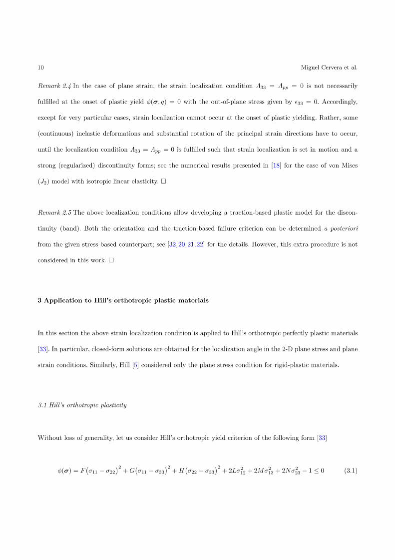
Remark 2.4 In the case of plane strain, the strain localization condition Λ33 = Λpp = 0 is not necessarily
fulfilled at the onset of plastic yield φ(σ, q) = 0 with the out-of-plane stress given by ε33 = 0. Accordingly,
except for very particular cases, strain localization cannot occur at the onset of plastic yielding. Rather, some
(continuous) inelastic deformations and substantial rotation of the principal strain directions have to occur,
until the localization condition Λ33 = Λpp = 0 is fulfilled such that strain localization is set in motion and a
strong (regularized) discontinuity forms; see the numerical results presented in [18] for the case of von Mises
(J2) model with isotropic linear elasticity.
Remark 2.5 The above localization conditions allow developing a traction-based plastic model for the discon-
tinuity (band). Both the orientation and the traction-based failure criterion can be determined a posteriori
from the given stress-based counterpart; see [32,20,21,22] for the details. However, this extra procedure is not
considered in this work.
3 Application to Hill’s orthotropic plastic materials
In this section the above strain localization condition is applied to Hill’s orthotropic perfectly plastic materials
[33]. In particular, closed-form solutions are obtained for the localization angle in the 2-D plane stress and plane
strain conditions. Similarly, Hill [5] considered only the plane stress condition for rigid-plastic materials.
3.1 Hill’s orthotropic plasticity
Without loss of generality, let us consider Hill’s orthotropic yield criterion of the following form [33]
φ(σ) = F(σ11 − σ22
)2+G
(σ11 − σ33
)2+H
(σ22 − σ33
)2+ 2Lσ2
12 + 2Mσ213 + 2Nσ2
23 − 1 ≤ 0 (3.1)

Strain localization analysis of Hill’s orthotropic elastoplasticity 11
with the material parameters F,G,H,L,M and N given by
F =1
2
[(1
σY,11
)2
+
(1
σY,22
)2
−(
1
σY,33
)2], L =
1
2
(1
σY,12
)2
(3.2a)
G =1
2
[(1
σY,11
)2
+
(1
σY,33
)2
−(
1
σY,22
)2], M =
1
2
(1
σY,13
)2
(3.2b)
H =1
2
[(1
σY,22
)2
+
(1
σY,33
)2
−(
1
σY,11
)2], N =
1
2
(1
σY,23
)2
(3.2c)
where σ11, σ22, σ33, σ12, σ13 and σ23 denote the stress components in the material local axes (1, 2, 3), with those
entities embellished by subscripts “Y ” representing the corresponding yield strengths.
The components Λij of the flow tensor Λ := dφ/dσ are then expressed as
Λ11 =dφ
dσ11= 2(F +G
)σ11 − 2Fσ22 − 2Gσ33 (3.3a)
Λ22 =dφ
dσ22= 2(F +H
)σ22 − 2Fσ11 − 2Hσ33 (3.3b)
Λ33 =dφ
dσ33= 2(G+H
)σ33 − 2Gσ11 − 2Hσ22 (3.3c)
Λ12 = Λ21 =1
2
dφ
dσ12= 2Lσ12 (3.3d)
Λ13 = Λ31 =1
2
dφ
dσ13= 2Mσ13 (3.3e)
Λ23 = Λ32 =1
2
dφ
dσ23= 2Nσ23 (3.3f)
Note that the identity trΛ = Λ11+Λ22+Λ33 = 0 always holds. That is, Hill’s yield function leads to an isochoric
(purely deviatoric) plastic flow.
Remark 3.1 von Mises’s isotropic yield criterion is recovered for
F = G = H =1
2
(1
σY
)2
, L = M = N =3
2
(1
σY
)2
(3.4)
for the yield strength σY .
3.2 Localization angles
In this section strain localization of a 2-D Hill’s plastic solid Ω ⊂ R2 is considered. In such 2-D cases, the
discontinuity orientation can be characterized by the inclination angle (counter-clockwise) θ ∈ [−π/2, π/2]
12 Miguel Cervera et al.
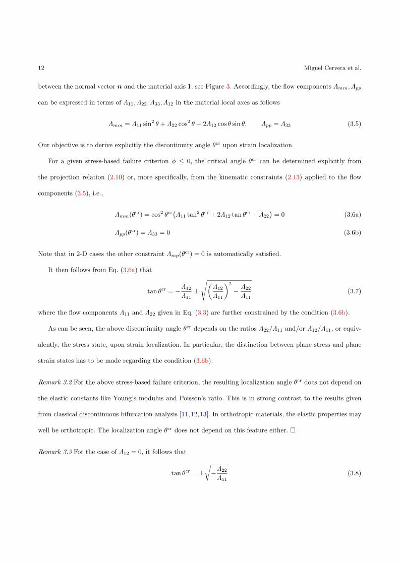
between the normal vector n and the material axis 1; see Figure 3. Accordingly, the flow components Λmm, Λpp
can be expressed in terms of Λ11, Λ22, Λ33, Λ12 in the material local axes as follows
Λmm = Λ11 sin2 θ + Λ22 cos2 θ + 2Λ12 cos θ sin θ, Λpp = Λ33 (3.5)
Our objective is to derive explicitly the discontinuity angle θcr upon strain localization.
For a given stress-based failure criterion φ ≤ 0, the critical angle θcr can be determined explicitly from
the projection relation (2.10) or, more specifically, from the kinematic constraints (2.13) applied to the flow
components (3.5), i.e.,
Λmm(θcr) = cos2 θcr(Λ11 tan2 θcr + 2Λ12 tan θcr + Λ22
)= 0 (3.6a)
Λpp(θcr) = Λ33 = 0 (3.6b)
Note that in 2-D cases the other constraint Λmp(θcr) = 0 is automatically satisfied.
It then follows from Eq. (3.6a) that
tan θcr = −Λ12
Λ11±√(
Λ12
Λ11
)2
− Λ22
Λ11(3.7)
where the flow components Λ11 and Λ22 given in Eq. (3.3) are further constrained by the condition (3.6b).
As can be seen, the above discontinuity angle θcr depends on the ratios Λ22/Λ11 and/or Λ12/Λ11, or equiv-
alently, the stress state, upon strain localization. In particular, the distinction between plane stress and plane
strain states has to be made regarding the condition (3.6b).
Remark 3.2 For the above stress-based failure criterion, the resulting localization angle θcr does not depend on
the elastic constants like Young’s modulus and Poisson’s ratio. This is in strong contrast to the results given
from classical discontinuous bifurcation analysis [11,12,13]. In orthotropic materials, the elastic properties may
well be orthotropic. The localization angle θcr does not depend on this feature either.
Remark 3.3 For the case of Λ12 = 0, it follows that
tan θcr = ±√−Λ22
Λ11(3.8)
Strain localization analysis of Hill’s orthotropic elastoplasticity 13
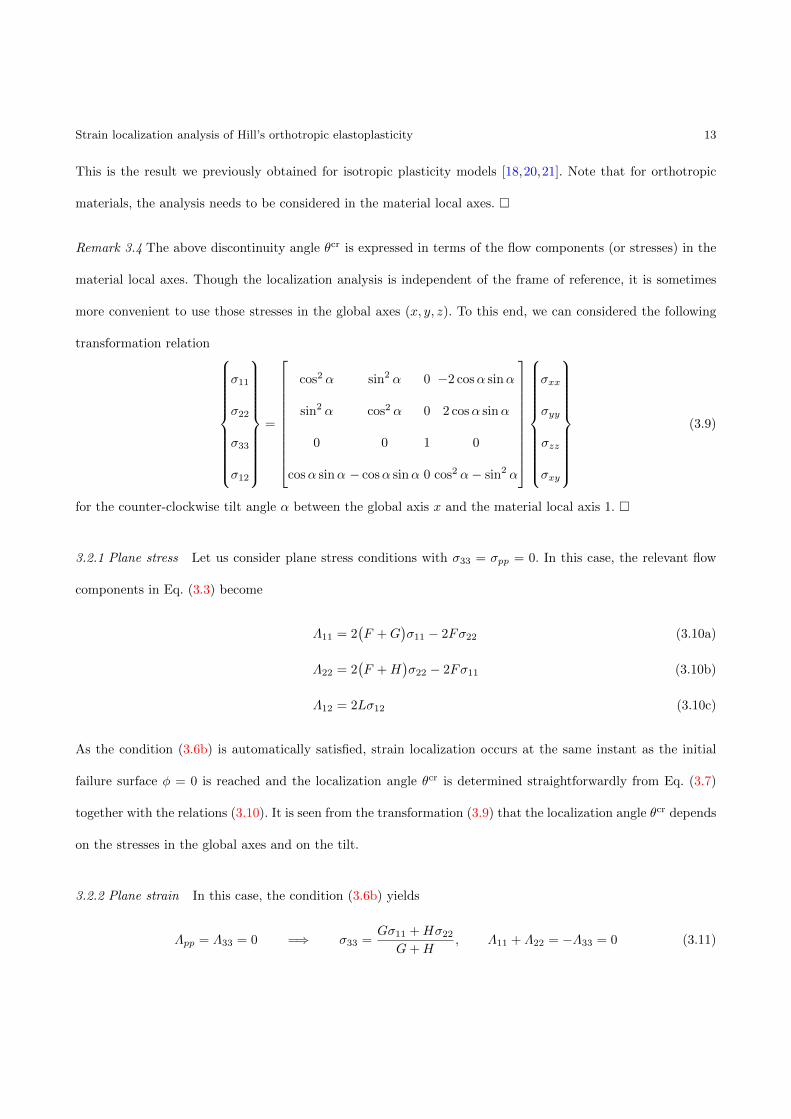
This is the result we previously obtained for isotropic plasticity models [18,20,21]. Note that for orthotropic
materials, the analysis needs to be considered in the material local axes.
Remark 3.4 The above discontinuity angle θcr is expressed in terms of the flow components (or stresses) in the
material local axes. Though the localization analysis is independent of the frame of reference, it is sometimes
more convenient to use those stresses in the global axes (x, y, z). To this end, we can considered the following
transformation relation
σ11
σ22
σ33
σ12
=
cos2 α sin2 α 0 −2 cosα sinα
sin2 α cos2 α 0 2 cosα sinα
0 0 1 0
cosα sinα − cosα sinα 0 cos2 α− sin2 α
σxx
σyy
σzz
σxy
(3.9)
for the counter-clockwise tilt angle α between the global axis x and the material local axis 1.
3.2.1 Plane stress Let us consider plane stress conditions with σ33 = σpp = 0. In this case, the relevant flow
components in Eq. (3.3) become
Λ11 = 2(F +G
)σ11 − 2Fσ22 (3.10a)
Λ22 = 2(F +H
)σ22 − 2Fσ11 (3.10b)
Λ12 = 2Lσ12 (3.10c)
As the condition (3.6b) is automatically satisfied, strain localization occurs at the same instant as the initial
failure surface φ = 0 is reached and the localization angle θcr is determined straightforwardly from Eq. (3.7)
together with the relations (3.10). It is seen from the transformation (3.9) that the localization angle θcr depends
on the stresses in the global axes and on the tilt.
3.2.2 Plane strain In this case, the condition (3.6b) yields
Λpp = Λ33 = 0 =⇒ σ33 =Gσ11 +Hσ22
G+H, Λ11 + Λ22 = −Λ33 = 0 (3.11)

14 Miguel Cervera et al.
Accordingly, Eq. (3.7) becomes
tan θcr = −Λ12
Λ11±√(
Λ12
Λ11
)2
+ 1 (3.12)
where the flow components are expressed as
Λ11 = −Λ22 = 2FG+ FH +GH
G+H
(σ11 − σ22
), Λ12 = 2Lσ12 (3.13)
or, equivalently,
Λ12
Λ11=
(G+H
)L
FG+ FH +GH· σ12σ11 − σ22
(3.14)
Therefore, the localization angle θcr depends on the ratio σ12/(σ11 − σ22); see Remark 3.7.
Remark 3.5 It follows from Eq. (3.12) that
tan θcr1 · tan θcr2 = −1 =⇒∣∣θcr1 − θcr2 ∣∣ = 90 (3.15)
Accordingly, the discontinuity lines are perpendicular to each other.
Remark 3.6 For the case of Λ12 = 0, Eq. (3.12) becomes
tan θcr = 1 =⇒ θcr = ±45 (3.16)
This is exactly the result obtained for isotropic plasticity [18,20,21].
Remark 3.7 It follows from the transformation (3.9) that
σ12σ11 − σ22
=1
2
(σxx − σyy
)sin(2α) + 2σxy cos(2α)(
σxx − σyy)
cos(2α)− 2σxy sin(2α)(3.17)
Regarding the stresses in the global axes, the following two cases are of interest
σ12σ11 − σ22
=
1
2tan(2α) σxy = 0
1
2 tan(2α)σxx = σyy
(3.18)
In the first case, the principal directions are aligned with the global axes, while in the second one, they are at
45 with respect to the global reference. In both cases, the localization angle θcr depends only on the tilt angle
α of the material axes.

Strain localization analysis of Hill’s orthotropic elastoplasticity 15
3.3 Particular examples
In order to make the above results more clear, let us consider the stress state of vertical stretching, i.e.,
σxx = 0, σyy = σ, σxy = 0 (3.19)
along axis y.
For the plane stress condition, it follows from Eqs. (3.9) and (3.10) that
Λ22
Λ11=
(F +H
)cos2 α− F sin2 α(
F +G)
sin2 α− F cos2 α(3.20a)
Λ12
Λ11= − L cosα sinα(
F +G)
sin2 α− F cos2 α(3.20b)
The localization angle θcr is then determined from Eq. (3.7). In particular, for the case α = 0, it follows that
tan θcr = ±√−Λ22
Λ11= ±
√F +H
F(3.21)
which depends only on the material plastic parameters F and H. This result is coincident with that in [5]
obtained from the “zero rate of extension”.
For the plane strain condition, the localization angle θcr is determined from Eq. (3.12)
Λ12
Λ11=
1
2
(G+H
)L
FG+ FH +GHtan(2α) (3.22)
For the case α = 0, it follows that
tan θcr = ±1 =⇒ θcr = ±45 (3.23)
4 Numerical verifications
In this section the analytical results presented in Section 3 are numerically verified. It is stressed that the
numerical verification is totally independent from the analytical results. That is, these results are not used in
any way in finite element simulations. Perfect plasticity with null modulus H = 0 is considered in this work,
though the present strain localization analysis applies also to plastic-damage models with softening regimes.

16 Miguel Cervera et al.
This is because the equations from which the localization angle is obtained, Eq. (2.13) and Eq. (3.7), depend
only on the plastic flow components in the material local system; they do not depend on the softening modulus.
Compelling results for isotropic elastoplastic models with softening regimes are shown in reference [21].
As seen in previous Sections, Hill’s plastic flow is isochoric by definition, and for strain localization to take
place the plastic flow needs to be well developed and, at that stage, the (incompressible) plastic component
of the deformation is dominant over the elastic part. Standard displacement-based finite elements are not well
suited to cope with this quasi-incompressibility situation and this blunder is more evident if low order finite
elements are used. Mixed displacement/pressure (u/p) finite element formulations are far more suitable to tackle
(quasi)-incompressible problems [34]. In previous works, the authors have used mixed displacement-pressure
elements [35,18] and strain-displacement ones [22] in the solution of strain localization problems in isochoric
and quasi-isochoric situations.
In this work, orthotropic elasticity is addressed as well as orthotropic plasticity. In orthotropic elasticity, two
interesting questions arise in contrast to isotropic elasticity. On the one hand, there is no simple scalar relation
between the pressure (or mean stress) and the volumetric strain. This renders inapplicable most developments
related to mixed u/p formulations. This is also the case of some related elements, like the widely used Q1P0,
where the discontinuous constant pressure is eliminated at element level to yield a final formulation in terms of
displacements only. On the other hand, the term “incompressible material” results a contentious matter when
referred to anisotropic solids, see [36] for a discussion on this subject. Fortunately, the B-bar method can be
introduced to deal with anisotropic and non-linear media [37,38]. This method is adopted in this work.
4.1 B-bar finite element
In the standard displacement based finite element method, the strain field ε inside an element is related to the
nodal displacements a by the strain-displacement matrix B (discrete symmetric gradient operator)
ε = Ba (4.1)
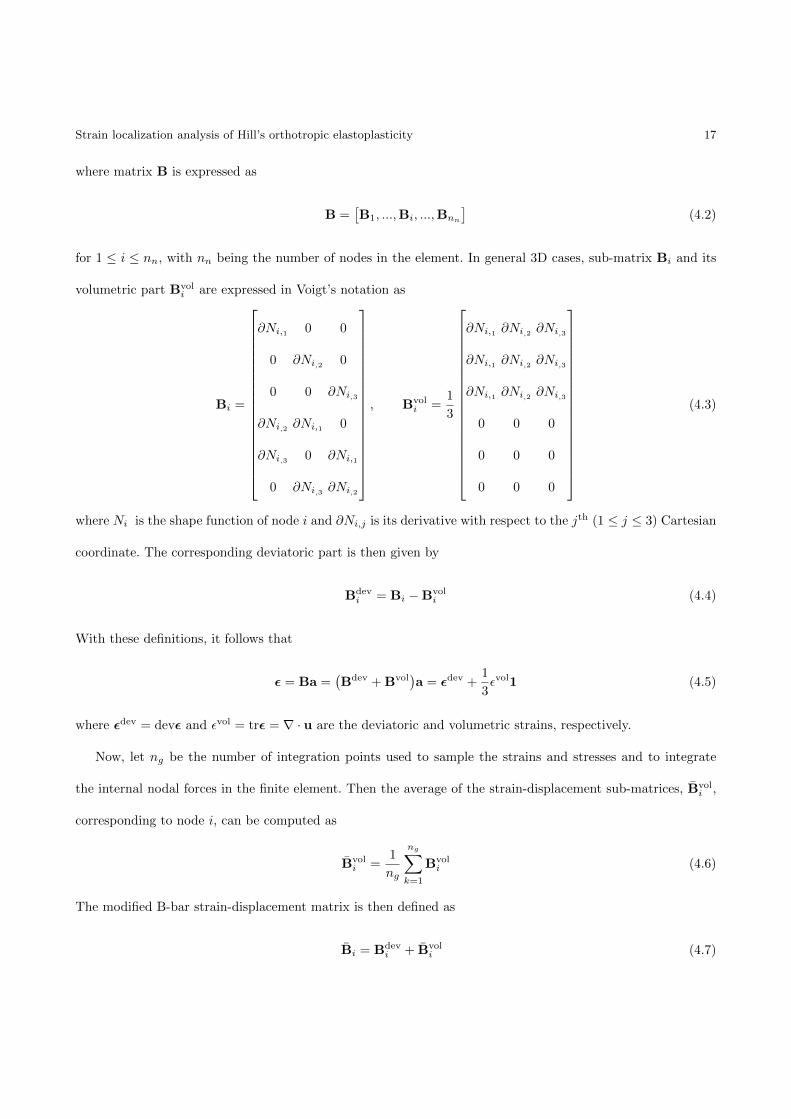
Strain localization analysis of Hill’s orthotropic elastoplasticity 17
where matrix B is expressed as
B =[B1, ...,Bi, ...,Bnn
](4.2)
for 1 ≤ i ≤ nn, with nn being the number of nodes in the element. In general 3D cases, sub-matrix Bi and its
volumetric part Bvoli are expressed in Voigt’s notation as
Bi =
∂Ni,1 0 0
0 ∂Ni,2 0
0 0 ∂Ni,3
∂Ni,2 ∂Ni,1 0
∂Ni,3 0 ∂Ni,1
0 ∂Ni,3 ∂Ni,2
, Bvoli =
1
3
∂Ni,1 ∂Ni,2 ∂Ni,3
∂Ni,1 ∂Ni,2 ∂Ni,3
∂Ni,1 ∂Ni,2 ∂Ni,3
0 0 0
0 0 0
0 0 0
(4.3)
where Ni is the shape function of node i and ∂Ni,j is its derivative with respect to the jth (1 ≤ j ≤ 3) Cartesian
coordinate. The corresponding deviatoric part is then given by
Bdevi = Bi −Bvol
i (4.4)
With these definitions, it follows that
ε = Ba =(Bdev + Bvol
)a = εdev +
1
3εvol1 (4.5)
where εdev = devε and εvol = trε = ∇ · u are the deviatoric and volumetric strains, respectively.
Now, let ng be the number of integration points used to sample the strains and stresses and to integrate
the internal nodal forces in the finite element. Then the average of the strain-displacement sub-matrices, Bvoli ,
corresponding to node i, can be computed as
Bvoli =
1
ng
ng∑k=1
Bvoli (4.6)
The modified B-bar strain-displacement matrix is then defined as
Bi = Bdevi + Bvol
i (4.7)
18 Miguel Cervera et al.
As explained in [37], the B-bar method is equivalent to the use of reduced integration for the volumetric part of
the strain energy, while full integration is retained for the deviatoric contribution. Under given circumstances,
a B-bar Q1 element is identical to the mixed Q1P0 element, but obtained through the deviatoric/volumetric
split of the strains rather than the stresses.
4.2 Example: Strip under vertical stretching
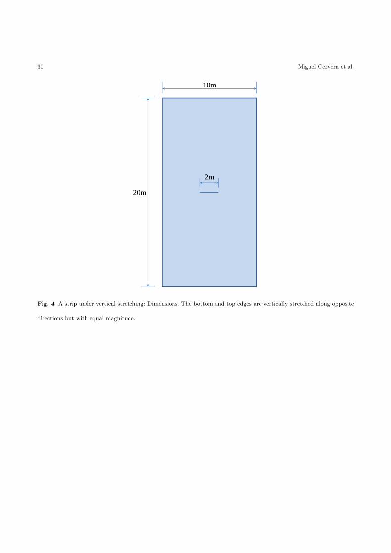
In this section, a strip under vertical stretching is considered as shown in Figure 4. Following Hill [5] where
characteristics are defined as “curves along which small disturbances propagates, a sharp horizontal slit is
inserted in the strip to introduce the perturbation necessary to trigger strain localization. The far field stress
state corresponds exactly to that given in Eq. (3.19). The analytical results presented in Section 3.3 are compared
to the corresponding numerical ones.
4.2.1 Isotropic and orthotropic elasticity with von Mises plasticity. Let us consider the reference material of
J2 perfect plasticity, and isotropic elastic behavior with Young’s modulus E0 = 1.0× 10⁷ MPa, Poisson’s ratio
ν0 = 0.2 and the yield strength σY = 1.0× 10⁴ MPa.
Due to the facts σ12 = 0 and Λ12 = 0, the localization angle is given from Eq. (3.8), i.e.,
tan θcr =
±√
2 Plane stress
±1 Plane strain
=⇒ θcr =
±54.74 Plane stress
±45 Plane strain
(4.8)
The above results were obtained and numerically validated in previous works [18,21].
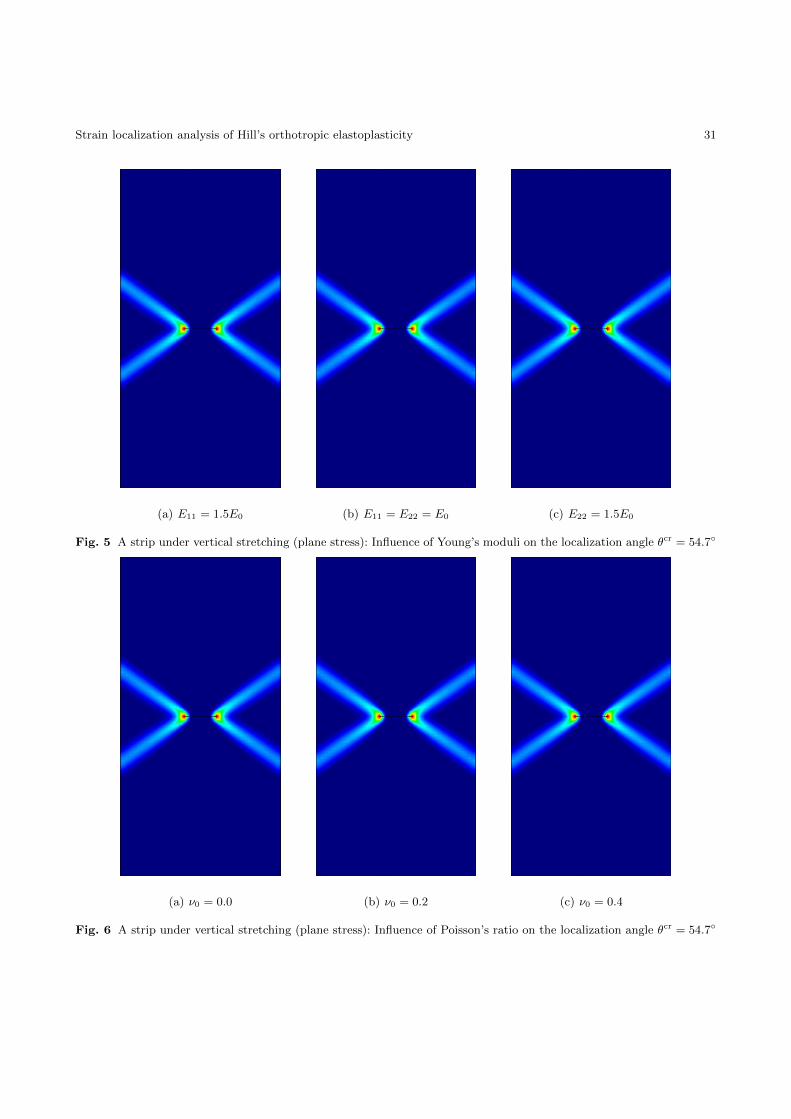
As shown in Figures 5 and 6 for the plane stress cases and Figures 7 and 8 for the plane strain cases, the
localization angle θcr depends neither on Young’s modulus nor on Poisson’s ratio, even if they are varied in an
orthotropic fashion.
4.2.2 Othotropic Hill material with no tilt. The Hill orthotropic plasticity material with the local axis 1 coin-
cident with the global one x, i.e., α = 0, is considered. In this case, the analytical localization angle θcr is given
by Eqs. (3.21) and (3.23), respectively.
Strain localization analysis of Hill’s orthotropic elastoplasticity 19
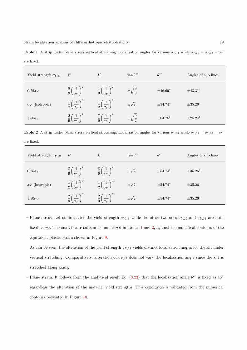
Table 1 A strip under plane stress vertical stretching: Localization angles for various σY,11 while σY,22 = σY,33 = σY
are fixed.
Yield strength σY,11 F H tan θcr θcr Angles of slip lines
0.75σY8
9
(1
σY
)21
9
(1
σY
)2
±√
9
8±46.69 ±43.31
σY (Isotropic)1
2
(1
σY
)21
2
(1
σY
)2
±√
2 ±54.74 ±35.26
1.50σY2
9
(1
σY
)27
9
(1
σY
)2
±√
9
2±64.76 ±25.24
Table 2 A strip under plane stress vertical stretching: Localization angles for various σY,22 while σY,11 = σY,33 = σY
are fixed.
Yield strength σY,22 F H tan θcr θcr Angles of slip lines
0.75σY8
9
(1
σY
)28
9
(1
σY
)2
±√
2 ±54.74 ±35.26
σY (Isotropic)1
2
(1
σY
)21
2
(1
σY
)2
±√
2 ±54.74 ±35.26
1.50σY2
9
(1
σY
)22
9
(1
σY
)2
±√
2 ±54.74 ±35.26
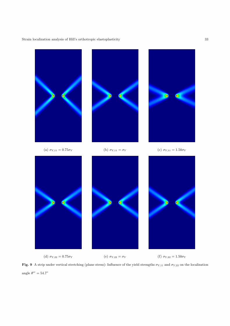
– Plane stress: Let us first alter the yield strength σY,11 while the other two ones σY,22 and σY,33 are both
fixed as σY . The analytical results are summarized in Tables 1 and 2, against the numerical contours of the
equivalent plastic strain shown in Figure 9.
As can be seen, the alteration of the yield strength σY,11 yields distinct localization angles for the slit under
vertical stretching. Comparatively, alteration of σY,22 does not vary the localization angle since the slit is
stretched along axis y.
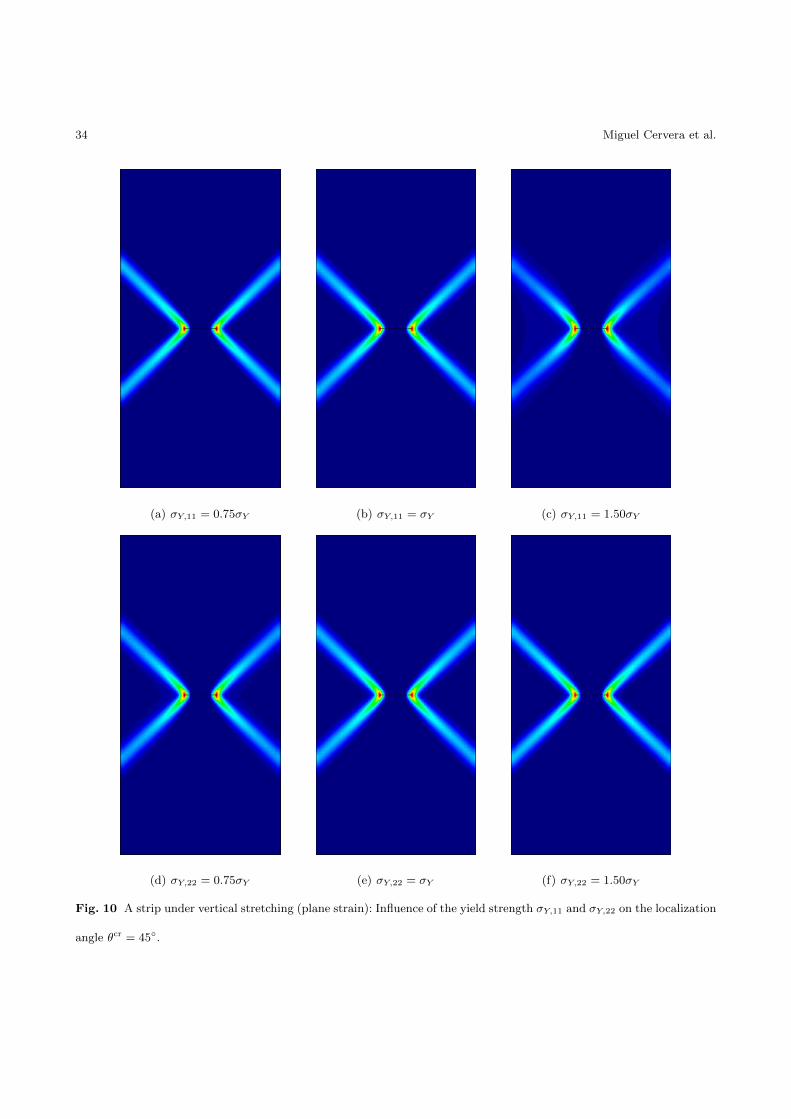
– Plane strain: It follows from the analytical result Eq. (3.23) that the localization angle θcr is fixed as 45
regardless the alteration of the material yield strengths. This conclusion is validated from the numerical
contours presented in Figure 10.

20 Miguel Cervera et al.
For all cases, the analytical results are coincident with the numerical ones as expected.
4.2.3 Othotropic Hill material with tilt. Let us now discuss the Hill orthotropic plasticity with the material
local axis 1 different from the global one x, i.e., α 6= 0. Similarly, the plane stress and plane strain conditions
have to be discriminated.
– Plane stress: The analytical localization angle θcr is given by Eq. (3.7) together with the ratios (3.20). In
particular, some analytical results are summarized in Tables 3, 4, 5 and 6. The numerical contours of the
equivalent plastic strain are shown in Figures 11 to 14.
As can be seen, variation of the yield strengths in both directions yields distinct localization angles.
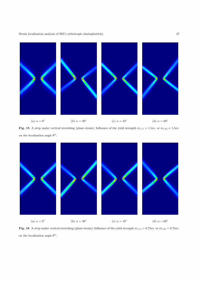
– Plane strain: Some of the analytical localization angles θcr given by Eq. (3.12) together with the ratios (3.22)
are summarized in Tables 7 and 8. The corresponding numerical contours of the equivalent plastic strain are
shown in Figures 15 and 16.
Compared to the results of plane stress, the variation of the yield strength in both directions has the same
influences on the localization angles.
In all cases, the analytical results are reproduced by the numerical ones. Note again that the above results
given from localization analyses are independent of the frame of reference. However, if the material axes are
not aligned with the direction of straining, the strip is no longer of uniaxial straining in the material axes.
Accordingly, considering material tilting with respect to the direction of straining verifies the results obtained
for multi-directional straining.
4.3 Example: Indentation by a flat rigid die
The second example is the indentation by a flat rigid die shown in Figure 17. This is a well-known 2-D plane
strain problem usually used in the literature to test the ability of plasticity model to capture the failure modes;
see also [5].

Strain localization analysis of Hill’s orthotropic elastoplasticity 21
Table 3 A strip under plane stress vertical stretching: Localization angles for σY,11 = 1.50σY at various tilts α.
Tilt α tan θcr θcr θcr + α Angles of slip lines
0 −2.1213; 2.1213 64.8; −64.8 64.8; −64.8 −25.2; 25.2
30 −23.906; 0.5229 −87.6; 27.6 57.6; −57.6 −32.4; 32.4
45 0.2644; 13.236 14.8; 85.7 59.8; 130.7 −30.2; 40.7
60 0.0651; 4.6115 3.7; 77.8 63.7; 137.8 −26.3; 47.8
Table 4 A strip under plane stress vertical stretching: Localization angles for σY,11 = 0.75σY at various tilts α.
Tilt α tan θcr θcr θcr + α Angles of slip lines
0 −1.0607; 1.0607 46.7; −46.7 46.7; −46.7 −43.3; 43.3
30 −6.2271; 0.3814 −80.9; 20.9 50.9; −50.9 −39.1; 39.1
45 0.0375; 3.3375 2.1; 73, 3 47.1; 118.3 −42.9; 28.3
60 −0.2620; 1.4312 −14.7; 55.1 45.3; 115.1 −44.7; 25.1
Table 5 A strip under plane stress vertical stretching: Localization angles for σY,22 = 1.50σY at various tilts α.
Tilt α tan θcr θcr θcr + α Angles of slip lines
0 −1.1414; 1.1414 54.7; −54.7 54.7; −54.7 −35.3; 35.3
30 0.2169; 15.3716 12.2; 86.3 42.2; 116.3 −47.8; 26.3
45 0.0756; 3.7816 4.3; 75.2 49.3; 120.2 −40.7; 30.2
60 −0.0418; 1.9124 −2.4; 62.4 57.6; 122.4 −32.4; 32.4
Table 6 A strip under plane stress vertical stretching: Localization angles for σY,22 = 0.75σY at various tilts α.
Tilt α tan θcr θcr θcr + α Angles of slip lines
0 −1.1414; 1.1414 54.7; −54.7 54.7; −54.7 −35.3; 35.3
30 −3.8164; 0.6987 −75.3; 34.9 −45.3; 64.9 44.7; −25.1
45 0.2996; 26.700 16.7; 87.9 61.7; 132.9 −28.3; 42.9
60 −0.1606; 2.6219 −9.1; 69.1 50.9; 129.1 39.1; 39.1

22 Miguel Cervera et al.
Table 7 A strip under plane strain vertical stretching: Localization angles for σY,11 = 1.50σY or σY,22 = 1.50σY at
various tilts α.
Tilt α tan θcr θcr θcr + α Angles of slip lines
0 −1.0000; 1.0000 45.0; −45.0 45.0; −45.0 −45.0; 45.0
30 −6.7251; 0.1487 −81.5; 8.5 −51.5; 38.5 38.5; −51.5
45 0; −∞ 0.0; −90.0 45.0; −45.0 −45.0; 45.0
60 −0.1487; 6.7251 −8.5; 81.5 51.5; 141.5 −38.5; 51.5
Table 8 A strip under plane strain vertical stretching: Localization angles for σY,11 = 0.75σY or σY,22 = 0.75σY at
various tilts α.
Tilt α tan θcr θcr θcr + α Angles of slip lines
0 −1.0000; 1.0000 45.0; −45.0 45.0; −45.0 −45.0; 45.0
30 −2.9675; 0.3370 −71.4; 18.6 −41.4; 48.6 48.6; −41.4
45 0; −∞ 0.0; −90.0 45.0; −45.0 −45.0; 45.0
60 −0.3370; 2.9675 −18.6; 71.4 41.4; 131.4 −48.6; 41.4
As shown in Figure 18, the material right under the rigid die is almost under uniaxial vertical loading in
the global axes, i.e., σxy = 0. In accordance with Remark 3.7, the localization angle θcr is determined from Eq.
(3.12) with the following ratio
Λ12
Λ11=
1
2
(G+H
)L
FG+ FH +GHtan(2α) (4.9)
for the tilt α.

Strain localization analysis of Hill’s orthotropic elastoplasticity 23
4.3.1 Isotropic von Mises material. Similarly as before, let us first consider the reference isotropic material of
J2 perfect plasticity, with Young’s modulus E0 = 1.0×10⁷ MPa, Poisson’s ratio ν0 = 0.2 and the yield strength
σY = 1.0× 10⁴ MPa.
As shown in Figure 19, the localization angle is fixed θcr = 45 regardless of the elastic constants. It is
worthy noting that the failure modes are symmetric and corresponds to the claimed Prandtl’s solution.
4.3.2 Orthotropic Hill material with no tilt. It follows from α = 0 that Λ12/Λ11 = 0. Accordingly, the local-
ization angle is also fixed as θcr = 45 regardless of the material yield strength; see Figure 20 for the numerical
results.
4.3.3 Orthotropic Hill material with tilt. As the localization angle depends only on the tilt, regardless of the
stresses, the results coincide with those for the slit under plane strain vertical stretching. Therefore, the analytical
localization angles summarized in Tables 7 and 8 also apply here. The numerical results presented in Figures
21 and 22 validate this conclusion.
As can be seen, due to the tilt of the material axes the failure modes are no longer symmetric. Note that
the results for α = 45 are identical to those for α = 0 and the results for α = 30 are symmetric to those for
α = 60 in both figures.
Note that in all cases the obtained results agree with those of Hill [5] for rigid-plastic materials.
5 Conclusions
In this work the strain localization analysis of Hill’s orthotropic plasticity is addressed. Similarly to our previous
work on isotropic plastic or damage models, the localization condition is derived from the boundedness of stress
rates together with Maxwell’s kinematics. That is, the plastic flow components perpendicular to the discontinuity
normal vector vanish upon strain localization. Compared to the classical work based on the discontinuous
bifurcation analysis, in the material axes the localization angles are independent from the elastic constants, but
rather, they depend exclusively on the material parameters involved in the plastic yield function. This turns out

24 Miguel Cervera et al.
to be coincident with Hill’s results for strictly incompressible rigid-plastic problems, extending them to general
elasto-plastic materials.
In 2-D plane stress and plane strain situations, application of the above localization condition to Hill’s
orthotropic plasticity yields closed-form solutions of the localization angles. In particular, the discontinuity lines
in plane strain conditions are always perpendicular to each other, and the localization angle depends only on
the tite angle of the material axes for the case of shear stress free states.
The analytical results are validated independently by numerical simulations. Being the plastic flow purely
isochoric, the B-bar finite element is employed to deal with the incompressibility of the plastic flow. Regarding a
horizontal slit under vertical stretching and Prandtl’s punch test in plane strain, numerical results are presented
for both the isotropic plasticity and the orthotropic one with or without tilt angle between the material axes
and the global ones. In all cases, the critical angles predicted from the localization condition coincide with those
given by numerical simulations. Interestingly, as for Prandtl’s punch test in plane strain the material right under
the rigid footing is almost free of shear stresses, the localization angles are also independent from the stress
state and can be determined as those for a slit under vertical stretching.
6 Acknowledgments
Financial support from the Spanish Government-MINECO-Proyectos de I + D (Excelencia)-DPI2017-85998-P-
ADaMANT-Computational Framework for Additive Manufacturing of Titanium Alloy and the Catalan Govern-
ment ACCIO - Ris3cat Transport and PRO2 Project is gratefully acknowledged. This work is also supported
by the National Natural Science Foundation of China (51878294; 51678246), the State Key Laboratory of
Subtropical Building Science (2018ZC04) and the Funding for Central Universities (2018PY20) to J.Y. Wu.
References
1. L. Prandtl. Uber die haete plastistischer korper. Nachr. Ges. Wisensch, Gottingen, math. phys. Klasse, pages 74–85,
1920.
Strain localization analysis of Hill’s orthotropic elastoplasticity 25
2. H. Hencky. Uber einige statisch bestimmte falle des gleichgewichts in plastischen korpern. Z. Angew. Math. Mech.,
3:241–251, 1923.
3. H. Hencky. Zur theorie plastischer deformationen und der hierdurch im material hervorgerufenen nachspannungen.
Z. Angew. Math. Mech., 4:323–334, 1924.
4. J. Mandel. Equilibre par trasches planes des solides a la limite d’ecoulement. PhD thesis, These, Paris, 1942.
5. R. Hill. The Mathematical Theory of Plasticity. Oxford University Press, New York, 1950.
6. R. Hill. On discontinuous plastic states, with special reference to localized necking in thin sheets. J. Mech. Phys.
Solids, 1:19–30, 1952.
7. R. Hill. General theory of uniqueness and stability of elasto-plastic solids. J. Mech. Phys. Solids, 6:236–249, 1958.
8. R. Hill. Acceleration waves in solids. J. Mech. Phys. Solids, 10:1–16, 1962.
9. T.Y. Thomas. Plastic Flow and Fracture of Solids. Academic Press, New York, 1961.
10. J. R. Rice. A path independent integral and the approximate analysis of strain cncentrations by notches and cracks.
J. Appl. Mech.-T. ASME, 35:379–386, 1968.
11. J. W. Rudnicki and J. R. Rice. Conditions of the localization of deformation in pressure-sensitive dilatant material.
J. Mech. Phys. Solids, 23:371–394, 1975.
12. J. R. Rice and J. W. Rudnicki. A note on some features of the theory of localization of deformation. Int. J. Solids
Structures, 16:597–605, 1980.
13. K. Runesson, N.S. Ottosen, and D. Peric. Discontinuous bifurcations of elastic-plastic solutions at plane stress and
plane strain. Int. J. Plast., 7:99–121, 1991.
14. J.C. Simo, J. Oliver, and F. Armero. An analysis of strong discontinuities induced by strain-softening in rate-
independent inelastic solids. Comput. Mech., 12:277–296, 1993.
15. J. Oliver. Modeling strong discontinuities in solid mechanics via strain softening constitutive equations. part i:
Fundamentals; part ii: Numerical simulation. International Journal for Numerical Methods in Engineering, 39:3575–
3600; 3601–3623, 1996.
16. J. Oliver, M. Cervera, and O. Manzoli. Strong discontinuities and continuum plasticity models: the strong disconti-
nuity approach. Int. J. Plast., 15:319–351, 1999.
17. J. Oliver. On the discrete constitutive models induced by strong discontinuity kinematics and continuum constitutive
equations. International Journal of Solids and Structures, 37:7207–7229, 2000.

26 Miguel Cervera et al.
18. M. Cervera, M. Chiumenti, and D. Di Capua. Benchmarking on bifurcation and localization in j2 plasticity for plane
stress and plane strain conditions. Comput. Methods Appl. Mech. Eng., 241244:206224, 2012.
19. J. Oliver, A. E. Huespe, and I. F. Dias. Strain localization, strong discontinuities and material fracture: Matches and
mismatches. Comput. Methods Appl. Mech. Eng., 241:323–336, 2006.
20. J. Y. Wu and M. Cervera. On the equivalence between traction- and stress-based approaches for the modeling of
localized failure in solids. Journal of the Mechanics and Physics of Solids, 82:137–163, 2015.
21. J. Y. Wu and M. Cervera. A thermodynamically consistent plastic-damage framework for localized failure in quasi-
brittle solids: Material model and strain localization analysis. International Journal of Solids and Structures, 88-
89:227–247, 2016.
22. J. Y. Wu and M. Cervera. Strain localization of elastic-damaging frictional-cohesive materials: Analytical results and
numerical verification. Materials, 10:434; doi:10.3390/ma10040434, 2017.
23. M. Cervera, M. Chiumenti, L. Benedetti, and R. Codina. Mixed stabilized finite element methods in nonlinear solid
mechanics. part iii: Compressible and incompressible plasticity. Comput. Methods Appl. Mech. Eng., 285:752–775,
2015.
24. O. Hoffman. The brittle strength of orthotropic materials. J. Comp. Mater., 1:200–206, 1967.
25. S. W. Tsai and E. M. Wu. A general theory of strength for anisotropic materials. J. Comp. Mater., 5:58–80, 1971.
26. S. Oller, E. Car, and J. Lubliner. Definition of a general implicit orthotropic yield criterion. Comput. Methods Appl.
Mech. Engrg., 192:895–912, 2003.
27. M. Li, J. Fussl, M. Lukacevic, and J. Eberhardsteiner. A numerical upper bound formulation with sensibly-arranged
velocity discontinuities and orthotropic material strength behavior. Journal of Theoretical and Applied Mechanics,
56(2):417–433, 2018.
28. J.G. Rots, P. Nauta, G.M.A. Kusters, and J. Blaauwendraad. Smeared crack approach and fracture localization in
concrete. Heron, 30:1–47, 1985.
29. M. Jirasek and T. Zimmermann. Analysis of rotating crack model. J. Eng. Mech., ASCE, 124(8):842–851, 1998.
30. M. Cervera. A smeared-embedded mesh-corrected damage model for tensile cracking. Int. J. Numer. Meth. Engng.,
76:1930–1954, 2008.
31. M. Cervera. An orthotropic mesh corrected crack model. Comput. Methods Appl. Mech. Engrg., 197:1603–1619, 2008.

Strain localization analysis of Hill’s orthotropic elastoplasticity 27
32. J. Y. Wu and M. Cervera. Strain localization and failure mechanics for elastoplastic damage solids. Monograph
CIMNE M147, Barrcelona, Spain, 2014.
33. R. Hill. A theory of the yielding and plastic flow of anisotropic metals. Proc. Roy. Soc. A, 193:281–297, 1948.
34. J.C. Simo and T.J.R. Hughes. Computational inelasticity. Springer, New York, 1998.
35. M. Cervera and M. Chiumenti. Size effect and localization in j2 plasticity. International Journal of Solids and
Structures, 46:3301–3312, 2009.
36. C. A. Felippa and E. Onate. Stress, strain and energy splittings for anisotropic solids under volumetric constraints.
Computers & Structures, 81(13):1343–1357, 2003.
37. T. J. R. Hughes. Generalization of selective intertegration procedures to anisotropic and nonlinear media. Interna-
tional Journal for Numerical Methods in Engineering, 15(9):1413–1418, 1980.
38. T.R.J. Hughes. The finite element method. Linear Static and Dynamic Finite Element Analysis. Dover Publications
Inc., Mineaola, New York, 2000.

28 Miguel Cervera et al.
S
Ω+
Ω−
xS
n
(a) Strong discontinuity
SS−
S+
Ω+
Ω−
xS
n
x∗S
b
(b) Regularized discontinuity
Fig. 1 Strong and regularized discontinuities in a solid
x
u
˙u(x)
w
x
ε
xS
xS
∇sym ˙u
(w ⊗ n)symδS
(a) Velocity/strain rate fields around a strong disconti-
nuity
x
u
˙u(x)
w
x
ε
xS
xS
∇sym ˙u
1
b(w ⊗ n)sym
b
(b) Velocity/strain rate fields around a regularized dis-
continuity
Fig. 2 Kinematics of strong and regularized discontinuities

Strain localization analysis of Hill’s orthotropic elastoplasticity 29
x
y
O
12
0
n
m
cr
Fig. 3 Definition of the localization angle θcr between the normal vector n of the discontinuity and the material local
axis 1.
30 Miguel Cervera et al.
10m
2m
20m
Fig. 4 A strip under vertical stretching: Dimensions. The bottom and top edges are vertically stretched along opposite
directions but with equal magnitude.
Strain localization analysis of Hill’s orthotropic elastoplasticity 31
(a) E11 = 1.5E0 (b) E11 = E22 = E0 (c) E22 = 1.5E0
Fig. 5 A strip under vertical stretching (plane stress): Influence of Young’s moduli on the localization angle θcr = 54.7
(a) ν0 = 0.0 (b) ν0 = 0.2 (c) ν0 = 0.4
Fig. 6 A strip under vertical stretching (plane stress): Influence of Poisson’s ratio on the localization angle θcr = 54.7

32 Miguel Cervera et al.
(a) E11 = 1.5E0 (b) E11 = E22 = E0 (c) E22 = 1.5E0
Fig. 7 A strip under vertical stretching (plane strain): Influence of Young’s moduli on the localization angle θcr = 45
(a) ν0 = 0.0 (b) ν0 = 0.2 (c) ν0 = 0.4
Fig. 8 A strip under vertical stretching (plane strain): Influence of Poisson’s ratio on the localization angle θcr = 45
Strain localization analysis of Hill’s orthotropic elastoplasticity 33
(a) σY,11 = 0.75σY (b) σY,11 = σY (c) σY,11 = 1.50σY
(d) σY,22 = 0.75σY (e) σY,22 = σY (f) σY,22 = 1.50σY
Fig. 9 A strip under vertical stretching (plane stress): Influence of the yield strengths σY,11 and σY,22 on the localization
angle θcr = 54.7
34 Miguel Cervera et al.
(a) σY,11 = 0.75σY (b) σY,11 = σY (c) σY,11 = 1.50σY
(d) σY,22 = 0.75σY (e) σY,22 = σY (f) σY,22 = 1.50σY
Fig. 10 A strip under vertical stretching (plane strain): Influence of the yield strength σY,11 and σY,22 on the localization
angle θcr = 45.

Strain localization analysis of Hill’s orthotropic elastoplasticity 35
(a) α = 0 (b) α = 30 (c) α = 45 (d) α = 60
Fig. 11 A strip under vertical stretching (plane stress): Influence of the yield strength σY,11 = 1.5σY on the localization
angle θcr.
(a) α = 0 (b) α = 30 (c) α = 45 (d) α = 60
Fig. 12 A strip under vertical stretching (plane stress): Influence of the yield strength σY,11 = 0.75σY on the localization
angle θcr.

36 Miguel Cervera et al.
(a) α = 0 (b) α = 30 (c) α = 45 (d) α = 60
Fig. 13 A strip under vertical stretching (plane stress): Influence of the yield strength σY,22 = 1.5σY on the localization
angle θcr.
(a) α = 0 (b) α = 30 (c) α = 45 (d) α = 60
Fig. 14 A strip under vertical stretching (plane stress): Influence of the yield strength σY,22 = 0.75σY on the localization
angle θcr.
Strain localization analysis of Hill’s orthotropic elastoplasticity 37
(a) α = 0 (b) α = 30 (c) α = 45 (d) α = 60
Fig. 15 A strip under vertical stretching (plane strain): Influence of the yield strength σY,11 = 1.5σY or σY,22 = 1.5σY
on the localization angle θcr.
(a) α = 0 (b) α = 30 (c) α = 45 (d) α = 60
Fig. 16 A strip under vertical stretching (plane strain): Influence of the yield strength σY,11 = 0.75σY or σY,22 = 0.75σY
on the localization angle θcr.

38 Miguel Cervera et al.
4m 2m 4m
3m
F
Fig. 17 Indentation by a flat rigid die: Dimensions and loading. The bottom edge is fixed in both direction, while the
left and right edges are constrained along the horizontal direction.
Fig. 18 Indentation by a flat rigid die: Directions of principal stresses around the rigid footing.
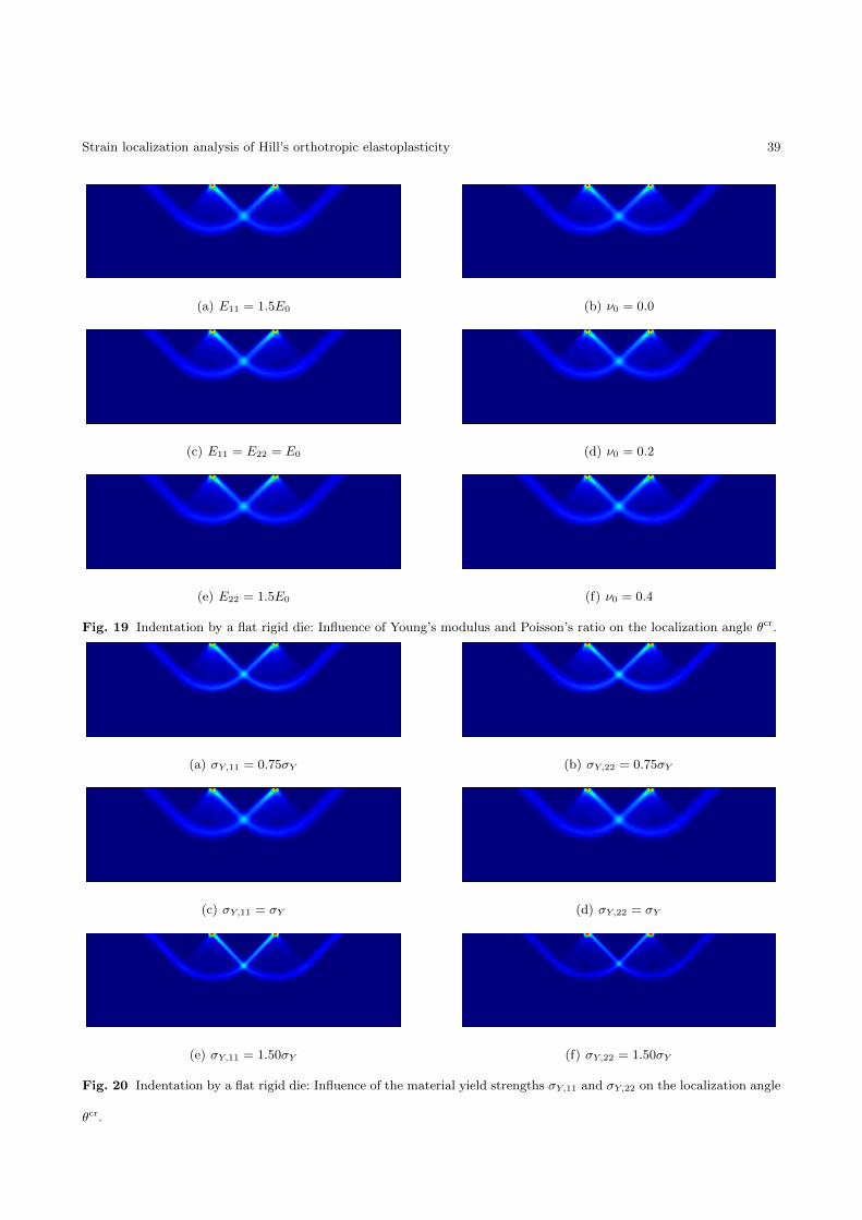
Strain localization analysis of Hill’s orthotropic elastoplasticity 39
(a) E11 = 1.5E0 (b) ν0 = 0.0
(c) E11 = E22 = E0 (d) ν0 = 0.2
(e) E22 = 1.5E0 (f) ν0 = 0.4
Fig. 19 Indentation by a flat rigid die: Influence of Young’s modulus and Poisson’s ratio on the localization angle θcr.
(a) σY,11 = 0.75σY (b) σY,22 = 0.75σY
(c) σY,11 = σY (d) σY,22 = σY
(e) σY,11 = 1.50σY (f) σY,22 = 1.50σY
Fig. 20 Indentation by a flat rigid die: Influence of the material yield strengths σY,11 and σY,22 on the localization angle
θcr.

40 Miguel Cervera et al.
(a) α = 0 (b) α = 30
(c) α = 45 (d) α = 60
Fig. 21 Indentation by a flat rigid die: Influence of the material yield strengths σY,11 = 1.5σY or σY,22 = 1.5σY on the
localization angle θcr.
(a) α = 0 (b) α = 30
(c) α = 45 (d) α = 60
Fig. 22 Indentation by a flat rigid die: Influence of the material yield strengths σY,11 = 0.75σY and σY,22 = 0.75σY on
the localization angle θcr.
View publication statsView publication stats