University of Calgary

PRISM: University of Calgary's Digital Repository

Haskayne School of Business Haskayne School of Business Research & Publications

2017

Store Incentives and Retailer Inventory Performance

under Asymmetric Demand Information and

Unobservable Lost Sales*

Alp, Osman; Sen, Alper

Alp, O. and Sen. A. (2017). Store Incentives and Retailer Inventory Performance under

Asymmetric Demand Information and Unobservable Lost Sales. Working Paper.

http://hdl.handle.net/1880/51883

journal article

Downloaded from PRISM: https://prism.ucalgary.ca

Store Incentives and Retailer Inventory Performanceunder Asymmetric Demand Information and

Unobservable Lost Sales*Osman Alp

Haskayne School of Business, University of Calgary, Calgary, AB, Canada osman.alp@ucalgary.ca

Alper SenDepartment of Industrial Engineering, Bilkent University Bilkent, Ankara, 06800, Turkey alpersen@bilkent.edu.tr

We study incentive issues in an inventory management setting in which high on-shelf availability is crucial.

Headquarters of a retailer delegates inventory replenishment decisions to store managers in its various stores.

Store manager has complete information of the local demand process, whereas headquarters has partial

information and cannot observe unsatisfied demand. The problem is how to incentivize the manager to make

an order quantity decision that minimizes the sum of headquarters’ expected overage and underage costs.

We propose two incentive schemes that explicitly incorporate excess inventory and stock-outs into the store

manager’s performance measurement. We prove that a perfect alignment of incentives is possible under certain

conditions. Interestingly, perfect or near-perfect alignment requires the stock-out inspection before the end of

the replenishment cycle. We validate our approach and assumptions on a retailer’s actual data and show that

the retailer may improve its profitability by using the proposed incentive scheme.

Key words : Incentive alignment, asymmetric information, unobservable shortages

1. Introduction and Literature Review

In this paper, we study incentive issues in an inventory management setting in which attaining

high on-shelf availability is crucial. In many industries, ramifications of stock unavailability can

be very costly. For example, for fast-moving consumer goods, the retail stock-out rates are around

8% in developed countries world-wide (Gruen et al., 2002) and have not changed much in the

past fifty years despite advances in information technology (Peckham, 1963, Coca-Cola Research

* Working Paper. Please do not cite or distribute without permission of the authors.

1

2

Council, 1996). Gruen et al. (2002) estimate that on the average 30% of items that are out of stock

are purchased from another store, costing retailers 4% of their sales annually. The authors also

estimate that 72% of the stock-outs were caused by retail store practices as opposed to problems

in the upstream of the supply chain. Nearly two-thirds of the store related stock-outs can be

attributed to store ordering and forecasting (47% of all stock-outs) which results in not having the

product anywhere in the store. The remaining one-third (25% of all stock-outs) can be attributed

to store shelving which leads to having the product in the store warehouse but not on the shelf.

A key factor for the severity of the stock-out problem in many retail environments is the

relative observability of obsolescence and stock-outs. When there is excess inventory that leads

to shrinkage or needs to be salvaged in a secondary market, this is an easily observable and

important event, whereas stock-outs are usually not easily observable and their adverse effects on

immediate and future revenues are not well-understood (Anderson et al., 2006). Therefore, a core

requirement to reduce stock-outs at the retailers is to develop an effective measurement system

(Gruen and Corsten, 2008), quantify the effect of stock-outs on profitability, and bring the issue to

the attention of the management (ECR Europe, 2003).

Given a large number of stores a typical retail chain owns, directly managing operations in

each store by headquarters is difficult. Hence, it is imperative “to design appropriate incentives

to motivate store managers to execute activities critical to the performance of the retail store”

(DeHoratius and Raman, 2007). These incentives, including those to reduce stock-outs and excess

inventory, can be tied to store managers’ performance scorecards. The balanced scorecard is a

common tool adopted for this purpose (Kaplan and Norton, 1992). Balanced scorecards may have

several perspectives, each having multiple objectives. For example, Tesco used a five segment

scorecard that includes customer, community, operations, people and finance-related dimensions

(Witcher and Chou, 2008). Stock-out related measures reside in the operations segment. Despite

the need for incentives, according to a survey by an alliance of food and consumer packaged goods

manufacturers and retailers, only nine percent of the retailers include stock-outs as a factor in their

3

incentives or rewards (FMI/GMA Trading Partner Alliance, 2015). Our communication with two

large grocery retail chains, a North American giant grocery retailer that owns several chain brands

and a European discount grocery chain, reveals that stock-outs are not explicitly contained in

their performance scorecards. These two retail firms utilize only two key performance indicators

(KPI) under the operations segment: “Sales Revenue” and “Inventory Shrinkage”. DeHoratius

and Raman (2007) also report that the same two KPIs are adopted by an American-based consumer

electronics retail store. When sales generation is based on self-service as in grocery retail stores,

on-shelf availability is one of the few factors that store managers can use to influence sales

(DeHoratius and Raman, 2007). Hence, lowering stock-outs is only implicitly accounted for in the

“Sales Revenue” KPI; lack of an explicit measure may not guarantee attaining the service levels

desired by the headquarters.

There are two challenges with using incentives related to stock-outs in practice. First, measuring

stock-outs may be difficult, if not impossible. Suggested approaches for measurement may either

require substantial effort on behalf of retailers or lead to inaccurate predictions of lost sales (Gruen

and Corsten, 2008). Second, store employees who are more heavily incentivised on availability

explicitly or through sales performance implicitly may care less about inventories which are

obviously also costly for the retailer. This leads to an incentive misalignment problem (see van

Donselaar et al., 2010 for an example of store managers that are only rewarded for on-stock

availability, order more or earlier than necessary). One option is to make the ordering decisions

systematic and centralized through the use of a computer-aided ordering (CAO) system. For

example, Tesco moved the ownership of ordering decisions from store managers to the supply

chain director (Corsten and Gruen, 2004). However this leads to local information that is only

available to store managers such as local events, variations in local demand, adjustments for

spoilage or shrinkage not being used for these critical decisions. Therefore, many retailers that

use CAO systems end up allowing stores to override the CAO recommendations (FMI/GMA

Trading Partner Alliance, 2015). Both retailers that we had communication with also have CAO

4

systems, with override privileges granted to their store managers. Hence, incentive schemes are

still necessary in most retail settings when an information asymmetry exists between stores and

headquarters.

In this paper, we propose an incentive and measurement scheme that attempts to include stock-

outs in scorecards with an easy-to-implement measure and address information asymmetry issues

mentioned above. We assume that a “principal” (a retailer or a manufacturer) needs to satisfy

uncertain customer demand over a finite horizon. The principal incurs the typical underage and

overage costs: for every unit of demand that is not satisfied there is a shortage cost; any inventory

left over at the end of the horizon incurs a holding cost per unit. Replenishment can take place

only before the horizon and that decision is delegated to an agent (such as a store manager or

an inventory manager) who is better informed about the demand process. The principal can

observe the inventory and sales throughout the horizon, but cannot observe unsatisfied demand.

Therefore, an incentive scheme based on the amount of shortages (such as penalizing the agent for

underage and overage in the same proportion of the principal’s underage and overage costs) is not

possible. The challenge for the principal is to design an incentive mechanism that induces the agent

to make an ordering decision that minimizes the principal’s expected overage and underage costs

under unobservable shortages and incomplete demand information. We suggest to incorporate

two measures into the store manager’s scorecard: A lump-sum penalty if a stock-out is observed

at a pre-specified instant in the horizon and a penalty proportional to the remaining stock at the

end of the horizon, both to be deducted from the performance score of the store manager.

We study the case where the underlying demand process is a Wiener Process, and the principal

only knows that the process is one of a finite number of such processes. We show that when

the possible Wiener Processes share the same variance, it is possible to induce the agent to order

the optimal quantity without revealing the exact demand information to the principal when the

stock-out measure is enforced based on the inventory level at the end-of-the horizon. What is

even more interesting is that checking and penalizing the stock-outs at an optimal time inside the

5

horizon (i.e., an “early inspection” scheme), rather than at the end, leads to perfect or near-perfect

alignment in more general cases. In particular, we show that the early inspection scheme can lead

to a performance that is strictly better than penalizing the stock-outs only at the end of horizon.

Our results also show that the proposed incentive schemes can be substantially more effective

than policies in which the principal does not delegate the replenishment decision to the store or

inventory manager, but instead relies on a CAO system.

The problem and our models are partially motivated by our interactions with a major European

discount grocer with over 1000 stores. The company competes on low prices as well as high

quality, which is ensured by a considerable weight of private label merchandise in its assortment

that consists of approximately 1000 SKUs. Products are shipped to stores on a weekly schedule

(certain products once a week, the others two or three times a week) from the company-owned

distribution centers using the company’s own fleet of trucks. The company uses a centralized CAO

system to create replenishment orders for its stores. The store managers have limited authority to

override the system. Actual order quantity recommendations of the system can be changed for

only a fixed percentage of the SKUs. In addition, the store manager may include more SKUs in the

replenishment, but the number of such new orders cannot exceed a certain percentage of SKUs

that are already in the replenishment. The company pulls data from its ERP system and reports the

number of SKUs without stocks at its stores and distribution centers to its senior management at

the end of each day. This is used to estimate the stock-outs and lost sales at the store level and root

causes are sought if the levels are unexpectedly high in a given day. The company acknowledges

the fact that store employees may have local information that could lead to improved forecasts and

replenishment, and perhaps to improved stock availability, but is unwilling to completely delegate

the replenishment decision to its store employees. There are several reasons. First, as mentioned

before, quantifying stock-outs and their effect on lost sales is difficult. Consequently, it is difficult

to devise an incentive mechanism that specifically builds on the trade-off between shortage and

inventory carrying costs. The company can only indirectly consider these in its current incentives;

6

store employees are rewarded for the sales and inventory shrinkage (loss of inventory due to

spoilage, theft, shoplifting, etc.) below a specific target. Finally, the company perceives that stock-

outs in its stores are not primarily due to store operations and they should focus more on problems

at its distribution center operations, logistics and procurement. In Section 3.4, we performed an

initial analysis for a limited number SKUs and store locations at this grocer. Our experiments with

actual demand data show that the retailer may improve its profitability considerably by using the

incentive schemes suggested in this paper. We do not have any data from the North American

chain to validate our approach. However, the performance measurement and the oversight of

store managers at this chain are similar, except that there are no restrictions on the override of

CAO recommendations.

While this incentive problem is very relevant for many industries with products that are replen-

ished periodically (such as fast-moving consumer goods, food and beverages, etc.), an alternative

motivation comes from another application we faced in the banking industry. The headquarters of

a bank delegates the nightly cash-loading decisions at its vast number of ATMs to local branches

which are believed to have more information about the cash demand in their localities (at least

more than what the headquarters may possess or can process). Excess cash carried in the ATMs is

obviously costly due to possible interest charges. Unsatisfied cash withdrawals are also costly due

to loss of goodwill. In addition, a good portion of withdrawals may lead to additional revenue

for the bank due to withdrawal fees or interests charged to credit cards. However, all these costs

or penalties are primarily borne by the headquarters. Since an ATM also serves the customers of

different branches or different banks, the local branch may not directly associate the service level

at the ATM to its own profitability or customer satisfaction. To prevent further customer dissat-

isfaction, ATMs usually warn the customers in case of a cash stock-out. Therefore, unsatisfied

cash withdrawal requests are not observable. The problem for the headquarters is to design an

incentive scheme for the branch managers such that they replenish ATMs with the amount of cash

that minimizes the headquarters’ expected inventory holding and shortage costs.

7

This paper is related to the literature on incentive alignment problems in supply chains. These

problems arise mainly due to hidden actions by the players in the chain, information asymmetries

or badly designed incentive schemes (Narayanan and Raman, 2004). Incentive problems are

relevant even for vertically integrated firms, as decisions at different echelons are often delegated

to individuals whose performance measurement schemes are not well aligned with the overall

profitability of the firm (Lee and Whang, 1999). Aligning or redesigning incentive schemes may

yield significant increases in profitability of the supply chain whether it is within the boundaries

of a single firm or consists of multiple independent firms. See Chen (2001) for a general review

of the earlier literature in this area. Information asymmetry can exist for cost parameters and/or

demand process. Asymmetric demand information is frequently observed in practice as the party

closer to the customer will have more information about localities and past sales (Khanjari et al.,

2014). Recent examples of asymmetric demand information considered in a supply chain context

include papers by Babich et al. (2012), Akan et al. (2012), and Dai and Jerath (2013). Similar to

our approach, these papers assume a finite set of states where each state has a corresponding and

known demand distribution. One of the supply chain parties exactly knows the state, whereas

the other party has a probabilistic knowledge. A related stream of literature is on accounting-

based performance measures that lead to effective delegation or goal-congruent performance

measures (e.g., Baldenius and Reichelstein, 2005). However, the emphasis of this literature on

inventory management is cases where a product is manufactured and sold in different periods.

In our setting, we assume a single period and focus on delegation of inventory decisions under

demand uncertainty. We also note that there are studies on designing incentive contracts for store

employees in retail settings (e.g., DeHoratius and Raman, 2007). However the focus in this strand

of literature is usually on aligning incentives when the store employees need to allocate effort

between multiple tasks.

Our paper is also related to the principal-agent problem which is a well-investigated topic in

economics literature (see Laffont and Martimort, 2009, for a comprehensive review of this problem).

8

In its most general form, a principal delegates a certain task to an agent through a contract which

induces the agent to act in alignment with the principal’s objective. Van Ackere (1993) and Schenk-

Mathes (1995) analyze this problem from an operations management perspective. In particular,

the agent is the more informed salesperson who decides how much effort to exert to generate

and flourish the demand, and the principal offers a corresponding incentive scheme (such as a

sales target and bonus). Zhang and Zenios (2008) extend the basic model to multiple periods and

dynamic information structures. Different from these studies, our focus is not the sales effort; we

assume that the agent’s (the store manager or the inventory manager) effort is fixed. Chu and Lai

(2013), Chen (2000), and Dai and Jerath (2013) extend the basic principal-agent model to include

inventory replenishment decisions which we also consider. However, unlike our setting, these

studies assume that the inventory replenishment decisions are made by the principal, and exploit

the interaction between product availability and the effort spent by the agent.

The incentive mechanism that we consider involves a fixed-penalty score deduction for stock-

outs. Inventory management under lump-sum penalty costs for shortages has been studied before

in the inventory literature, see, for example, papers by Bell and Noori (1984), Aneja and Noori

(1987), Cetinkaya and Parlar (1989), and Benkherouf and Sethi (2010). In fact, the first two papers

were also inspired by the examples from the banking industry which also partially motivated

us for this study. Our models extend the models in this stream to inventory management under

unobservable shortages and information asymmetry. Sieke et al. (2012) provide some examples

from different industries where fixed-penalty costs are charged when a party cannot satisfy a preset

service level. In particular, the authors consider the design problem of a “flat penalty contract”

in which the supplier is penalized if she cannot satisfy a percentage of the orders placed by a

manufacturer. They do not consider information asymmetry. Geng and Minutolo (2010) consider

a similar problem under information asymmetry. The retailer allocates space for a manufacturer’s

product in return for a fixed slotting (or failure) fee. The retailer (which is the more powerful party

in the chain) designs a contract which specifies a target sales volume and a failure fee which is

9

charged to the manufacturer if the sales target cannot be met at the end of the planning horizon.

The retailer also sets the ordering quantity and the sales price. Our problem setting is different as

the owner of the product is the more powerful party and has no control over the demand.

In this paper, we make the following contributions:

• We propose easy-to-implement performance measurement schemes to align the incentives of

store managers of multi-store retailers to those of their headquarters in settings where sales are

heavily driven by on-shelf availability. These schemes utilize a lump-sum penalty for a stock-out

occasion and a linear penalty for holding excess stock. Adopting such schemes may help retailers

reduce stock-outs and attain desired service levels across their stores.

• Under demand information asymmetry and certain conditions, we show that these schemes

lead to perfect incentive alignment.

• We show that “early inspection” schemes in which stock-outs are checked before the end

of the horizon, may lead to better alignment than checking for stock-outs only at the end of the

horizon. Early inspection unveils the severity of the lost demand with elevated precision, and this

leads to better alignment.

• Under more general settings, we show through numerical studies that these schemes lead to

near-perfect alignment of incentives.

• Even though our modeling approach predicates on a single item analysis, we propose an

easy-to-implement heuristic method that extends the schemes we suggest to handle multiple

items simultaneously. We show through numerical experiments that this method has an excellent

performance.

• By using the historical sales data of a retail chain, we show that these schemes can be used in

practice and lead to considerable revenue improvements.

The rest of the paper is organized as follows. In Section 2, we introduce the proposed incentive

schemes and analyze them under complete and incomplete information. We propose two incentive

schemes and show conditions where perfect alignment is possible. In Section 3, we conduct a

numerical study to quantify the benefits of the proposed incentive mechanisms. We conclude the

paper in Section 4.

10

2. Analysis of Alternative Incentive Schemes for Measuring InventoryManagement Performance

We consider a single item which is subject to stochastic demand and offered to the market through

several stores or sales channels. The principal, the owner or the main stakeholder of the item, hires

agents (e.g., store or inventory managers) who are in charge of inventory replenishment decisions

and sales operations. The stores could be different in size, located at distant regions, or have

structurally different demand patterns. The agents are able to observe full demand information

– the realized and lost demand – at their store, and have the most complete information for

forecasting their future demand. We assume that the item observes exogenous demand, indicating

that the sales effort exerted by the agents is fixed or does not influence the demand.

In this section, we propose and analyze alternative schemes used to evaluate the inventory

management performance of the agents. These schemes will aid the principal, albeit having

incomplete demand information, to incentivize the agents to make decisions in alignment with

her objective. In the following analysis, we focus on the principal’s interaction with one agent

only. This analysis can be replicated for all other agents since their operations are independent

from each other.

The planning horizon is finite with length T. The agent makes a single replenishment decision at

t = 0, the start of the planning horizon. The item observes stochastic demand on a continuous basis

until t = T, the end of the horizon. We assume that the accumulated demand at time t, X(t), follows

a Wiener Process with drift µ and variance σ2 throughout the horizon. By definition of the Wiener

Process, X(0) = 0 and the joint distribution of X(t0),X(t1), ...,X(tn) when tn > tn−1 > · · · > t1 > t0 > 0

satisfies the following conditions:

1. The differences X(tk) − X(tk−1) (total demand observed between tk−1 and tk) are mutually

independent normal distributed random variables.

2. The mean of the difference X(tk)−X(tk−1) = (tk − tk−1)µ.

3. VAR [X(tk)−X(tk−1)] = (tk − tk−1)σ2.

11

Wiener Process or Brownian motion is frequently used in the inventory literature (e.g., Rudi et al.,

2009, Rao, 2003). In order to ensure that the probability of negative demand is negligibly small, one

can assume that the drift µ is sufficiently larger than variance σ (e.g., µ > 3.5σ). By definition, the

demand observed throughout the horizon, denoted by D, follows Normal distribution with mean

Tµ and variance Tσ2. The agent knows the exact values of these parameters whereas the principal

has partial information. In particular, we assume that the principal knows that the demand is

governed by one of N possible Wiener Processes with a parameter pair (µi, σi) with probability λi

for i = 1, ...,N where∑N

i=1λi = 1.

The principal incurs an overage cost, co, for each unit of excess inventory and an underage cost,

cu, for each unit of unmet demand at the end of the horizon at each of the stores. The excess

inventory or an out-of-stock situation at the stores can easily be tracked by both the principal

and the agent with an information system, however, the principal cannot observe the quantity

of the lost demand, if any. Moreover, the principal has incomplete information of the demand

distribution. Consequently, the principal cannot determine the optimal replenishment quantity

that minimizes her expected total overage and underage cost. As a remedy to this, we devise

two incentive schemes that will be imposed on the agent based on his inventory replenishment

decisions. It is assumed that the agent will take the optimal course of action which maximizes his

performance (equivalent to minimizing the his performance score in the imposed scheme). The

principal will utilize this to incentivize the agent to take actions in favor of her objective.

We propose two incentive schemes, [M] and [M, t], each of which contains two key performance

indicators: excess inventory and shortage. Let It be the on-hand inventory at time t and 1{It=0} be an

indicator function which is equal to 1 if It = 0, and 0 otherwise. The performance score of scheme

[M] is calculated by

PS[M] = co × IT + M× 1{IT=0}

where co and M are the parameters to be set by the principal. Similarly, the performance score of

the scheme [M, t] is calculated by

PS[Mt] = co × IT + M× 1{It=0}

12

where co, M, and t are the parameters to be set by the principal. Since both excess inventory and

inventory shortage are costly for the principal, the lower values of the scores in these schemes

indicate a better performance for the agent.

The agent decides on the number of items to order, denoted by Qa, at the beginning of each

planning horizon in a way that minimizes his performance score. Predicating on the prospective

decision of the agent, the principal has the liberty to set the values of co, M, and/or t, so that the Qa

value chosen by the agent is close to the order quantity that minimizes the principal’s expected

total overage and underage cost.

2.1. Scheme [M]

In this section, we analyze scheme [M] from the principal’s and agent’s perspectives.

2.1.1. Agent’s Problem Under scheme [M], the expected performance score of the agent is

given by the following expression:

EPS[M](Qa) = coE[max{Qa −D,0}] + MP{D≥Qa}=

∫ Qa

−∞

c0(Qa − x) f (x)dx +

∫∞

Qa

M f (x)dx

where f is the probability density function (pdf) of D, the total demand observed during the

planning horizon. For the case of Wiener Process with parameters µ and σ, f is the density of a

Normal random variable with mean Tµ and standard deviation√

Tσ. We assume that the agent

has complete demand information, i.e., these parameters are known by the agent.

We first provide a theorem which shows that the optimal order quantity that maximizes

agent’s performance is a function of the reversed hazard rate function of the demand distribution.

Reversed hazard rate is defined by f (x)F(x) for any random variable with pdf, f (x), and cumulative

distribution function (cdf), F(x). Marshall and Olkin (2007) show that this function is decreasing if

the random variable has log-concave density. Many densities including uniform and Normal are

log-concave (Bagnoli and Bergstrom, 2005).

Theorem 1 The optimal order quantity of the agent that maximizes his performance under scheme [M] is

given by Q∗a = r−1(

Mco

)where r(x) = F(x)

f (x) is the reciprocal of the reversed hazard rate function of the demand

distribution.

13

Proof: The first order condition of the function EPS[M](Qa) yields the following equality.

F(Q∗a)f (Q∗a)

=Mco.

Since, the reversed hazard rate is a decreasing function when the demand is Normal (because of

its log-concavity), r(Q∗a) =F(Q∗a)f (Q∗a) is an increasing function and hence, EPS[M](Qa) is quasi–convex and

its unique extremum is a minimum. �

If the principal uses scheme [M] with parameters co and M as the performance measure of the

agent and knows the demand distribution with certainty, then she can anticipate that the agent

will order r−1(

Mco

)units for each planning horizon.

2.1.2. Principal’s Problem under Complete Information Suppose that there is no information

asymmetry between the agent and the principal. This implies that N = 1 and λ1 = 1. Principal’s

objective function can be stated as:

ETC(Qp) = coE[max{Qp −D,0}+ cuE[max{D−Qp,0}]

where Qp is the replenishment quantity. This is the well-studied Newsvendor problem and it is

well-known that Q∗p = F−1(α) minimizes the above function where α = cucu+co

. The principal wants

the agent to order Qa = Q∗p. The principal can achieve this by anticipating the optimal action of

the principal stated in Theorem 1 and imposing the incentive scheme [M] with the values of the

parameters co and M that satisfy

Q∗a = Q∗p ⇒Mco

=F(Q∗a)f (Q∗a)

=F(Q∗p)

f (Q∗p)=

F(F−1(α))f (F−1(α))

=α

f (F−1(α)).

Since the parameters of the incentive scheme do not correspond to any financial value, co can

simply be set to 1 and the parameter M can be set to

M =α

f (F−1(α)).

The function s(τ) = 1f (F−1(τ)) is called the sparsity function by Tukey (1965) or the quantile density

function by Parzen (1979). The sparsity function for Normal density with µ and σ is given by

14

sN(τ) =√

2πσe(Φ−1(τ))2

2 where Φ is the cdf of the standard Normal random variable. Consequently,

a perfect alignment is possible under scheme [M] and complete information, when the principal

sets the parameters to co = 1 and M = αsN(α). We note that this quantity is independent of the mean

demand µ and is only a function of the standard deviation.

2.1.3. Principal’s Problem under Incomplete Information Under incomplete information, we

know by Theorem 1 that the agent orders

Qi = r−1i

(Mco

),

if the exact demand process is Di with parameters µi and σi. Then the corresponding cost incurred

for the principal is

ETCi(Qi) = coE[max{Qi −Di,0}+ cuE[max{Di −Qi,0}].

Since the exact demand distribution could be any of the N scenarios with probability λi, the

principal’s expected cost would beN∑

i=1

λi ·ETCi(Qi).

By presetting the parameter co = 1, the principal solves the following optimization problem

PPM(N) : MinN∑

i=1

λiETCi(Qi)

s.to Qi = r−1i (M) ∀i

to find the value for the parameter M that will incentivize the agent to order in a way that minimizes

the principal’s expected total cost under [M] scheme. In this problem, the decision variables are

Qi for i = 1, . . . ,N and M. This problem can be restated as an unconstrained optimization problem

with a single decision variable, M as

MinN∑

i=1

λiETCi(r−1i (M)). (1)

Clearly, the principal’s cost under incomplete information is higher than or equal to her cost

under complete information as a single M value may not lead the agent to order Q∗p in each

15

possible scenario. If this could be achieved, then a perfect alignment situation would be instated.

This ideal situation can be achieved only if r1(Q∗p) = r2(Q∗p) = · · · = rN(Q∗p). In such a case, setting

M = ri(Q∗p) = ri(F−1(α)

)for any demand scenario i would lead to perfect alignment. The following

theorem characterizes a situation where this is attainable.

Theorem 2 If the possible demand processes have the same standard deviation σ, then setting M∗ = αs(α)

leads the agent to select Q∗p in each possible demand scenario i.

Proof: If all distributions have the same σ, then ri(Q∗p) = αs(α) for all i as s(α) is only a function of

σ. �

Theorem 2 states that perfect alignment is possible under scheme [M] with a reasonable demand

scenario1. This scenario is observed when the variability of demand is exogenous to the factors

that differentiate alternative demand processes. In such cases, the differentiating factor will be the

expected value of demand. In all cases other than this scenario, perfect alignment is not possible.

For such cases, the following theorem provides a system of linear equations that solves Problem

(1).

Theorem 3 The following system of linear equations yields the optimal value of parameter M.N∑

i=1

λi(Φ(zi)−α)

1 + ziΦ(zi)φ(zi)

= 0 and σiΦ(zi) = Mφ(zi), i = 1, . . . ,n

Proof : Recall that the agent’s optimal ordering quantity satisfies r(Q) = F(Q)f (Q) = M. Since the demand

is Normal, this equation can be rewritten as r(z) = σΦ(z)φ(z) = M with Q = µ + zσ transformation.

Similarly, the expected total cost of the principal can be rewritten as follows (Porteus, 2002):

ETC(Q)≡ L(z) = σ(coz + (co + cu)

[φ(z)− z(1−Φ(z))

])= σ

((co + cu)zΦ(z) + (co + cu)φ(z)− cuz

).

1 Note that perfect alignment may be obtained for demand processes other than Wiener. For example, the sparsity

function for uniform distribution between a and b is given by s(τ) = b− a. Therefore, if the total demand is distributed

with one of a number of uniform distributions with same interval length, the principal can also incentivize the agent to

order its optimal quantity.

16

By using z = Φ−1(α), L(Φ−1(α)) = σ[(co + cu)Φ−1(α)α+ (co + cu)φ(Φ−1(α))− cuΦ

−1(α)]. Using α∗ =

cu/(co + cu) and multiplying this function with 1/(co + cu), we obtain L(Φ−1(α)) = 1co+cu

L(Φ−1(α)) =

σ[αiΦ

−1(αi) +φ(Φ−1(αi))−α∗Φ−1(αi)].

Using these expressions, (1) is equivalent to the following optimization problem:

minM

N∑i=1

λiL(r−1(M/σi))

where we redefine r(z) as Φ(z)φ(z) in the rest of this proof. Then, the first order condition is

N∑i=1

λiL′(r−1(M/σi))dr−1(M/σi)

dM= 0.

Since r(r−1(x)) = x, differentiating both sides, we get

r′(r−1(x))dr−1(x)

dx= 1.

But,

r′(z) =(φ(z))2

−φ′(z)Φ(z)(φ(z))2

=φ(z) + zΦ(z)

φ(z)= 1 + zr(z)⇒

dr−1(M/σi)dM

=(1/σi)

(1 + (M/σi)r(M/σi)).

Then the first order condition becomes

N∑i=1

λiσi(Φ(r−1(M/σi))−α∗)

σi(1 + r−1(M/σi)(M/σi))=

N∑i=1

λi(Φ(r−1(M/σi))−α∗)(1 + r−1(M/σi)(M/σi))

= 0.

We can also write this as a system of equations in zi and M to obtain the desired result.

N∑i=1

λi(Φ(zi)−α∗)

1 + ziΦ(zi)φ(zi)

= 0 and σiΦ(zi) = Mφ(zi) ∀i = 1, . . . ,N.

�

2.2. Scheme [M, t]

Scheme [M, t] is similar to scheme [M] with the difference that the M value is contributed to the

performance score if on-hand inventory at time t < T is equal to zero, rather than at t = T. The

scheme can be called as an “early inspection” scheme and builds on the fact that discovering

17

a stock-out earlier in the horizon may lead to a better understanding of the actual amount of

unsatisfied demand for the principal. Notice also that this scheme provides more information to

the principal since a stock-out at given time t < T also means a stock-out at time T, but not vice

versa. First, we analyze the agent’s problem in detail under this scheme, and then show that it

outperforms scheme [M] under certain conditions. Without loss of generality, we set T = 1 in the

following discussion.

2.2.1. Agent’s Problem Let Y and Y be the random variables denoting demand during [0, t]

and [t,1], respectively. Then, we have X(t) − X(0) = Y ∼ N(tµ,√

tσ) and X(1) − X(t) = Y ∼ N((1 −

t)µ,√

1− tσ) by the definition of Wiener Process. Let G (g) and H (h) denote the cdf (pdf) of the

random variables Y and Y, respectively. Then, the agent’s performance score for any realization

of y and y, and order quantity of Qa, is given by

PS[Mt](Qa) =

M if y≥Qa and y + y≥Qa

M + co(Qa − (y + y)) if y≥Qa and y + y≤Qa

0 if y≤Qa and y + y≥Qa

co(Qa − (y + y)) if y≤Qa and y + y≤Qa.

Then, the expected performance score for any order quantity Qa is given by

EPS[Mt](Qa) =

∫∞

Qa

∫∞

Qa−yMh(y)g(y)dydy + 0 + 0 +

∫ Qa

−∞

∫ Qa−y

−∞

coh(Qa − (y + y)

)h(y)g(y)dydy

=

∫∞

Qa

Mg(y)dy +

∫ Qa

−∞

∫ Qa−y

−∞

coh(Qa − (y + y))h(y)g(y)dydy

= M(1−G(Qa)) +

∫ Qa

−∞

∫ Qa−y

−∞

coh(Qa − (y + y))h(y)g(y)dydy.

A Wiener Process, W(µ,σ2; t), has the following Markovian property (see Patel and Read, 1982):

Property 1 The W(µ,σ2; t) process has the Markov property that the conditional distribution of X(t)− a,

given that X(u) = a for t > u, is that of µ(t− u) + σZ√

t−u where Z is the standard Normal variate. This

distribution is independent of the history of the process up to time u.

18

Property 1 implies that the total demand observed during the planning horizon, Y + Y, is

independent of any particular realization of Y. Consequently, the agent’s expected cost function

can be re-written as

EPS[Mt](Qa) = MP{Y ≥Qa}+ coE[max{Qa −D},0] = M∫∞

Qa

g(x)dx + co

∫ Qa

−∞

(Qa − x) f (x)dx.

By letting co = 1, z =Qa−µ

σ , zt =Qa−tµ√

tσ, k =

µ

σ , a = k(1− t), and noting that zt = a+z√

t, we have

EPS′[Mt](Qa) = F(Qa)−Mg(Qa)≡ω(z) = Φ(z)−M√

tσφ

(a + z√

t

), (2)

EPS′′[Mt](Qa) = f (Qa)−Mg′(Qa) =ω′(z)≡ δ(z) =φ(z) +M(a + z)

t√

tσφ

(a + z√

t

). (3)

Lemma 1 If M > e−12 (k2(1−t)) √tσ

k then ω(z) has only one local finite minimum. Otherwise, ω(−k) ≤ ω(z) for

all z≥−k.

Proof: First we show that the local optima of ω(z) for z≥−k are finite.

limz→−k

ω(z) = Φ(−k)−M√

tσφ

(k(1− t)− k√

t

)= Φ(−k)−

Mφ(−k)√

tσ.

limz→∞

ω(z) = Φ(∞)−M√

tσφ

(k(1− t) +∞√

t

)= 1− 0 = 1.

Moreover, ω(z) is a continuous function for all z : z ∈ [−k,∞). Hence, all local optima of ω(z) must

be finite. Next, we show that there can be at most one local optimum of ω(z). We show this by

showing that there can be at most one z that satisfies ω′(z) = δ(z) = 0. Equating (3) to 0, we get

φ(z) =−M(a + z)

t√

tσφ

(a + z√

t

),or

φ(z)

φ(

a+z√

t

) +Mz

t√

tσ=−Ma

t√

tσ,or

e−

12

(z2−

(a+z)2t

)+

Mz

t√

tσ=−Ma

t√

tσ. (4)

Denote the left-hand side of (4) by d(z). Next, we show that d(z) is an increasing function. One can

show that

d′(z) =−12

(2z−

2(a + z)t

)e−

12

(z2−

(a+z)2t

)+

M

t√

tσ≥ 0,

19

since a ≥ 0, t ≤ 1, and 2z ≤ 2zt . Therefore, (4) can hold only for one value of z since its right-hand

side is a constant. Consequently, if d(−k) > −Mat√

tσthen δ(z) , 0 for all z ≥ −k and w(z) has one local

minimum. Since

d(−k) = e−

12

(k2−

(k(1−t)−k)2t

)−

Mk

t√

tσ,

d(−k)> −Mat√

tσis equivalent to the condition

e− 12 (k2(1−t))

√tσ

k< M. �

We are now ready to present the main result of this section. The following theorem characterizes

the optimal ordering quantities of the agent under different parameter ranges.

Theorem 4 The optimal order quantity is characterized by the following rules:

1. If M> Φ(−k)φ(−k

√t)

√tσ then z∗ :ω(z∗) = 0 is unique and corresponds to the optimal order quantity.

2. If M< Φ(−k)φ(−k

√t)

√tσ and M< e−

12 (k2(1−t)) √tσ

k then z∗ =−k.

3. If e−12 (k2(1−t)) √tσ

k <M< Φ(−k)φ(−k

√t)

√tσ then there exist at most two values of z such that ω(z) = 0. Either one

of these two z values or z =−k correspond to the optimal order quantity.

Proof: First note that, limz→−kω(z) = Φ(−k) − M√

tσφ

(k(1−t)−k√

t

)= Φ(−k) − M

√tσφ(−k

√t). So, ω(−k) < 0 if

M> Φ(−k)φ(−k

√t)

√tσ and ω(−k)> 0 otherwise.

(1) Under this condition ω(−k) < 0. In this case, ω(z) = 0 can hold only once for some z ≥ −k

because of Lemma 1.

(2) Under this condition ω(−k) > 0. When ω(−k) is positive and when M < e−12 (k2(1−t)) √tσ

k , ω(−k)

cannot have any local minimum due to Lemma 1, and hence ω(z) > 0 for all z ≥ −k. Therefore,

z∗ =−k must correspond to the optimal order quantity.

(3) Under this condition ω(−k)> 0. When M> e−12 (k2(1−t)) √tσ

k , ω(z) has one local optimum at which

either ω(z)> 0 or ω(z)< 0. If ω(z)> 0, then ω(z) can never attain a value of 0 so z∗ =−k corresponds

to the optimal order quantity. If ω(z)< 0 then ω(z) must attain the value of zero twice so one of the

z values that satisfy ω(z) = 0 must correspond to the optimal order quantity. �

20

2.2.2. Principal’s Problem under Incomplete Information In this part, we assume that M >

Φ(−k)φ(−k

√t)

√tσ under which the optimal order quantity of the agent is the unique value that satisfies

the first order condition (Theorem 4.1). From (2), the optimal order quantity of the agent satisfies

the following equality when the agent’s demand distribution assumes the ith parameters:

Φ(zi)

φ(

ki(1−t)+zi√

t

) √tσi = M

where ki =µiσi

. Then, the principal solves the following problem:

PPMt(N) : MinM,t,zi

N∑i=1

λiLi(zi)

s.to qi(zi, t) = M ∀i = 1, ...,N

where Li(zi) = coziσi + (co + cu)σi

[φ(zi)− zi(1−Φ(zi))

]and qi(zi, t) =

Φ(zi)

φ(

ki(1−t)+zi√t

) √tσi. Note that Li(zi) ≡

ETCi(Qi) when Qi = µi + ziσi.

The principal prefers the agent to calculate z∗i = Φ−1(

cuco+cu

)= z and set his order quantity as

Qi = µi + zσi. This will lead to perfect alignment. The following result shows that this is achievable

when N = 2 under a mild condition.

Theorem 5 When N = 2, if k2 > k1, and σ2 < σ1, then there exists a τ such that 0< τ < 1 which satisfies

e−

12

[(k2(1−τ)+z)2−(k1(1−τ)+z)2

τ

]=σ2

σ1.

The scheme [M, t] with parameters co = 1, t = τ, and M = Φ(z)

φ(

k1(1−τ)+z√τ

) √τσ1 = Φ(z)

φ(

k2(1−τ)+z√τ

) √τσ2 incentivizes

the agent to order an amount that corresponds to z, which is equal to the optimal order quantity for the

principal.

Proof: PPMt(2) can be written as:

Mint,z1,z2

2∑i=1

λiLi(zi)

s.to q1(z1, t) = q2(z2, t)

Given the values of M and t, we know that agent will pick a z value that satisfies q1(z1, t) = M or

q2(z2, t) = M depending on whether the exact demand distribution is f1 or f2. We also know that

21

z1 = z2 = z is the ideal operating point of the principal. Hence, the question is whether there is a τ

value that is feasible for PPMt(2) where z1 = z2 = z? For feasibility, we must have q1(z, τ) = q2(z, τ).

This is equivalent to:

Φ(z)

φ(

k1(1−τ)+z√τ

) √τσ1 =Φ(z)

φ(

k2(1−τ)+z√τ

) √τσ2,or

φ(

k2(1−τ)+z√τ

)φ

(k1(1−τ)+z√τ

) =σ2

σ1,or

e−

12

[(k2(1−τ)+z)2−(k1(1−τ)+z)2

τ

]=σ2

σ1. (5)

Denote the left-hand side of (5) as l(τ). Note that limt→0 l(t) = 0, limt→1 l(t) = 1 and the function l(t)

is continuous on (0,1]. Hence, Equation (5) must be satisfied at some τ ∈ (0,1) since 0< σ2σ1< 1. �

Note that the condition of Theorem 5 is also satisfied when µ1 = µ2 and σ1 > σ2. This result has

two implications. First, it is possible to incentivize the agent to order a quantity which is equal

to the optimal order quantity of the principal under incomplete information. Second, the scheme

[M, t] outperforms scheme [M] under certain parameter ranges. Next, we generalize the latter

result for N > 2.

Lemma 2 If σ1 ≥ σ2 ≥ · · · ≥ σN−1 ≥ σN, then z∗1 ≤ z∗2 ≤ · · · ≤ z∗N−1 ≤ z∗N and z∗1 ≤ z ≤ z∗N in the optimal

solution of PPM(N) where z = Φ−1(α).

Proof : PPM(N) can be stated as

Min z1,...,zN

N∑i=1

λiLi(zi)

s.toΦ(zi)φ(zi)

σi =Φ(zi+1)φ(zi+1)

σi+1 ∀i = 1, . . . ,N− 1.

Since Φ(z)φ(z) is monotonically increasing function and σi ≥ σi+1, the ith constraint can be satisfied

only if z∗i ≤ z∗i+1 for all i = 1, . . . ,N− 1. This proves the first inequality.

Case 1. z∗1 ≤ · · · ≤ z∗N < z.

Let z′1 be such that Φ(z)φ(z)σN =

Φ(z′1)

φ(z′1)σ1. Since Φ(z)φ(z) is increasing in z and σ1 ≥ σN, we have z′1 ≤ z.

Moreover, since z∗N ≤ z, we haveΦ(z∗N)

φ(z∗N) ≤Φ(z)φ(z) . Noting that z∗1 and z∗N satisfy the constraints of PPM(N),

we can write

22

Φ(z∗1)φ(z∗1)

σ1 =Φ(z∗N)φ(z∗N)

σN <Φ(z)φ(z)

σN =Φ(z′1)φ(z′1)

σ1.

⇒Φ(z∗1)φ(z∗1)

σ1 <Φ(z′1)φ(z′1)

σ1⇒ z∗1 < z′1 < z⇒ L1(z∗1)> L1(z′1).

Let z′2, z′

3, . . . , z′

N−1 be such thatΦ(z′1)

φ(z′1)σ1 =Φ(z′i )

φ(z′i )σi for all i = 2, . . . ,N − 1. SinceΦ(z∗1)

φ(z∗1)σ1 =Φ(z∗i )

φ(z∗i )σi for i =

2, . . . ,N− 1 and z∗1 < z′1, we must have z∗i < z′i and Li(z∗i )> L(z′i ) for all i = 2, . . . ,N− 1. Last inequality

is due to convexity of function L. Hence,

λ1L1(z∗1)+λ2L2(z∗2)+ · · ·+λN−1LN−1(z∗N−1)+λNLN(z∗N)≥ λ1L1(z′1)+λ2L2(z′2)+ · · ·+λN−1LN−1(z′N−1)+λNLN(z).

Last inequality violates the optimality of 〈z∗1, z∗

2, . . . , z∗

N−1, z∗

N〉 as 〈z′1, z′

2, . . . , z′

N−1, z〉 is also feasible to

PPM(N) and produces a lower cost. Hence, z∗N � z.

Case 2. z< z∗1 ≤ · · · ≤ z∗N.

This case can be proven with similar arguments of Case 1. �

Theorem 6 If k1 ≤ k2 ≤ · · · ≤ kN and σ1 ≥ σ2 ≥ · · · ≥ σN, then there exists a scheme [M, t] with t < 1 which

outperforms scheme [M].

Proof: Suppose that < z∗1, z∗

2, . . . , z∗

N > is an optimal solution to PP(N). Due to Lemma 2, we have

z∗1 ≤ z∗2 ≤ · · · ≤ z∗N.

We can rewrite PPMt(N) as

Mint,z1,z2,...,zN f (z1, z2, . . . , zN, t)

s.to gi(z1, z2, . . . , zN, t) = 0 ∀i = {1,2, . . . ,N− 1}

where

f (z1, z2, . . . , zN, t) = λ1L1(z1) +λ2L2(z2) + · · ·+λNLN(zN),

g1(z1, z2, . . . , zN, t) = q1(z1, t)− q2(z2, t),

g2(z1, z2, . . . , zN, t) = q1(z1, t)− q3(z3, t),

...

gN−1(z1, z2, . . . , zN, t) = q1(z1, t)− qN(zN, t).

23

Note that x0 = 〈z∗1, z∗

2, . . . , z∗

N,1〉 is also a feasible solution to PPMt(N) and satisfyΦ(z∗1)

φ(z∗1)σ1 =Φ(z∗2)

φ(z∗2)σ2 =

Φ(z∗3)

φ(z∗3)σ3 = · · ·=Φ(z∗N)

φ(z∗N)σN = M for some value of M.

x0 can be an optimal solution only if it satisfies the KKT necessary conditions

∇ f (x0) + v1 · ∇g1(x0) + v2 · ∇g2(x0) + · · ·+ vN−1 · ∇gN−1(x0) =−→0 (6)

for some values of v1,v2, . . . ,vN−1. First we note that

∂q(z, t)∂t

=

12Φ(z)t−1/2σφ

(a+z√

t

)+ Φ(z)

√tσ a+z√

tφ

(a+z√

t

)−k√

t−(a+z) 12 t−1/2

t

φ2(

a+z√

t

)∂q(z, t)∂t

∣∣∣∣∣t=1

=Φ(z)φ(z)

σ[12− z

(k +

z2

)].

Further, we can write the following partial derivatives:

∂ f∂z1

(x0) = λ1L′1(z∗1),∂ f∂z2

(x0) = λ2L′2(z∗2), . . . ,∂ f∂zN

(x0) = λNL′N(z∗N),∂ f∂t

(x0) = 0,

∂g1

∂z1(x0) =

σ1(φ(z∗1) + z∗1Φ(z∗1))φ(z∗1)

= σ1 + z∗1M,

∂g1

∂z2(x0) =

−σ2(φ(z∗2) + z∗2Φ(z∗2))φ(z∗2)

=−(σ2 + z∗2M),

∂g1

∂z3(x0) = · · ·=

∂g1

∂zN(x0) = 0,

∂g1

∂t(x0) =

Φ(z∗1)σ1

φ(z∗1)

[12− z∗1

(k1 +

z∗12

)]−

Φ(z∗2)σ2

φ(z∗2)

[12− z∗2

(k2 +

z∗22

)]= Mz∗2

(k2 +

z∗22

)−Mz∗1

(k1 +

z∗12

),

∂g2

∂z1(x0) = σ1 + z∗1M,

∂g2

∂z2(x0) = 0,

∂g2

∂z3(x0) =−(σ3 + z∗3M),

∂g2

∂z4(x0) = · · ·=

∂g2

∂zN(x0) = 0,

∂g2

∂t(x0) =

Φ(z∗1)σ1

φ(z∗1)

[12− z∗1

(k1 +

z∗12

)]−

Φ(z∗3)σ3

φ(z∗3)

[12− z∗3

(k3 +

z∗32

)]= Mz∗3

(k3 +

z∗32

)−Mz∗1

(k1 +

z∗12

),

...

∂gN−1

∂z1(x0) = σ1 + z∗1M,

∂gN−1

∂z2(x0) = · · ·=

∂gN−1

∂zN−1(x0) = 0,

∂gN−1

∂zN(x0) =−(σN + z∗NM),

∂gN−1

∂t= Mz∗N

(kN +

z∗N2

)−Mz∗1

(k1 +

z∗12

).

We can rewrite (6) as follows:

λ1L′1(z∗1) + v1 · (σ1 + z∗1M) + v2(σ1 + z∗1M) + vN−1(σ1 + z∗1M) = 0

λ2L′2(z∗2)− v1(σ2 + z∗2M) = 0 (7)

24

λ3L′3(z∗3)− v2(σ3 + z∗3M) = 0 (8)

...

λNL′N(z∗N)− vN−1(σN + z∗NM) = 0 (9)

0 + v1M(z∗2

(k2 +

z∗22

)− z∗1

(k1 +

z∗12

))+ v2M

(z∗3

(k3 +

z∗32

)− z∗1

(k1 +

z∗12

))+ · · ·

+vN−1M(z∗N

(kN +

z∗N2

)− z∗1

(k1 +

z∗12

))= 0 (10)

From (7) - (9): vi =λi+1L

′

i+1(z∗i+1)

σi+1+z∗i+1M for i = 1, . . . ,N− 1. Plug v1,v2, . . . ,vN−1 into (10) to obtain

N−1∑i=1

λi+1L′i+1(z∗i+1)σi+1 + z∗i+1M

M[z∗i+1

(ki+1 +

z∗i+1

2

)− z∗1

(k1 +

z∗12

)]= 0

⇒

N−1∑i=1

λi+1L′i+1(z∗i+1)σi+1 + z∗i+1M

z∗i+1

(ki+1 +

z∗i+1

2

)=

N−1∑i=1

λi+1L′i+1(z∗i+1)σi+1 + z∗i+1M

z∗1

(k1 +

z∗12

)However, this last equality cannot hold because ki ≥ k1 and z∗i ≥ z∗1 for all i = 2, . . . ,N, and hence x0

cannot be an optimal solution. �

2.3. Computer Aided Ordering

As discussed in Section 1, many multi-store retailers have embedded CAO method in their order-

ing systems. This computerized method suggests the store manager an order quantity for each

item in the store, based on historical demand/sales data. The main pitfall is that the historical

data might include demand streams originating from distinct populations and the store managers

might have a better idea of the temporal realization of the streams. To remedy this pitfall, some

retailers let the store managers override the proposed quantities to a certain extent.

Let X denote the random variable corresponding to the aggregated demand observed by the

retailer. Then, along with the lines of our modeling approach, we have X =∑N

i=1λiXi. In this case,

the CAO system will propose an order quantity, Qp, which solves the following problem::

PPCAO : MinQp

N∑i=1

λi

co

∫ Qp

−∞

(Qp − x) fi(x)dx + cu

∫∞

Qp

(x−Qp) fi(x)dx

25

where fi is the pdf of the ith demand stream. The problem is equivalent to solving a Newsvendor

problem when the demand follows a mixture of N Normal random variables, with ith variable

having a meanµiT and standard deviation σi

√T. In Section 3, we show through numerical analysis

that a pure CAO system is inferior to our proposed incentive schemes.

3. Numerical Study

In this section, we present the results of a numerical study we conducted (i) to investigate the value

of the proposed schemes in aligning incentives of both parties and (ii) to identify the parameter

ranges for which these schemes bring a superior alignment. We experiment with two problem sets.

The first set contains demand streams with the same coefficient of variations and the other with

randomized parameters. In the first problem set, the number of possible demand distributions,

N, is set to 3 with drift parameters µ1 = 20, µ2 = 30, and µ3 = 40. The standard deviation of each

demand process is set to

σi = CoV ·µi ∀i = 1,2,3 with CoV ∈ {0.1,0.15,0.2,0.25}.

Note that CoV corresponds to the coefficient of variation of the demand process and is assumed to

be constant across all possible demand processes in a given problem instance. The overage cost,

co, is set to 1 and the underage cost, cu, takes one of the following values: {2,5,10,20}. Finally, the

weights of the potential demand processes are set to

λ1 ∈ {1/3,0.5,0.75,0.9}, λ2 = λ3 =1−λ1

2.

Note that as λ1 increases, the level of information asymmetry decreases. In total, we generate

4 × 4 × 4 = 64 different problem instances by enumerating all possible combinations of the four

different values for each of the parameters cu (overage cost), CoV (demand variation), and λ1 (level

of information asymmetry).

Let ETCPI denote the minimum expected total cost of the principal under perfect demand

information. This value is given by the unconstrained solution of problem PPM(N) and is the

26

principal’s minimum possible cost value. Let ETCM, ETCMt, and ETCCAO denote the optimal cost

obtained by solving PPM(N), PPMt(N), and PPCAO, respectively. We define IncM and IncMt to denote

the cost increment for schemes [M] and [M, t], respectively, relative to the ideal but hypothetical

case of perfect information. We define these measures as

IncM =ETCM −ETCPI

ETCPI,

IncMt =ETCMt −ETCPI

ETCPI.

Lower values of IncM and IncMt correspond to better alignment between the principal and the

agent. We quantify the potential savings obtained by the [M, t] scheme rather than relying on CAO

system by

SavCAO =ETCCAO −ETCMt

ETCCAO.

We conjecture that the delegation of inventory replenishment to an agent through [M, t] scheme

would outperform CAO system. In this case, SAVCAO returns a positive value.

3.1. Performances of [M] and [M, t] Incentive Schemes

Out of the 64 problem instances solved, the minimum, maximum, and average values of IncM

are 0.97%, 4.77%, and 2.26%, respectively. The same values for IncMt are 0.04%, 0.15%, and 0.09%,

respectively. These numbers reveal the strength of the scheme [M, t] for aligning incentives of

the agent and the principal. Table 1 depicts the average IncMt values for each combination of

(CoV, λ1) and (cu, λ1) pairs. We observe that as the demand variability increases, the scheme [M, t]

better aligns the two parties’ incentives. The same effect is also observed under lower underage

costs. We might expect to have a better alignment as the information asymmetry weakens, which

is captured by the increasing value of λ1. However, our numerical results show that this is not

the case. Better alignment is observed when λ1 value is the highest (which means that one of

the demand processes is significantly more likely than the others) and when all three demand

processes are equally likely. However, this result is due to the special structure of the demand

27

Table 1 Average IncMt Values

λ1 λ1

CoV 1/3 0.5 0.75 0.9 cu 1/3 0.5 0.75 0.9

0.1 0.11% 0.13% 0.13% 0.07% 2 0.07% 0.09% 0.08% 0.05%

0.15 0.10% 0.12% 0.11% 0.07% 5 0.09% 0.11% 0.10% 0.06%

0.2 0.09% 0.11% 0.10% 0.06% 10 0.10% 0.12% 0.11% 0.07%

0.25 0.07% 0.09% 0.09% 0.05% 20 0.11% 0.13% 0.12% 0.08%

variance (having the same CoV in all processes) because a contrary observation is made under

randomized demand variances.

Table 2 depicts the average t∗, IncMt, and IncM values for each of the changing problem parameters.

We first observe that the scheme [M, t] produces significantly lower costs for the principal, in any

of the given problem parameters. The average t∗ values are not close to 1 (the end-of-horizon).

The minimum t∗ obtained is 0.38 and is observed when cu = 2,CoV = 0.25, and λ1 = 0.5. As the

demand variability increases, it is better to review the inventory status at an earlier time. This is

true because, when there is more variability, earlier stock-out information is more valuable. As

the underage cost increases, the principal will set a higher penalty for the stock-out and the agent

will have a larger order quantity. In this case, it is more likely that the retailer will not face any

stock-out throughout the horizon. Therefore the relative benefit of earlier stock-out information

goes down and it is better to review the inventory status at a later time.

Table 2 Average t∗, IncMt, IncM, and SavCAO Values

CoV t∗ IncMt IncM SavCAO cu t∗ IncMt IncM SavCAO λ1 t∗ IncMt IncM SavCAO

0.1 0.72 0.11% 2.26% 68.93% 2 0.51 0.07% 3.89% 48.49% 1/3 0.59 0.09% 1.91% 50.65%

0.15 0.62 0.10% 2.26% 57.78% 5 0.58 0.09% 2.32% 54.10% 0.5 0.59 0.11% 2.48% 56.94%

0.2 0.54 0.09% 2.26% 48.85% 10 0.62 0.10% 1.63% 56.78% 0.75 0.59 0.11% 2.77% 59.75%

0.25 0.48 0.08% 2.26% 41.77% 20 0.65 0.11% 1.19% 57.95% 0.9 0.59 0.06% 1.87% 49.99%

28

With our second experimental set, we investigate the impact of the number of potential demand

processes by letting N take one of the following values: {2,3,5}. For each N value, we generated

50 random problem instances by varying µi and CoV parameters by picking a random value from

the following ranges:

µi ∈ [20,100], ∀i = 1, ...,N; CoV ∈ [0.1,0.25].

As noted above, σi = CoV ·µi. We fix the underage cost cu = 10 and vary the information asymmetry

through the value of λ1 as follows:

λ1 ∈ {1/N,0.5,0.75,0.9}, λ2 = · · ·= λN =1−λ1

N− 1.

Table 3 Average Measures for Random Problem Instances when cu = 10

t∗ IncMt IncM

λ1 N = 2 N = 3 N = 5 N = 2 N = 3 N = 5 N = 2 N = 3 N = 5

1/N 0.85 0.88 0.89 0.14% 0.54% 0.91% 1.47% 2.04% 2.53%

0.5 0.85 0.88 0.89 0.14% 0.48% 0.76% 1.47% 1.93% 2.53%

0.75 0.86 0.88 0.88 0.08% 0.34% 0.57% 1.32% 1.62% 2.38%

0.9 0.86 0.88 0.88 0.03% 0.19% 0.31% 1.15% 1.08% 1.91%

Table 3 depicts the average IncMt values for different levels of information asymmetry. As

expected, the IncMt value deteriorates as N increases, however, the percentage deviation is below

1% on the average. Contrary to our previous observation, the average percentage deviation has a

non-increasing structure as λ1 increases.

3.2. Performance of CAO

In this section, we report potential savings obtained by using [M, t] scheme, rather than relying

on a CAO system. In our first experimental set, we confirm our conjecture that the CAO system

is inferior to delegating replenishment decisions to the local store manager, as the minimum,

maximum, and average values of SavCAO are 21.88%, 76.44%, and 54.33%, respectively. The reason

29

for this is that individual demand processes cannot be reflected separately in CAO protocol as

they are averaged out in a single replenishment quantity; whereas this is not the case under our

proposed incentive approach because the agent would be ordering a different quantity based on

the exact demand distribution that is known by him. More detailed results on this set are given in

Table 2.

A more detailed analysis is conducted with our second experimental set which contains 50

random problem instances for each value of N ∈ {2,3,5}. Collectively, these problem instances can

represent the overall product portfolio that should be managed by a retailer. First, we summarize

the minimum, maximum, and average percentage savings for different values of N and λ1 in

Table 4. Even for a modest case where there are two demand streams for each of 50 items with

a dominating stream (N = 2, λ1 = 0.9), the CAO system yields about 20% more inventory related

costs than [M, t] scheme. The minimum SAVCAO values are all positive for all problem instances;

indicating that none of the items are better off under the CAO system. We observe that the value

of the [M, t] scheme amplifies as N and the information asymmetry level increases.

Table 4 Minimum, Maximum, and Average % SavCAO Values for Random Problem Instances

N = 2 N = 3 N = 5

λ1 Min Ave Max Min Ave Max Min Ave Max

1/N 0.89% 35.02% 69.91% 0.89% 43.45% 78.75% 10.25% 52.36% 81.88%

0.5 0.89% 35.02% 69.91% 1.03% 41.32% 72.38% 10.65% 49.48% 85.85%

0.75 0.65% 28.66% 82.91% 0.82% 34.13% 80.37% 5.40% 41.84% 85.48%

0.9 0.32% 20.05% 87.32% 0.42% 23.45% 81.61% 2.18% 30.60% 81.96%

3.3. Identical Scheme Parameters for Multiple Items

Even though the percentage savings reported in Table 4 are quite appealing for the principal,

implementation of [M, t] scheme may be cumbersome in practice for some retailers. The values

presented in Table 4 predicates on imposing a different combination of t and M values for each

30

item being monitored and included in the agent’s performance evaluation. Figure 1 shows the

dispersion of t∗ and M∗ values for 50 instances from the second experimental set for different

λ1 values when N = 2. Each instance shown in this graph has a different t and M combination.

Coping with a different (t,M) pair for each item would be very distracting and difficult for the store

manager. In order to make the new scheme easy to understand and implementable, the principal

might prefer to set a single (t,M) pair across the board for all items.

0

20000

40000

60000

80000

100000

120000

140000

0.6 0.65 0.7 0.75 0.8 0.85 0.9 0.95 1

M*

t*

l1=0.5 l1=0.75 l1=0.9

Figure 1 t∗ vs M∗ in [M, t] scheme when N = 2

From Figure 1, we observe that the t∗ and M∗ values are strongly skewed. For example, when

N = 2 and λ1 = 0.5, the average t∗ and M∗ values are 0.8546 and 7752, whereas their medians

are 0.8835 and 255, respectively. This observed discrepancy between the average and median

values are typical for all problem instances considered with different N and λ1 values. Hence, if

a single (t,M) pair is sought, the median values, rather than averages, would better represent the

overall central tendency in the distribution. Consequently, we analyze the impact of adopting the

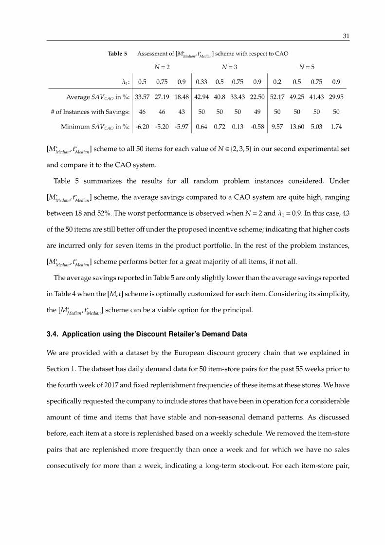
31

Table 5 Assessment of [M∗

Median, t∗

Median] scheme with respect to CAO

N = 2 N = 3 N = 5

λ1: 0.5 0.75 0.9 0.33 0.5 0.75 0.9 0.2 0.5 0.75 0.9

Average SAVCAO in %: 33.57 27.19 18.48 42.94 40.8 33.43 22.50 52.17 49.25 41.43 29.95

# of Instances with Savings: 46 46 43 50 50 50 49 50 50 50 50

Minimum SAVCAO in %: -6.20 -5.20 -5.97 0.64 0.72 0.13 -0.58 9.57 13.60 5.03 1.74

[M∗

Median, t∗

Median] scheme to all 50 items for each value of N ∈ {2,3,5} in our second experimental set

and compare it to the CAO system.

Table 5 summarizes the results for all random problem instances considered. Under

[M∗

Median, t∗

Median] scheme, the average savings compared to a CAO system are quite high, ranging

between 18 and 52%. The worst performance is observed when N = 2 and λ1 = 0.9. In this case, 43

of the 50 items are still better off under the proposed incentive scheme; indicating that higher costs

are incurred only for seven items in the product portfolio. In the rest of the problem instances,

[M∗

Median, t∗

Median] scheme performs better for a great majority of all items, if not all.

The average savings reported in Table 5 are only slightly lower than the average savings reported

in Table 4 when the [M, t] scheme is optimally customized for each item. Considering its simplicity,

the [M∗

Median, t∗

Median] scheme can be a viable option for the principal.

3.4. Application using the Discount Retailer’s Demand Data

We are provided with a dataset by the European discount grocery chain that we explained in

Section 1. The dataset has daily demand data for 50 item-store pairs for the past 55 weeks prior to

the fourth week of 2017 and fixed replenishment frequencies of these items at these stores. We have

specifically requested the company to include stores that have been in operation for a considerable

amount of time and items that have stable and non-seasonal demand patterns. As discussed

before, each item at a store is replenished based on a weekly schedule. We removed the item-store

pairs that are replenished more frequently than once a week and for which we have no sales

consecutively for more than a week, indicating a long-term stock-out. For each item-store pair,

32

Table 6 Parameters of the Four Items Selected from Retailer’s Data Set

Item λ1 µ1 σ1 k1 λ2 µ2 σ2 k2 λ3 µ3 σ3 k3

1 0.89 92.9 19.8 4.69 0.11 161.3 19.8 8.15 - - - -

2 0.78 81.6 16.4 4.98 0.22 187.5 129.1 1.45 - - - -

3 0.9 33.9 9.7 3.49 0.1 71.0 32.9 2.16 - - - -

4 0.56 16.7 4.3 3.88 0.44 29.4 10.6 2.77 - - - -

5 0.78 130.4 23.0 5.67 0.12 41.1 15.2 2.70 0.1 305.3 148.2 2.10

we also removed weeks for which there were no sales for more than one day to avoid censoring

due to short-term stock-outs. For each of the remaining item-store pairs, using the total weekly

demand, we seek to group weeks into different clusters, each cluster corresponding to a different

Normal variate. For this purpose, we used model-based clustering which clusters data based on

Normal mixture modeling (Fraley and Raftery, 2002). The clustering algorithm developed in R for

this purpose (Fraley et. al, 2012) left us with eleven item-store pairs with more than one cluster: ten

with two clusters and one with three clusters. We then carried out routine tests for the fitness of

Wiener Process using the daily demand data. These tests are used to verify that daily demand fits

the Normal distribution, is stationary (using augmented Dickey-Fuller test), and does not exhibit

auto-regression. In the end, we are left with five item-store pairs. Four of these item-store pairs

had two Gaussian density clusters and one had three clusters. There were four distinct items in

three stores. These items were bottled water, UHT processed milk, pasta and margarine. Table 6

lists the mixture probabilities as well as the mean and standard deviation of the best fit clusters

provided by the algorithm.

Figure 2 shows the daily and weekly sales of the first item-store pair in Table 6. The item is a 1/2

liter UHT processed milk. There was no significant seasonality or trend pattern (within week or

within year) in the daily sales. The model based clustering algorithm identified two clusters for the

weekly sales. Six of the weeks belonged to the second cluster (higher sales), while the remaining

weeks belonged to the first cluster. There was no clear indication (such as national holidays or

other calendar effects) that can be used by the retail chain headquarters to explain why there was

33

a higher demand in these six weeks. Our communication with the retail chain, however, suggests

that the store representatives may possess some information to identify the weeks in which their

stores will face higher than usual demand.

0

20

40

60

80

100

120

140

160

180

200

1 8

15

22

29

36

43

50

57

64

71

78

85

92

99

10

6

11

3

12

0

12

7

13

4

14

1

14

8

15

5

16

2

16

9

17

6

18

3

19

0

19

7

20

4

21

1

21

8

22

5

23

2

23

9

24

6

25

3

26

0

26

7

27

4

28

1

28

8

29

5

30

2

30

9

31

6

32

3

33

0

33

7

34

4

35

1

35

8

36

5

37

2

37

9

38

6

Daily Sales Weekly Sales Cluster 1 Cluster 2

Figure 2 Daily and Weekly Sales for Item-Store 1 with Two Demand Clusters

The results of our analysis with these five item-store pairs are presented in Table 7. We use a

cu value of 50 and 100. The latter value is a more realistic scenario for the chain, corresponding

to roughly 20% annual inventory carrying cost per unit and 35% shortage cost per unit. Perfect

alignment is achieved for the first four selected item-store pairs; their demand parameters listed

in Table 6 satisfy the conditions of Theorem 5. In particular, for each of these item-store pairs,

if k1 > k2 (k1 < k2) then σ1 ≤ σ2 (σ2 ≤ σ1). The fifth selected item has three demand clusters and

perfect alignment is not possible. Despite this and even though the parameters of this item-store

pair does not satisfy the conditions of Theorem 6, we observe that [M, t] scheme is preferred over

34

Table 7 Results of the [M, t] Scheme

cu Item IncMt t∗ M∗ SAVCAO t∗Median M∗

Median SAVCAO

50 1 0 1 408 46.49% 0.82 6,249 44.39%

2 0 0.82 7,798 68.36% 68.28%

3 0 0.75 6,249 63.43% 61.85%

4 0 0.78 2,388 41.75% 37.01%

5 0.61% 0.84 9,612 73.45% 72.58%

100 1 0 1 742 45.30% 0.83 13,564 43.30%

2 0 0.83 15,844 68.99% 68.95%

3 0 0.77 13,564 64.86% 63.48%

4 0 0.79 5,127 41.59% 37.32%

5 0.53% 0.85 19,291 68.63% 67.78%

[M]. For this last item-store pair, the retailer can obtain near-perfect alignment; complete demand

information will further reduce the costs only slightly for the retailer, for about 0.5%.

As mentioned in Section 1, this retailer utilizes a CAO system to generate replenishment orders

for each item in each store with some limited override privileges given to store representatives. We

compare the optimal proposed incentive schemes to the CAO system recommendations in Table

7. The first SAVCAO column reports these savings. We observe that such savings can be substantial

(up to 73%) when cu is set to 50 or 100. The median of the t∗ and M∗ values when cu = 50 are

0.82 and 6249, respectively. The same values for cu = 100 are 0.83 and 13564, respectively. The last

column of Table 7 reports SAVCAO values when these median values are used for all five items for

ease of implementation. Even under this case, substantial savings can still be achieved. The results

show that this chain can have significant savings if the headquarters can use a proper scheme for

incentive alignment and delegate replenishment decisions to more informed store representatives.

4. Conclusion

We consider a problem faced by a principal who delegates the replenishment decisions of a

periodically ordered item to an agent. The principal has incomplete demand information and

35

cannot observe lost sales and needs an incentive scheme so that the agent orders a quantity that

minimizes the principal’s overage and underage costs. The demand process is assumed to be a

Wiener Process; the agent knows which particular Wiener Process will take place prior to ordering

whereas the principal only knows the set of possible Wiener Processes and their probabilities. We

propose a scheme where the performance score of the agent depends on how much inventory

remains at the end of period and whether there is any stock-out at a pre-specified instant prior

to or at the end of the period. We show that when the Wiener Processes share the same variance,

the principal can perfectly align the agent’s incentives by inspecting the stock-out at the end of

the period and setting a proper penalty for a potential stock-out to be deducted from the agent’s

performance score. Under some mild conditions and when there are only two possible processes,

perfect alignment is still possible, but interestingly requires the inspection of stock-out before the

period ends. In general, such early inspection schemes may lead to strictly better results than only

relying on stock-out information at the end of the period. Our numerical results on synthetic and

real data show that the scheme we suggest leads to near-perfect alignment and significant savings

over centralized ordering based on incomplete demand information.

There may be many avenues for further research in this area. First, it may be interesting to study

more general demand processes and investigate settings where the incentive schemes proposed

here still lead to perfect or near-perfect alignment. Second, new schemes may be developed under

the assumptions of this paper. For example, in some settings it may be possible to detect the

exact time the store runs out of stock and design an incentive scheme based on the stock-out

time. However, one may argue that these schemes may be complex and hard to implement in

practice. Finally, this paper handles the multiple items case in a heuristic manner by solving the

problem separately for each item and using the median values of the incentive parameters for all

items. While the results for this heuristic are impressive, determining the common [t,M] pair that

minimizes the principal’s underage and overage costs over all items can be posed as an interesting

and challenging optimization problem.

36

References

Agrawal, N., Smith, S. A. 1996. Estimating negative binomial demand for retail inventory man-

agement with unobservable lost sales. Naval Research Logistics. 43, 839–861.

Akan, M., Ata, B. and Lariviere, M.A., 2011. Asymmetric information and economies of scale in

service contracting. Manufacturing & Service Operations Management. 13, 58–72.

Anderson, E. T., Fitzsimons, G. J., Simester, D. Measuring and mitigating the costs of stockouts.

Management Science. 52, 1751–1763.

Aneja, Y., Noori, A. H. 1987. The optimality of (s, S) policies for a stochastic inventory problem

with proportional and lump-sum penalty cost. Management Science. 33, 750–755.

Anupindi, R., Dada, M. Gupta, S. 1998 Estimation of consumer demand with stock-out based

substitution: An application to vending machine products. Marketing Science. 17, 406–423.

Babich, V., Li, H., Ritchken, P. and Wang, Y., 2012. Contracting with asymmetric demand informa-

tion in supply chains. European Journal of Operational Research. 217, 333–341.

Bagnoli, M., Bergstrom, T. 2005. Log-concave probability and its applications. Economic Theory. 26,

445–469.

Baldenius, T., Reichelstein, S. 2005. Incentives for efficient inventory management: The role of

historical cost. Management Science. 51 1032–1045.

Bell, P. C., Noori, A. 1984. Foreign currency inventory management in a branch bank. Journal of

Operational Research Society. 35, 513–525.

Benkherouf, L., Sethi, S. P. 2010. Optimality of (s,S) policies for a stochastic inventory model with

proportional and lump-sum shortage costs. Operations Research Letters. 38, 252–255

Cetinkaya, S., Parlar, M. 1989. Optimal myopic policy for a stochastic inventory problem with

fixed and proportional backorder costs. European Journal of Operational Research. 110, 20–41.

Chen, F., 2000. Sales-force incentives and inventory management. Manufacturing & Service Opera-

tions Management. 2, 186–202.

37

Chen, F., 2001. Information sharing and supply chain coordination. In: de Kok, A.G., Graves,

S.C.(Eds.), Handbooks in Operations Research and Management Science: Supply Chain Management.

Chapter 7. 341-413.

Chu, L.Y. and Lai, G., 2013. Salesforce contracting under demand censorship. Manufacturing &

Service Operations Management. 15, 320–334.

Coca-Cola Research Council. 1996. Where to look for incremental gains: The retail prob-

lem of out-of-stock merchandise, The Coca-Cola Research Council, Atlanta, GA, accessed

at http://www.ccrrc.org/1996/02/24/where-to-look-for-incremental-sales-gains/ as of January 30,

2017.

Corsten, D., Gruen, T. 2004. Stock-outs cause walkouts. Harvard Business Review. 82, 26–28.

Dai, T., Jerath, K. 2013. Salesforce compensation with inventory considerations. Management Sci-

ence. 59, 2490–2501.

DeHoratius, N., Raman, A. 2007. Store manager incentive design and retail performance: An

exploratory investigation. Manufacturing & Service Operations Management. 9, 518–534.

ECR Europe. 2003. ECR Optimal shelf availability, increasing shopper satisfaction at the moment

of truth, ECR Europe, Brussels, accessed at http://ecr-all.org/files/pub 2003 osa blue book.pdf

as of January 30, 2017.

FMI/GMA Trading Partner Alliance. 2015. Solving the out-of-stock problem, accessed at

http://www.gmaonline.org/file-manager/15032FMIN TPA OutofStock v41.pdf as of January 30,

2017.

Fraley, C., Raftery, A. E. 2002. Model-based clustering, discriminant analysis, and density estima-

tion. Journal of the American Statistical Association. 97, 611–631.

C. Fraley, C., Raftery, A. E., Murphy, T. B., Scrucca, L. 2012. mclust Version 4 for R: Normal mixture

modeling for model-based clustering, classification, and density estimation. Technical Report

No. 597, Department of Statistics, University of Washington.

38

Geng, Q. and Minutolo, M.C., 2010. Failure fee under stochastic demand and information asym-

metry. International Journal of Production Economics. 128, 269–279.

Gruen, T. W., Corsten, D. 2008. A comprehensive guide to retail out-of-stock reduction in

the fast-moving consumer goods industry, available at http://itsoutofstock.com/wpcontent/

uploads/2013/04/OOS-Guide-2008-Revision.pdf.

Gruen, T. W., Corsten, D., Bharadwaj, S. 2002. Retail out of stocks: A world-

wide examination of extent, causes and consumer responses, Grocery Manu-

facturers of America, Washington, DC, available at: http://itsoutofstock.com/wp-

content/uploads/2013/04/GMA 2002 Worldwide OOS Study.pdf

Kaplan, R. S., Norton, D. P. 1992. The balanced scorecard measures that drive performance.

Harvard Business Review, Jan/Feb, 71-79.

Khanjari, N. E., Iravani, S. and Shin, H., 2013. The impact of the manufacturer-hired sales agent on

a supply chain with information asymmetry. Manufacturing & Service Operations Management.

16, 76–88.

Laffont, J-J., Martimort, D. 2009. The theory of incentives: the principal-agent model. Princeton

University Press.

Lee, H., Whang, S. 1999. Decentralized multi-echelon supply chains: incentives and information.

Management Science. 45, 633–640.

Marshall, A. W., Olkin, I. 2007. Life distributions: structure of nonparametric, semiparametric, and

parametric families. Springer.

Narayanan, V. G., Raman, A. 2004. Aligning incentives in supply chains. Harvard Business Review.

82, 94–102.

Parzen E. 1979. Nonparametric statistical data modeling. Journal of the American Statistical Associa-

tion. 74, 105–121.

Patel, J. K., Read, B. C. B. 1982. Handbook of the normal distribution. Statistics: textbooks and

monographs. 40. New York and Basel.

39

Peckham, J. O. 1963. The consumer speaks. Journal of Marketing. 27, 21–26.

Porteus, E.L. 2002. Foundations of stochastic inventory theory. Stanford University Press.

Rao, U.S. 2003. Properties of the periodic review (R, T) inventory control policy for stationary,

stochastic demand. Manufacturing & Service Operations Management. 5, 37–53.

Rudi, N., Groenevelt, H., Randall, T.R. 2009. End-of-period vs. continuous accounting of inventory-

related costs. Operations Research. 57, 1360–1366.

Schenk-Mathes, H.Y., 1995. The design of supply contracts as a problem of delegation. European

Journal of Operational Research. 86, 176–187.

Sieke, M.A., Seifert, R.W., Thonemann, U.W., 2012. Designing service level contracts for supply

chain coordination. Production and Operations Management. 21, 698–714.

Tukey, J. W. 1965. Which part of the sample contains the information? Proceedings of the National

Academy of Sciences of the United States of America. 53, 127–134.

van Ackere, A., 1993. The principal/agent paradigm: Its relevance to various functional fields.

European Journal of Operational Research. 70, 83–103.

van Donselaar, K. H., Gaur, V., van Woensel, T., Broekmeulen, R. A. C. M., Fransoo, J. C. 2010.

Ordering behavior in retail stores and implications for automated replenishment. Management

Science, 56, 5, 766–784.

Witcher, B. J., Chau, V. S. 2008. Contrasting uses of balanced scorecards: case studies at two UK

companies. Strategic Change, 17 101-114.

Xu, K., Yin, R., Dong, Y., 2016. Stockout recovery under consignment: The role of inventory

ownership in supply chains. Decision Sciences. 47, 94–124

Zhang, H., Zenios, S., 2008. A dynamic principal-agent model with hidden information: Sequential

optimality through truthful state revelation. Operations Research. 56, 681–696.