stock prices, news, and economic fluctuations - (macro)economics

Stock Prices, News, and Economic Fluctuations

By PAUL BEAUDRY AND FRANCK PORTIER*

There is a huge literature suggesting that stock price movements reflect the market's expectation of future developments in the economy. As a test of standard valuation models, Eugene F. Fama (1990) shows that monthly, quarterly, and annual stock returns are highly correlated with future production growth rates for the 1953-1987 period. This result is confirmed on a extended sample (1889-1988) by G. William Schwert (1990). Both authors argue that the relationship between current stock returns and future production growth reflects expectations about future cash flow that is impounded in stock prices. There is also a huge literature, and a long tradition in macroeconomics (from Arthur C. Pigou, 1927, and John Maynard Keynes, 1936, to the survey of Jess Benhabib and Roger E. A. Farmer, 1999) suggesting that changes in expectation may be an important element driving economic fluctuations.

Given this, it is surprising that the empirical macro literature-especially the VAR-based literature-rarely exploits stock price movements to expand our understanding of the role of expectations in business cycle fluctuations. In this paper, we take a step in this direction by showing how stock price movements, in conjunction with movements in total factor productivity (TFP), can be fruitfully used to help shed new light on the forces driving business cycle fluctuation.

The empirical strategy we adopt in this paper is to perform two different orthogonalization schemes as a means of identifying properties of

the data that can then be used to evaluate theo- ries of business cycles. Let us be clear that our empirical strategy is a purely descriptive device which becomes of interest only when its implications are compared with those of structural models. The two orthogonalization schemes we use are based on imposing sequentially, not simultaneously, either impact or long-run restrictions on the orthogonalized moving average representation of the data. The primary system of variables that interests us is one composed of an index of stock market value and measured TFP. Our interest in focusing on stock market information is motivated by the view that stock prices are likely a good variable for capturing any changes in agents' expectations about future economic conditions.

The two disturbances we isolate with our procedure are: a disturbance that represents innovations in stock prices, which are orthogonal to innovations in TFP; and a disturbance that drives long-run movements in TFP. The main intriguing observation we uncover is that these two disturbances-when isolated separately without imposing orthogonality-are found to be almost perfectly colinear and to induce the same dynamics. We also show that these colinear shock series cause standard business cycle comovements and explain a large fraction of business cycle fluctuations. Moreover, when we use measures of TFP which control for variable rates of factor utilization, as, for example, when we use the series constructed by Basu et al. (2002), we find that our shock series anticipates TFP growth by several years.

In order to interpret the result from our empirical exercise, we present a model where technological innovations affect productive capacity with delay, and show how such a model can explain quite easily the patterns observed in the data. In particular, our evidence suggests that business cycles may be driven to a large extent by TFP growth that is heavily anticipated by economic agents, thereby leading to what might be called expectation-driven booms. Hence, our empirical results suggest that an important faction of business cycle fluctuations may be driven by

* Beaudry: CRC University of British Columbia, 997- 1873 East Mall, Vancouver, BC, Canada V6T 121, and National Bureau of Economic Research (e-mail: [email protected]); Portier: Universitd de Tou- louse, 21 Allde de Brienne, F-31042 Toulouse, France

(GREMAQ, IDEI, LEERNA, Institute Universitaire de France and CEPR) (e-mail: [email protected]). The authors thank Susanto Basu, Larry Christiano, Roger Farmer, Robert Hall, Richard Rogerson, Julio Rotemberg, and participants at seminars at CEPR ESSIM 2002, SED Paris 2003, Bank of Canada, Bank of England, the Fed- eral Reserve of Philadelphia, the National Bureau of Economic Research, University of Berlin, Universit6 du Qudbec g Montrdal, Universit6 de Toulouse, and CREST for helpful comments.

1293

1294 THE AMERICAN ECONOMIC REVIEW SEPTEMBER 2006

changes in expectations-as is often suggested in the macro literature-but these changes in expectations may well be based on fundamentals since they anticipate future changes in productivity.

The remaining sections of the paper are struc- tured as follows. In Section I, we present our empirical strategy and show how it can be used to shed light on the sources of economic fluctuation. In Section II, we present the data and in Section III, we implement our strategy using postwar U.S. data. Finally, Section IV offers some concluding comments.

I. Using Impact and Long-run Restrictions Sequentially to Learn About Macroeconomic

Fluctuations

The object of this section is to present a new means of using orthogonalization techniques- i.e., impact and long-run restrictions-to learn about the nature of business cycle fluctuations. Our idea is not to use these techniques simultaneously, but instead to use them sequentially. In particular, we will want to apply this sequenc- ing to describe the joint behavior of stock prices (SP) and measured TFP, in a manner that can be easily interpretable. The main characteristic of stock prices we want to exploit is that it is an unhindered jump variable.

A. Two Orthogonalization Schemes

Let us begin our discussion from a situation where we already have an estimate of the reduced form moving average (Wold) representation for the bivariate system (TFP,, SP,) (for ease of presentation we neglect any drift terms):

/ TFP,\t -(L ,t ASP, J =

C(L)y2,t]'} where L is the lag operator, C(L) = I + I CiL', and fn is the variance covariance matrix of 4. Furthermore, we assume that the system has at least one stochastic trend and therefore C(1) is not equal to zero. In effect, most of our analysis will be based on a moving average representation derived from the estimation of a vector error correction model (VECM) for TFP and stock prices.

Now consider deriving from this Wold representation alternative representations with orthogonalized errors. As is well known, there are

many ways of deriving such representations. We want to consider two of these possibilities, one that imposes an impact restriction on the representation and one that imposes a long-run restriction. In order to see this clearly, let us denote these two alternative representations by

(1) A TFP, = F(L) Ie,

ASP e2,t

ASTFP, /E (2) ASP,

= f(L) E2,t

where F(L) and the variance covariance matrices of e and E are identity matrices. In order to get such a representation, say in the case of (1), we need to find the F matrices that solve the following system of equations:

r Fo0O =

fi Fi C,,Fo for i > 0.

Since this system has one more variable than equations, however, it is necessary to add a restriction to pin down a particular solution. In case (1), we do this by imposing that the 1, 2 element of Fo is equal to zero; that is, we choose an orthogonalization where the second disturbance e2 has no contemporaneous impact on TFPt. In case (2), we impose that the 1, 2 element of the long-run matrix Fi equals zero; that is, we choose an orthogonalization where the disturbance Z2 has no long-run impact on TFP, (the use of this type of orthogonalization was first proposed by Olivier Jean Blanchard and Danny Quah, 1989). We use these two different ways of organizing the data to help evaluate different classes of economic models and indicate directions for model refor- mulation. For example, a particular theory may imply that the correlation between the shocks e2 and

El is close to zero and that their associated

impulse responses are different. Therefore, we can evaluate the relevance of such a theory by examining the validity of its implications along such a dimension.

In order to clarify the potential usefulness of such a procedure, consider a simple canonical model of fluctuations driven by random walk technology shocks and random walk monetary shocks with orthogonal innovations 7 1,t and

7l2,t. The environment envisaged is a standard

VOL 96 NO. 4 BEAUDRY AND PORTIER: STOCK PRICES, NEWS, AND ECONOMIC FLUCTUATIONS 1295

New Keynesien model with monopolistic com- petition in the intermediate good sector and preset prices. The value of firms (the stock market value) in this economy is the discounted sum of profits of intermediate good producers. In such an economy, output and firm profits will be affected by unexpected money and the level of technology. Hence, as is easy to verify,' such a model delivers a structural moving average representation for TFP, and stock market value (SP,) where the mapping between the structural shocks (r7) and the associated shocks (e and E) is:

(3) e, = ' 2, e2 =2rh1, l =r72.

The important aspect of this model is that the derived e2 shock, which under this theory should correspond to the money shock, is predicted to be orthogonal to E1, which should be the surprise increase in productivity. Therefore, looking at whether this type of pattern is found in the data provides a means of evaluating the relevance of such a class of models, that is, models where surprise technological disturbances are a potentially important source of fluctuations.

A Model with Delayed Response of Innova- tion on Productivity.-Let us now consider an alternative setting where stock prices continue to be a discounted sum of future profits, but where technological innovations no longer im- mediately increase productivity. Instead they only increase productive capacity over time. The objective of this example is to emphasize what such an environment predicts regarding the correlation between 82 and

E1, derived using

sequential impact and long-run restrictions. To this end, let us assume that log TFP, denoted 0, is composed of two components: a nonstationary component Dt and a stationary component vt. The component v, can be thought of either as a measurement error or as a temporary technology shock. For the discussion, we will treat

vt as

a temporary shock to 0, although the measurement error interpretation has the same implications. In contrast, the component Dr is the

1 See Beaudry and Portier (2004).

permanent component of technology and is assumed to follow the process given below:

6, = D, + v,

D, = diti

(4) i=O

d= 1- 8, 0 86 < 1 vt = pvt-1 + "l2,t, O <-p < 1.

We will call the process for D, a diffusion process, since an innovation ml is restricted to have no immediate impact on productive capacity (do = 0), the effect of the technological innovation on productivity is assumed to grow over time di+,), and the long-run effect is normalized to one. In contrast to the common random walk assumption for the permanent component of TFP, such a process allows for an S-shaped response of TFP to a technological innovation. Now consider the implied structural moving average for ATFP and ASP, assuming that prices and wages are flexible, so that the only two innovations affecting real variables are the innovations to Dr and vt,. In this case, per- forming our short-run and long-run identification on this system, the relationship between the identified errors e,, and the structural errors m, are:

(5) E1 = rl~, ~2 = r/2.

In particular, such a model predicts 82 to be colinear to Z1.

This diffusion model is different from a baseline New Keynesien model in that, even before technological opportunities have actually expanded an economy's production possibility set, forward-looking variables-such as stock prices-are incorporating this possibility. If this class of models is relevant, the long-run restriction used to derive the orthogonal moving average representation given by fi and 8 still implies that E1 can be interpreted as a technological shock, but now it implies that this shock has zero effect on productivity on impact; that is, if productivity changes are anticipated, then by definition of an anticipated shock, the actual shock has zero effect on impact on TFPt. Hence, under this type of model, e2 and El are predicted to be colinear as they both should capture the effect of anticipated changes in technological opportunities.


Moreover, the impulse responses associated with 82 and l should be identical.

II. Data and Specification Issues

Our empirical investigation will use U.S. data over the period 1948-Q1 to 2000-Q4 (the data were collected in August 2002). The two series that interest us for our bivariate analysis are an index of stock market value (SP) and a measure of total factor productivity (TFP). Later, we will consider larger systems that also include consumption, investment, and hours worked, and therefore we also present the source of these data.

The stock market index we use is the quarterly Standards & Poors 500 Composite Stock Prices Index, deflated by the seasonally adjusted implicit price deflator of GDP in the nonfarm private business sector and transformed in per capita terms by dividing it by the population age 15 to 64. As the population series is annual, it has been interpolated assuming constant growth within the quarters of the same year. We denote the log of this index by SP.

The construction of our baseline TFP series is relatively standard. We restrict our atten- tion to the nonfarm private business sector. From the U.S. Bureau of Labor Statistics (BLS), we retrieved two annual series: labor share (sh) and capital services (KS), which measure the services derived from the stock of physical assets and software. The capital services series has been interpolated to obtain a quarterly series, assuming constant growth within the quarters of the same year. Output (Y) and hours (H) are quarterly and seasonally adjusted nonfarm business measures, from 1947-Q1 to 2000-Q4 (also from the BLS). We then con- struct a measure of (log) TFP as TFP, = log(Y/ I-JhKS: where sh is the average level of the labor share over the period.

The consumption measure (C) we use is the per capita value of real personal consumption of nondurable goods and services, while investment (1) is the per capita value of the sum of real personal consumption of durable goods and real fixed private domestic investment.

Specification.-From our data on TFP and SP, we first want to recover the Wold moving average representation for ATFP and ASP. Since from unit root tests (not reported here)

and cointegration tests, we found that SP and TFP are likely cointegrated I(1) processes, a natural means of recovering the Wold representation is by inverting a VECM. In a VECM framework, however, one must be careful to properly identify the matrix of cointegration relationships in order to avoid mispecification. In effect, as emphasized in James D. Hamilton (1994), if one is worried about potential mispecification, it may be best to estimate the VECM allowing for the matrix of cointegrating relationships to be of full rank-which corre- sponds to estimating the system in level. Then one can estimate the VECM with a matrix of cointegration relationships, which is of reduced rank, and examine whether the resulting Wold representation is similar to that found by estimating the system in levels. In the following, we adhere to this principal by reporting results based on a Wold representation achieved by inverting a VECM, having verified that the results are robust to estimating the system in levels. Since we want to avoid mispecification bias due to an omitted cointegration relationship, our approach to testing for a cointegrating relationship is conservative, in the sense of testing from a more (HO) cointegrating relationship to less (H1). To this end, we used the test proposed by Jukka Nyblom and Andrew Har- vey (2000) to test for cointegration. This procedure indicates that cointegration between SP and TFP could not be rejected at the 5-percent level and therefore we adopted the VECM specification as our benchmark specification.

The second specification choice is related to the number of lags to include in the VECM. Again, our strategy is not to impose much on the data. According to the likelihood ratio test, two or five lags appear preferable-when testing in a descendant way for the optimal number of lags from two years up to one quarter. When testing one against the other, five is preferred to two. We therefore choose to work with five lags since this seemed to us large enough not to place too many restrictions on the data. It is, nevertheless, worth noting that all our results are robust to adopting a two-lag specification. One of the drawbacks of the way we have proceeded to choose this baseline specification is that we have examined the issues of cointegration rank and lag length sequentially. As has been shown by Seren Johansen (1992), such a procedure can have undesirable properties. As a

VOL. 96 NO. 4 BEAUDRY AND PORTIER: STOCK PRICES, NEWS, AND ECONOMIC FLUCTUATIONS 1297

means of getting around this problem, John C. Chao and Peter C. B. Phillips (1999) propose a Posterior Information Criterion (PIC) that allows us to jointly select the lag length and cointegration rank of a VECM. The use of the PIC in the case at hand suggests a very parsimonious model with no cointegration and only one lag. The difference with the previous find- ing is not too surprising, since the PIC imposes a strong penalty for extra parameters. In order to select between the extremely parsimonious specification suggested using the PIC and the less restrictive specification discussed above, we performed a likelihood ratio test. Our find- ing was that specification selected by the PIC was rejected in favor of specifications with cointegration and more lags. Therefore, given our economic prior suggesting that TFP and stock prices are likely cointegrated, and given our desire not to impose unnecessary restrictions, we choose to proceed with the cointegration specification with five lags of data.2

III. Results in a Bivariate System

A. Preliminary Results

We began by estimating a VECM for (TFP, SP) with one cointegrating relationship and recover two orthogonalized shock series cor- responding to the e and E discussed in Section I, that is, e was recovered by imposing an impact restriction (a restriction on Fo) and was recovered by imposing a long-run restriction. The level impulse responses on (TFP, SP) associated with the E2 shock and the shock are displayed in Figure 1. The striking observation is that these responses appear very similar when comparing one orthogonalization to another. More specifically, the dynamics associated with the e] shock-which by construction is an innovation in stock prices which are contemporaneously orthogonal to TFP-seem to permanently affect TFP, while the dynamics associated with the

O shock-which by construction has a permanent effect on TFP-have essentially no impact effect on TFP (the point estimate indicates a slight negative effect) but have a

substantial effect on SP. On the one hand, these results suggest that 82 contains information about future TFP growth, which is instan- taneously and positively reflected in stock prices.3 On the other hand, they suggest that permanent changes in TFP are reflected in stock prices before they actually increase productive capacity.

The similarity between the effects of these two shocks derives from the quasi-identity of the 82 shock and the

E1 shock, as shown in Figure 2, which simply plots 82,t against

El,,. In effect, the correlation coefficient between these two series is 0.97 (with a standard deviation of 0.006), that is, these two orthogonalization techniques recover essentially the same shock series.4 The interesting question then becomes, what kind of structural macroeconomic model is consistent with these two orthogonalization techniques generating the same shock series? As we have discussed, this observation runs counter to simple models where technological improvements are modelled as sur- prises, since these models generally imply that e2 and

E1 should be orthogonal. In contrast, this pat-

tern appears consistent with the view-which we call the news view-that improvements in productivity are generally anticipated by market participants due to a lag between the recognition of a technological innovation and its eventual impact on productivity.5

Let us emphasize that, if we interpret the current results as reflecting a diffusion process from innovation to productivity, it suggest that diffusion is rather fast. In effect, in Figure I we observed that measured TFP starts growing quickly after the initial increase in stock prices, with the peak obtained after approximately four

2 Note that the type of models discussed in Section I generally implies that SP, and TFP, are cointegrated.

3The observation in Figure 1, whereby TFP increases following an innovation in SP, indicates that stock prices Granger cause TFP. In effect, we also directly performed the test of whether SP Granger causes TFP in this system and we found that such causality could not be rejected at the 1-percent level.

4 The observation that e2 and fi are highly correlated suggests testing the overidentification restriction obtained by combining the short-run and long-run restrictions. When we perform this test within a minimum distance framework, we find that the overidentifying restriction is not rejected at conventional values (p-value = 0.90).

5In Beaudry and Portier (2004), we document the robustness of these observations to a different choice of lag length and to estimating the system in levels rather than in VECM form.


Percent

deviation

0.8

0.7

0.6

0.5

0.4

0.3

0.2

0.1

0

-0.1 0 5 10 15 20

Quarters

TFP

Percent

deviation

11

10

9

8

7

6

50 5 10 15 20 Quarters

Stock prices

FIGURE 1. IMPULSE RESPONSES TO SHOCKS 82 AND Eg IN THE (TFP, SP) VECM

Notes: In both panels of this figure, the bold line represents the point estimate of the responses to a unit e2 shock (the shock that does not have instantaneous impact of TFP in the short-run identification). The line with circles represents the point estimate of the responses to a unit , shock (the shock that has a permanent impact on TFP in the long-run identification). Both identifications are done in the baseline bivariate specification (five lags and one cointegrating relation). The unit of the vertical axis is percentage deviation from the situation without shock. Dotted lines represent the 10-percent and 90-percent quantiles of the distribution of the impulse response functions (IRFs) in the case of the short-run identification, this distribution being the Bayesian simulated distribution obtained by Monte-Carlo integration with 2,500 replications, using the approach for just-identified systems discussed in Thomas J. Doan (1992).

quarters. One potential problem with this observation, however, is that our measure of TFP may be an improper measure of technological opportunities since it does not account for potential changes in rates of factor utilization. Therefore, it may be the case that in response to a technological innovation, properly measured TFP does not increase for a substantial period of time, but that mismeasured TFP responds rap- idly due to changes in factor utilization. Hence, in the next subsection, we explore the robustness of our observations with respect to alternative measures of TFP.

B. Controlling for Variable Rates of Factor Utilization

There is a vast literature regarding how best to calculate TFP in order to obtain a good reflection of changes in production opportunities. In particular, the literature on this issue emphasizes several potential problems with the type of measure of TFP we used in the previous section. For example, our previous measure may be inappropriate due to our lack of correction for variable rates of capital utilization, labor hoarding, or composition bias. One attempt to control for most of these biases can

be found in the TFP series produced by Susanto Basu et al. (2002) (hereafter BFK). This series has the advantage of being constructed from disaggregated data which control for variable rates of factor utilization. For this reason it appears as a good

I

4

3

2

1

0

-1

-2

-3

-4 -4 -3 -2 -1 0 1 2 3 4

E2

FIGURE 2. PLOT OF 82 AGAINST 1 IN THE

(TFP, SP) VECM

Notes: This figure plots 82 against 81. Both shocks are obtained from the baseline bivariate specification (five lags and one cointegrating relation). The straight line is the 45-degree line.


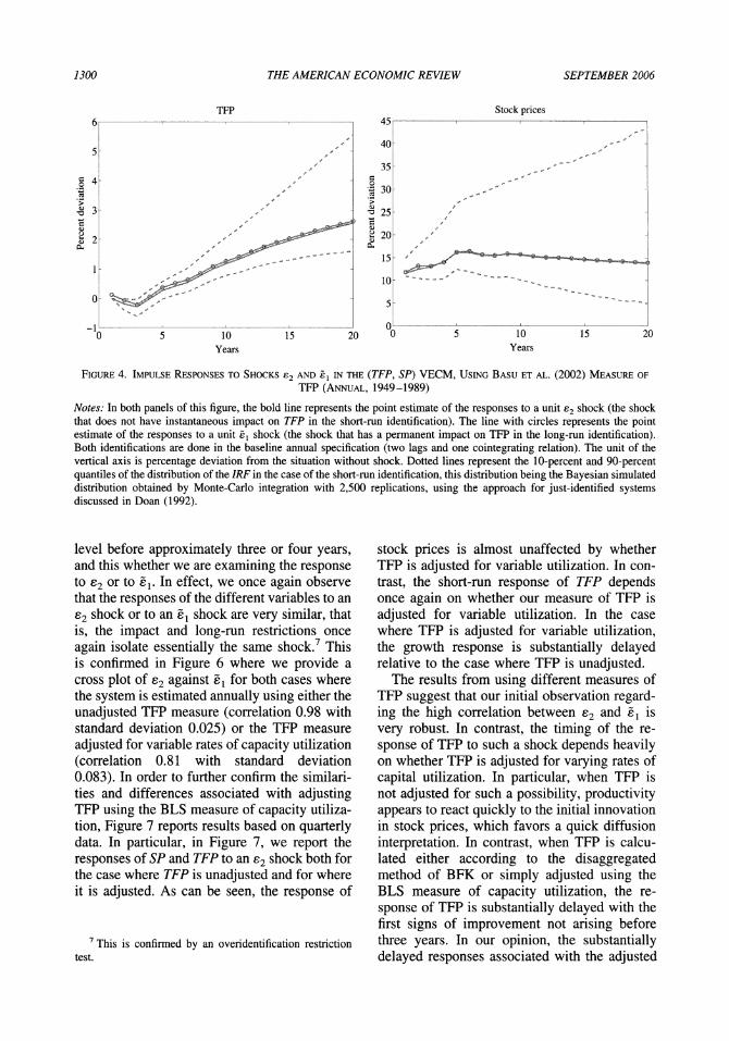
alternative series to examine the robustness of our previous results. It also has some drawbacks, however. First, it is an annual rather than quarterly series. Second, it covers only the period 1948 to 1989. Notwithstanding these drawbacks, we will begin this section by exploiting this series to see whether it changes any of our previous results. To this end, we estimated an annual bivariate VECM representation for stock prices and the BFK measure of TFP using three lags of data. The stock prices used are end-of-period prices. The results from sequentially imposing our impact and long- run restrictions to obtain orthogonal representations are given in Figures 3 and 4.

In Figure 3, we present the cross plot of e2 and Z, recuperated from the livariate representation of TFP and SP using the BFK data. As can be seen, the two innovations are very highly correlated (0.989 with standard deviation 0.025), suggesting that both identification schemes isolate essentially the same shock.6 In Figure 4, we present the impulse responses for TFP and SP associated with the innovations e2 and

E1. Although the responses to both these

shocks are once again very similar, the response of TFP is quite different from our previous observations. In effect, we now see that following an increase in stock prices, TFP does not increase for several years. The point estimates actually suggest that TFP starts growing only four years after the initial rise in the stock market. This long lag between stock price increases and the increase in TFP is potentially consistent with a delayed impact of technological innovation on productivity, where the diffusion now appears quite slow, while it appeared to be rather quick with a less sophis- ticated measure of TFP.

As we indicated previously, there are two potential drawbacks with the BFK measure of TFP: it is annual and covers a limited period. As an alternative to the BFK measure, we constructed an adjusted TFP measure, which we will denote by TFPA, using the BLS measure of capacity utilization (CU,) to adjust our measure of capital services. This adjusted TFP measure is calculated as TFPt =

log(Y/Heh(CUKS)'

Iw

4

3

2

1

0

-1

-2

-3

-4 -4 -3 -2 -1 0 1 2 3 4

E2

FIGURE 3. PLOT OF 82 AGAINST Zl IN THE (TFP, SP) VECM, USING BASU ET AL. (2002) MEASURE OF TFP

(ANNUAL.I 1949-19891

Notes: This figure plots e2 against f1".

Both shocks are obtained from the baseline annual specification (two lags and one cointegrating relation). The straight line is the 45-degree line.

Since the BLS measure of capital utilization is based mainly on manufacturing data, this correction is not above criticism. Nevertheless, it is an alternative worth exploiting to see how results based on this data compare to those based on either the BFK data or on our unadjusted TFP data. In order to make these compar- isons, we first performed our orthogonalizations on annual bivariate VAR over the period 1948 to 2000 using either the pair (TFP,, SP,) or

(TFPt, SP,), where TFP refers to our original

unadjusted TFP series, while TFPA refers to our series adjusted for variable rates of factor utilization. In Figure 5, we superimpose the responses of TFP and stock prices to the orthogonalized shocks e2 and

Z1 estimated for

each system. In the case where we use the annualized unadjusted TFP data, we see that measured TFP increases quickly after the innovation in stock prices, reaching a peak after two years, decreasing slightly afterward, and then resuming growth after about four years. This is quite similar to what was observed when the quarterly version of this data was used. In contrast, the results based on the TFP data adjusted for variations in the rate of capacity utilization (TFPA) are quite different from those based on unadjusted data, while interestingly they resem- ble the results obtained using the BFK data. In effect, we see that following the initial rise in stock prices, TFPA does not overtake its initial

6 The test of the overidentification restriction obtained by combining the long-run and short-run restrictions has a p-value of 0.83.


6

5

4

3

2

1

0

-1 0 5 10 15 20

Years

TFP Stock prices 45

40

35

30

25

20

15

10

5

0 0 5 10 15 20

Years

FIGURE 4. IMPULSE RESPONSES TO SHOCKS 82 AND Tl IN THE (TFP, SP) VECM, USING BASU ET AL. (2002) MEASURE OF

TFP (ANNUAL, 1949-1989)

Notes: In both panels of this figure, the bold line represents the point estimate of the responses to a unit 82 shock (the shock that does not have instantaneous impact on TFP in the short-run identification). The line with circles represents the point estimate of the responses to a unit fi shock (the shock that has a permanent impact on TFP in the long-run identification). Both identifications are done in the baseline annual specification (two lags and one cointegrating relation). The unit of the vertical axis is percentage deviation from the situation without shock. Dotted lines represent the 10-percent and 90-percent quantiles of the distribution of the IRF in the case of the short-run identification, this distribution being the Bayesian simulated distribution obtained by Monte-Carlo integration with 2,500 replications, using the approach for just-identified systems discussed in Doan (1992).

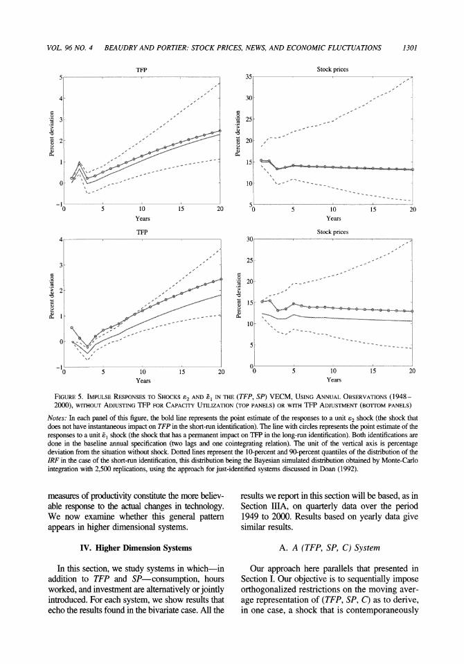
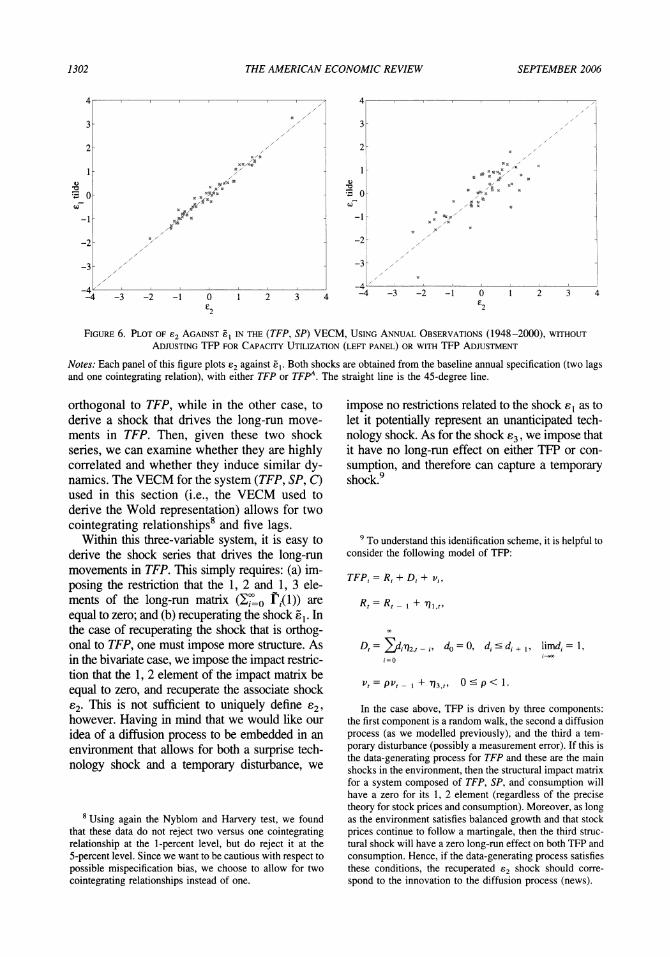
level before approximately three or four years, and this whether we are examining the response to 82 or to EZ. In effect, we once again observe that the responses of the different variables to an 82 shock or to an O shock are very similar, that is, the impact and long-run restrictions once again isolate essentially the same shock.7 This is confirmed in Figure 6 where we provide a cross plot of e2 against El for both cases where the system is estimated annually using either the unadjusted TFP measure (correlation 0.98 with standard deviation 0.025) or the TFP measure adjusted for variable rates of capacity utilization (correlation 0.81 with standard deviation 0.083). In order to further confirm the similari- ties and differences associated with adjusting TFP using the BLS measure of capacity utilization, Figure 7 reports results based on quarterly data. In particular, in Figure 7, we report the responses of SP and TFP to an e2 shock both for the case where TFP is unadjusted and for where it is adjusted. As can be seen, the response of

7 This is confirmed by an overidentification restriction test.

stock prices is almost unaffected by whether TFP is adjusted for variable utilization. In contrast, the short-run response of TFP depends once again on whether our measure of TFP is adjusted for variable utilization. In the case where TFP is adjusted for variable utilization, the growth response is substantially delayed relative to the case where TFP is unadjusted.

The results from using different measures of TFP suggest that our initial observation regarding the high correlation between 82 and ., is very robust. In contrast, the timing of the response of TFP to such a shock depends heavily on whether TFP is adjusted for varying rates of capital utilization. In particular, when TFP is not adjusted for such a possibility, productivity appears to react quickly to the initial innovation in stock prices, which favors a quick diffusion interpretation. In contrast, when TFP is calculated either according to the disaggregated method of BFK or simply adjusted using the BLS measure of capacity utilization, the response of TFP is substantially delayed with the first signs of improvement not arising before three years. In our opinion, the substantially delayed responses associated with the adjusted

Percent

deviation

Percent

deviation


TFP 5

4

3

2

1

0

-I 0 5 10 15 20

Years

35

30

25

20

15

10

5 0 5 10 15 20

Years

Stock prices

Stock prices 30

25

20

15

10

5

0 0 5 10 15 20

Years

TFP 4

3

2

1

0

-1 0 5 10 15 20

Years

FIGURE 5. IMPULSE RESPONSES TO SHOCKS £2 AND 81 IN THE (TFP, SP) VECM, USING ANNUAL OBSERVATIONS (1948- 2000), WITHOUT ADJUSTING TFP FOR CAPACITY UTILIZATION (TOP PANELS) OR WITH TFP ADJUSTMENT (BOTTOM PANELS)

Notes: In each panel of this figure, the bold line represents the point estimate of the responses to a unit E2 shock (the shock that does not have instantaneous impact on TFP in the short-run identification). The line with circles represents the point estimate of the responses to a unit Ez shock (the shock that has a permanent impact on TFP in the long-run identification). Both identifications are done in the baseline annual specification (two lags and one cointegrating relation). The unit of the vertical axis is percentage deviation from the situation without shock. Dotted lines represent the 10-percent and 90-percent quantiles of the distribution of the IRF in the case of the short-run identification, this distribution being the Bayesian simulated distribution obtained by Monte-Carlo integration with 2,500 replications, using the approach for just-identified systems discussed in Doan (1992).

measures of productivity constitute the more believ- able response to the actual changes in technology. We now examine whether this general pattern appears in higher dimensional systems.

IV. Higher Dimension Systems

In this section, we study systems in which--in addition to TFP and SP-consumption, hours worked, and investment are alternatively or jointly introduced. For each system, we show results that echo the results found in the bivariate case. All the

results we report in this section will be based, as in Section IIIA, on quarterly data over the period 1949 to 2000. Results based on yearly data give similar results.

A. A (TFP, SP, C) System

Our approach here parallels that presented in Section I. Our objective is to sequentially impose orthogonalized restrictions on the moving average representation of (TFP, SP, C) as to derive, in one case, a shock that is contemporaneously

Percent

deviation

Percent

deviation

Percent

deviation

Percent

deviation


E1 tilde

4

3

2

1

0

-1

-2

-3

-4 -4 -3 -2 -1 0 1 2 3 4

E2

El tilde

4

3

2

1

0

-1

-2

-3

-4 -4 -3 -2 -1 0 1 2 3 4

62

FIGURE 6. PLOT OF E2 AGAINST El IN THE (TFP, SP) VECM, USING ANNUAL OBSERVATIONS (1948-2000), WITHOUT

ADJUSTING TFP FOR CAPACITY UTILIZATION (LEFT PANEL) OR WITH TFP ADJUSTMENT

Notes: Each panel of this figure plots e2 against B1.

Both shocks are obtained from the baseline annual specification (two lags and one cointegrating relation), with either TFP or TFPA. The straight line is the 45-degree line.

orthogonal to TFP, while in the other case, to derive a shock that drives the long-run movements in TFP. Then, given these two shock series, we can examine whether they are highly correlated and whether they induce similar dynamics. The VECM for the system (TFP, SP, C) used in this section (i.e., the VECM used to derive the Wold representation) allows for two cointegrating relationships8 and five lags.

Within this three-variable system, it is easy to derive the shock series that drives the long-run movements in TFP. This simply requires: (a) imposing the restriction that the 1, 2 and 1, 3 elements of the long-run matrix i(1)) are equal to zero; and (b) recuperating the shock Ei. In the case of recuperating the shock that is orthogonal to TFP, one must impose more structure. As in the bivariate case, we impose the impact restriction that the 1, 2 element of the impact matrix be equal to zero, and recuperate the associate shock 82. This is not sufficient to uniquely define 82, however. Having in mind that we would like our idea of a diffusion process to be embedded in an environment that allows for both a surprise technology shock and a temporary disturbance, we

8 Using again the Nyblom and Harvery test, we found that these data do not reject two versus one cointegrating relationship at the 1-percent level, but do reject it at the 5-percent level. Since we want to be cautious with respect to possible mispecification bias, we choose to allow for two cointegrating relationships instead of one.

impose no restrictions related to the shock e1 as to let it potentially represent an unanticipated technology shock. As for the shock e3, we impose that it have no long-run effect on either TFP or consumption, and therefore can capture a temporary shock.9

9 To understand this identification scheme, it is helpful to consider the following model of TFP:

TFP, = R, + D, + v,

R, = Rt,

+ ril,t,

DO= din2,r - i, do=0,

did, i+

, limdi= 1,

i= O

Vt = pv, - 1 -+ -3,t, 0 I p < 1.

In the case above, TFP is driven by three components: the first component is a random walk, the second a diffusion process (as we modelled previously), and the third a temporary disturbance (possibly a measurement error). If this is the data-generating process for TFP and these are the main shocks in the environment, then the structural impact matrix for a system composed of TFP, SP, and consumption will have a zero for its 1, 2 element (regardless of the precise theory for stock prices and consumption). Moreover, as long as the environment satisfies balanced growth and that stock prices continue to follow a martingale, then the third structural shock will have a zero long-run effect on both TFP and consumption. Hence, if the data-generating process satisfies these conditions, the recuperated e2 shock should correspond to the innovation to the diffusion process (news).


TFP

Percent

deviation

1

0.8

0.6

0.4

0.2

0

-0.2

-0.4 0 5 10 15 20 25 30 35 40

Quarters

Stock prices

Percent

deviation

10

9

8

7

6

5

4

3 0 5 10 15 20 25 30 35 40

Quarters

FIGURE 7. IMPULSE RESPONSES TO E2 IN THE (TFP, SP) VECM, QUARTERLY DATA, WITH OR WITHOUT ADJUSTING FOR VARIABLE CAPACITY UTILIZATION

Notes: In both panels of this figure, the bold line represents the point estimate of the responses to a unit e2 shock (the shock that does not have instantaneous impact on TFP in the short-run identification) in the VECM with adjusted TFP. The line with circles represents the point estimate of the responses to a unit e2 shock in the VECM with nonadjusted TFP. The specification is the baseline bivariate one (five lags and one cointegrating relation). The unit of the vertical axis is percentage deviation from the situation without shock. Dotted lines represent the 10-percent and 90-percent quantiles of the distribution of the IRF in the VECM with adjusted TFP, this distribution being the Bayesian simulated distribution obtained by Monte-Carlo integration with 2,500 replications, using the approach for just-identified systems discussed in Doan (1992).

The impulse responses associated with the shocks e2 and Ex are presented in Figure 8. In this figure, we report results associated with estimating the system using either our baseline TFP measure or our measure adjusted for variable rates of capacity utilization. The identified shocks 82 and E1 are again found to be highly correlated, regardless of which measure of TFP is used: the correlation is 0.999 with standard deviation 0.002 with nonadjusted TFP, and the correlation is 0.92 with standard deviation 0.03 when we adjust for variable rates of capacity utilization. More- over, Figure 8 indicates that these shocks induce similar dynamics and that the responses of consumption and stock prices to these shocks are barely affected by the measure of TFP used. Once again, however, we can notice that the timing of the response of TFP to both 82 and 1 depends heavily on the measure of TFP used. When we use the unadjusted measure, TFP starts increasing after one quarter. In contrast, with the adjusted TFP series, the short-run response is actually negative, and growth beyond its initial level takes somewhere between 12 and 16 quarters,

which is consistent with what we observed using the annual BFK data.10

B. Four-Variable Systems

We now extend our analysis to a four-variable system where we begin by adding hours worked (in levels) to our system composed of TFP, stock prices, and consumption. Our objective is again to recuperate from one representation a shock (denoted 82) that is an innovation in stock prices, which is orthogonal to TFP, and to recuperate

10 Note that there are at least two simple mismeasure- ment interpretations of the initial negative response to adjusted TFP to either the e2 or El shock. The first is that our correction for varying capital utilization may be excessive, since it is based on high-cyclical manufacturing data. Hence, the adjusted TFP series may inherit a countercyclical bias. The second is that some investments, in learning, for example, may not be properly measured, leading to countercyclical bias if such investment is procyclical. In any case, given that all the results (adjusted or not) show that TFP is still approximately equal to its initial level of 12 to 16 quarters after the innovation in stock prices, the analysis strongly suggests that the real growth in TFP does not start until a few years after the initial innovation in stock prices.


TFP

061

0.5

0.4

0.3

0.2

0.1

0

-0.1

-o.2 0 5 10 15 20 25 30 35 40

Quarters

6

5

4

3

1

-1 0 5 10 15 20 25 30 35 40

Quarters

Stock prices

1

0.9

0.8

0.7

0.6

0.5

0.4

0.3 0 5 10 15 20 25 30 35 40

Quarters

Consumption

Consumption 1.64

1.4

0.8

0.6

0.4

0.2 0 5 10 15 20 25 30 35 40 Quarters

Stock prices

8

6

4 0

-2

0 5 10 15 20 25 30 35 40 Quarters

TFP 0.6

0.4

0.2

0.

-0.2

-0.4 0 5 10 15 20 25 30 35 40

Quarters

FIGURE 8. IMPULSE RESPONSES TO 82 AND E1 IN THE (TFP, SP, C) VECM, WITHOUT ADJUSTING TFP FOR CAPACITY

UTILIZATION (UPPER PANELS) OR WITH TFP ADJUSTMENT (LOWER PANELS)

Notes: In each panel of this figure, the bold line represents the point estimate of the responses to a unit e2 shock (the shock that does not have instantaneous impact on TFP in the short-run identification). The line with circles represents the point estimate of the responses to a unit O shock (the shock that has a permanent impact on TFP in the long-run identification). Both identifications are done in the baseline trivariate specification (five lags and two cointegrating relations). The unit of the vertical axis is percentage deviation from the situation without shock. Dotted lines represent the 10-percent and 90-percent quantiles of the distribution of the IRF in the case of the short-run identification, this distribution being the Bayesian simulated distribution obtained by Monte-Carlo integration with 2,500 replications, using the approach for just-identified systems discussed in Doan (1992).

from another representation a shock (denoted Z1,) that is associated with permanent movements in

TFP. The l shock can be isolated by imposing that the long-run matrix F(1) be lower triangular. In order to isolate the shock e2, we impose: (a) no restriction related to the shock e8 as to allow it to potentially capture a traditional surprise productivity shock; (b) that the 1, 2 element of the impact matrix Fo be zero to assure that 82 is not contemporaneously correlated with TFP; (c) as before, that the first and third elements of the third column of the long-run matrix be zero, to potentially allow 83 to be a temporary shock to technology; and (d) that 84 is an hours specific shock, i.e., that there are zeros in the first three elements of the last column of the impact matrix (this last shock can be interpreted as a measurement error in hours worked).

Figure 9 displays the response of the four variables to the shocks e2 and Z . As in the case of the three-variable system, we once again report results based on using our unadjusted

TFP measure, as well as our adjusted measure. Although not displayed, the cross-plot of 82 against E, looks similar to the previous plots; we observe a very high correlation (0.993 with a standard deviation of 0.008 with no adjustment of TFP, 0.990 standard deviation 0.01 with adjustment).

There are three aspects worth noticing in Figure 9. First, the responses of consumption, hours, and stock prices are very similar regardless of the measure of TFP used. Second, there is a substantial hump-shaped response of hours to either the shock 82 or

el. In particular, this

hump response lasts about 10 to 12 quarters, with the hump being echoed mildly in consumption.11 Finally, as before, the timing of the

1' The observed positive response of hours worked to a shock that permanently changes productivity presented in Figure 9 runs counter to the results presented in Jordi Gali (1999), but is consistent with the results presented in Lau- rence J. Christiano et al. (2003).

Percent

deviation

Percent

deviation

Percent

deviation

Percent

deviation

Percent

deviation

Percent

deviation


TFP

0.

0.5

0.4

0.31

0.1

-0.1

0 5 10 15 20 25 30 35 4 Quarters

io

S 5 10 15 20 25 35 40 Quarters

Stock prices Consumption

o

06

o o 5 10 15 20 25 30 35 4 Quarters

1.4

08 0.6

0.2 0 5 10 20 25 35 40 Quarters

Hours

Hours

0 6

o2

0 5 10 15 20 25 30 35 40

Quarters

Consumption

:

0 6

0 2 -0 5 10 15 20 25 30 35 4 Quarters

Stock prices 12

10

6

4

0

0 5 10 15 20 25 30 35 40 Quarters

TFP

-.1 0.4

Quarters 0 5 10 15 20 25 30 35 40

FIGURE 9. IMPULSE RESPONSES TO 82 AND E: IN THE (TFP, SP, C, H) VECM, WITHOUT (UPPER PANELS) OR WITH

(LOWER PANELS) ADJUSTING TFP FOR CAPACITY UTILIZATION

Notes: In each panel of this figure, the bold line represents the point estimate of the responses to a unit e2 shock (the shock that does not have instantaneous impact on TFP in the short-run identification). The line with circles represents the point estimate of the responses to a unit e shock (the shock that has a permanent impact on TFP in the long-run identification). In this system with hours, both identifications are done in a specification with five lags and three cointegrating relations, i.e., a VAR in levels. The unit of the vertical axis is percentage deviation from the situation without shock. Dotted lines represent the 10-percent and 90-percent quantiles of the distribution of the IRF in the case of the short-run identification, this distribution being the Bayesian simulated distribution obtained by Monte-Carlo integration with 2,500 replications, using the approach for just-identified systems discussed in Doan (1992).

response of TFP depends heavily on the measure of TFP used. When we use our adjusted measure of TFP (TFPA), growth in TFP above its initial level arises only 12 to 15 quarters after the initial jump in stock prices. In contrast, in the case where we use our unadjusted measure of TFP, measured productivity appears to go through a temporary boom, which is precisely what is expected if there are important cyclical variations in the rate of capital utilization. It is also interesting to note that the permanent growth in TFP arrives after the period of a temporary boom in consumption and hours. In this sense, this way of looking at the data iso- lates a burst in economic activity that predates the pick-up in TFP growth. In effect, what is noticeable about the impulse responses in Fig- ure 9 is the rich dynamics over the first two to three years. During this period, the economy appears to go through an important temporary boom, then a slight recession, followed by a period of substantial TFP growth. Given a technological-diffusion interpretation of this shock, this temporary boom period may result from a period of time when agents in the economy try

best to position themselves to take advantage of future technological change.

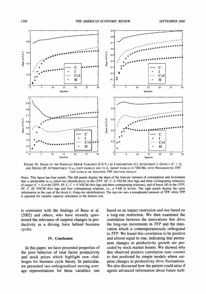
In order to evaluate the importance of this phenomenon in business cycles, Figure 10 reports the variance decompositions for consumption (C), investment (I), output (C + I), and hours worked (H) for the e2 and eZ shocks retrieved from the system based on either the adjusted or unadjusted measure of TFP. In order to calculate the variance decomposition for output and investment, we replaced hours worked in the four-variable VAR by investment or output. The impulse responses associated with these two latter exercises are not reported since they look similar to those in Figure 9.

The variance decompositions in Figure 10 indicate that 62, and similarly e1, explain a substantial fraction of fluctuations at business cycle frequencies. In effect, given the interpretation of this shock as reflecting news about technological innovations, the variance decomposition results suggest that news shocks may be a major source of business cycle fluctuations, even if surprise changes in productivity may not be. Let us note that the second part of this observation

Percent

deviation

Percent

deviation

Percent

deviation

Percent

deviation

Percent

deviation

Percent

deviation

Percent

deviation

Percent

deviation


1

0.8

0.6

0.4

0.2

0 0 5 10 15 20 25 30

Quarters

C I C+I H

0.9

0.8

0.7

0.6

0.5

0.4

0.3

0.2

0.1

0 0 5 10 15 20 25 30

Quarters

C I C+I H

0.9

0.8

0.7

0.6

0.5

0.4

0.3

0.2

0.1 0 5 10 15 20 25 30

Quarters

C I C+I H

0.8

0.6

0.4

0.2

0 0 5 10 15 20 25 30

Quarters

C I C+I H

FIGURE 10. SHARE OF THE FORECAST ERROR VARIANCE (F.E.V.) OF CONSUMPTION (C), INVESTMENT I, OUTPUT (C + I),

AND HOURS (H) ATTRIBUTABLE TO 62 (LEFT PANELS) AND TO a1 (RIGHT PANELS) IN VECMs, WITH NONADJUSTED TFP

(TOP PANELS) OR ADJUSTED TFP (BOTTOM PANELS)

Notes: This figure has four panels. The left panels display the share of the forecast variance of consumption and investment that is attributable to e2 (short-run identification) in the (TFP, SP, C, I) VECM (five lags and three cointegrating relations), of output (C + I) in the (TFP, SP, C, C + I) VECM (five lags and three cointegrating relations), and of hours (H) in the (TFP, SP, C, H) VECM (five lags and four cointegrating relations, i.e., a VAR in levels). The right panels display the same information in the case of the shock O (long-run identification). The top row uses a nonadjusted measure of TFP, while TFP is adjusted for variable capacity utilization in the bottom row.

is consistent with the findings of Basu et al. (2002) and others, who have recently ques- tioned the relevance of surprise changes in productivity as a driving force behind business cycles.

IV. Conclusion

In this paper, we have presented properties of the joint behavior of total factor productivity and stock prices which highlight new chal- lenges for business cycle theory. In particular, we presented two orthogonalized moving average representations for these variables: one

based on an impact restriction and one based on a long-run restriction. We then examined the correlation between the innovations that drive the long-run movements in TFP and the innovation which is contemporaneously orthogonal to TFP. We found this correlation to be positive and almost equal to one, indicating that permanent changes in productivity growth are pre- ceded by stock market booms. We showed why this observed positive correlation runs counter to that predicted by simple models where surprise changes in productivity drive fluctuations. We also discussed how the pattern could arise if agents advanced information about future tech-

Share

of F.E.V.

Share

of F.E.V.

Share

of F.E.V.

Share

of F.E.V.


nological opportunities. The results suggest that changes in technological opportunities may be central to business cycle fluctuations, even if surprise changes in productivity are not. Hence, these observations highlight the potential fruitful- ness of reexamining the manner in which productivity growth is modelled in business cycle analysis. In particular, the type of model that is needed to explain the observations is one where agents recognize changes in technological opportunities well in advance of their effect on productivity, and where the recognition itself leads to a boom in both consumption and investment, which precedes the growth in productivity.

REFERENCES

Basu, Susanto; Fernald, John and Kimball, Miles. "Are Technology Improvements Contrac- tionary?" National Bureau of Economic Re- search, Inc., NBER Working Papers: No. 10592, 2004.

Beaudry, Paul and Portier, Franck. "Stock Prices, News and Economic Fluctuations." National Bureau of Economic Research, Inc., NBER Working Papers: No. 10548, 2004.

Benhabib, Jess and Farmer, Roger E. A. "Inde- terminacy and Sunspots in Macroeconom- ics," in John B. Taylor and Michael Woodford, eds., Handbook ofmacroeconom- ics. Vol. 1A. Amsterdam: Elsevier Science, North-Holland, 1999, pp. 387-448.

Blanchard, Olivier Jean and Quah, Danny. "The Dynamic Effects of Aggregate Demand and Supply Disturbances." American Economic Review, 1989, 79(4), pp. 655-73.

Chao, John C. and Phillips, Peter C. B. "Model Selection in Partially Nonstationary Vector Autoregressive Processes with Reduced Rank Structure." Journal of Econometrics, 1999, 91(2), pp. 227-71.

Christiano, Lawrence J.; Eichenbaum, Martin and Vigfusson, Robert. "What Happens after a Technology Shock?" U.S. Federal Reserve Board, International Finance Discussion Pa- pers: No. 768, 2003.

Doan, Thomas J. RATS manual. Evanston, IL: Estima, 1992.

Fama, Eugene F. "Stock Returns, Expected Re- turns, and Real Activity." Journal of Fi- nance, 1990, 45(4), pp. 1089-1108.

Gali, Jordi. "Technology, Employment, and the Business Cycle: Do Technology Shocks Ex- plain Aggregate Fluctuations?" American Economic Review, 1999, 89(1), pp. 249-71.

Hamilton, James D. Time series analysis. Prince- ton: Princeton University Press, 1994.

Johansen, Sbren. "Determination of Cointegrat- ing Rank in the Presence of a Linear Trend." Oxford Bulletin of Economics and Statistics, 1992, 54(3), pp. 383-97.

Keynes, John Maynard. The general theory of employment, interest and money. London: Macmillan, 1936.

Nyblom, Jukka and Harvey, Andrew. "Tests of Common Stochastic Trends." Econometric Theory, 2000, 16(2), pp. 176-99.

Pigou, Arthur C. Industrial fluctuations. Lon- don: Macmillan, 1927.

Schwert, G. William. "Stock Returns and Real Activity: A Century of Evidence." Journal of Finance, 1990, 45(4), pp. 1237-57.

stock prices, news, and economic fluctuations - (macro)economics

Documents