stock markets volatility and international...

Journal of Business Studies Quarterly 2010, Vol. 1, No. 4, pp. 21-34 ISSN 2152-1034

Stock Markets Volatility and International Diversification

Mohamed Imen Gallali, Business School of Tunis, Tunisia Besma Kilani, Business School of Tunis, Tunisia

Abstract

During the last decades, the financial markets volatility concept attracted the attention of the theorists and the experts in the field of finance, especially for the internationally diversified wallets. In this article, we used an asymmetric dynamic conditional correlation (DCC-GARCH (1.1)) model following the approach of Engle (2002), to test if the volatility of individual market or their relative volatility causes the changing in correlation. The study focuses on the seven developed (G7) countries over the period 01/01/2000:31/12/2008. The results indicate that there is a significant effect of individual volatilities and correlations between the US market and the other markets and that individual volatility of these markets has an impact on the increase in correlations between the G7 countries.

Key words: International diversification, volatility, financial markets and DCC-GARCH. Introduction

During the last two decades, financial markets globalisation provided investors with so many investment opportunities. Likewise, the increasing establishment of foreign investment barriers helped outline an international portfolio diversification scheme, as it offers investors the possibility to improve their portfolio earnings. Gupta and Donleavy (2009) defined international diversification as « a risk management technique » that combines several foreign investments in one portfolio. Such diversification has uncontested advantages attributes to the low correlations between domestic financial markets. According to many new studies, international diversification has potential advantages compared to a domestic one (Chiou et al. 2009).

Financial theory made it clear that portfolio international diversification has been the best way to increase portfolio earnings and reduce global risk, notably systematic risk. The total risk for a given portfolio consists of two components:

- The stock-based risk known as diversifiable or specific risk.

- The domestic stock market-based risk known as systematic risk.

© Mohamed Imen Gallali and Besma Kilani

22

The first risk may be reduced by a domestic diversification plan, whereas the systematic risk can be attenuated only with an international diversification plan.

International diversification is essentially based on the degree of interdependence between different stock market indexes. As such, testing the effect of volatility as an explanatory factor is a compelling task (Gupta et al. (2009). Volatility is often considered as a risk to investors. This financial markets volatility has often attracted the attention of finance theorists and practitioners because of its importance in evaluating stocks and managing risk, notably in the case of internationally-diversified portfolios. In this regard, investors should take heed from two major volatility dimensions; non-constancy and persistence. Recently, several recent studies have focused attention on this concept proposing a number of volatility evaluation models. We can mention the ARCH model developed by Engle (1982) and the GARCH model proposed by Boullerslev (1986). However, worth mentioning is the inability of these models to integrate the asymmetry of volatility hypothesis. To solve for this inconvenience, Nelson (1991) proposes the Exponential GARCH model (EGARCH), while Rabemananjara and Zakoian (1993) propose the Threshold GARCH model (TGARCH). Financial theory assumes that covariances between stocks play a crucial role. Nevertheless, these univariate models fail to take into account this covariance aspect, hence the emergence of more developed models like Engle’s Dynamic Conditional Correlation GARCH model (DCC-GARCH(1.1)) (Engle, 2002) .

In this paper, we will examine international diversification on a sample of seven developed countries (the United States of America, France, Germany, Italy, Canada, UK and Japan) (G7 countries) over the 01/01/2000 to 31/12/2008 period. This paper is organised as follows. The second section discusses the different theoretical and empirical proposals about the advantages and limits of international diversification. The third section presents the methodology, whereas the fourth section presents data analysis and the obtained results. The last section proposes the conclusions. Review of Literature

A given stock’s volatility measures the rates up and down movements over a given period of time. The more these variations are intense in a short time horizon, the higher volatility is. Poon and Granger (2002) insist that there is an incomplete appreciation of the differences between volatility and risk. With the relative success of the conditional heteroskedasticity models (ARCH/GARCH) in modelling volatility of economic series and notably financial series, two extensions have been noted as relevant. On the one hand, the use of high-frequency data has often been equated with a unitary root-based approach to study conditional volatility, where the IGARCH model (Engle et al. 1986) fits. On the other hand, there is the use of fractional integration parameters notably within the FIGARCH models (Baillie, Bollerslev and Mikkelsen, 1996). The IGARCH (p, q), proposed by Engle and Bollerslev (1986), is a process integrated into variance which implies persistence of shocks (an infinite persistence of the impulsions response function). Indeed, Baillie (1996) assumes that financial series’ volatility correlations are particularly consistent with a hyperbolic decrease, i.e. they play a mediating behaviour between an exponential decrease in GARCH models, which are less persistent, and the absence of a decrease induced by IGARCH models (Lespagnol C. and Teiletche J. (2005)). An IGARCH model produces the asymptotic stationarity of a GARCH (p.q) model. In contrast to an IGARCH model, the Fractionally Integrated GARCH (FIGARCH) model proposed by Baillie, Bollerslev and Mikkelsen (1996) offers a direct measure of persistence

Journal of Business Studies Quarterly 2010, Vol. 1, No. 4, pp. 21-34

©JBSQ 2010 23

through fractional integration parameters. Moreover, the effect of a volatility shock is reduced to a hyperbolic component in time, which allows better identifying long-term volatility. The fractional difference parameter (d) allows the indirect measurement of long-term persistence of volatility. Laurent and Beine (2000) evaluated the persistence of change rates’ volatility using a FIGARCH model over the 1980-1996 period. They found out that long-term persistence of shocks diminished when the currency’s volatility degree remained stable during the whole period. Volatility asymmetry points to a negative correlation between returns and conditional variance of the following period. These negative returns are associated to an increase in conditional volatility. Asai M. and McAleer M. (2008) believe that negative shocks affect volatility more than positive and similar shocks. Worth noting is that during stock markets shocks, we notice an outstanding presence of volatility asymmetry, because with a rise in volatility comes a substantial decrease in stock prices. Despite the success of ARCH/GARCH models, they are unable to incorporate the asymmetry hypothesis. To solve for this, Nelson (1991) proposed the EGARCH model and few years later Rabemananjara and Zakoian (1993) proposed the TGARCH model. Volatility transfer may be due to stock markets sensitivity to countries’ macroeconomic similarities or to a common shock. Shocks transfers should be taken seriously as they are likely to transfer quickly and significantly affect both developed and emerging markets. These latter are likely to react more significantly to a shock over the American market than to a shock in an emerging market (Bekaert et al. (2003)). Parket and Song (2000) tested volatility contagion during the 1997-1998 crisis between Asian change markets, applying a GARCH model. Their results indicated that the crisis effect on Indonesia and Thailand is transmitted to the Korean change market, yet the Korean crisis did not affect the two countries. According to Bekaert, Harvey and Ng (2005), the introduction of the bivariate GARCH model may resolve this problem. Bekaert, Harvey and Ng (2005) illustrate that the relationships between domestic stock markets tend to be stronger enough during crises than during stable periods. In their study, Semedo and Malik (2007) applied these equations using Bollerslev model under the returns and variance variation hypothesis and the correlation constancy assumption. Then, they chose a dynamic correlation case. The results indicate that correlation dynamics across markets point to an increase in interdependencies between geographically close markets. Tse (2000) and Solnik and Longin (2001) have long criticised correlation constancy statement and insist that this hypothesis is very restrictive. Falvin and Panopoulou (2009) examined volatility across stable and unstable periods applying the switching volatility model and using Garvelle et al.’s methodology (2006). The authors believe that the switching model is advantageous to other previous techniques, knowing that the country under shock was not included in the analysis. This model has been used to test the stability of common shocks transfer between each country pair. The obtained results show that, on the one hand, returns during stable periods are significantly positive whereas in unstable periods returns are negative. On the other hand, the model allowed for detecting that common shocks are characterized in average by a high volatility layout. Against these results, it seems that international diversification remains a good option even in times of crises. Moreover, American investors are able to reduce risk if they integrate foreign stocks in their portfolios. Ólan T. H. (2009) examined, during the January 1980 to August 2007 period, the effect of volatility on the earnings of portfolios, studying the relationship between these earnings and short-term interest rates in stable and unstable periods. The author studied volatility using the


24

switching EGARCH model. In this model, the first class of data consists of high earnings and low variance, while the second class consists of low earnings and high variance. For the first class, the author found out a conditional volatility persistent and asymmetrical to stocks’ earnings innovations. As for the second class, the author found out that conditional variance is asymmetrical, yet persistence of volatility shocks are absent through time. In so far as portfolio management is concerned, stocks covariances play a crucial role in investors’ decision-making process regarding placement strategies. Nevertheless, we notice that univariate models fail to take into account this aspect. Likewise, multivariate ARCH and GARCH models are not easy to implement. Other models are developed among which is Engle’s (2002) where correlations are dynamic. Gupta and Donleavy (2009) believe that following market integration, diversification advantages vanish although investors have become more and more aware of the importance of this strategy in increasing profits and reducing risk. The authors have examined correlations change between the Australian and emerging markets during the 1988-2005 period, testing volatility as factor causing this change. The authors applied the asymmetric Engle’s Dynamic Conditional Correlation GARCH model or DCC-GARCH (1.1) model following Engle’s approach (2002). The obtained results illustrate that correlations between the studied markets change during time and that this variation is affected by individual volatility of each market and the Australian market volatility and those of the emerging markets. The advantages of international diversification depend on the correlations between domestic and foreign stocks. An accurate assessment of these correlations help investors better select the indexes which are the most performing so as to retain an efficient portfolio. Methodology

In this section, we propose the dynamic conditional correlations asymmetric model. The reduced form of the autoregressive model is written as follows:

A(L) yt = c + εt with εt follows N(0, Ht) for t = 1, 2,.............T (1)

Where: A(L) is the polynomial lag and εt = [ε1t, ε2t] is a residuals vector retained from estimating the autoregressive model for each variable.

The DCC-GARCH (1.1) asymmetric model may be easily reproduced by writing the variance-covariance matrix (H) in a way Ht = Dt Rt Dt.

Where: Dt = a diagonal { tih } : the diagonal matrix of standard deviations variable in time.

The elements of D are generated using a GARCH (p, q) model that can be written as follows:

∑ ∑= =

−− ++=Pi

p

Qi

qqitiqpitpiiit hwh

1 1

2 βεα 2,1=∀i (2)

With:

α : lagged error squares,

β : lagged conditional variance,

ω : Asymmetric term. The (α , β ,ω ) parameters of the DCC model are estimated using a maximum likelihood estimation.


©JBSQ 2010 25

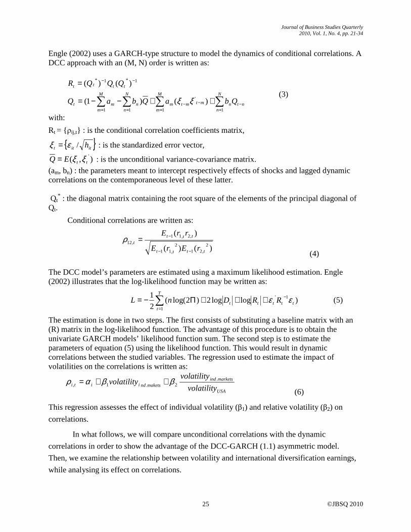
Engle (2002) uses a GARCH-type structure to model the dynamics of conditional correlations. A DCC approach with an (M, N) order is written as:

∑ ∑∑∑

= =−−−

==

−−

++−−=

=M

m

N

nntnmtmtm

N

nn

M

mmt

tttt

QbaQbaQ

QQQR

1 1

'

11

1*1*

)()1(

)()(

ξξ (3)

with:

Rt = {ρij,t} : is the conditional correlation coefficients matrix,

{ }ititt h/εξ = : is the standardized error vector,

),( 'ttEQ ξξ= : is the unconditional variance-covariance matrix.

(am, bn) : the parameters meant to intercept respectively effects of shocks and lagged dynamic correlations on the contemporaneous level of these latter. Qt

* : the diagonal matrix containing the root square of the elements of the principal diagonal of Qt.

Conditional correlations are written as:

)()(

)(2

,212

,11

,2,11,12

tttt

tttt

rErE

rrE

−−

−=ρ

(4) The DCC model’s parameters are estimated using a maximum likelihood estimation. Engle (2002) illustrates that the log-likelihood function may be written as:

)loglog2)2log((

2

1 1'

1tttt

T

tt RRDnL εε −

=

+++Π−= ∑ (5)

The estimation is done in two steps. The first consists of substituting a baseline matrix with an (R) matrix in the log-likelihood function. The advantage of this procedure is to obtain the univariate GARCH models’ likelihood function sum. The second step is to estimate the parameters of equation (5) using the likelihood function. This would result in dynamic correlations between the studied variables. The regression used to estimate the impact of volatilities on the correlations is written as:

USA

marketsindmaketsndiiti volatility

volatilityvolatility .

2.1, ββαρ ++= (6)

This regression assesses the effect of individual volatility (β1) and relative volatility (β2) on

correlations.

In what follows, we will compare unconditional correlations with the dynamic

correlations in order to show the advantage of the DCC-GARCH (1.1) asymmetric model.

Then, we examine the relationship between volatility and international diversification earnings,

while analysing its effect on correlations.


26

Empirical Evidence

Data The study focuses on the G7 countries: the United States of America, France, Germany, Italy,

Canada, UK and Japan, as they represent 80% to 85% of the international stock market capitalisation. The data for these markets are the stock markets indexes expressed in terms of local currency and the change rates against the US dollar. They are weekly data over the 01/01/2000 - 31/12/2008 period, totalling 3290 observations. These indexes are expressed in US dollar to avoid problems arising from change rate variations1. Earnings are expressed in US dollar in excess of a 30-day bond’s earnings. This approach assumes that investors are open to risk or, in the same way, change prices are supposedly null.

Descriptive Statistics and the Preliminary Analysis Results of earnings analysis, reported in Table 1 below, show that France has the lowest positive mean (0.05%), while Canada has negative values (-0.0013) during the study period, earnings maximum value is that of France (30%) whereas for the rest of the sample earnings values are around 20%. Table 1: Descriptive Statistics of stock markets indices’ weekly earnings in US Dollar

Earnings volatility analysis shows that standard deviations are higher for the US market (2.7%)

which represents the lowest deviation risk. This can be partially explained by the fact that

earnings are converted in US dollar. Consequently, unconditional variance does not include, for

the US market, change rate risk. With reference to Table 2, we notice that most of the domestic

inter-market correlations are inferior to 0.5 and are sometimes negative for the

Germany/Canada and Italy/Canada pairs. Moreover, correlation coefficients between the US

market and the other markets are low, except for France and the UK (0.605 and 0.604). This

suggests that international diversification presents a significant risk-reduction opportunity.

Such an information may be used to form a diversified portfolio, by combining indices with

low positive correlations. 1 The stock market rates are taken from the “Yahoo Finance » on-line data base. Change rates are taken from the

« Oanda » on-line data base. For the weekly observations, the website offers the opening, closing, highest and lowest

rates. We chose for the context of our study the closing rates.

USA France Canada UK Germany Japan Italy Mean(%) 0. 12 0.05 -0. 13 0. 12 0. 16 0. 15 0. 12

Medium(%) -0. 1 -0. 13 -0. 4 -0. 1 -0. 29 0. 046 -0. 19

Max(%) 20.1 30 22.3 25.1 25.6 25.5 25.7

Min(%) -11.35

-13,65 -36.3 -10.7 -15.7 -17.1 -15.7

Standard Deviations(%)

2.7 3.4 3.5 2.8 3.7 3.4 3.3


©JBSQ 2010 27

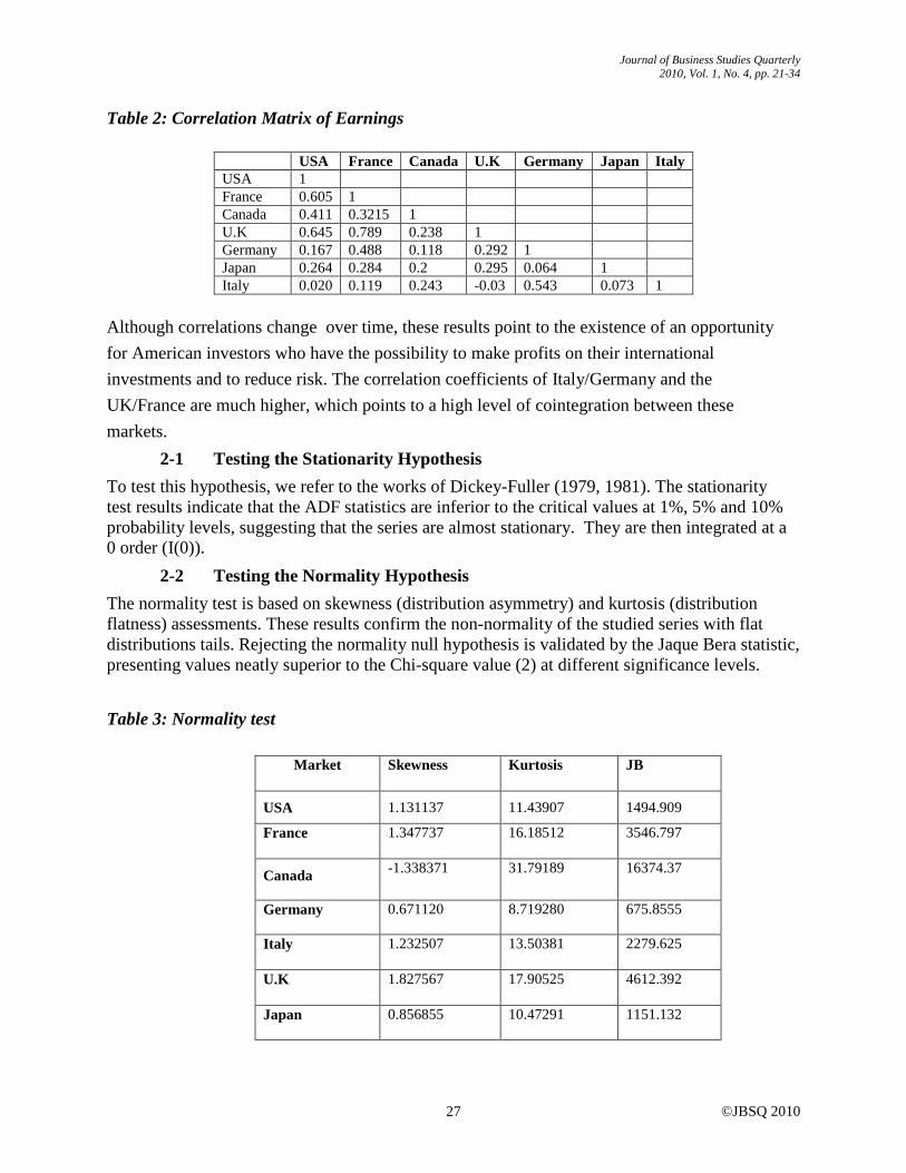
Table 2: Correlation Matrix of Earnings

Although correlations change over time, these results point to the existence of an opportunity

for American investors who have the possibility to make profits on their international

investments and to reduce risk. The correlation coefficients of Italy/Germany and the

UK/France are much higher, which points to a high level of cointegration between these

markets.

2-1 Testing the Stationarity Hypothesis

To test this hypothesis, we refer to the works of Dickey-Fuller (1979, 1981). The stationarity test results indicate that the ADF statistics are inferior to the critical values at 1%, 5% and 10% probability levels, suggesting that the series are almost stationary. They are then integrated at a 0 order (I(0)).

2-2 Testing the Normality Hypothesis

The normality test is based on skewness (distribution asymmetry) and kurtosis (distribution flatness) assessments. These results confirm the non-normality of the studied series with flat distributions tails. Rejecting the normality null hypothesis is validated by the Jaque Bera statistic, presenting values neatly superior to the Chi-square value (2) at different significance levels.

Table 3: Normality test

USA France Canada U.K Germany Japan Italy USA 1 France 0.605 1 Canada 0.411 0.3215 1 U.K 0.645 0.789 0.238 1 Germany 0.167 0.488 0.118 0.292 1 Japan 0.264 0.284 0.2 0.295 0.064 1 Italy 0.020 0.119 0.243 -0.03 0.543 0.073 1

Market Skewness Kurtosis JB

USA 1.131137 11.43907 1494.909

France 1.347737 16.18512 3546.797

Canada -1.338371 31.79189 16374.37

Germany 0.671120 8.719280 675.8555

Italy 1.232507 13.50381 2279.625

U.K 1.827567 17.90525 4612.392

Japan 0.856855 10.47291 1151.132


28

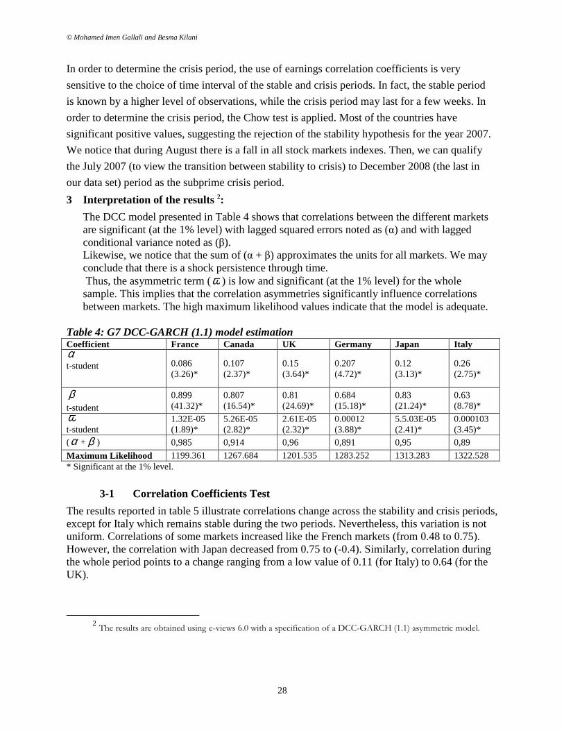
In order to determine the crisis period, the use of earnings correlation coefficients is very

sensitive to the choice of time interval of the stable and crisis periods. In fact, the stable period

is known by a higher level of observations, while the crisis period may last for a few weeks. In

order to determine the crisis period, the Chow test is applied. Most of the countries have

significant positive values, suggesting the rejection of the stability hypothesis for the year 2007.

We notice that during August there is a fall in all stock markets indexes. Then, we can qualify

the July 2007 (to view the transition between stability to crisis) to December 2008 (the last in

our data set) period as the subprime crisis period.

3 Interpretation of the results 2:

The DCC model presented in Table 4 shows that correlations between the different markets are significant (at the 1% level) with lagged squared errors noted as (α) and with lagged conditional variance noted as (β). Likewise, we notice that the sum of (α + β) approximates the units for all markets. We may conclude that there is a shock persistence through time. Thus, the asymmetric term (ω ) is low and significant (at the 1% level) for the whole sample. This implies that the correlation asymmetries significantly influence correlations between markets. The high maximum likelihood values indicate that the model is adequate.

Table 4: G7 DCC-GARCH (1.1) model estimation Coefficient France Canada UK Germany Japan Italy α t-student 0.086

(3.26)* 0.107 (2.37)*

0.15 (3.64)*

0.207 (4.72)*

0.12 (3.13)*

0.26 (2.75)*

β

t-student 0.899 (41.32)*

0.807 (16.54)*

0.81 (24.69)*

0.684 (15.18)*

0.83 (21.24)*

0.63 (8.78)*

ω t-student

1.32E-05 (1.89)*

5.26E-05 (2.82)*

2.61E-05 (2.32)*

0.00012 (3.88)*

5.5.03E-05 (2.41)*

0.000103 (3.45)*

(α + β ) 0,985 0,914 0,96 0,891 0,95 0,89

Maximum Likelihood 1199.361 1267.684 1201.535 1283.252 1313.283 1322.528 * Significant at the 1% level.

3-1 Correlation Coefficients Test

The results reported in table 5 illustrate correlations change across the stability and crisis periods, except for Italy which remains stable during the two periods. Nevertheless, this variation is not uniform. Correlations of some markets increased like the French markets (from 0.48 to 0.75). However, the correlation with Japan decreased from 0.75 to (-0.4). Similarly, correlation during the whole period points to a change ranging from a low value of 0.11 (for Italy) to 0.64 (for the UK).

2 The results are obtained using e-views 6.0 with a specification of a DCC-GARCH (1.1) asymmetric model.

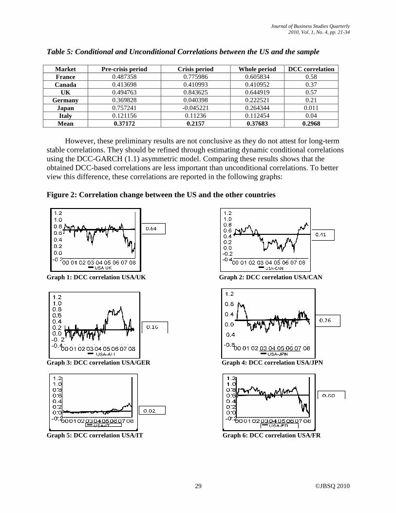
Table 5: Conditional and Unconditional Correlations between the US and the sample

Market Pre-crisis period France 0.487358 Canada 0.413698

UK 0.494763 Germany 0.369828

Japan 0.757241 Italy 0.121156 Mean 0.37172

However, these preliminary results are not conclusive as they do not attest for long

stable correlations. They should be refined through estimating dynamic conditional correlations using the DCC-GARCH (1.1) asymmetric model. Comparing these results shows that the obtained DCC-based correlations are less important thview this difference, these correlations are reported in the following graphs: Figure 2: Correlation change between the US and the other countries

Graph 1: DCC correlation USA/UK

Graph 3: DCC correlation USA/GER

Graph 5: DCC correlation USA/IT

Journal of Business Studies Quarterly2010

29

Unconditional Correlations between the US and the sample

Crisis period Whole period DCC correlation0.775986 0.605834 0.410993 0.410952 0.843625 0.644919 0.040398 0.222521 -0.045221 0.264344 0.11236 0.112454 0.2157 0.37683

However, these preliminary results are not conclusive as they do not attest for longcorrelations. They should be refined through estimating dynamic conditional correlations

GARCH (1.1) asymmetric model. Comparing these results shows that the based correlations are less important than unconditional correlations.

view this difference, these correlations are reported in the following graphs:

orrelation change between the US and the other countries

DCC correlation USA/UK Graph 2: DCC correlation USA/CAN

DCC correlation USA/GER Graph 4: DCC correlation USA

DCC correlation USA/IT Graph 6: DCC correlation USA/FR

Business Studies Quarterly 2010, Vol. 1, No. 4, pp. 21-34

©JBSQ 2010

Unconditional Correlations between the US and the sample

DCC correlation 0.58 0.37 0.57 0.21 0.011 0.04

0.2968

However, these preliminary results are not conclusive as they do not attest for long-term correlations. They should be refined through estimating dynamic conditional correlations

GARCH (1.1) asymmetric model. Comparing these results shows that the an unconditional correlations. To better

Graph 2: DCC correlation USA/CAN

DCC correlation USA/JPN

DCC correlation USA/FR


30

Conditional correlation is plotted in the graph as a straight line in order to view the comparison between unconditional correlations and correlations variable in time. American indexes correlations with Italy float around the period with no clear pattern, whereas those with Germany increased during the same period. The effect of the subprime crisis (2007) on these countries may be viewed on the graphs as extreme fluctuations during crisis period. This assessment of correlations may help investors take optimal decisions to insure higher profitability of an internationally diversified portfolio. Then, they should take into account France’s and Germany’s high correlations with the US.

Comparing these results with those obtained through a constant correlation, we notice the absence of a high correlation for Germany, which points to the reliability of the DCC-GARCH (1.1) asymmetric model vis-a-vis the unconditional correlations approach. These results are consistent with the proposals of Tse (2000) and Solnik and Longin (2001), Bera and Kim (2001), who criticised constant correlation in time.

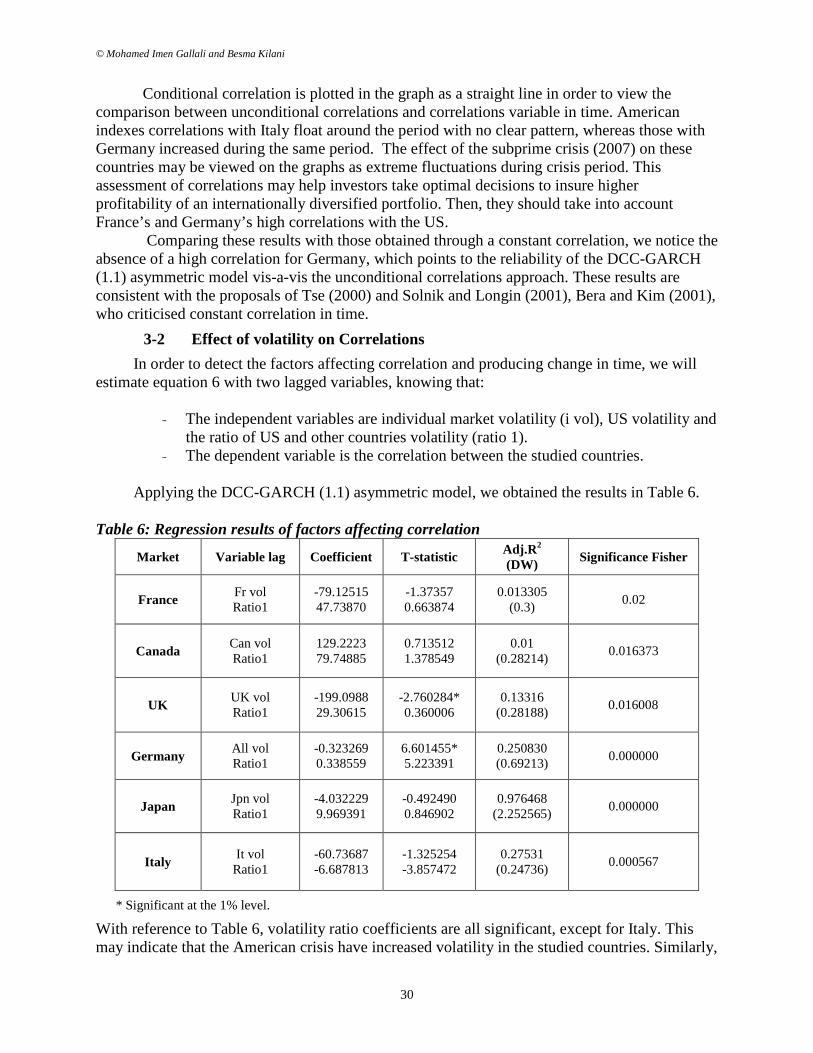
3-2 Effect of volatility on Correlations

In order to detect the factors affecting correlation and producing change in time, we will estimate equation 6 with two lagged variables, knowing that:

- The independent variables are individual market volatility (i vol), US volatility and the ratio of US and other countries volatility (ratio 1).

- The dependent variable is the correlation between the studied countries.

Applying the DCC-GARCH (1.1) asymmetric model, we obtained the results in Table 6. Table 6: Regression results of factors affecting correlation

Market Variable lag Coefficient T-statistic Adj.R2

(DW) Significance Fisher

France Fr vol Ratio1

-79.12515 47.73870

-1.37357 0.663874

0.013305 (0.3)

0.02

Canada Can vol Ratio1

129.2223 79.74885

0.713512 1.378549

0.01 (0.28214)

0.016373

UK UK vol Ratio1

-199.0988 29.30615

-2.760284* 0.360006

0.13316 (0.28188)

0.016008

Germany All vol Ratio1

-0.323269 0.338559

6.601455* 5.223391

0.250830 (0.69213)

0.000000

Japan Jpn vol Ratio1

-4.032229 9.969391

-0.492490 0.846902

0.976468 (2.252565)

0.000000

Italy It vol Ratio1

-60.73687 -6.687813

-1.325254 -3.857472

0.27531 (0.24736)

0.000567

* Significant at the 1% level.

With reference to Table 6, volatility ratio coefficients are all significant, except for Italy. This may indicate that the American crisis have increased volatility in the studied countries. Similarly,


©JBSQ 2010 31

we notice that the UK, Germany, Japan and Italy have Adj.R2 coefficients superior to 0.1, suggesting that a portion of correlation variations are explained by the independent variables (individual volatility and the ratio of volatility between markets). The Fisher statistics are significant for all the countries, indicating that correlation fluctuations in time are explained by the independent variables. In summary, the obtained results suggest that the studied markets’ volatility has an important and significant impact on the US vs other markets correlations.

Conclusion

Correlations between financial markets play a determinant role in an international diversification strategy. For this reason, an accurate evaluation of this factor helps investors to form an optimal portfolio. Recent portfolio management research focused on the factors affecting correlations change in time such as volatility.

The application of the DCC-GARCH (1.1) asymmetric model on the G7 countries as a sample allowed us to view a high volatility between the US and France, the UK, and Germany, and low volatility with Italy, Canada, and Japan. This correlation variation needs an analysis of the factors affecting this change. The obtained results, using a regression analysis of the correlations between the studied markets and individual volatility of each market and relative volatility (volatilities ratios) point to the existence of a reverse relationship between correlations and individual volatility. Indeed, when this volatility diminishes, correlations between markets increase for all countries, except for the Canadian market. These results indicate that there is a significant impact of individual volatilities and correlations between the US market and the other markets.

The DCC-GARCH (1.1) asymmetric model helped us compare unconditional and dynamic correlations. The correlation graphs point to, beyond for France and the UK, the existence of a high correlation between the US and Germany. Consequently, the test seems to be more reliable as we could not detect a high correlation for this pair of countries applying a constant correlation method. Moreover, we showed that individual volatility of the studied markets has an impact on the increase in correlations between the G7 countries.

International diversification strategy brings more profits while insuring a reduction in risk. Nevertheless, during these last two decades, financial markets have been characterized by an increasing integration, which caused correlations between markets to increase and international diversification profits to decrease. This may partially explain investors’ tendency to opt for emerging markets which are characterized by high earnings and a low correlation with developed stock markets. These markets are often segmented and they may insure a superior return rate for a given risk level. References

Ackermann J. (2008). The subprime crisis and its consequence. Journal of Financial Stability,

vol. 4, pp: 329–337.

Angelidis T., & Tessaromatis N. (2009). Idiosyncratic risk matters! A regime switching

approach. International Review of Economics and Finance, vol. 18, pp: 132–141.

Asai M., & McAleer M. (2008). Asymmetric Multivariate Stochastic Volatility. Econometric

Reviews, vol.25, No. 2, pp: 453 – 473.


32

Baillie, R.T., Bollerslev, T., & Mikkelsen, H.O. (1996). Fractionally Integrated Generalized

Autoregressive Conditional Heteroskedasticity. Journal of Econometrics, Vol. 74, pp: 3-30.

Beine M., & Laurent S. (2000). La persistance des chocs de volatilité sur le marché des changes

s'est-elle modifiée depuis le début des années 1980? Revue économique, Vol. 51, No. 3, pp.

703-711.

Beine, M., Laurent, S., & Lecourt, C. (1999). Accounting for conditional leptokurtosis and

closing days effects in FIGARCH models of daily exchange rates. Communication présentée

au 6ième Workshop of Financial Modelling,Lille, Janvier.

Bergin, P. (2008). Understanding international portfolio diversification and turnover rates. Int.

Fin. Markets, Inst. and Money, vol. 18, pp: 191–206.

Bollerslev, T. (1986). Generalized Autoregressive Conditional Heteroskedasticity. Journal of

Econometric, vol. 31, pp: 307-327.

Bollerslev, T., & Mikkelsen, H. (1996). Modeling and pricing long memory in stock market

volatility, Journal of Econometrics, Vol. 73, pp: 151-184.

Bollerslev, T., & Engle, R.F., (1993). Common Persistence in Conditional Variances,

Econometrica, 61, 167-186.

Chin Wen C. (2008). Time-varying volatility in Malaysian stock exchange: An empirical study

using multiple-volatility-shift fractionally integrated model. The Journal of Finance, Vol.

387, pp: 889–898.

Chiou W. (2009). Benefits of international diversification with investment constraints: An over-

time perspective. Journal of Multi. Finance Management, Vol. 19 pp: 93–110.

Dos Santosa, M. (2008). Does corporate international diversification destroy value? Evidence

from cross-border mergers and acquisitions. Journal of Banking & Finance, Vol. 32, PP:

2716-2724.

Engle, R. (2002). Dynamic Conditional Correlation – A Simple Class of Multivariate GARCH.

Engle, R. F. (1982). Autoregressive Conditional Heteroskedasticity with Estimates of the

Variance of UK Inflation, Econometrica, Vol. 50, pp: 987–1008.

Flavin T., & Panopoulou, E. (2009). On the robustness of international portfolio diversification

benefits to regime-switching volatility. Int. Fin. Markets, Inst. and Money, vol. 19, pp: 140–

156.

Froot, K.A. (1993). Risk Management : Coordinating Corporate Investment and Financing

Policies. Journal of Finance, vol. 48, pp: 1629-1648.

Gastineau, G. (1995). The Currency Hedging Decision: A Search for Synthesis in Asset

Allocation. Financial Analysts Journal, pp: 8-17.

Gupta R., & Donleavy, G.D. (2009). Benefits of diversifying investments into emerging markets

with time-varying correlations. Journal of Multinational Financial Management, 19, 160-177.


©JBSQ 2010 33

Gupta, R., & Mollik, A. (2008). Volatility, Time Varying Correlation and International Portfolio

Diversification: An Empirical Study of Australia and Emerging Markets. International

Research Journal of Finance and Economics, Vol.18, pp: 1450-2887.

Hamilton J. D. (1994). Time Series Analysis, Princeton University Press: New Jersey.

Henry, Ó. (2009). Regime switching in the relationship between equity returns and short-term

interest rates in the UK. Journal of Banking & Finance, vol. 33 pp: 405–414.

Iwaisako, T. (2002). Does International Diversification Really Diversify Risks? Journal of the

Japanese and International Economies, vol. 16, pp: 109–134.

Izquierdo, A., & Lafuente J. (2004). International transmission of stock exchange volatility:

Empirical evidence from the Asian crisis. Global Finance Journal, vol.15, pp: 125– 137.

Jermann, U. (2002). International portfolio diversification and endogenous labor supply choice.

European Economic Review, vol.46, pp: 507–522.

Kizys, R., & Pierdzioch, C. (2009). Changes in the international co-movement of stock returns

and asymmetric macroeconomic shocks. Int. Fin. Markets, Inst. and Money, Vol.19, pp: 289–

305.

Krishnan, C. (2008). Correlation Risk. Journal of Empirical Finance, Vol.53, No.98, pp: 82-83.

Lespagnol, C., & Teiletche, J. ( 2005). La dynamique de la volatilité à très haute fréquence des

taux longs.

Longin, F., & Bruno S. (2001). Extreme Correlation of International Equity Markets. Journal of

Finance, 56(2): 649–676.

McMillan, D., & Ruiz, I. (2007). Volatility persistence, long memory and time-varying

unconditional mean: Evidence from 10 equity indices. The Quarterly Review of Economics

and Finance, Vol. 49, pp: 578-595

Meyer, T. (2003). The persistence of international diversification benefits before and during the

Asian crisis. Global Finance Journal, vol.14, pp: 217–242.

Nautz, D. (2008). Volatility transmission in the European money market. North American

Journal of Economics and Finance, vol. 19, pp: 23–39.

Nelson, D. (1991). Cconditional Heteroskedasticity in Asset Returns: A New Approch.

Econometrica, Vol. 59, No. 2, pp: 347-370;

Olibe, K. (2008). Systematic risk and international diversification: An empirical perspective.

International Review of Financial Analysis, Vol. 17, pp: 681-698.

Phengpisa, C. (2004). Increasing input information, realistically measuring potential

diversification gains from international portfolio investments. Global Finance Journal,

vol.15, pp: 197- 217.

Phylaktis, K., & Ravazzolo F. (2005). Stock market linkages in emerging markets: implications


34

for international portfolio diversification. Int. Fin. Markets, Inst. and Money, vol. 15, pp: 91–

106.

Poon, S., & Granger, R. (2002). Forecasting Volatility in Financial Markets: A Review.

Rzepkowski, B. (2001). Pouvoir prédictif de la volatilité implicite dans le prix des options de

change. Économie et Prévision, vol. 2, No. 148, pp: 71 – 97.

Salehi, M. (2003). U.S. multinationals and the home bias puzzle: an empirical analysis. Global

Finance Journal, vol. 14, pp: 303– 318.

Schwebach, R.(2002). The impact of financial crises on international diversification. Global

Finance Journal, vol. 13, pp: 147–161.

Smith, K. (2008). The dynamics among G7 government bond and equity markets and the

implications for international capital market diversification. Research in International

Business and Finance, vol. 22, pp: 222–245.

Solnik, B. (1996). International Market Correlation and Volatility. Financial Analyst Journal,

vol. 52, pp: 17-34.

Solnik B. (1999). Correlation structure of international equity markets during extremely

volatility periods. Livre.

Tse, Y.K. (2000). A Test for Constant Correlations in a Multivariate GARCH model. Journal of

Econometrics, vol.13 pp: 107-127.

Vinh, X. (2009). International financial integration in Asian bond markets. Research in

International Business and Finance, Vol. 23, pp: 90-106

Wu, G. (2001). The Determinants of asymmetric volatility. The Review of Financial Studies,

Vol.14, No.3, pp: 837.

Zakoian, J. M. (1994). Threshold heteroskedastic models. Journal of Economic Dynamics and

Control, Vol.18, pp: 931–995

stock markets volatility and international...

Documents