stochastic simulation in multi-scale modeling
TRANSCRIPT
Stochastic simulation in multi-scale modeling
Lori Graham-Brady
Associate ProfessorDepartment of Civil Engineering
560.700 – Applications of Science-Based Coupling of Models
September 29-October 1, 2008

GOAL: QUANTIFICATION OF STRUCTURAL GOAL: QUANTIFICATION OF STRUCTURAL RELIABILITY (e.g., probability of failure)RELIABILITY (e.g., probability of failure)
Load variability important: studied extensivelyLoad variability important: studied extensively
Material/geometric variability: studied lessMaterial/geometric variability: studied less
Need for multiNeed for multi--scale analysis that incorporates uncertaintyscale analysis that incorporates uncertainty
OBJECTIVE AND GENERAL OUTLINEOBJECTIVE AND GENERAL OUTLINE

GOAL: QUANTIFICATION OF STRUCTURAL GOAL: QUANTIFICATION OF STRUCTURAL RELIABILITY (e.g., probability of failure)RELIABILITY (e.g., probability of failure)
Load variability important: studied extensivelyLoad variability important: studied extensively
Material/geometric variability: studied lessMaterial/geometric variability: studied less
Need for multiNeed for multi--scale analysis that incorporates uncertaintyscale analysis that incorporates uncertainty
•• (Cursory) overview of multi(Cursory) overview of multi--scale approachesscale approaches
•• Motivation for probabilistic analysisMotivation for probabilistic analysis
•• Simulation of stochastic microstructureSimulation of stochastic microstructure
•• Simulation of material properties (elastic, inelastic, Simulation of material properties (elastic, inelastic, brittle strength)brittle strength)
OBJECTIVE AND GENERAL OUTLINEOBJECTIVE AND GENERAL OUTLINE

Why multi-scale?• Failure of macro-scale
structures often initiates/propagates at micro- or nano-scale
• Full-scale models with explicit small-scale features are infeasible
• Multi-scale models incorporate small-scale information into large-scale models

Multi-scale approaches (deterministic)
Concurrent multi-scale models (e.g., Robbins, Fish, Ghosh, Liu): coupling of scales in a single model
•Many assumptions regarding boundaries between scales
•Assumptions regarding very low temperature, etc.
•Assumes that information is available at all scales –deterministic
•Use when necessary –challenging!

Multi-scale approaches (deterministic)
Hierarchical or information-passing models: calculate effective behavior and pass to large scale models
•Decouples scales: no feedback between scales
•Makes use of single-scale results (experimental, computational, analytical)
•In place for a long time (e.g., homogenization)
•Well suited for probabilistic models
σf, Em,…
σy, E,…
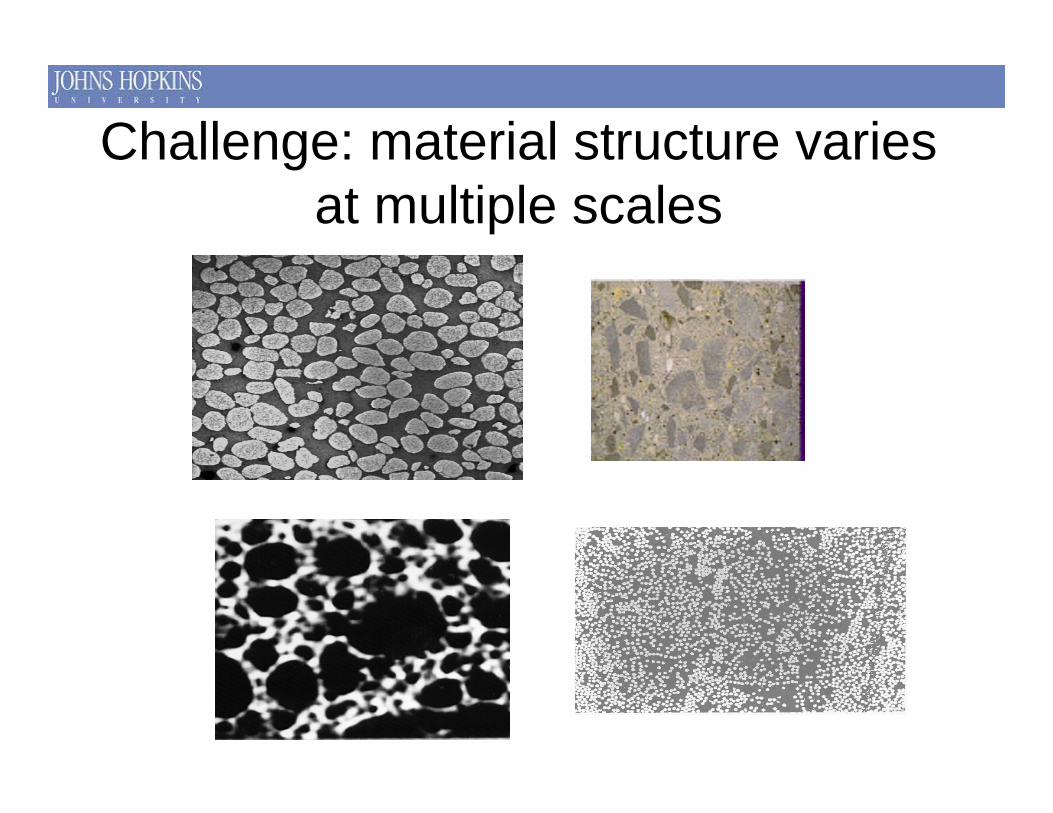
Challenge: material structure varies at multiple scales
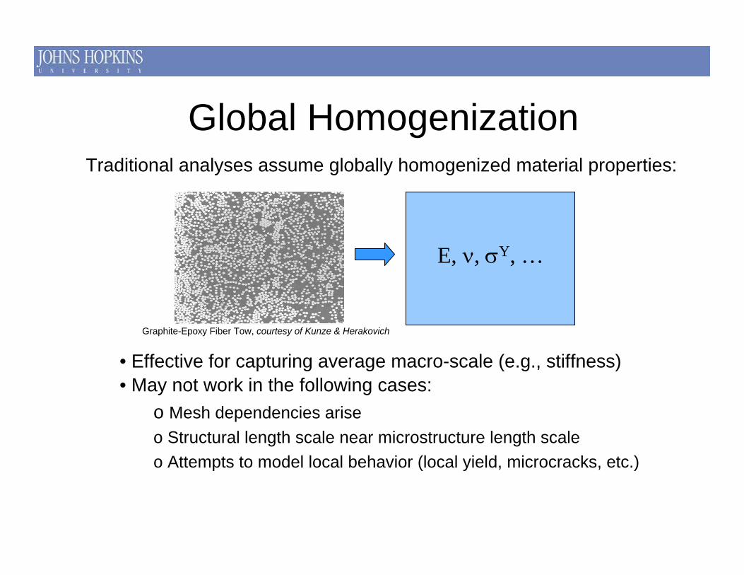
Global HomogenizationTraditional analyses assume globally homogenized material properties:
• Effective for capturing average macro-scale (e.g., stiffness)• May not work in the following cases:
o Mesh dependencies ariseo Structural length scale near microstructure length scaleo Attempts to model local behavior (local yield, microcracks, etc.)
Graphite-Epoxy Fiber Tow, courtesy of Kunze & Herakovich
E, ν, σY, …

Mesh dependencyThe assumption of homogeneous material properties in modeling localized failure leads to mesh dependencies
•Observed in models of shear bands – results explicitly connected to mesh size rather than physics of the problem
Medyanik et al, JMPS 2007

Small length scalesP
P
Stiffness of small-scale “beams” vary significantly due to crystal orientation of grains

Inelastic behavior dependent on local effectsInelastic behavior dependent on local effectsLocal concentrations obscured by homogenizationLocal concentrations obscured by homogenization
Models of local behavior

Why probabilistic?Importance of spatially varying behavior highlightedRandom material properties lead to random behavior -
predicting scatter is critical to reliability estimates
failure
Probability density function of strength
Higher mean & higher variance lead to more likely failure than lower mean & lower variance

Why probabilistic?• Predicting scatter is critical to survivability
estimates• Deterministic models may not capture typical
behavior, even when it’s not random
Cracking/shear bands: assumptions on initiation sites –can be idiosyncratic
Yielding: simultaneous yielding at all locations

Why probabilistic?• Predicting scatter is critical to survivability
estimates• Deterministic models may not capture typical
behavior• Localized loadings make small-scale material
fluctuations important

Simple example – cantilever beamCalculate variance of displacement at x=L/2, when stiffness EI(x) varies randomly over length of beam.
• Random spatial variability can be significant to structural response!

How do probabilistic hierarchical models work?
• Deterministic model passes continuum-based parameter(s) to the next larger scale
Deterministic: predict continuum-based conditions for onset of shear bands, fracture, other quantity of interest (eg, failure stress)
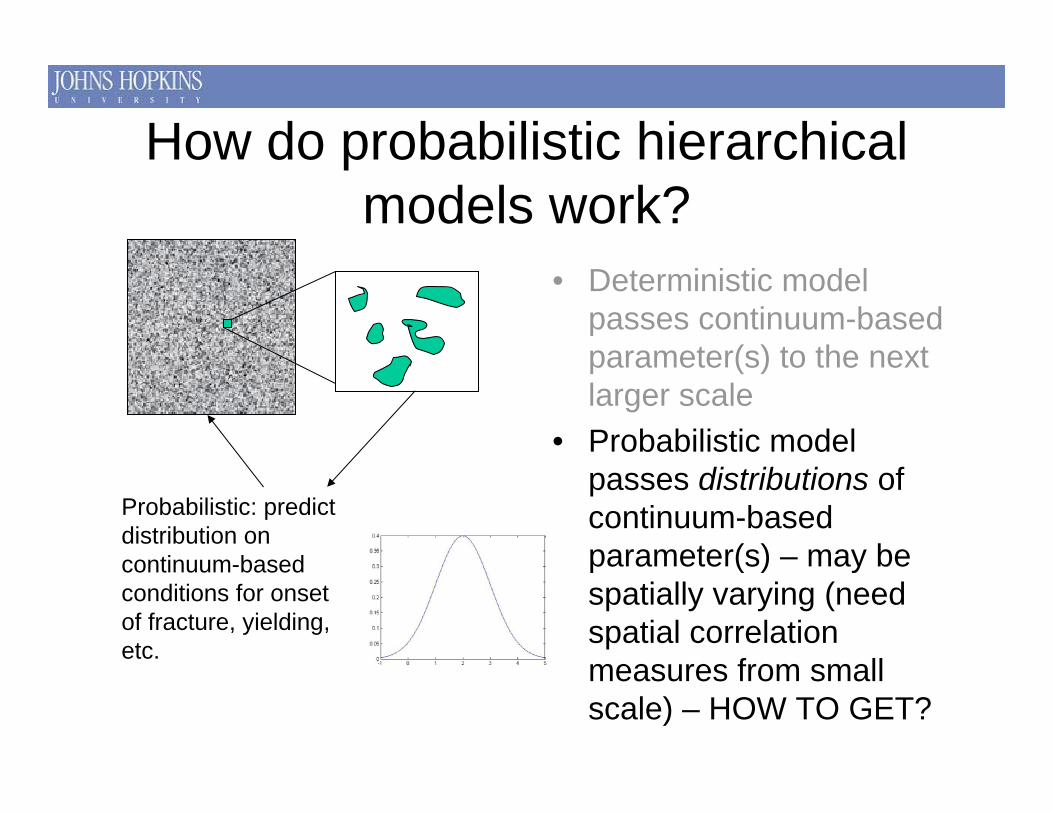
How do probabilistic hierarchical models work?
• Deterministic model passes continuum-based parameter(s) to the next larger scale
• Probabilistic model passes distributions of continuum-based parameter(s) – may be spatially varying (need spatial correlation measures from small scale) – HOW TO GET?
Probabilistic: predict distribution on continuum-based conditions for onset of fracture, yielding, etc.

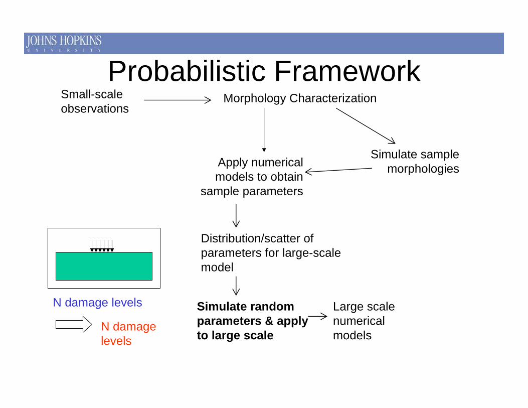
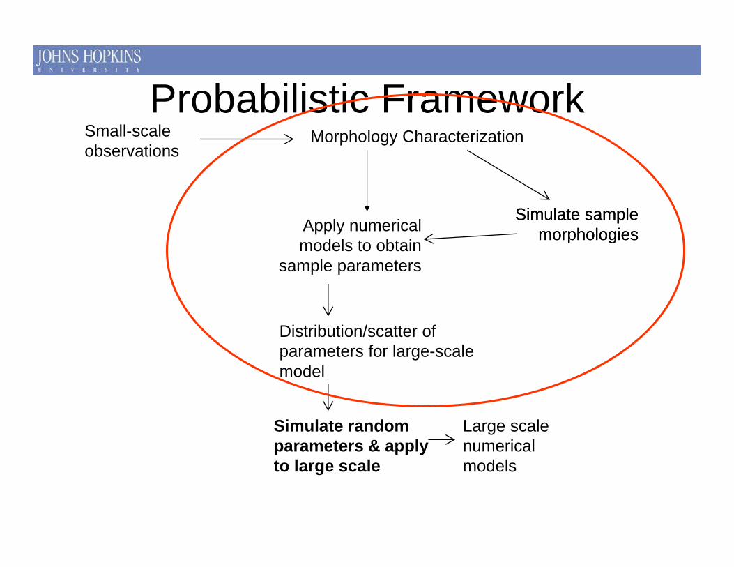
Probabilistic Framework
Large scale numerical models
Small-scale observations
Identify scatter in large scale results
Proper prediction of failure
Microstructure varies randomly from location to location

Distribution/scatter of parameters for large-scale model
Large scale numerical models
Probabilistic FrameworkSmall-scale observations

Distribution/scatter of parameters for large-scale model
Experimental results
Largedatasets available
Large scale numerical models
Wouldn’t it be nice to have this for all materials?!
Probabilistic FrameworkSmall-scale observations
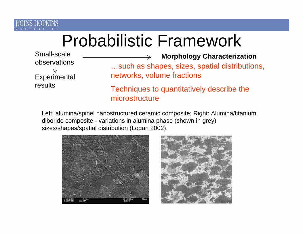
Morphology Characterization…such as shapes, sizes, spatial distributions, networks, volume fractions
Techniques to quantitatively describe the microstructure
Left: alumina/spinel nanostructured ceramic composite; Right: Alumina/titanium diboride composite - variations in alumina phase (shown in grey) sizes/shapes/spatial distribution (Logan 2002).
Experimental results
Probabilistic FrameworkSmall-scale observations
Distribution/scatter of parameters for large-scale
model
Simulate sample morphologies
Apply numerical models to obtain
sample parameters
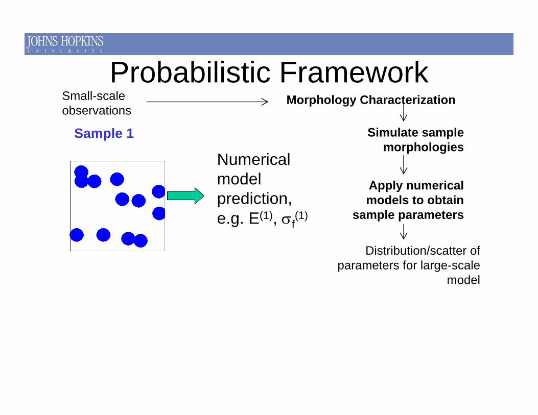
Numerical model prediction, e.g. E(1), σf
(1)
Sample 1
Morphology Characterization
Probabilistic FrameworkSmall-scale observations
Distribution/scatter of parameters for large-scale
model
Simulate sample morphologies
Apply numerical models to obtain
sample parameters
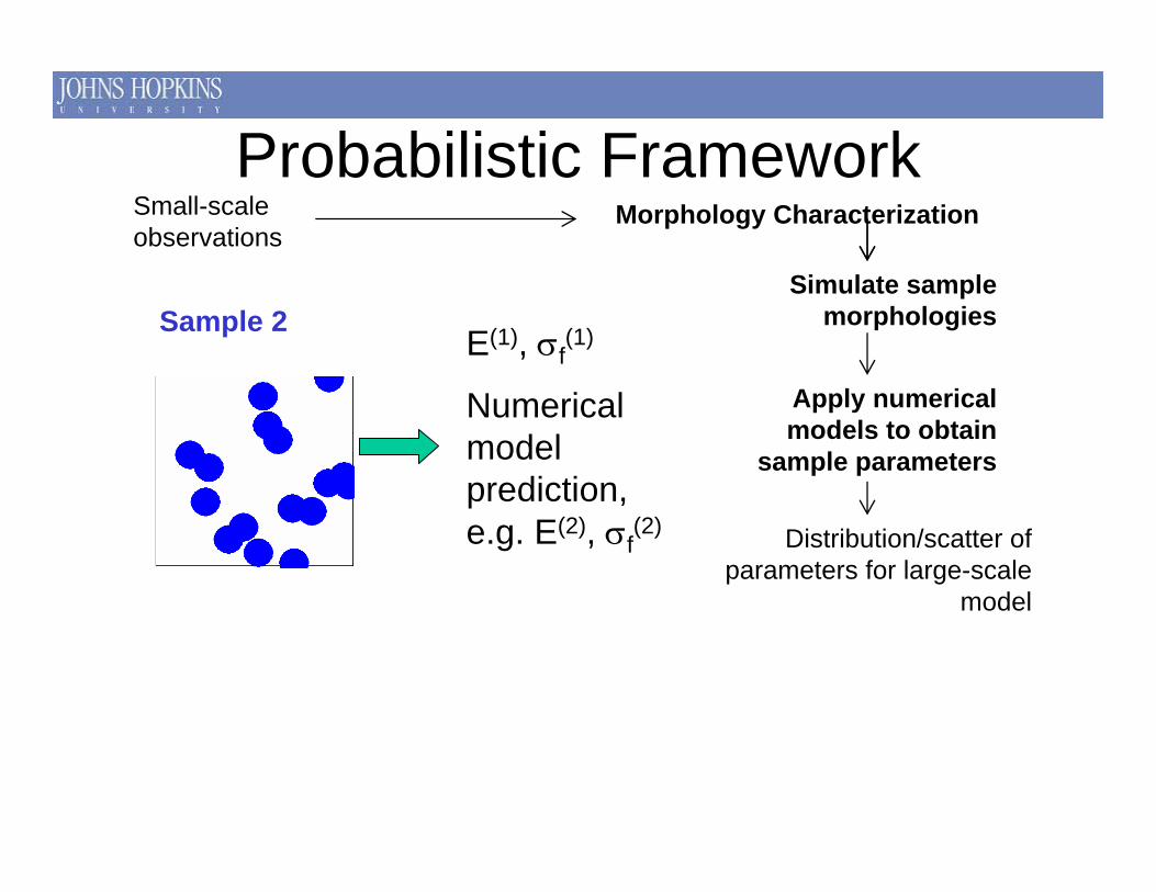
E(1), σf(1)
Numerical model prediction, e.g. E(2), σf
(2)
Sample 2
Morphology Characterization
Probabilistic FrameworkSmall-scale observations

Distribution/scatter of parameters for large-scale
model
Simulate sample morphologies
Apply numerical models to obtain
sample parameters
E(1), σf(1)
E(2), σf(2)
E(N), σf(N)
Sample N
Morphology Characterization
Probabilistic FrameworkSmall-scale observations

Distribution/scatter of parameters for large-scale
model
Simulate sample morphologies
Apply numerical models to obtain
sample parameters
E(1), σf(1)
E(2), σf(2)
E(N), σf(N)
Morphology Characterization
Probabilistic FrameworkSmall-scale observations

Distribution/scatter of parameters for large-scale model
Simulate sample morphologiesApply numerical
models to obtain sample parameters
Morphology Characterization
Probabilistic FrameworkSmall-scale observations
Microstructure Local E(x,y)

Distribution/scatter of parameters for large-scale model
Simulate sample morphologiesApply numerical
models to obtain sample parameters
Simulate random parameters & apply to large scale
Large scale numerical models
Morphology Characterization
Probabilistic FrameworkSmall-scale observations
Generate Sample 1 of material properties (depends on (x,y))
Damage D1
Distribution/scatter of parameters for large-scale model
Simulate sample morphologiesApply numerical
models to obtain sample parameters
Simulate random parameters & apply to large scale
Large scale numerical models
Morphology Characterization
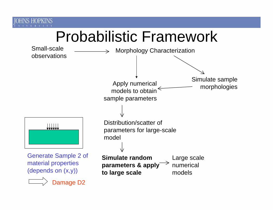
Probabilistic FrameworkSmall-scale observations
Generate Sample 2 of material properties (depends on (x,y))
Damage D2
Distribution/scatter of parameters for large-scale model
Apply numerical models to obtain
sample parameters
Simulate random parameters & apply to large scale
Large scale numerical models
N damage levels
Probabilistic Framework
N damage levels
Simulate sample morphologies
Morphology CharacterizationSmall-scale observations

Distribution/scatter of parameters for large-scale model
Simulate sample morphologiesApply numerical
models to obtain sample parameters
Simulate random parameters & apply to large scale
Large scale numerical models
N damage levels
Estimate of scatter in performance
Probabilistic Framework
Simulate sample morphologies
Morphology CharacterizationSmall-scale observations
Distribution/scatter of parameters for large-scale model
Simulate sample morphologiesApply numerical
models to obtain sample parameters
Simulate random parameters & apply to large scale
Large scale numerical models
Probabilistic Framework
Simulate sample morphologies
Morphology CharacterizationSmall-scale observations
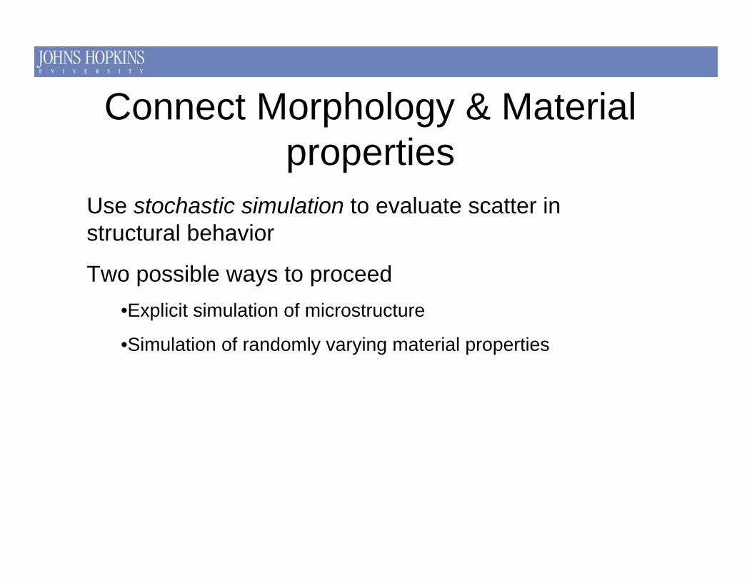
Use stochastic simulation to evaluate scatter in structural behavior
Two possible ways to proceed•Explicit simulation of microstructure
•Simulation of randomly varying material properties
Connect Morphology & Material properties

Use stochastic simulation to evaluate scatter in structural behavior
Two possible ways to proceed•Explicit simulation of microstructure
•Simulation of randomly varying material properties
Connect Morphology & Material properties

Some microstructures are fairly straightforward to generate –special cases
Spherical/Cylindrical inclusions, randomly distributed with some level of clustering
Voronoi tessellation, assuming uniform grain growth
Microstructural Simulation
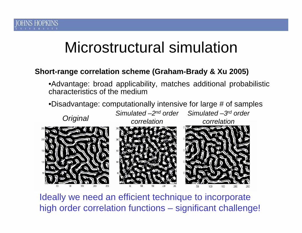
Short-range correlation scheme (Graham-Brady & Xu 2005)•Advantage: broad applicability, matches additional probabilisticcharacteristics of the medium •Disadvantage: computationally intensive for large # of samples
OriginalSimulated –3rd order
correlation
Ideally we need an efficient technique to incorporate high order correlation functions – significant challenge!
Simulated –2nd order correlation
Microstructural simulation

Put each simulated microstructure into a finite element model (or other computational mechanics models) of the structureCalculate statistics on the response of interest…Model is simple to envision, but simulation not so simple
OriginalSimulated –3rd order
correlationSimulated –2nd order
correlation
Using microstructural simulation

Use stochastic simulation to evaluate scatter in structural behavior
Two possible ways to proceed•Explicit simulation of microstructure
•Simulation of randomly varying material properties
Connect Morphology & Material properties
Use stochastic simulation to evaluate scatter in structural behavior
Two possible ways to proceed•Explicit simulation of microstructure
•Simulation of randomly varying material properties
Calls for statistics of randomly varying material properties: probability density function, correlation functions
Connect Morphology & Material properties

Collect E at every point (x,y) – place in a bin
Draw a histogram from the bin
Fit a probability density function to the histogram
Probability density function
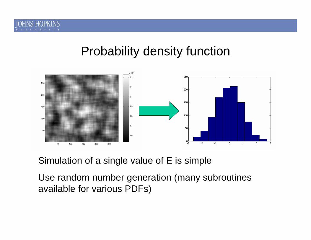
Simulation of a single value of E is simple
Use random number generation (many subroutines available for various PDFs)
Probability density function

Probability density function
Simulation of a many values of E is simple, if none of the values are correlated!

Correlation function ρ(τx, τy) measures the correlation between values of E at a distance τx and τy apart
Points close together well-correlated (ρ near 1)
Points far apart poorly correlation (ρ near 0)
Correlation function

Use stochastic simulation to evaluate scatter in structural behavior
Two possible ways to proceed•Explicit simulation of microstructure
•Simulation of randomly varying material properties
Calls for statistics of randomly varying material properties: probability density function, correlation functions
NEED A SAMPLE SET OF RANDOMLY VARYING MATERIAL PROPERTIES!
Connect Morphology & Material properties

Microstructure Local Material Properties (Exx(x,y))
2 specific approaches considered here:
•Moving-window homogenization (elastoplasticcomposite)
•Local flaw distributions (brittle material)
Link microstructure to material properties

•Pixelized image with distinct phases
•Coupled with a micromechanical homogenization method
•Overlapping windows
•Larger window size leads to more homogenization
Moving-window homogenization

•Pixelized image with distinct phases
•Coupled with a micromechanical homogenization method
•Overlapping windows
•Larger window size leads to more homogenization
Moving-window homogenization

• Rule of Mixtures: Assume stiffness is volume average of stiffness, or flexibility is volume average of flexibility –different results unless volume is very large!
• Mori-Tanaka: Represent each window as a single fiber with volume that satisfies volume fraction
vf=4/9=.444 vf=4/9=.444
Both approaches ignore configuration of phases
Micromechanics
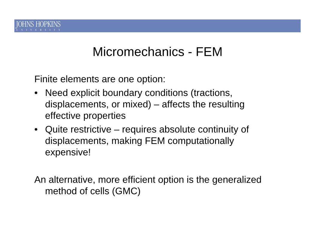
Finite elements are one option:• Need explicit boundary conditions (tractions,
displacements, or mixed) – affects the resulting effective properties
• Quite restrictive – requires absolute continuity of displacements, making FEM computationally expensive!
An alternative, more efficient option is the generalized method of cells (GMC)
Micromechanics - FEM

Strain in Composite
Strain in Subcell
Stress in Subcell
Stress in Composite
Input Constitutive
Relation
Strain Concentration
Volumetric Averaging
Conditions/Assumptions:•Periodic•Continuous Fiber
•Traction Continuity•Displacement Continuity
Paley and Aboudi, 1992
Micromechanics - GMC

Strain in Composite
Strain in Subcell
Stress in Subcell
Stress in Composite
Input Constitutive
Relation
Strain Concentration
Volumetric Averaging
Conditions/Assumptions:•Periodic•Continuous Fiber
•Traction Continuity•Displacement Continuity
Paley and Aboudi, 1992
Micromechanics - GMC
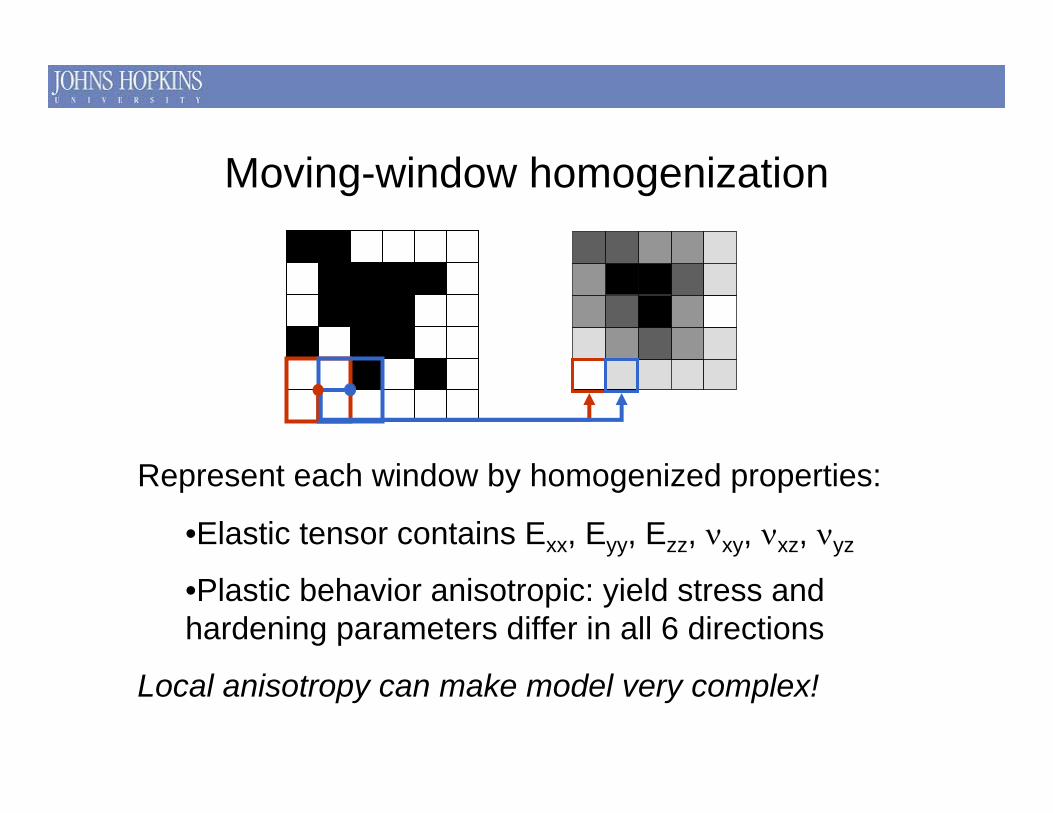
Moving-window homogenization
Represent each window by homogenized properties:
•Elastic tensor contains Exx, Eyy, Ezz, νxy, νxz, νyz
•Plastic behavior anisotropic: yield stress and hardening parameters differ in all 6 directions
Local anisotropy can make model very complex!

Sample
Ematrix=91 GPa
Efiber=414 GPa
φfiber=25%
νmatrix=νfiber=0.2
Moving-window Mori Tanaka
Moving-window FEMMoving-window GMC
Effect of micromechanics model on local Exx(x,y) (minimal)

Sample
20%x20% Window2.5%x2.5% Window
How to pick?
Ultimately depends on scale that has most effect on response of interest
Effect of window size on Exx(x,y) – significant!

Microstructure digitized into rectangular pixels – direct application to FEM model leads to artificial stress concentrations.
Single circular fiber in matrix leads to a maximum tensile stress of 1.26 (relative to average tensile stress of 1)
Model based on resolution above leads to stress of 1.62 – error!
Example: stress around fiber

In the elastic range, a window size of approximately the inclusion size gives the best solution for maximum stress (true for any resolution)
Window size – single fiber

Local Material Properties (Exx(x,y)) Response to loading (stress)
Locally, stress is affected by variations in elastic modulus – higher than predictions from model with fully homogenized properties
Provide material properties to FEM model

Stresses, using FE model and material property fields from a 5%x5% window size
σyy σxx
p(x)=1 MPa
1.62
Example – Local stress distribution

Distribution/scatter of parameters for large-scale model
Simulate sample morphologiesApply numerical
models to obtain sample parameters
Simulate random parameters & apply to large scale
Large scale numerical models
Probabilistic Framework
Simulate sample morphologies
Morphology CharacterizationSmall-scale observations

Exx(x,y) from given material microstructure (left)
Exx(x,y) generated by stochastic simulation (right)
Simulation of elastic properties
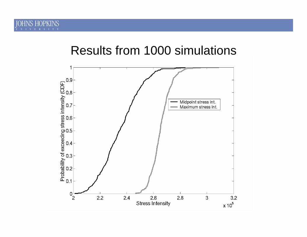
Results from 1000 simulations

Results from 1000 simulations
Homogenized prediction

Results from 1000 simulations
Design threshold

Distribution/scatter of parameters for large-scale model
Simulate sample morphologiesApply numerical
models to obtain sample parameters
Simulate random parameters & apply to large scale
Large scale numerical models
Probabilistic Framework
Simulate sample morphologies
Morphology CharacterizationSmall-scale observations

Microstructural observations
2 specific approaches considered here:
•Moving-window homogenization (elastoplastic material)
•Local flaw distributions (brittle material)
Link microstructure to material properties
Flaw density
Clustering of flaws
Flaw size distribution
Probability density function (PDF) of local strain-rate-dependent constitutive parameters

Strain rate dependence in brittle materials
Impact problems: stress waves serve to “localize” loads
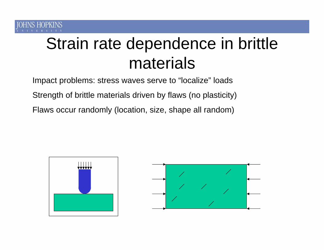
Strain rate dependence in brittle materials
Impact problems: stress waves serve to “localize” loads
Strength of brittle materials driven by flaws (no plasticity)
Flaws occur randomly (location, size, shape all random)
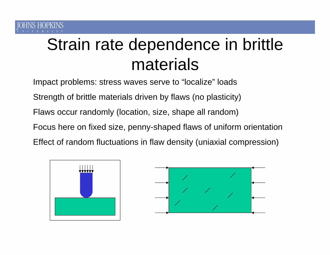
Strain rate dependence in brittle materials
Impact problems: stress waves serve to “localize” loads
Strength of brittle materials driven by flaws (no plasticity)
Flaws occur randomly (location, size, shape all random)
Focus here on fixed size, penny-shaped flaws of uniform orientation
Effect of random fluctuations in flaw density (uniaxial compression)

Mesh dependency in models of failure
The assumption of homogeneous material properties in modeling localized failure leads to mesh dependencies
•Brannon’s work shows improved mesh independency when strength is allowed to vary spatially
In FEM, each element has a different strength – varies randomly!

Mesh dependency in models of failure
The assumption of homogeneous material properties in modeling localized failure leads to mesh dependencies
•Brannon’s work shows improved mesh independency when strength is allowed to vary spatially
How to decide what are appropriate distributions of strength?
Shape of PDF of strength (Weibull)?
Mean/Variance of strength?

Mesh dependency in models of failure
The assumption of homogeneous material properties in modeling localized failure leads to mesh dependencies
•Brannon’s work shows improved mesh independency when strength is allowed to vary spatially
Mean/Variance of strength affected by:
Element size
Flaw density, clustering, flaw size distribution

Effect of element size on local flaw density
0 0.5 1 1.5 2 2.5
x 104
0
0.5
1
1.5
2
2.5
3
3.5
4x 10⁻³ PDF of flaws/unit volume for different area fractions of bulk
A=1x1A=.25x.25A=0.1x0.1A=.025x.025 Effect of
clustering?
large,small →→ σV
Assuming flaw locations are independent, then local flaw densityis Poisson-distributed
Bulk flaw density=104
flaws/unit volume

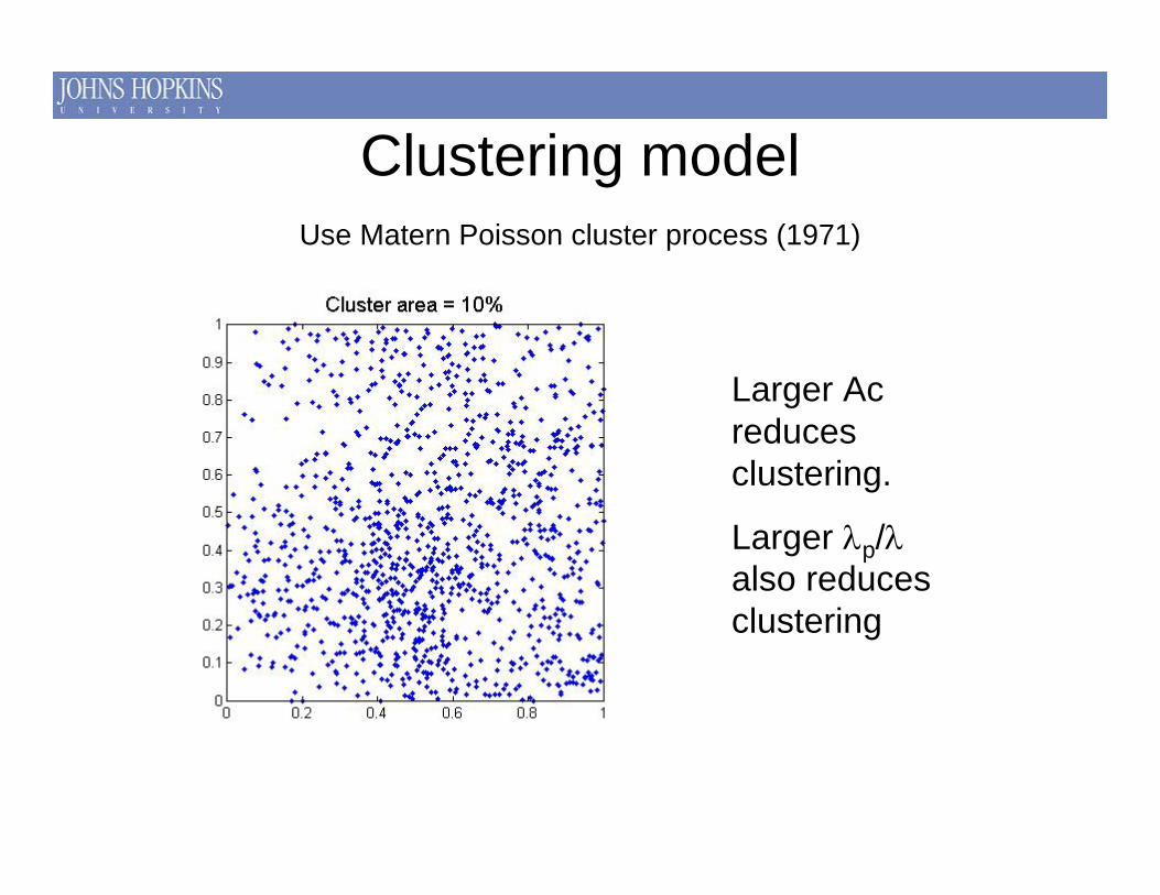
Clustering model
Generate N parent points (Poisson process with parameter λpA)
Use Matern Poisson cluster process (1971)
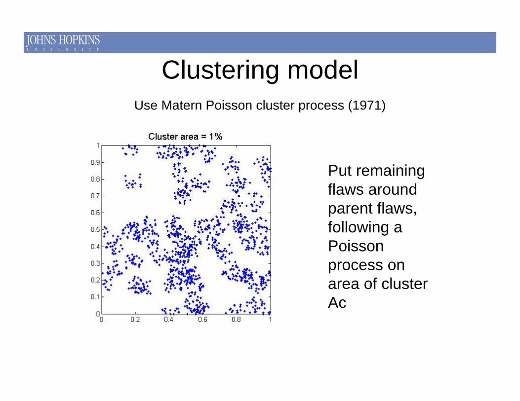
Clustering model
Put remaining flaws around parent flaws, following a Poisson process on area of cluster Ac
Use Matern Poisson cluster process (1971)
Clustering model
Larger Ac reduces clustering.
Larger λp/λalso reduces clustering
Use Matern Poisson cluster process (1971)

Clustering model
Diggle (1978) shows how to estimate λpand Ac for given microstructure using nearest neighbor distribution
Use Matern Poisson cluster process (1971)
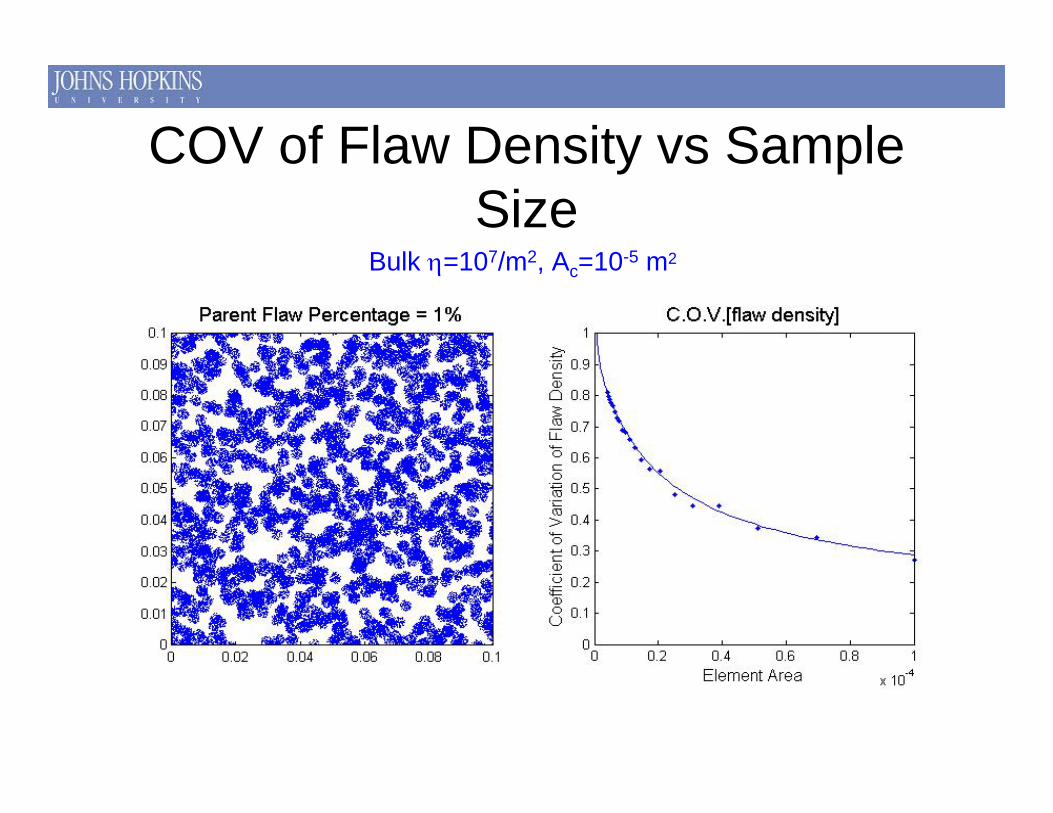
COV of Flaw Density vs Sample Size
Bulk η=107/m2, Ac=10-5 m2

COV of Flaw Density vs Sample Size
NOTE: COV is the standard deviation divided by the mean

COV of Flaw Density vs Sample Size
Bulk η=107/m2, Ac=10-5 m2

COV of Flaw Density vs Sample Size
Bulk η=107/m2, Ac=10-5 m2

COV of Flaw Density vs Sample Size
Bulk η=107/m2, Ac=10-5 m2

COV of Flaw Density vs Sample Size
Bulk η=107/m2, Ac=10-5 m2

COV of Flaw Density vs Sample Size
Bulk η=107/m2, Ac=10-5 m2

COV of Flaw Density vs Sample Size
Bulk η=107/m2, Ac=10-5 m2

COV of Flaw Density vs Sample Size
Bulk η=107/m2, Ac=10-5 m2

COV of Flaw Density vs Sample Size
Bulk η=107/m2, Ac=10-5 m2
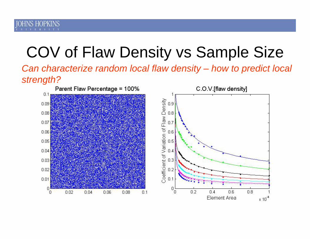
Can characterize random local flaw density – how to predict local strength?
COV of Flaw Density vs Sample Size

Microstructural observations for given element size, clustering level, average flaw density
Link microstructure to material properties
Mean & variance of flaw density
Flaw size distribution (deterministic for now)
Probability density function (PDF) of local strain-rate-dependent constitutive parameters – strength under uniaxial compression

Under compression, frictional sliding of flaws produce tension cracks at the tips
Cracks grow in direction of maximum compression, causing axial splitting
σ1
σ1
σ1
σ1
Ashby & Hallam, Acta met. 1986
Brittle failure under compression

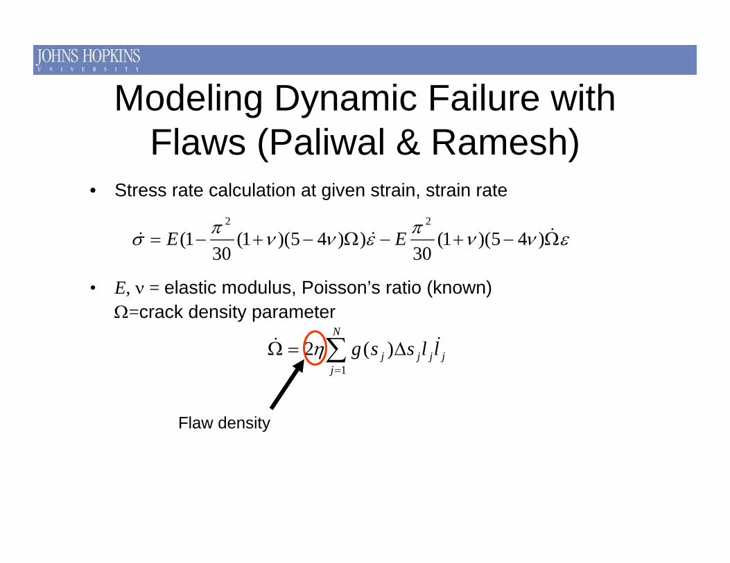
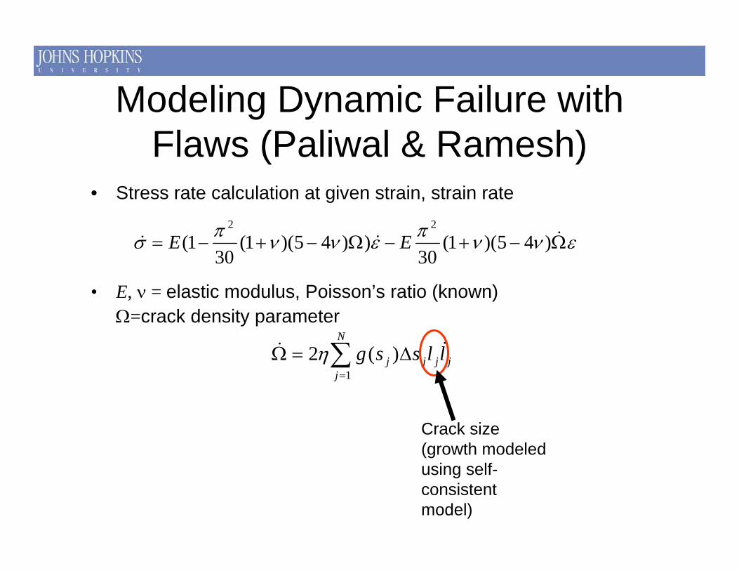
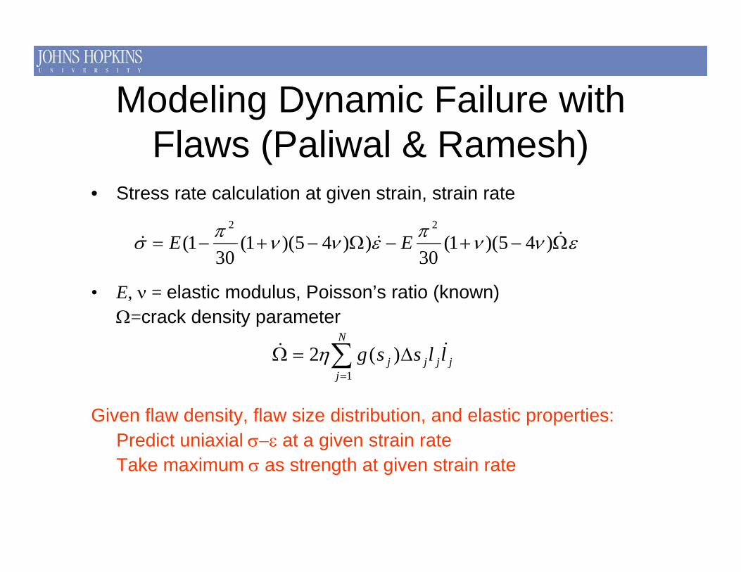
Modeling Dynamic Failure with Flaws (Paliwal & Ramesh)
• Stress rate calculation at given strain, strain rate
• E, ν = elastic modulus, Poisson’s ratio (known)Ω=crack density parameter
εννπεννπσ Ω−+−Ω−+−= &&& )45)(1(30
))45)(1(30
1(22
EE
jjj
N
jj llssg && Δ=Ω ∑
=
)(21
η
Modeling Dynamic Failure with Flaws (Paliwal & Ramesh)
• Stress rate calculation at given strain, strain rate
• E, ν = elastic modulus, Poisson’s ratio (known)Ω=crack density parameter
εννπεννπσ Ω−+−Ω−+−= &&& )45)(1(30
))45)(1(30
1(22
EE
jjj
N
jj llssg && Δ=Ω ∑
=
)(21
η
Flaw density

Modeling Dynamic Failure with Flaws (Paliwal & Ramesh)
• Stress rate calculation at given strain, strain rate
• E, ν = elastic modulus, Poisson’s ratio (known)Ω=crack density parameter
εννπεννπσ Ω−+−Ω−+−= &&& )45)(1(30
))45)(1(30
1(22
EE
jjj
N
jj llssg && Δ=Ω ∑
=
)(21
η
Probability of flaw size in interval around sj (input parameter) – assume fixed flaw size for simplicity at this point
Modeling Dynamic Failure with Flaws (Paliwal & Ramesh)
• Stress rate calculation at given strain, strain rate
• E, ν = elastic modulus, Poisson’s ratio (known)Ω=crack density parameter
εννπεννπσ Ω−+−Ω−+−= &&& )45)(1(30
))45)(1(30
1(22
EE
jjj
N
jj llssg && Δ=Ω ∑
=
)(21
η
Crack size (growth modeled using self-consistent model)
Modeling Dynamic Failure with Flaws (Paliwal & Ramesh)
• Stress rate calculation at given strain, strain rate
• E, ν = elastic modulus, Poisson’s ratio (known)Ω=crack density parameter
Given flaw density, flaw size distribution, and elastic properties:Predict uniaxial σ−ε at a given strain rateTake maximum σ as strength at given strain rate
εννπεννπσ Ω−+−Ω−+−= &&& )45)(1(30
))45)(1(30
1(22
EE
jjj
N
jj llssg && Δ=Ω ∑
=
)(21
η
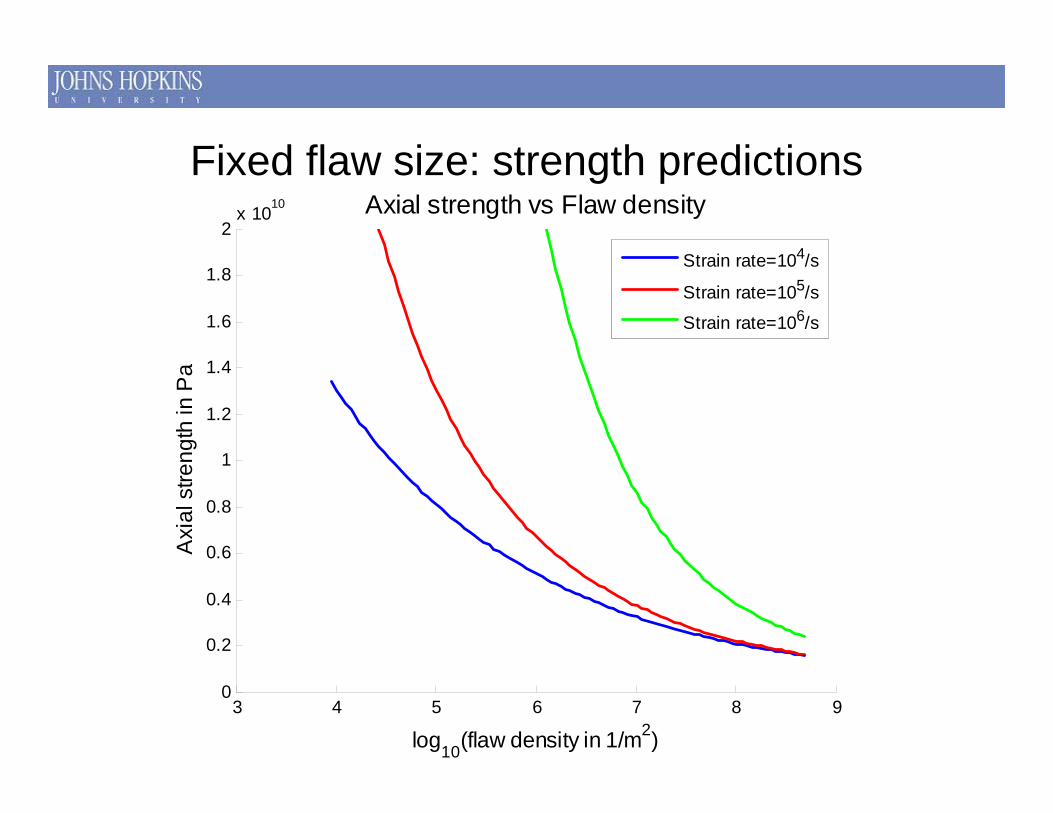
Fixed flaw size: strength predictions
3 4 5 6 7 8 90
0.2
0.4
0.6
0.8
1
1.2
1.4
1.6
1.8
2x 10¹⁰ Axial strength vs Flaw density
log10(flaw density in 1/m2)
Axi
al s
treng
th in
Pa
Strain rate=104/s
Strain rate=105/s
Strain rate=106/s

C.O.V. of Strength vs Element Size/s

/s
C.O.V. of Strength vs Element Size

Mesh dependency in models of failure
The assumption of homogeneous material properties in modeling localized failure leads to mesh dependencies
•Brannon’s work shows improved mesh independency when strength is allowed to vary spatially
In FEM, each element has a different strength – varies randomly!

••Random variations in material properties can lead to variabilityRandom variations in material properties can lead to variability in in structural behavior (e.g., local stress in structural behavior (e.g., local stress in elastoplasticelastoplastic composite)composite)
••Ignoring random variations in local strength can lead to numericIgnoring random variations in local strength can lead to numerical al problems (e.g., mesh dependency in shear bands, dynamic failure problems (e.g., mesh dependency in shear bands, dynamic failure of brittle materials)of brittle materials)
••Tools have been developed for quantifying the random variations Tools have been developed for quantifying the random variations in these properties, using movingin these properties, using moving--window approachwindow approach
••Stochastic simulation an effective tool for quantifying probabilStochastic simulation an effective tool for quantifying probability of ity of failurefailure
••Windowing of Windowing of elastoplasticelastoplastic composites still under studycomposites still under study
••Finite element analyses based on random strength of brittle Finite element analyses based on random strength of brittle materials yet to be developedmaterials yet to be developed
CONCLUSIONSCONCLUSIONS