stochastic signals and systems - tu dresden · a random variable x is given with the cumulative ......
TRANSCRIPT

Communications Theory
Faculty of Electrical and Computer Engineering Communications Laboratory
Chair of Communications Theory
STOCHASTIC SIGNALS AND SYSTEMSDipl.-Ing. Mathias Kortke
Prof. Dr.-Ing. habil. Rüdiger Hoffmann
Prof. Dr.-Ing. Eduard Jorswieck
October 2017


CONTENTS
8 Stochastic Signals 4
9 Static Systems 10
10 Dynamic Systems 13
E Examinations 18
F Formulary 24
G Formulary of LTI-Systems 32
BIBLIOGRAPHY
[1] WUNSCH, G. ; SCHREIBER, H.: Digitale Systeme. 5. Auflage. Dresden : TUD-press Verlag der Wissenschaften GmbH, 2006 (TUDpress Lehrbuch). – ISBN 10:3938863846, ISBN 13: 978–3938863848
[2] WUNSCH, G. ; SCHREIBER, H.: Analoge Systeme. 4. Auflage. Dresden : TUD-press Verlag der Wissenschaften GmbH, 2006 (TUDpress Lehrbuch). – ISBN 10:3938863676, ISBN 13: 978–3938863671
[3] WUNSCH, G. ; SCHREIBER, H.: Stochastische Systeme. 4. Auflage. Berlin :Springer-Verlag, 2005 (Springer-Lehrbuch). – ISBN 10: 354029225X, ISBN 13: 978–3540292258
[4] WUNSCH, G. ; SCHREIBER, H.: Stochastische Systeme. 3. Auflage. Berlin Heidel-berg : Springer-Verlag, 1992 (Springer-Lehrbuch)
[5] GALLAGER, R. G.: Stochastic Processes, Theory for Applications. Cambridge, UK :Cambridge University Press, 2013. – ISBN 978–1–107–03975–9
ABBREVIATIONSACF Autocorrelation functionCCF Cross-correlation functionCDF Cumulative distribution functionPDF Probability density function
1


EXERCISES

8 STOCHASTIC SIGNALS
8.1. The illumination of a room is supplied by two serially connected lamps L1 and L2,independently failing with the probabilities p1 and p2. What is the probability for thefailure of the room’s illumination?
8.2. An electric circuit (see Figure 8.2) contains fourohmic resistors, independently failing with the prob-abilities p1, p2, p3, and p4 (i. e. Ri → ∞, i ∈1, 2, 3, 4). Calculate the probability for the discon-tinuity of the current I!
R3
R2R1
R4
I
Figure 8.2
8.3. Two shooters fire at a target. The probability to hit the target is 0.8 for the firstshooter and 0.9 for the second one. What is the probability that the target will be hit?
8.4. Numerically coded control commands of the type 111 and 000 are transmitted viaa disturbed channel. The transmission probability for the first type is 0.7 and for thesecond one is 0.3. Each token (0 or 1) is transferred correctly with a probability of0.8.
a) What is the probability for the reception of the control command 101?
b) If the received code is 101, what is the probability that
α) 111, β) 000
was transmitted?
8.5. A random variable X is given with the cumulative distribution function (CDF) FX :
FX (ξ) =
0 ξ ≤ −1,1− ξ2 −1 < ξ ≤ 0,1 ξ > 0.
a) Calculate the probability density function (PDF) fX and draw a sketch!
b) What is the probability for X having a value smaller than −12?
c) Calculate the probability P−1
3 ≤ X < 2
using
α) the cumulative distribution function (CDF),β) the probability density function (PDF)!
8.6. Calculate the expected value (mean) E(X ), the quadratic mean E(X 2), and thevariance Var(X )
4 8 Stochastic Signals

a) of a discrete random variable X with corresponding CDF FX according to Fig-ure 8.6a,
b) of a continuous random variable X with corresponding CDF FX
FX (ξ) =
0 ξ ≤ 0,ξ2 0 < ξ ≤ 1,1 ξ > 1
according to Figure 8.6b!
1
-1 0 1 2 3 4ξ ξ
0.40.3
1
FX (ξ) FX (ξ)
10
0.9
Figure 8.6a Figure 8.6b
8.7. The life cycle (the time from start-up to the failure) of an electronic system is givenby the random variable X with the PDF fX :
fX (x) =
a e−ax x ≥ 0 (a > 0)
0 x < 0.
The average lifetime is 10 years. Calculate the probability that
a) the system operates reliably for at least 3 years,
b) the system will operate reliably for another 2 years, if it is known that the systemhas been working for 3 years already!
8.8. The life cycle of a component can be approximated by the random variable X withthe PDF fX :
fX (x) =
λ2x e−λx x > 00 x ≤ 0
(λ = 0.25/ year).
5

a) Calculate the probability that the component does not fail within 6 years!
b) A device consists of 4 of these components, failing independently of each other.Calculate the probability that the device does not fail within 6 years!
8.9. A collection of electronic devices contains rejects of 5% (faulty devices). At leasthow many devices should a random sample contain (i. e. how many devices have tobe checked) in order to find at least one faulty device with a probability of not less than0.9?
8.10. A random vector X = (X1, X2) is uniformly distributed in a rectangle B1 (Fig-ure 8.10), i. e., the PDF is
fX (x1, x2) =
1ab (x1, x2) ∈ B1
0 (x1, x2) /∈ B1(a > b > 0).
B2
B1
x1
b
0 b a
x2
Figure 8.10
a) What is the probability for X to lie within the quarter circle area B2?
b) Calculate the probability for X1 having a value greater than b (X2 arbitrary)!
8.11. Given a random vector X = (X1, X2) with the CDF FX .
Calculate as a function of FX
a) PX ∈ B1,
b) PX ∈ B1 |X ∈ B2!
(See Figure 8.11.)
b2
0 a1 a2
x1
B2
B1
b1
x2
Figure 8.11
8.12. During a message transmission, 1% of all characters are faultily received. Whatis the probability that in a text of 200 characters there isa) nob) at most one
faulty character.
8.13. A random vector X = (X1, X2) is uniformly distributed in a rectangle B, i. e. thePDF fX (x1, x2) is constant for (x1, x2) ∈ B. (See Figure 8.13.)
6 8 Stochastic Signals

a) What is the PDF fX ?
b) Calculate the marginal PDFs fX1 and fX2 anddraw a sketch for each!
c) Calculate PX1 ≥ 1!
d) Calculate the probability for X2 having avalue greater than X1!
B
x1320 1
1
x2
Figure 8.13
8.14. A random vector X = (X1, X2) is distributed in a rectangle B with the PDF fX :
fX (x1, x2) =
x1π
(x1, x2) ∈ B,0 (x1, x2) /∈ B.
a) Calculate fX1(x1 | x2) and fX2(x2 | x1). Find out whether thecomponents X1 and X2 of X are stochastically independentof each other!
b) Calculate the probability for X1 having a value smaller than0.5?
π
B
1
x2
0
−π
x1
Figure 8.14
8.15. A random vector X = (X1, X2, X3) is uniformly distributed inside the sphere x12 +
x22 + x3
2 ≤ R2, i. e., the PDF of X is constant inside the sphere. What is this PDF?
8.16. Given are three stochastically independent random variables X1, X2, and X3 withE(Xi) = 0 and Var(Xi) = σi
2 (i ∈ 1, 2, 3).
a) Calculate the variance Var(Y ) of Y = a1X1 + a2X2 + a3X3 (ai ∈ R)!
b) Determine specifically the variances Var(X1 + X2) and Var(X1 − X2)!
8.17. Consider a random process X = (Xt)t∈T with Xt = X (t) = X1 sin(ω0t − X2),wherein X1 and X2 are random variables uniformly distributed in the interval (0, 2π].Specify some realisations of X and draw their curves!
8.18. A noise voltage across an ohmic resistor R can be approximated by a stationaryrandom process X with the PDF fX :
fX (x, t) =12a
exp(−|x|
a
)(a > 0)
Calculate (for a fixed time t)
a) the probability, that the voltage exceeds a given value a0 > 0;
7

b) the expected value of the voltage;
c) the expected value of the power at R!
d) What is the result using a = 1 V, a0 = 2 V, and R = 3 ˙?
Note to b):∫
x e cx dx =e cx
c2(cx − 1) + C
Note to c):∫
x2 e cx dx =e cx
c3(x2c2 − 2cx + 2) + C
8.19. The circuit given in Figure 8.19 contains a noise voltage source and a noisecurrent source. The current flowing through R2
can be represented by the random process
I2 =U − IR1
R1 + R2
U and I are stationary (and jointly stationary)random processes with the correlation func-tions sU, sI, and sUI.
I
R1
R2
I2
U
Figure 8.19
a) Calculate sI2(τ) as a function of sU(τ), sI(τ), and sUI(τ)!
b) What is the mean value of the power at the resistor R2?
8.20. Given the random process Y :
Y (t) = X1 cosω0t + X2 sinω0t (ω0 ∈ R, constant),
wherein X1 and X2 are independent random variables with
E(X1) = E(X2) = 0 and E(X12) = E(X2
2) = σ2.
a) Calculate the expected value E(Y (t)) = mY (t)!
b) Calculate the autocorrelation function E(Y (t1)Y (t2)) = sY (t1, t2)!
c) Is the process Y wide-sense stationary?
8.21. Let sX be the autocorrelation function of a stationary random process X =(Xt)t∈T . Show that
| sX (τ) | ≤ sX (0) (τ = t2 − t1; t1, t2 ∈ T ) holds.
Note:Calculate the (nonnegative) expression E
((X (t)± X (t + τ))2
)≥ 0!
8 8 Stochastic Signals

8.22. A noise voltage across an ohmic resistor R can be approximated by a stationaryrandom process U with a zero mean and the power density spectrum SU:
SU(ω) =
S0 −ω0 ≤ ω ≤ +ω0
0 ω < −ω0, ω > +ω0(S0 > 0, constant).
a) What is the power density spectrum and the autocorrelation function of the currentI through the ohmic resistor R!
b) Calculate the mean power input of R!
8.23. The current through an ohmic resistor R can be approximated by a stationaryGaussian process X , where
mX (t) = 0 and sX (τ) = A2 e−α|τ | (A,α ∈ R, α > 0).
a) Calculate the power density spectrum SX (ω)!
b) Calculate the mean power input of R!
c) What is the PDF fX (x, t)?
d) What is the PDF fX (x1, t1; x2, t2)? (τ = t2 − t1)
8.24. Let X be a stationary Gaussian process with a zero mean and the autocorrelationfunction sX :
sX (τ) = A2 e−α|τ |(
cos βτ − α
βsin β|τ |
)(A > 0, α > 0, β > 0).
Calculate the probability for X (t) having a value greater than b!Numerical example: A = 1 V, α = 104 s−1, β = 105 s−1, b = 0.5 V.Note: Gauss error function
Φ(u) =1√2π
u∫0
exp(−v2
2
)dv ;
Φ(u) = −Φ(−u); Φ(∞) = 0.5; Φ(0.5) ≈ 0.1915
9

9 STATIC SYSTEMS
9.1. A non-linear static system (see Figure 9.1a) is given with an exponential charac-teristic curve ϕ : R→ R, y = ϕ(x) = e 3x .
X ϕ Y
210
1
x
fX (x)
Figure 9.1a Figure 9.1b
The input values of this system can be approximated by a random variable X with atriangular distribution (the corresponding PDF is shown in Figure 9.1b). Calculate thePDF of the random variable Y at the output of the system! Draw the curve of the PDFfY (y)!
9.2. A static system is shown in Figure 9.2. The input values of this system are givenby the random vector X = (X1, X2) with the PDF fX .Calculate the PDF fY of the random vector Y =(Y1, Y2) at the output of the system
a) generally for any desired fX ,
b) specifically for
fX (x1, x2) =1
2πσ2exp
(−x1
2 + x22
2σ2
)(σ > 0)!
+X2
X1
a Y2
Y1
Figure 9.2
9.3. The RANDOM function of a computer generates pseudo-random numbers whichcan approximately be characterised as a uniformly distributed random variable in theinterval (0, 1).Which arithmetic operation has to be applied to these numbers in order to obtainrandom numbers with a Cauchy distribution with the PDF fY :
fY (y) =1π
1y2 + 1
? (see Figure 9.3)
X y = ϕ(x) =? Y1
10
fX (x)
x0
y
fY (y)
Figure 9.3
9.4. A static system is shown in Figure 9.4. X1 and X2 are stochastically independentrandom variables for which E(X1) = E(X2) = 0 and Var(X1) = Var(X2) = σ2 hold.
10 9 Static Systems

a) Calculate E(Y1) and E(Y2)!
b) Calculate Var(Y1) and Var(Y2)!
c) Calculate Cov(Y1, Y2)!
d) What is the correlation coefficient%(Y1, Y2)?
e) Calculate fY (y1, y2), if
fX (x1, x2) =1
2πσ2exp
(−x1
2 + x22
2σ2
)!
+
+
β
α Y1
Y2
X1
X2 −β
Figure 9.4
9.5. The input of a rectifier shown in Figure 9.5 with the characteristic curve ϕ:
y = ϕ(x) =
e ax − 1 x ≥ 0,0 x < 0
can be approximated by a non-stationaryrandom process X with the PDF fX , withfX (x, t) = 0 for all t ∈ T if x < 0.
ϕ
0
YX
yϕ
x
Figure 9.5
a) Calculate fY (y, t) in general!
b) What is the result specifically for
fX (x, t) =
α
1 + β2t2exp
(−αx
1 + β2t2
)x ≥ 0,
0 x < 0?
For the constants a > 0, α > 0, β > 0 hold.
9.6. The autocorrelation function sX and the PDF fX of the stationary random processX shown in Figure 9.6 are given as:
sX (τ) = 2A2 e−α|τ | cos βτ
fX (x, t) =1
2Aexp
(−|x|
A
)(A > 0, α > 0, β > 0).
(X ⇔ U1, Y ⇔ U2)
YR1
R2X
Figure 9.6
a) Calculate the autocorrelation function of the process Y !
b) Calculate the one-dimensional PDF of the process Y !
11

c) For an arbitrary time t and (a > 0), calculate the probability for Y (t) > a.
d) What is the result of c), if A = 1 V, a = 2 V, R1 = 1 ˙, and R2 = 2 ˙ are given?
9.7. The circuit shown in Figure 9.7 contains two adders and two ideal amplifiers withthe amplification factors v1 and v2. The processes X (input process), U, and V (distur-bance processes) are stationary and independent random processes with the meanvalues mX = mU = mV = 0.
++
U V
v1 v2 YX
Figure 9.7
The power density spectrum of the process X is given by
SX (ω) =A2
ω2 + a2(A > 0, a > 0)
whereas U and V are white noise processes with
SU(ω) = SV (ω) = S0 (S0 > 0).
a) Calculate the cross-correlation function of the processes X and Y !
b) Calculate the power density spectrum of the process Y !
9.8. A noise voltage across a diode with the current voltage characteristic
i = ϕ(u) = I0
(exp
(uU0
)− 1)
(I0 > 0, U0 > 0)
can be approximated by a stationary random process U with the PDF fU:
fU(u, t) =
1
U00 ≤ u ≤ U0
0 u < 0, u > U0
.
a) Calculate the PDF fI of the current I and draw the curve of fI(i, t)!
b) Calculate the mean of the current I by using the equation
E(ϕ(X )) =
∞∫−∞
ϕ(x)fX (x) dx!
12 9 Static Systems

10 DYNAMIC SYSTEMS
10.1. Show that a stationary random process X with the autocorrelation function sX ismean-square continuous, if and only if sX (τ) is continuous in τ = 0.Note: Examine the equation
||X (t + τ)− X (t)||2 = E((X (t + τ)− X (t))2
)for τ → 0!
10.2. Let X be a mean-square differentiable random process with mean mX and auto-correlation function sX . Show that,
a) mX (t) =ddt
mX (t),
b) sXX (t1, t2) =∂
∂t1sX (t1, t2) and
c) sXX (t1, t2) =∂
∂t2sX (t1, t2) are true!
d) How will these equations be changed, if X is stationary!
10.3. A noise voltage across an ideal capacitor C canbe approximated by a stationary Gaussian process Uwith mU(t) = 0 and
sU(τ) = A2 exp(−aτ 2
)(A ∈ R, a > 0)
(see Figure 10.3).
τ0
sU(τ)
Figure 10.3
For the current I through C, calculate
a) the mean mI (mI(t) =?),
b) the cross-correlation functions sIU and sUI (sIU(τ) =?, sUI(τ) =?) (Draw curves!),
c) the autocorrelation function sI (sI(τ) =?) (Draw a curve!), and
d) the PDF fI (fI(i, t) =?)!
10.4. The circuit (zero state at t = 0) given in Fig-ure 10.4 contains a noise voltage source whichcan be represented by the stationary random pro-cess U with the autocorrelation function sU:
sU(τ) = 2U02 e−a|τ | (a > 0).
U C R
L
Figure 10.4
Calculate the power density spectra of the voltage U and the current I through R!
13

Note: Correspondence of the Fourier transform:
e−a|τ |
2aω2 + a2
10.5. A noise voltage across the terminals of a RLC two terminal network (see Figure10.5) can be represented by the stationaryrandom process U with a constant powerdensity spectrum SU(ω) = S0.
a) Calculate the power density spectrumof the total current I!
b) Calculate the autocorrelation functionof the current IR!
Note: See exercise 10.4.
L
IR
I R
C
U
Figure 10.5
10.6. The input of a linear dynamic system with the impulse response g (see Fig-ure 10.6) can be approximated by a stationary random process X with the autocorrela-tion function sX .Calculate the cross-correlation function sXY in integral form as a function of sX and g!Determine the result specifically for sX (τ) = S0 δ(τ)!Note:
Y (t) =
∞∫0
g(λ)X (t − λ) dλ
for any stationary random process at arbitrary time t.
g YX
Figure 10.6
10.7. The input voltage X (⇔ U1) of a RC network shown in Figure 10.7 can be approx-imated by a stationary Gaussian process with the power density spectrum SX (ω) = K(white noise) and the mean mX (t) = 0.
a) Calculate the power density spectrumSY (ω) of the output voltage Y (⇔ U2)!
b) Calculate the autocorrelation function sY
of the process Y !
c) Specify fY (y, t) and fY (y1, t1; y2, t2)!
C R U2
(X ⇔ U1, Y ⇔ U2)
U1
R
Figure 10.7
Note: Correspondence of the Fourier transform:
1ω2 + a2
12a
e−a|τ | (a > 0)
14 10 Dynamic Systems

10.8. In the circuit (zero state at t = 0) shown in Figure 10.8, the variable X denotesa stationary random process with a constant power density spectrum SX (ω) = S0.Calculate the power density spectrum of the process Y at the output of this system!∫ ∫
YX 4 + +
−323
Figure 10.8
10.9. Given an electric network with the thermally noisy ohmic resistors R1, R2, andR3 shown in Figure 10.9, calculate the power density spectrum of the noise voltage Uacross the terminals AB and draw a noise equivalent circuit!
L R3
R2 R1
A B
Figure 10.9
10.10. For the quantitative description of a mean-square ergodic random process U,the effective noise voltage
Ueff =
√u2(t) =
√E (U2(t)).
is used.Calculate the effective noise voltage
a) in case of a given autocorrelation function sU:
sU(τ) = A2 e−α|τ | cos βτ (A > 0, α > 0, β > 0);
Numerical example: A = 1 V, α = 10−3 s−1, β = 10−4 s−1;
b) for an ohmic resistor R in a low frequency range, i. e. the power density spectrumSU is
SU(ω) =
2kTR |ω| < ω0,0 |ω| > ω0.
Numerical example: R = 1 M˙, f0 = ω02π = 20 kHz, T = 300 K, k = 1.38 ·10−23 Ws/ K
10.11. Figure 10.11 shows a block diagram of a circuit for measuring the root meansquare (RMS) of weak signals. In this diagram, X denotes the input signal, whoseRMS has to be determined, whereas U and V denote the noise signals of the two
15

amplifiers with the amplification factors v1 and v2. The given signals X , U, and Vcan be interpreted as independent stationary and ergodic random process with a zeromean. Show that the output signal is proportional to
Xeff =
√x2(t) =
√E (X 2(t))
and independent of the noise voltages of the amplifiers!
X
v1
v2
× E(. . . )
+
+
U
V
Y√
(. . . )
Figure 10.11
11.1.
A digital second order band pass fil-ter (see Figure 11.1) is given with thetransfer function G:
G(z) =z2 − 1
2.1 z2 + 1.9
BandpassyS(k)xS(k)
XN(k) YN(k)
Figure 11.1
The input x of the digital filter is the sum of a discrete time signal xS:
xS(k) = X sin Ωk (X = 1, Ω =12π)
and a discrete time random signal (caused by a previous analog to digital conversion),which can be approximated by a stationary discrete time random process XN withuncorrelated signal values (“white noise”). It is assumed, that XN(k) is uniformly dis-tributed in the intervall
(−1
2∆, +12∆]
(numerical example: ∆ = 2−10).
a) Calculate the amplitude frequency response of the digital filter and draw a sketch!
b) Calculate the signal-to-noise ratio (SNR) at the input and at the output of the filter!Note:
a = 20 lgXS,eff
XN,eff= 10 lg
xS2(k)
xN2(k)
16 10 Dynamic Systems

EXAMINATIONS

E EXAMINATIONS
Stochastic Signals and Systems
1st final examination
1. By playing dice with two independent dice, a discrete two-dimensional randomvariable (X1, X2) is defined.
a) Calculate the expected values E(X1) and E(X2)!
b) Calculate the variances Var(X1) and Var(X2)!
c) Is it possible to determine the correlation coefficient %(X1, X2) without any calcula-tion? (Specify the reasons!)
2. A non-linear static system with one input and one output is given (see Figure 2).The input of the system is the random variable X , which is uniformly distributed in theinterval [0, 3]. Which characteristic curve ϕ is required for the system to produce arandom variable Y with the probability density function (PDF)
fY (y) =
0.5y 0 ≤ y ≤ 2
0 y < 0, y > 2
at the output?
X Yj
Figure 2: Static system
a) Draw the curves of fX (x), FX (x), fY (y), and FY (y)!
b) Calculate y = ϕ(x) and also draw the curve of this system function! In case ofmultiple results, choose a suitable solution!
3. A noise voltage across an ohmic resistor R can be approximated by a stationaryrandom process U with a zero mean and the power density spectrum SU:
SU(ω) =
S0 if −ω0 ≤ ω ≤ ω0
0 if ω < −ω0, ω > ω0(S0 > 0, constant)
a) What is the power density spectrum and the autocorrelation function of the currentI through the ohmic resistor R!
b) Calculate the mean power input of R!
18 E Examinations

4. The circuit shown in Figure 4 contains two adders and two ideal amplifiers with theamplification factors v1 and v2.The processes X (input process), U, and V (disturbance processes) are stationary andindependent random processes with the mean values mX = mU = mV = 0.The power density spectrum of the process X is given by
SX (ω) =A2
ω2 + a2(A > 0, a > 0)
whereas U and V are white noise processes with
SU(ω) = SV (ω) = S0 (S0 > 0).
X
U
+ v1 +
V
Yv2
Figure 4: Static system
a) Calculate the cross-correlation function of the processes X and Y !
b) Calculate the power density spectrum of the process Y !
5. In the circuit (zero state at t = 0) shown in Figure 5, the variable X denotes a station-ary random process with a constant power density spectrum SX (ω) = S0. Calculatethe power density spectrum of the process Y at the output of this system!
X + Y4
0,3
Figure 5: Circuit
6. Figure 6a shows a RLC two terminal network with two thermally noisy ohmic resis-tors at the same absolute temperature T . Calculate the power density spectra of thenoise sources in the noise equivalent circuits given in the Figures 6b and 6c!
R
R
C1
2
R
R
C1
2
SU
R
R
C1
2
SI
a) b) c)
Figure 6: a) RLC two terminal network b) and c) Noise equivalent circuits
19

Stochastic Signals and Systems
2nd final examination
1. The probability density function (PDF) fX of the random variable X is given as:
fX (x) =
0.50 0 < x ≤ 10.25 1 < x ≤ 3
0 x ≤ 0, x > 3.
a) Draw a sketch of the PDF of this random variable!
b) Calculate the corresponding cumulative distribution function (CDF) and draw asketch!
c) Calculate the probability PX ≥ 2!
d) Calculate the expected value E(X )!
2. The random variables X1, X2, and X3 are stochastically independent of each otherwith the expected values
E(X1) = E(X2) = E(X3) = 0
and the variances
Var(X1) = Var(X2) = Var(X3) = σ2.
a) Calculate E(Y ) and Var(Y ) at the output of the static system shown in Figure 2!
b) Calculate the correlation coefficient % = %(X1, Y ) of the random variables X1 and Y !
c) How do the results of a) and b) change, if the amplifier V2 in Figure 2 fails (i. e.V2 = 0)?
X
X
X
Y2 2 2
1 1 1
3 33
++V
V
V V = 3
V = -2
V = 3
Figure 2 Static system
3. The noise voltage U across the RL series connection shown in Figure 3 has a con-stant power density spectrum SU(ω) = S0 = const.
a) Calculate the power density spectra of the partial voltages UL, UR and of the currentI!
b) Calculate the autocorrelation function of the current I!
20 E Examinations

c) Calculate the mean power input of R!
U
L
R I
Figure 3 RL series connection
4. Calculate the probability density function (PDF) fY (y, t) of the random process
Y = aX + b (a ∈ R, b ∈ R),
if X is a stationary Gaussian process with a zero mean (i. e. mX (t) = 0) and theautocorrelation function sX :
sX (τ) = A2 exp(−α|τ |) (A > 0, α > 0)?
5.
a) What is a stationary random processes?
b) Which properties do the expected value and the autocorrelation function of a sta-tionary random process have?
c) Calculate the autocorrelation function of a stationary random process X , if itspower density spectrum is given by
SX (ω) =
S0 = const −ω0 ≤ ω ≤ ω0
0 ω > ω0, ω < −ω0!
Draw qualitatively a sketch of the autocorrelation function!
6. Two thermally noisy ohmic resistors R1 with the absolute temperature T1 and R2
with the absolute temperature T2 are connected in parallel (Figure 6). Calculate thepower density spectrum SU(ω) of the noise voltages U across the parallel connection!
R
R
T
T
1 1,
,2 2
Figure 6 Thermally noisy ohmic resistors
21


FORMULARY

F FORMULARY
Formulary of Stochastic Signals and Systems (1)
Preliminaries of the Probability Calculus
P(A) = 1− P(A)
P(A ∪ B) = P(A) + P(B)− P(A ∩ B)
= P(A) + P(B), if A ∩ B = ∅ (A, B mutually exclusive)
P(A \ B) = P(A)− P(A ∩ B)
= P(A)− P(B), if B ⊂ A
P(A ∩ B) = P(A|B)P(B) = P(B|A)P(A)
= P(A)P(B), if A and B are stochastically independent
P(A|B) =P(A ∩ B)
P(B)(P(B) 6= 0) conditional probability
P(B) =n∑
i=1
P(B|Ai)P(Ai) formula of total probability
P(Ai |B) =P(B|Ai)P(Ai)
P(B)Bayesian formula
One-dimensional Random Variables
FX (ξ) = PX < ξ =
ξ∫−∞
fX (x) dx
Pa ≤ X < b =
b∫a
fX (x) dx = FX (b)− FX (a)
Specific Distributions
fX (x) =1√
2π σexp
(−(x −m)2
2σ2
)(σ > 0) normal distribution (Gaussian d.)
PX = k =
(nk
)pk(1− p)n−k (k = 0, 1, 2, . . . , n) binomial d. (Bernoulli d.)
PX = k =λk
k!e−λ (k = 0, 1, 2, . . .) Poisson distribution
24 F Formulary

Moments of One-dimensional Random Variables
X discrete X continuousGeneral Moments:
Expected value m = E(X )∑
i
xiPX = xi∞∫
−∞
xfX (x) dx
Moment of n-th Order mn = E(X n)∑
i
xni PX = xi
∞∫−∞
xnfX (x) dx
Central Moments:
Dispersion, Variance
µ2 = E((X −m)2) = Var(X )∑
i
(xi −m)2PX = xi∞∫
−∞
(x −m)2fX (x) dx
Central moment of n-th order
µn = E((X −m)n)∑
i
(xi −m)nPX = xi∞∫
−∞
(x −m)nfX (x) dx
Characteristic function:
ϕX (λ) = E(e jλX
) ∑i
e jλxi PX = xi∞∫
−∞
e jλxfX (x) dx
Two-dimensional Random Variables X = (X1, X2)
FX (ξ1, ξ2) = PX1 < ξ1, X2 < ξ2 =
ξ1∫−∞
ξ2∫−∞
fX (x1, x2) dx2 dx1
Pa1 ≤ X1 < b1, a2 ≤ X2 < b2 =
b1∫a1
b2∫a2
fX (x1, x2) dx2 dx1
= FX (b1, b2)− FX (b1, a2)− FX (a1, b2) + FX (a1, a2)
Marginal probability density function
fX1(x1) =
∞∫−∞
fX (x1, x2) dx2 fX2(x2) =
∞∫−∞
fX (x1, x2) dx1
Conditional probability density function
fX1(x1|x2) =fX (x1, x2)
fX2(x2)fX2(x2|x1) =
fX (x1, x2)
fX1(x1)
Correlation coefficient
%(X1, X2) =Cov(X1, X2)√
Var(X1) Var(X2)=
E((X1 −mX1)(X2 −mX2))√E ((X1 −mX1)
2) E ((X2 −mX2)2)
25
Formulary of Stochastic Signals and Systems (2)
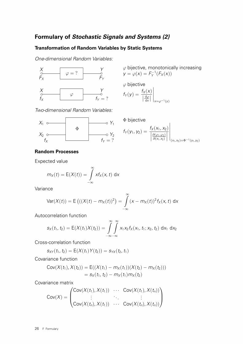
Transformation of Random Variables by Static Systems
One-dimensional Random Variables:
ϕ = ?
ϕY
fY = ?
Y
FY
X
FX
X
fX
ϕ bijective, monotonically increasingy = ϕ(x) = F−1
Y (FX (x))
ϕ bijective
fY (y) =fX (x)∣∣ dϕ
dx
∣∣∣∣∣∣∣x=ϕ−1(y)
Two-dimensional Random Variables:
X1
X2
ΦY2
Y1
fY = ?fX
Φ bijective
fY (y1, y2) =fX (x1, x2)∣∣∣∂(ϕ1,ϕ2)∂(x1,x2)
∣∣∣∣∣∣∣∣∣(x1,x2)=Φ−1(y1,y2)
Random Processes
Expected value
mX (t) = E(X (t)) =
∞∫−∞
xfX (x, t) dx
Variance
Var(X (t)) = E(((X (t)−mX (t))2
)=
∞∫−∞
(x −mX (t))2fX (x, t) dx
Autocorrelation function
sX (t1, t2) = E(X (t1)X (t2)) =
∞∫−∞
∞∫−∞
x1x2fX (x1, t1; x2, t2) dx1 dx2
Cross-correlation function
sXY (t1, t2) = E(X (t1)Y (t2)) = sYX (t2, t1)
Covariance function
Cov(X (t1), X (t2)) = E((X (t1)−mX (t1))(X (t2)−mX (t2)))
= sX (t1, t2)−mX (t1)mX (t2)
Covariance matrix
Cov(X ) =
Cov(X (t1), X (t1)) · · · Cov(X (t1), X (tn))... . . . ...
Cov(X (tn), X (t1)) · · · Cov(X (tn), X (tn))
26 F Formulary

Stationary Random Processes
Expected value E(X (t)) = mX (t) = mX (= const.)
Variance Var(X (t)) = σX2 (= const.)
Autocorrelation function sX (τ) = E(X (t)X (t + τ))
Cross-correlation function sXY (τ) = E(X (t)Y (t + τ)) = sYX (−τ)
Power density spectrum SX (ω) =
∞∫−∞
sX (τ) e− jωτ dτ
(Theorem of Wiener/Chintschin) sX (τ) =1
2π
∞∫−∞
SX (ω) e jωτ dω
Gaussian Processes
fX (x1, t1; . . . ; xn, tn) =1√
(2π)n det Cexp
(−1
2(x −m)C−1(x −m)′
)With: (x −m) = (x1 −mX (t1) · · · xn −mX (tn)) row matrix
(x −m)′ transposed matrix of (x −m)
C = Cov(X ) covariance matrix with the elementsCov(X (ti), X (tj)) = sX (ti , tj)−mX (ti)mX (tj)
Markov Processes
fX (xn, tn|x1, t1; . . . ; xn−1, tn−1) = fX (xn, tn|xn−1, tn−1) (t1 < t2 < · · · < tn)
fX (x1, t1; . . . ; xn, tn) =
fX (xn, tn|xn−1, tn−1) · fX (xn−1, tn−1|xn−2, tn−2) · · · fX (x2, t2|x1, t1) · fX (x1, t1)
fX (x1, t1; . . . ; xn, tn) =fX (xn, tn; xn−1, tn−1)
fX (xn−1, tn−1)· · · fX (x2, t2; x1, t1)
fX (x1, t1)· fX (x1, t1)
27
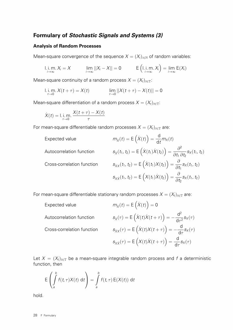
Formulary of Stochastic Signals and Systems (3)
Analysis of Random Processes
Mean-square convergence of the sequence X = (Xi)i∈N of random variables:
l. i.m.i→∞
Xi = X limi→∞||Xi − X || = 0 E
(l. i.m.
i→∞Xi
)= lim
i→∞E(Xi)
Mean-square continuity of a random process X = (Xt)t∈T:
l. i.m.τ→0
X (t + τ) = X (t) limτ→0||X (t + τ)− X (t)|| = 0
Mean-square differentiation of a random process X = (Xt)t∈T:
X (t) = l. i.m.τ→0
X (t + τ)− X (t)τ
For mean-square differentiable random processes X = (Xt)t∈T are:
Expected value mX (t) = E(
X (t))
=d
dtmX (t)
Autocorrelation function sX (t1, t2) = E(
X (t1)X (t2))
=∂2
∂t1 ∂t2sX (t1, t2)
Cross-correlation function sXX (t1, t2) = E(
X (t1)X (t2))
=∂
∂t1sX (t1, t2)
sXX (t1, t2) = E(
X (t1)X (t2))
=∂
∂t2sX (t1, t2)
For mean-square differentiable stationary random processes X = (Xt)t∈T are:
Expected value mX (t) = E(
X (t))
= 0
Autocorrelation function sX (τ) = E(
X (t)X (t + τ))
= − d2
dτ 2sX (τ)
Cross-correlation function sXX (τ) = E(
X (t)X (t + τ))
= − ddτ
sX (τ)
sXX (τ) = E(
X (t)X (t + τ))
=d
dτsX (τ)
Let X = (Xt)t∈T be a mean-square integrable random process and f a deterministicfunction, then
E
b∫a
f (t, τ)X (t) dt
=
b∫a
f (t, τ) E(X (t)) dt
hold.
28 F Formulary
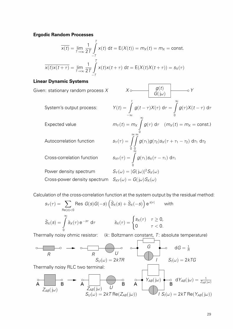
Ergodic Random Processes
x(t) = limT→∞
12T
T∫−T
x(t) dt = E(X (t)) = mX (t) = mX = const.
x(t)x(t + τ) = limT→∞
12T
T∫−T
x(t)x(t + τ) dt = E(X (t)X (t + τ)) = sX (τ)
Linear Dynamic Systems
Given: stationary random process X X YG( jω)g(t)
System’s output process: Y (t) =
t∫−∞
g(t − τ)X (τ) dτ =
∞∫0
g(τ)X (t − τ) dτ
Expected value mY (t) = mX
∞∫0
g(τ) dτ (mX (t) = mX = const.)
Autocorrelation function sY (τ) =
∞∫0
∞∫0
g(τ1)g(τ2)sX (τ + τ1 − τ2) dτ1 dτ2
Cross-correlation function sXY (τ) =
∞∫0
g(τ1)sX (τ − τ1) dτ1
Power density spectrum SY (ω) = |G( jω)|2SX (ω)
Cross-power density spectrum SXY (ω) = G( jω)SX (ω)
Calculation of the cross-correlation function at the system output by the residual method:
sY (τ) =∑
Re(s)<0
Res G(s)G(−s)(
SX (s) + SX (−s))
e s|τ | with
SX (s) =
∞∫0
sX (τ) e−sτ dτ sX (τ) =
sX (τ) τ ≥ 0,0 τ < 0.
Thermally noisy ohmic resistor: (k: Boltzmann constant, T : absolute temperature)
R RI
UG dG = 1
R
SI(ω) = 2kTGSU(ω) = 2kTR
Thermally noisy RLC two terminal:
A B A BZAB( jω) ZAB( jω) U
SU(ω) = 2kT Re(ZAB( jω))
AYAB( jω)
BdYAB( jω) = 1
ZAB( jω)
I SI(ω) = 2kT Re(YAB( jω))
29


FORMULARY OF LTI-SYSTEMS

G FORMULARY OF LTI-SYSTEMS
Formulary of Analog Signals and Systems (1)
Fourier Transform:
X (ω) =
∞∫−∞
x(t) e− jωt dt
x(t) =1
2π
∞∫−∞
X (ω) e jωt dω
Rules of the Fourier Transform:
No. x(t) X (ω) Remark
1 αx1(t) + βx2(t) αX1(ω) + βX2(ω) Linearity
2 x(t − τ) e− jωτX (ω) Displacement law(time shift)
3 x(t) e jω0t X (ω − ω0) Displacement law(frequency shift)
4 x(at)1|a|
X(ω
a
)Similarity law (a 6= 0)
5 x(t) jωX (ω) Differentiation law
6
t∫−∞
x(τ) dτ1jω
X (ω) Integration law *)
7
∞∫−∞
x1(τ)x2(t − τ) dτ X1(ω)X2(ω) Convolution law(time domain)
8 x1(t)x2(t)1
2π
∞∫−∞
X1(u)X2(ω − u) du Convolution law(frequency domain)
9 If the correspondence x(t) X (ω) is true, thenthe correspondence X (t) 2πx(−ω) is true too.
Exchange law
*) It has to be proven that the Fourier transform of the integral on the left-hand side reallyexists!
32 G Formulary of LTI-Systems

Correspondences of the Fourier Transform:
No. x(t) X (ω)
1 δ(t) 1
2 1(t) πδ(ω) +1jω
3 Rect(
t2τ
)=
1 −τ ≤ t ≤ τ
0 t < −τ ∨ t > τ2τ
sin(ωτ)
ωτ= 2τ si(ωτ)
4ω0
πsi(ω0t) =
ω0
π· sin(ω0t)
ω0tRect
(ω
2ω0
)=
1 −ω0 ≤ ω ≤ ω0
0 ω < −ω0 ∨ ω > ω0(ω0 6= 0)
5
e−at t > 00 t < 0
1jω + a
(a > 0)
6 e−a|t| 2aω2 + a2
(a > 0)
71
t2 + a2
π
ae−a|ω| (a > 0)
8 e−at2
√π
ae−
ω2
4a (a > 0)
9 (1 + a|t|) e−a|t| 4a3
(ω2 + a2)2(a > 0)
10(
1 + a|t|+ 13
(at)2
)e−a|t| 16a5
3(ω2 + a2)3(a > 0)
11 e−a|t| cos(βt)2a(ω2 + a2 + β2)
(ω2 − a2 − β2)2 + 4a2ω2(a > 0)
12 e−a|t|(
cos(βt) +aβ
sin(β|t|))
4a(a2 + β2)
((ω − β)2 + a2)((ω + β)2 + a2)(a > 0)
13
a(
1− |t|τ
)−τ < t < τ
0 otherwise
4aω2τ
sin2(ωτ
2
)= aτ si2
(ωτ2
)(τ 6= 0)
14 cos(ω0t) π (δ(ω − ω0) + δ(ω + ω0))
15 sin(ω0t) jπ (δ(ω + ω0)− δ(ω − ω0))
33

Formulary of Analog Signals and Systems (2)
Laplace Transform:
X (s) =
∞∫0
x(t) e−st dt
x(t) =1
2π j
δ+ j∞∫δ− j∞
X (s) e st ds
Rules of the Laplace Transform:
No. x(t) X (s) Remark
1 αx1(t) + βx2(t) αX1(s) + βX2(s) Linearity
2 x(t − τ) (τ > 0) e−sτX (s) Displacement law
3 x(at)1a
X(s
a
)Similarity law (a > 0)
4 x(t) sX (s)− x(+0) Differentiation law
5
t∫0
x(τ) dτ1s
X (s) Integration law
6 e−atx(t) X (s + a) Attenuation law
7
t∫0
x1(τ)x2(t − τ) dτ X1(s)X2(s) Convolution law
8 x(t) =∑
i
Ress=si
[X (s) e st
]Residual formula,
where
Ress=si
[X (s) e st
]=
1(m− 1)!
lims→si
dm−1
dsm−1
[X (s) e st(s − si)
m]
with si : m-fold pole of X (s),
and X (s) rational with X (∞)→ 0.
34 G Formulary of LTI-Systems

Correspondences of the Laplace Transform:
No. x(t) X (s)
1 δ(t) 1
2 1(t)1s
3 t 1(t)1s2
4 e at 1(t)1
s − a
5 t e at 1(t)1
(s − a)2
6t n−1
(n− 1)!e at 1(t)
1(s − a)n
(n = 1, 2, 3, . . . )
7 cos at 1(t)s
s2 + a2
8 sin at 1(t)a
s2 + a2
9 cosh at 1(t)s
s2 − a2
10 sinh at 1(t)a
s2 − a2
11 e at cos βt 1(t)s − a
(s − a)2 + β2
12 e at sin βt 1(t)β
(s − a)2 + β2
13 e at
(cos βt +
aβ
sin βt)
1(t)s
(s − a)2 + β2
14 cos2 at 1(t)s2 + 2a2
s (s2 + 4a2)
15 sin2 at 1(t)2a2
s (s2 + 4a2)
16 cos(at + b) 1(t)s cos b − a sin b
s2 + a2
17 sin(at + b) 1(t)s sin b + a cos b
s2 + a2
181√πt
1(t)1√s
19 2
√tπ
1(t)1
s√
s
35

Formulary of Analog Signals and Systems (3)
Z-Transform:X (z) =
∞∑k=0
x(k)z−k
x(k) =1
2π j
∮c
X (z)zk−1 dz (k = 0, 1, 2, . . . )
Rules of the Z-Transform:
No. x(k) X (z) Remark
1 αx1(k) + βx2(k) αX1(z) + βX2(z) Linearity
2 x(k −m) z−mX (z) Displacement law (→)
3 x(k + m) zm
(X (z)−
m−1∑i=0
x(i)z−i
)Displacement law (←)
4 x(k + 1)− x(k) (z − 1)X (z)− zx(0) Forward difference
5 x(k)− x(k − 1)(1− z−1
)X (z) Backward difference
6k∑
i=0
x1(i)x2(k − i) X1(z)X2(z) Convolution law
7 akx(k) X(z
a
)Attenuation law
8k∑
i=0
x(i)z
z − 1X (z) Summation
9 kx(k) −zd
dzX (z) Differentiation law (frequency domain)
101k
x(k)
∞∫z
X (w)dww
Integration (frequency domain)
11 x(k) =∑
i
Resz=zi
[X (z)zk−1
]Residual formula,
where
Resz=zi
[X (z)zk−1
]=
1(m− 1)!
limz→zi
dm−1
dzm−1
[X (z)zk−1(z − zi)
m]
with zi : m-fold pole of X (z)zk−1.
36 G Formulary of LTI-Systems

Correspondences of the Z-Transform:
No. x(k) X (z)
1 δ(k) 1
2 1(k)z
z − 1
3 k 1(k)z
(z − 1)2
4 k2 1(k)z(z + 1)
(z − 1)3
5 ak 1(k)z
z − a
6 kak 1(k)az
(z − a)2
7 k2ak 1(k)az(z + a)
(z − a)3
8ak
k!1(k) e
az
9(
km
)ak 1(k)
amz(z − a)m+1
10 e ak 1(k)z
z − e a
11 k e ak 1(k)e az
(z − e a)2
12 ak sin Ωk 1(k)az sin Ω
z2 − 2az cos Ω + a2
13 ak cos Ωk 1(k)z(z − a cos Ω)
z2 − 2az cos Ω + a2
14 ak sinh βk 1(k)az sinh β
z2 − 2az cosh β + a2
15 ak cosh βk 1(k)z(z − a cosh β)
z2 − 2az cosh β + a2
16 (−1)k 1(k)z
z + 1
37

Formulary of Analog Signals and Systems (4)
Survey of Integral Transforms of Spectral Analysis
Continuous-time Discrete-timeSignal SignalFOURIER-Series DFT (FFT)
Perio
dic
resp
.Pe
riodi
-ca
llyC
ontin
ued
Sig
nal
X n =1T
∫T
x(t) e− jnω0t dt
x(t) =∞∑
n=−∞
X n e jnω0t
X (n) =1N
N−1∑k=0
x(k) e− j2π nkN
x(k) =N−1∑n=0
X (n) e j2π knN
FOURIER-Transform DTFT / z-Transform
Non
-per
iodi
cS
igna
l
X (ω) =
∞∫−∞
x(t) e− jωt dt
x(t) =1
2π
∞∫−∞
X (ω) e jωt dω
X (e jω) =∞∑
k=−∞
x(k) e− jωk∆t
=⇒∞∑
k=−∞
x(k) z−k = X (z)
x(k) =∆t2π
π∆t∫
− π∆t
X (e jω) e jωk∆t dω
=1
2πj
∮X (z) zk−1 dz
Sampling x(k) = x(t)|t=k ·∆t
Reconstruction (Sampling Series) x(t) =∞∑
k=−∞
x(k) si( π
∆t(t − k∆t)
)Energy E of the Energy Signal x continuous-time discrete-time
∞∫−∞
x2(t) dt∞∑−∞
∆t x2(k)
38 G Formulary of LTI-Systems

Presentation of Linear Continuous-time Systems
by means of a simple example
Block Diagram
x(t) +t∫−∞
( · ) dτ y(t)
p
State Equations
z(t) = p z(t) + x(t)y(t) = z(t)
Impulse Response
g(t) = L−1(G(s)) = e pt 1(t)
Differential Equation
y(t)− p · y(t) = x(t)Transfer Function
G(s) = Y (s)X (s)
= 1s−p
Presentation of Linear Discrete-time Systems
by means of a simple example
Block Diagram
x(k) + y(k)
S
State Equations
z(k + 1) = 1 z(k) + 1 x(k)y(k) = 1 z(k) + 1 x(k)
Impulse Response
g(k) = Z−1(G(z)) = 1(k)
Differential Equation
y(k)− y(k − 1) = x(k)
Transfer Function
G(z) = Y (z)X (z)
= zz−1
39

Formulary of Analog Signals and Systems (5)
Linear Time Invariant Systems with
Discrete Time Continuous Time
State equations:
z(k + 1) = Az(k) + Bx(k) z(t) = Az(t) + Bx(t)
y(k) = Cz(k) + Dx(k) y(t) = Cz(t) + Dx(t)
Fundamental matrix in the frequency domain:
Φ(z) = (zE − A)−1z Φ(s) = (sE − A)−1
Transfer matrix resp. transfer function:
G(z) = C(zE − A)−1B + D G(s) = C(sE − A)−1B + D
Solution of the 1st state equation in the frequency domain:
Z(z) = Φ(z)z(0) + Φ(z)z−1BX (z) Z(s) = Φ(s)z(0) + Φ(s)BX (s)
Input-output-equation in the frequency domain:
Y (z) = CΦ(z)z(0) + G(z)X (z) Y (s) = CΦ(s)z(0) + G(s)X (s)
Fundamental matrix (fundamental solution) in the time domain:
ϕ(k) = Ak ϕ(t) = e At = E + A t1!
+ A2 t2
2!+ . . .
Impulse response:
g(k) =
D k = 0Cϕ(k − 1)B k = 1, 2, . . .
g(t) = Cϕ(t)B + Dδ(t)
Solution of the 1st state equation in the time domain:
z(k) = ϕ(k)z(0) +k−1∑i=0
ϕ(k − i − 1)Bx(i) z(t) = ϕ(t)z(0) +
t∫0
ϕ(t − τ)Bx(τ) dτ
Input-output-equation in the time domain:
y(k) = Cϕ(k)z(0) +k∑
i=0
g(k − i)x(i) y(t) = Cϕ(t)z(0) +
t∫0
g(t − τ)x(τ) dτ
40 G Formulary of LTI-Systems

Linear Time Invariant Systems with
Discrete Time Continuous Time
Amplitude frequency response (magnitude response):
A(Ω) =∣∣G (e jΩ
)∣∣ =√
G(z)G(z−1)∣∣∣z=e jΩ
A(ω) = |G( jω)| =√
G(s)G(−s)∣∣∣s= jω
Phase frequency response:
ϕ(Ω) = arg G(e jΩ)
ϕ(ω) = arg G( jω)
Attenuation:
a(Ω) = − ln A(Ω) in Npa(Ω) = −20 lg A(Ω) in dB
a(ω) = − ln A(ω) in Npa(ω) = −20 lg A(ω) in dB
Phase:
b(Ω) = − arg G(e jΩ)
b(ω) = − arg G( jω)
Canonical Realisation:
G(z) =anz−n + . . .+ a2z−2 + a1z−1 + a0
bnz−n + . . .+ b2z−2 + b1z−1 + 1G(s) =
ans−n + . . .+ a2s−2 + a1s−1 + a0
bns−n + . . .+ b2s−2 + b1s−1 + 1
--
bn 1
an an-1a
1a
0
-bn -b1
+ + + +
x
y
= S = z
Difference equation: Differential equation:
y(k + n) + b1y(k + n− 1) + . . .+ bny(k) y (n)(t) + b1y (n−1)(t) + . . .+ bny(t)
= a0x(k + n) + a1x(k + n− 1) = a0x(n)(t) + a1x(n−1)(t)+ . . .+ anx(k) + . . .+ anx(t)
(b0 = 1, ai ∈ R, bj ∈ R)
41