stochastic short-term hydro-thermal scheduling based on

Journal of Operation and Automation in Power Engineering

Vol. 8, No. 3, Dec. 2020, Pages: 195-208

http://joape.uma.ac.ir

Stochastic Short-Term Hydro-Thermal Scheduling Based on Mixed Integer

Programming with Volatile Wind Power Generation

M. R. Behnamfar 1, H. Barati 1,*, M. Karami 2

1 Department of Electrical Engineering, Dezful Branch, Islamic Azad University, Dezful, Iran. 2 Department of Electrical Engineering, Ahvaz Branch, Islamic Azad University, Ahvaz, Iran.

Abstract- This study addresses a stochastic structure for generation companies (GenCoʼs) that participate in hydro-

thermal self-scheduling with a wind power plant on short-term scheduling for simultaneous reserve energy and energy

market. In stochastic scheduling of HTSS with a wind power plant, in addition to various types of uncertainties such as

energy price, spinning /non-spinning reserve prices, uncertainties of RESs, such as output power of the wind power

plant are also taken into account. In the proposed framework, mixed-integer non-linear programming of the HTSS

problem is converted into a MIP. Since the objective of the study is to show how GenCosʼ aim to achieve maximum

profit, mixed-integer programming is used here. Therefore, to formulate the MIP for the problem of HTSS with a wind

power plant in the real-time modeling, some parameters like the impact of valve loading cost (VLC) that are

accompanied by linear modeling, are considered. Furthermore, in thermal units, parameters such as prohibited

operating zones (POZs) and different uncertainties like the energy price and wind power are included to formulate

the problem more suitably. The point that is worth noting is the use of dynamic ramp rate (DRR). Also, the application

of multi-functional curves (L) of hydro plants is considered when studying inter-unit scheduling. Finally, the required

tests are conducted on a modified IEEE 118-bus system to verify the accuracy and methodology of the proposed

method.

Keyword: Hydro-thermal self-scheduling (HTSS), Mixed-integer programming (MIP), Price uncertainty, Stochastic

programming, Wind uncertainty.

NOMENCLATURE

Indices i Thermal unit index

h Hydro unit index

t Time interval (hour) index

s Scenario index

w Wind unit index

Constants

Bilateral contract price ($/MWh)

Number of periods for the planning horizon

SDCi Shut-down cost of unit i ($)

SUCh Start-up cost of unit h ($)

Slope of block n in the fuel cost curve of unit i

($/MWh)

Slope of the volume block n of the reservoir

associated with unit h (m3/s/Hm3)

Slope of block n in the performance curve k of

unit h (MW/m3/s) ei , fi Valve loading cost coefficients

Cost of generation of n-1th upper limit in fuel

cost curve of unit i ($/h)

Forecasted natural water inflow of the reservoir

associated with unit h (Hm3/h)

L Number of performance curves

Npi Number of prohibited operating zones

Number of blocks in piecewise linearization of

start-up fuel function

Np Number of price levels

Ns Number of scenarios after scenario reduction

Power capacity of bilateral contract (MW)

Probability of scenario s

Normalized probability of scenario s

, Maximum and Minimum power output of unit i

(MW)

Minimum power output of unit h for

performance curve n (MW)

Capacity of unit h (MW)

Lower limit of the nth prohibited operating zone

of unit i (MW)

Upper limit of the (n – 1)th prohibited operating

zone of unit i (MW)

Maximum water discharge of unit h (m3/s)

Minimum water discharge of unit h (m3/s)

Ramp down limits for block n (MW)

Ramp up limits for block n (MW)

b

t

n

ib

n

hb

n

h kb

1( )

u

n iF p

h t sRain

bP

lN

b

tp

sp

nr

sp

max

ip min

ip

min

h np

c

hp

d

n ip

1

u

n ip

hQout

hQout

n

iRDL

n

iRUL

Received: 23 Apr.2019

Revised: 19 Jul. 2019

Accepted: 14 Sep.2019

Corresponding author:

E-mail: [email protected] (H. Barati)

Digital object identifier: 10.22098/joape.2019.5972.1446

Research Paper

2020 University of Mohaghegh Ardabili. All rights reserved.

http://joape/

mailto:[email protected]

M. R. Behnamfar, H. Barati, M. Karami: Stochastic Short-Term Hydro-Thermal Scheduling … 196

Start-up emissions generated by unit i (lbs)

shut-down emissions generated by unit i (lbs)

Start-up and shut-down ramp rate limits of unit i

(MW/h)

Start-up and shut-down ramp rate limits of unit i

(MW/h)

Ramping down limits of unit i (MW)

ramping up limits of unit i (MW)

Maximum volume of the reservoir h associated

to the nth performance curve (Hm3)

Minimum volume of the reservoir associated to

unit h (Hm3)

V Wind speed (m/s)

pr Rated out power (KW)

vin Cut-in speed (m/s)

vout Cut-out speed (m/s)

vr Rated output speed (m/s)

p Wind power generation (KW)

pw Total wind power (KW)

Variables

Generation of block n in the fuel cost curve of

unit i (MW)

Generation of block n of unit i of valve loading

effects curve (MW)

Market price for energy ($/MWh)

Market price for spinning reserve($/MWh)

Market price for non-spinning reserve ($/MWh)

Start-up cost of unit i ($)

Valve loading effects cost of unit i ($)

Fuel cost of unit i ($)

Non-spinning reserve of unit i in the spot

market when unit is off , respectively (MW)

Non-spinning reserve of unit i in the spot

market when unit is on, respectively (MW)

Non-spinning reserve of a unit h in the spot

market when unit is off , respectively (MW)

Non-spinning reserve of a unit h in the spot

market when unit is on, respectively (MW)

Power output of unit i (MW)

Maximum power output of unit i (MW)

Power output of unit h (MW)

Power output of wind unit w (MW)

Power for bidding in the spot market (MW)

Profit of scenario s

Water discharge of unit h and block n (m3/s)

Spinning reserve of thermal unit i in the spot

market (MW)

Spinning reserve of hydro unit h in the spot

market (MW)

Water volume of the reservoir associated with

unit h (Hm3)

Binary variables

= 1

if unit i is online

= 1

if unit h is online

= 1

if unit i provides non-spinning reserve when the

unit is off

= 1

if block n in fuel cost curve of unit i is selected

= 1

if the volume of reservoir water is greater than

vn (h)

= 1

if the power output of unit i exceeds block n of

the valve loading effects curve

= 1

if thermal unit i is started-up

= 1

if hydro unit h is started-up

= 1

if unit i is shut-down

Sets

I

Thermal units

H

Hydro units

W

Wind units

N

Set of indices for blocks of piecewise

linearization in the hydro unit performance

curve (L)

NEM

Blocks of piecewise linearization in the thermal

units emission curve

T

Periods of market time horizon T ={1, 2, …,

NT}

S

Scenario

List of abbreviations

HTSS

Hydro-thermal self-scheduling

SHTS

Short-term hydro-thermal scheduling

WP

Wind Power

GenCoʼs

generation companies

MIP

Mixed-integer programming MILP

Mixed-integer linear programming MCS

Monte-Carlo simulation VLC

Valve loading cost POZs

Prohibited operating zones PDF

Probability distribution function LMCS

Lattice Monte-Carlo simulation RWM

Roulette Wheel mechanism ARIMA

Autoregressive integrated moving average ARMA

Autoregressive moving average RDL

Ramp- down limit RUL

Ramp- up limit DRR

Dynamic ramp rate

RESs

Renewable energy sources

UC

Unit commitment

1. INTRODUCTION

The aim of restructured power systems is to reduce

various types of operating costs and / or increase the

GenCoʼs profit. This profit increment is known as

hydro-thermal self-scheduling. To maximize the

GenCoʼs profit, a structure is proposed in this paper for

the mixed-integer programming problem, where a

stochastic process is used for hydro-thermal self-

scheduling with volatile wind power generation. In

references [1, 2], point out one of the most important

subjects of power systems known as short-term hydro-

thermal scheduling. In Ref. [3], a stochastic structure of

GenCoʼs that participate in hydro-thermal self-

scheduling on short-term scheduling for simultaneous

reserve energy and energy market is presented. In Ref.

[4], hourly-based daily/weekly scheduling of hydro-

thermal units is addressed. A new optimization study

iSUE

iSDE

( )i iSUR i

( )i iSDR i

( )i t sRDL p

( )i t sRUL p

max

h nvol

min

hvol

n

i t sG

n

i t s

sp

t s

sr

t s

ns

t s

i t sSUC

i t sVLC

i t sF

d

i t sN

u

i t sN

d

h t sN

u

h t sN

i t spout

max

i t spout

h t spout

w t spout

sp

t sp

sprofit

n

h t sQd

i t sSR

h t sSR

h t svol

i t sI

h t sI

d

i t sI

n

i t s

n

h t s

n

i t s

i t sZ

h t sI

i t sY

Journal of Operation and Automation in Power Engineering, Vol. 3, No. 2, Dec. 2020 197

that makes use of mixed-integer linear programming for

the problem of hydro-thermal self-scheduling was

implemented in joint energy and reserve electricity with

day-ahead method in Ref. [5]. In Ref. [6], studies the

use of mixed-integer programming in the day-ahead

market to solve the hydro-thermal self-scheduling

problem. For methods that include special conditions

such as nonlinearity, inequality, etc. suitable solutions

have been proposed in the literature; for instance the

following studies: Lagrangian relaxation (LR) in Ref.

[7], mixed-integer programmin in Ref. [8], Benders

decomposition (BD) in Ref. [9]. Also, different

intelligent methods are introduced in Ref. [10], such as

branch and boundary (B&B), nonlinear programming

(NLP), and Lagrangian relaxation (LR) methods in Ref.

[11]. The solution proposed for solving this problem is a

deterministic MIP scheduling model for scheduling

power plants, where the effects of upstream hydro-plant

with three performance curves (L) are considered as

piecewise linear using approximation in Refs. [12, 13].

Regarding the uncertainty of hydro plants modeling, a

solution associated with the multi-functionality is

introduced for the hydro-thermal problem of the day-

ahead market in Ref. [14, 15]. In Ref. [16], The authors

focus on population growth during recent years. In

addition, they address the utilized amounts of fuels (oil,

charcoal, gas) in percentage for generating electricity all

over the globe. In Ref. [17], the application of

renewable energies is still increasing during the last

years thanks to their suitable features such as being

clean, inexpensive and environmentally-friendly. One of

the fastest technologies in association with renewable

energies, which is advancing today, is the use of wind

energy technology. In Ref. [18], reliable tools and

methods such as pumped storage were introduced for

energy reserve objectives. Balancing of lacks is

mentioned as a new field of research regarding the

cooperation and scheduling of hydro-wind units in Ref.

[19]. In Refs. [20-22], solutions for environmental

problems of a power system in the future and integrity

of hydro-thermal-wind power plants are provided. In

Ref. [23], presents conditions such as uncertainty of

energy price in the electricity market environment,

where a stochastic formulation and specific conditions

of wind energy are needed for trading wind energy.

Modern activities through uncertainty are introduced

considering energy price scenarios in electricity market

price in Ref. [24]. Moreover, energy, fuel, and ancillary

services for price-based unit commitment in a stochastic

structure were presented taking into account random

hourly generation of prices in Ref. [25]. Also, this

reference makes use of theMonte-Carlo

simulation(MCS). In Ref. [26], having this in mind that

GenCosʼ are looking for maximizing their profit, a

stochastic midterm scheduling algorithm is suggested

for hydro-thermal (conventional) power plants

considering risk constraints. Noting the stochastic nature

of electricity price, hydro-thermal self-scheduling with a

multi-stage structure was presented in Ref. [27].

Moreover, solving the hydro-thermal self-scheduling

problem for power plant units that employ a

deterministic method for mixed-integer programming

(MIP) scheduling is proposed in Ref. [28]. A stochastic

structure of mixed-integer programming is introduced

for scheduling a power system comprised of hydro-wind

units in Ref. [29]. In Ref. [30], Furthermore, the

autoregressive integrated moving average model was

used as a tool in the hydro-thermal self-scheduling

(HTSS) problem. Using a fuzzy distance method for

stochastic scheduling regarding the uncertainty of trade

relating to CO2 pollution and its two-stage nature is

proposed in Ref. [31]. In addition, parameters such as

valve loading cost are excluded. In Ref. [32], a structure

is introduced for linearization considering the valve

loading cost effect. It is notable that valve loading cost

has a nonlinear sinusoidal function form. A hydro-

thermal self-scheduling structure related to dynamic

ramp rate is proposed in Ref. [33]. A linearization

formula is employed in Refs. [34,35] for presenting

hydro-thermal-wind self-scheduling. In Ref. [36], an

optimal randomized model is proposed for solving the

power system planning problem with regard to the

capacity of water, wind and photovoltaic units (PVs),

and it is used to solve the problem using the MILP

method and then the two-step. In Ref. [37], a multi-

stage optimal solution approach is suggested with regard

to dynamic programming for GenCoʼs whose power is

based on wind power. From random planning for energy

and reserves markets, GenCoʼs use a combination of

compressed air energy storage, wind, and heat to

maximize the profit in Ref. [38]. In Ref. [39], An

approach has been proposed using optimal planning for

coordination between wind farms, solar parks, and fossil

fuel thermal units. It is necessary to conclude that the

ultimate goal is to consider profit and environmental

debate. In Ref. [40], From the perspective of the use of

wind energy in the power generation from energy and

reserves markets, the United States reviews the cost and

reserve prices of large-scale power systems. The

presented formula of this paper consists of different

terms including valve loading cost, fuel cost, pollution

function, and other constraints of generation units. It

should be said that GenCoʼs can use this method to find

the necessary results of daily scheduling introduced for


next days of unit commitment (UC). The contribution of

this study is to propose a multi-stage structure for the

problem of hydro-thermal self-scheduling with a wind

power plant, where in addition to various uncertainties

of energy price, special attention has been paid to wind

power uncertainty caused by wind power plants, which

can affect the daily decisions (short-term) of the power

system scheduling. Regarding this, one of the notable

features of this research is that a stochastic structure is

proposed for short-term scheduling of hydro-thermal

self-scheduling with a wind power plant. The aim of the

presented model by taking into account the efficient

optimization following mixed-integer programming

scheduling problem is to achieve the maximum profit

for GenCoʼs. Furthermore, to include the effect of price

uncertainty along with other uncertainties, probability

distribution function, is also employed ( for predicting

price errors ) which is of significant importance in error

prediction field. Moreover, as an efficient and applicable

method is required for power generation in the fields of

energy price, spinning reserve price, non-spinning

reserve price, and wind power of wind power plants,

Lattice Monte-Carlo simulation (LMCS) and Roulette

Wheel mechanism(RWM) are utilized for this purpose.

With regard to the structure of the proposed study, the

linearization process transform is used in the model to

consider the impact of valve loading cost. Noting that

this effect is nonlinear, a sinusoidal function in a

nonlinear form is taken into account. Finally, a general

equation is presented for hydro units considering multi-

functional curves (L). Therefore, in the cases such as

depletion-power curves for multi-functional hydro units,

a general linear equation is proposed for fuel cost, the

effects of valve loading cost, etc in their self-scheduling.

The remaining of the paper is organized as follows.

Section 2 describes the formulation of the stochastic

model considering different uncertainties of the

system in the problem of HTSS with a wind power

plant. Section 3 explains the application of the

stochastic method in HTSS with a wind power plant,

and then presents a formulation for scheduling of MIP.

Section 4 discusses two studies to stochastic the

importance and key role of the proposed scheme.

Additionally, this research uses an IEEE 118-bus test

system to examine understudy cases to verify their

validity. Section 5 compares the results of the current

study and a number of other works available in the

literature and finally, some notable results obtained by

investigating understudy cases are reported and

discussed in Section 6 along with a summarized

conclusion.

2. STOCHASTIC MODELING OF

UNCERTAINTIES

Among various available methods, the LMCS method

can be used for the outage of different types of power

plants. Also, taking into account the price prediction

error, other types of uncertainties that are rather related

to the price can be employed. Hence, Lattice law is

introduced in Ref. [41]. In Ref. [41], Lattice law, as

given in Eq. (1), includes n points of order r with a

dimension (dimensions) of d:

1

. mod 1 0,1,..., 1 1,...,r

ll l l

l l

kv k n l r

n

(1)

It is obvious from (1) that 1 2, ,..., rv v v are generated

randomly, and vector d is independent of integers and is

in a linear form. Using criterion d, which is used for

extracting scenarios, the number of random values is

achieved. Moreover, the required range of changes of k1

for order l is denoted in the given equation. Thereby, the

pattern of all points is presented by two methods : the

first one is the conventional MCS, given in Fig. 1(A),

and the second one is a first-order lattice law, illustrated

in Fig. 1(B).

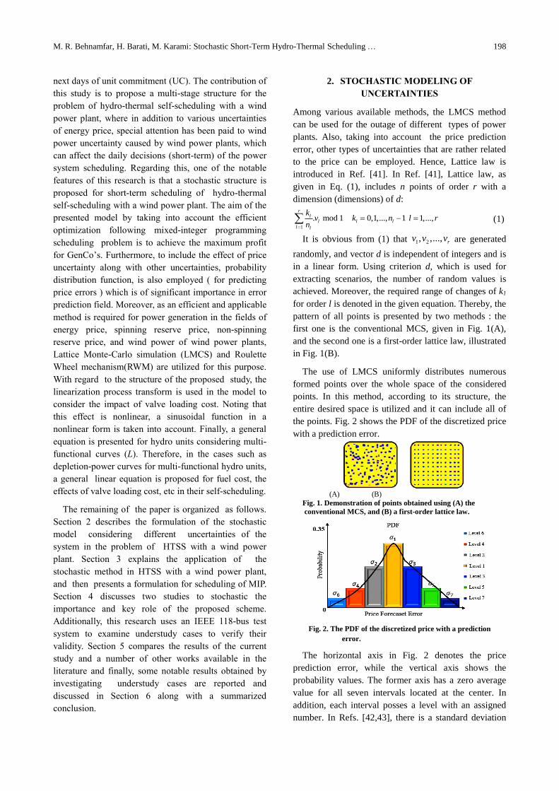
The use of LMCS uniformly distributes numerous

formed points over the whole space of the considered

points. In this method, according to its structure, the

entire desired space is utilized and it can include all of

the points. Fig. 2 shows the PDF of the discretized price

with a prediction error.

(A) (B)

Fig. 1. Demonstration of points obtained using (A) the

conventional MCS, and (B) a first-order lattice law.

Fig. 2. The PDF of the discretized price with a prediction

error.

The horizontal axis in Fig. 2 denotes the price

prediction error, while the vertical axis shows the

probability values. The former axis has a zero average

value for all seven intervals located at the center. In

addition, each interval posses a level with an assigned

number. In Refs. [42,43], there is a standard deviation


for each interval with a price prediction error (σ).

Regarding different price prediction levels and the

obtained probabilities from PDF, RWM is used in Refs.

[43, 44] to form price scenarios for each hour. As seen

in Fig. 3, it includes the range of [0 1] and the use of

desired probabilities along with the normalization

process. As a result, considering the probability range [0

1] for extracting random numbers beside the

normalization of price predictions, RWM can be used.

Finally, using the available method, in addition to

maintaining the uncertainty behavior of the system with

an appropriate approximation, the number of scenarios

will be reduced.

Fig. 3. Different levels of price prediction using RWM along with

considering the normalization probability.

In [42,43], scenario reduction process (Ns number of

scenarios) is used, where weak scenarios or scenarios

with low probability are eliminated. Therefore,

scenarios with high probability are preserved to

participate in the stochastic multi-objective HTSS(MO-

HTSS) problem with a wind power plant. Fig. 4

illustrates a scenario based on stochastic modeling

considering different uncertainties.

3. MIP FORMULATION FOR STOCHASTIC

HTSS

3.1. Maximization of Expected Profit

The first objective function of the stochastic HTSS with

a wind power plant (conventional type) is the

maximization of expected profit ( ) of GenCoʼs and

is expressed as in Eq. (2) and Eq. (3):

1 :max

s

P b b nr

G t t s s

s N

f E p p profit (2)

sp sp

t t s

sr u d ns

i t s t s i t s i t s t s

sr u d ns

s h t s t s h t s h t s t s

h H

i t s i i t s i t s

i I i t s

h h t s

h H

i I

t T

SR N N

profit SR N N

F SDC Y SUC

VLC

SUC I

p

(3)

Start

Input model parameters and initial estimation of

electricity price and wind speed

Roulette Wheel mechanism and Lattice Mont Carlo

Simulation for random Scenario produce (wind speed/price)

Produce Ns 24 hour Scenario 500

Reduce Scenario 20

S=1

S=S+1Perform Stochastic Optimization problem for S th Scenario

Ns>S

No

Yes

Aggregate the Solutions of the Scenario using

Weighted sum Approach

Print the Objective Function Values and

Hydro power,Thermal power,Wind power

Stop

Fig. 4. Flowchart of the modeling presented for considering

different uncertainties based on a stochastic scenario.

Here we tend to discuss the first objective function

attempting to maximize the expected profit (𝐸𝐺𝑃). Hence,

in the section equation, the first objective function

consists of two parts : the first part equals the bilateral

contract for extracting fixed revenue, and the second

part is equal to the sum of the times of each scenario

multiplied by the corresponding revenue. In Ref. [45],

the start-up cost of hydro units (conventional) is

obtained from Eq. (3). The proposed stochastic HTSS

with a wind power plant is comprised of various

equality and inequality constraints and different

uncertainties. One of the important constraints is the

sum of power generated by hydro-thermal

(conventional) and wind units (unconventional), which

are equal to the sum of power traded in the spot market

plus the bilateral contract. This is given in Eq. (4):

,t T s S

b sp

i t s h t s w t s t t s

w Wi I h H

poutpout pout p p

(4)

In Section 3.2 of the paper, other constraints of the

thermal units are described. To provide a relationship

between hydro and wind units it is necessary to

introduce a model for hydro units. Therefore, by

studying Sections 3.3 and 3.4, this issue is addressed.

P

GE


3.2. Model of Thermal Units

It should be noted that as the equations of thermal units

have nonlinear structures they must be transformed into

linear equations. As a result, the equations presented in

Sections 3.2.1, 3.2.2, 3.2.3, 3.2.4 and 3.2.5 for these

units are linearized because of the necessity of solving

the considered problem.

3.2.1. Fuel cost function considering POZs

In thermal units, a quadratic function is assigned to

calculate the fuel cost. Noticing that these units have

special operating conditions, mechanical limitations

such as shaft ball bearing vibration hinder the operation

of such units in some areas that must be separated from

other areas. Fig. 5 shows the linearized form of the fuel

cost function of thermal units, which linear and

piecewise and has M POZs. For this, from a

mathematical point of view, equations (5) and (6) are

ruling for

, ,i I t T s S

1

1

1

( )

M

u n n n

i t s n i i t s i i t s

n

F F p b G (5)

1

1

1

[( ) ]

M

u n n

i t s n i i t s i t s

n

pout p G (6)

Fig. 5. Linearization of the fuel cost function along with M POZs

in a piecewise linear form.

Furthermore, considering that the fuel cost function

of thermal units has variable 0 or 1, only when this

function of power block n and for the i-th thermal unit

will be 1 that the mentioned function is considered in a

piecewise and linear form. The result is that the output

power of the thermal unit is obtained from Eq. (6). In

the rest of the discussion, the fuel cost function of units

can be transformed from a nonlinear to linear form Ref.

[46]. The necessary constraints are given in Eqs. (7-9).

For accurate examination, the maximum 𝑝𝑀+1 𝑖𝑑 = 𝑝𝑖

𝑚𝑎𝑥

and minimum 𝑝𝑜 𝑖𝑢 = 𝑝𝑖

𝑚𝑖𝑛 output power of this plant as

the upper and lower limits are given in Eq. (8).

However, considering constraint (9), the unit which is

definitely operating in the allowed areas is taken into

account.

Fig. 6. Effect of VLC as a pure sinusoidal function which

is transformed into a linear form

0 ; 1,2,..., 1 , ,n

i t sG n M i I t T s S (7)

1[ ] 1,2,..., 1n d u n

i t s n i n i i t sp p G n M (8)

1

1

, ,M

n

i t s h t s

n

I i I t T s S

(9)

3.2.2. Valve loading cost effects

In references [32], [47] and [48], a general case of valve

loading cost function for thermal units is presented,

which is in a completely nonlinear or nonconvex form.

According to Fig. 6 and considering the presented

discussion, it is the effects of Eqs. (10)-(13) on

investigating the effects of VLC are obviously noted. It

is crystal clear that one of the features of function

foam (.) in Eq. (13) is that it rounds its argument to its

closest upper integer value. Take foam (3.1) for

example, where it outputs 4. It is construed from Eq.

(11) that when the necessary power is obtained from

each block of the thermal unit, and the considered unit

with its minimum power participates in cooperation and

scheduling of other units, this power will be equal to the

power produced by 𝑝𝑜𝑢𝑡𝑖 𝑡 𝑠 .

, ,i I t T s S

4 1 4 4

0

4 2 4 3

0

( 2) [ ]2

( )( )

(2 2)

i

i

kn n

i t s i t s

n

i t s i i kn n

i t s i t s

n

VLC e f

(10)

, ,i I t T s S

min 4 1 4 2 4 3 4 4

0

ikn n n n

i t s i i t s i t s i t s i t s i t s

n

pout p I

(11)

, ,i I t T s S

1 1( ) ( )4 4

i t s i t s i t s

i i

If f

(12)

, , 2,3,..., ,ii I t T n x s S

1( ) ( )4 4

n n n

i t s i t s i t s

i if f

(13)

max min

[ ( )]

i ii i

p pk foam f

(13.1)

max min

[4 ( )]i ii

p px foam f

i


The role of the first block given in constraint (12)

states that the output power of the thermal unit is

determined by this block. In fact, a value equal to or

greater than (π/4fi), which corresponds to the first block,

shows the output of thermal units. Now, according to

Eq. (12), it is obvious that when the i-th thermal unit is

trying to generate power, the binary variable 𝐼𝑖 𝑡 𝑠 is used

to prevent the operation of that unit. Referring to Eq.

(12) and Eq. (13), one may notice that the reason behind

using a binary variable 𝜒𝑖 𝑡 𝑠𝑛 is to take into account the

necessary limitation resulting from the generated

power of each block. In other words, the binary variable

will be 1 when 𝑝𝑜𝑢𝑡𝑖 𝑡 𝑠 with respect to block n, has a

higher upper limit. If 𝑝𝑜𝑢𝑡𝑖 𝑡 𝑠 is greater than (𝑛𝜋 4𝑓𝑖⁄ ) +

𝑝𝑖 𝑡 𝑠𝑚𝑖𝑛, the binary variable 𝜒𝑖 𝑡 𝑠

𝑛 will be equal to 1.

3.2.3. Generation capacity limits of the thermal unit

Constraints of the thermal power plant have one lower

and one upper limit. Hence, the mathematical

relationships related to RDL and RUL of the thermal

power plant constraints can be written as Eqs. (14-17). min max

i i t s i t s i t sp I pout pout (14)

max max

1 1 ( )i i t s i t s i t s i i i t sY ip I Y SDR pout (15)

1( )( ) i t s i i i t s i t s i t si YRDL p SDR pout pout (16)

1 1( ) ( ) i i i t s i t s i t s i t si ZSUR RUL p pout pout (17)

3.2.4. Dynamic RDL and RUL

In this section, according to the conducted study in

Ref. [33], it should be said that a function with a DRR is

obtained for power plants. According to condition

∀𝒊𝝐𝑰 , ∀𝒕𝝐𝑻 , ∀𝒔𝝐𝑺 , equations (18) and (19) are

introduced to determine RDL and RUL. 1

1

( )

n n

i t s i t s i

M

n

RDL p RDL (18)

1

1

( )

n n

i t s i t s i

M

n

RUL p RUL (19)

The generated power by thermal units is among those

cases that should be noted and considered in the

calculations shown in Fig.7. It seems that despite the

presence of , thermal units have succeeded to be

associated with DRR through . In addition, the ruling

relationships in these cases are written in Eqs. (18-19).

3.2.5. Other constraints of thermal units

System operators need auxiliary services to provide

safety against events. Reserve services are categorized

into three groups: spinning reserves, non-spinning

reserves in Ref. [48], and alternative or backup reserves.

It should be noted that the reserves are important for

active and reactive powers. In the following, other

constraints given in Refs. [6 and 49] for thermal units

are introduced, which include: startup cost function,

minimum up time (MUT), the minimum down time

(MDT), etc. Moreover, binary variables for scheduling

and cooperation of power plants associated with fuel

limitations are required.

Fig. 7. Generated power in the form of a stepwise function with M

POZs accompanied by limiting the power increment.

3.3. Model of hydro units

Based on Fig.8, a relationship between water depletion,

produced power by hydro units and dam reservoirs of

the upstream units that are in multiple forms, is

established. In general, a model is proposed for hydro

units. Nevertheless, it is worth mentioning that these

units can have a relationship with upstream unitʼs

reservoirs through MIP formulations. To better describe

the mentioned notes, it is concluded from Fig. 8 that

hydro unitʼs are established in parallel, are hydraulically

coupled structures and are related to reservoirs of

upstream hydro units. It is worth sharing that in the

formulation of MIP scheduling problem for hydro units

model, some parameters including power plant dam

reservoirs with small storage volumes, water depletion

oscillations, the output power of the plant, etc are also

presented. Accordingly, the performance curve (L) of

hydro units, given in the formulations, and a number of

upstream units should be accurately considered.

Thereby, the other constraints concerning the hydro

units, which will be mentioned in the following, are

worth noting.

Fig. 8. Hydraulic configuration of the river pool corresponding to

hydro units.


Fig. 9. Performance curves of hydro unit h at time t using piecewise

approximation in a linear form.

3.3.1. Linear formulations for volume and multi-

performance curves

This section of the hydro unit model, as shown in Fig. 9,

includes linear relationships along with performance

curves (L) of hydro units. Equations of this section are

written in Eqs. (20-21). min

h t s hvol vol h H (20)

max 1 max 2 1

1

2

[ ]L

L n n

h L h t s h n h t s h t s h t s

n

vol vol vol

(21)

Performance curves are determined according

to water volume available in dam reservoirs of hydro

units. For this, Eqs. (22-23) can be used.

max 1 2 1 max

1 2

3

[ ]L

L n n

h L h t s h t s h t s h n h t s

n

vol vol vol

(22)

1 2 1.... L

h t s h t s h t s (23)

3.3.2. Linear power discharge performance curves

As mentioned previously, this section discusses the

linearized equations, water depletion of dam reservoirs,

hydro power, and their performance curves (L). Hence,

these equations are given according to Eqs. (24-25). min

1 1

1

[( 1)

] 0 , 1

n n c

h t s h k h t s h t s h k h

n N

k Ln n

h t s h t s

n n k

pout p I Qd b p k

k L

(24)

min

1 1

1

[( 1)

] 0 , 1

n n c

h t s h k h t s h t s h k h

n N

k Ln n

h t s h t s

n n k

pout p I Qd b p k

k L

(25)

3.3.3. Other constraints of hydro units

In summary, we can mention cases like (1) water

overflow from dam reservoirs of hydro units [6], (2)

water balance and the initial volume of water in dam

reservoir of hydro units [6,12], and operation related

services [48].

3.4. Model of wind farms

Wind energy is conceived of as one of the most

important renewable energies. Some benefits of wind

energy include lack of pollution during energy

generation, no need for fuel, low investment cost, to

name but a few. It should be noted that wind sources

change in accordance to their installation site, weather

conditions, and some other parameters. In addition,

wind power plants (unconventional units) have

uncertainties, hence the produced energy by these units

is not highly reliable. To further describe wind turbines,

it is recommended to notice the power produced by such

plants. Fig. 10 shows the use of the power equation for

depicting the curve of output electrical power (kW) of a

wind plant in terms of wind speed (m/s). This is

performed using a simple and usual system which has

succeeded to convert wind energy into electrical energy.

The system is known as wind to electrical converter

system (WECS).

Fig. 10. A simple power-speed curve of a turbine in a wind

power plant.

Focusing on Fig. 10, one may notice that it consists of

different parts : p (kW) is equal to the output power of

the wind plant, pr (kW) is the rated power of the wind

plant. However, other characteristics of the curve in Fig.

10 consist of three velocities : vci , vr , and vco , all in

(m/s). Generally, in this part of the study, a random

value model is used to estimate time series ARMA (n, n-

1), the random velocity of wind to identify the model

and estimate the data [54], we can use equation (26)

where yt is the amount of time series per hour (t).

1

1

1

( )

n

ij

n

t ii j t jty yt

(26)

This equation includes n autoregressive parameters,

n-1 moving average parameters, t is the white noise or

the same prediction error, normal distribution with mean

zero and which represents the standard deviation. In

evaluating the model, coefficients j and i are

calculated and future scenarios are obtained in equation

(26) based on past wind speed data. In the following,

wind speed is calculated using equation (27), where t

represents the mean value.

S = + yt t t tW (27)

Figs. 11 and 12 show the simulated wind speed and

wind power for 20 scenarios in a 24-hour period

obtained by the ARMA model, respectively.

n

h t s


Fig. 11. Wind speed simulated by the ARMA model

Fig. 12. Wind power simulated by the ARMA model

It should be noted that for performing ARMA time

series calculations MINITAB software was used to

reduce the visual scenario of VISUAL STUDIO

programming. Nordex-N80 is a wind turbine model that

has the characteristics of this type of turbines, such as

startup speed, nominal speed, output speed and turbine

capacity, wind -power curve-wind speed, as shown in

Fig. 10. The output power of a wind unit is given in Eq.

(28). In different literature regarding wind turbines, such

as in Refs. [20, 21, 22, 29 and 50], a simple

characteristic is employed to show the relationship

between the input power ( the speed caused by wind )

and the output (electrical) power. Scrutinizing Fig. 10

makes it clear that the generated power of a wind plant

is obtained by Eq. (28).

0P v V or v Voutin

P aV b v V vr in

P p v V vr out r

1( ) , ( )

v ina p b pr r

v v v vr rin in

(28)

Eq. (28) represents the output power of a wind plant

in different speeds. It is obvious that the wind speed can

be a limiting factor for the output power of the plant. If

the sum of generated power from wind energy at places

with a great number of wind units located close to each

other (wind farms) is required, the real generated power

of such units is found from Eq. (29).

. . .WG

t W W WGp p A N (29)

Where, AW represents the whole area covered by wind

units, η is the efficiency of the generator and wind

turbine inverter, and NWG denotes the number of

important generators corresponding to wind turbines.

4. CASE STUDIES

The IEEE 118-bus test system shown in Fig.13 is used

to study the problem of stochastic HTSS with a wind

power plant along with testing the proposed case studies

and approving their validity. The test system includes

54 thermal units with different fuels. Among these units,

there are 10 units with cruel oil fuel, 11 units with gas

fuel, and 33 units with charcoal fuel. In addition, the

data of 8 hydro power plants are extracted from Ref.

[12]. Fig. 14 shows a schematic of a simple scheme for

three different power plants in power systems. This

simple scheme illustrates locations of conventional

(hydro-thermal) and unconventional (wind) power

plants.

Fig. 13. The utilized IEEE 118-bus test system for study and tests

of the proposed scheme.

Fig. 14. A schematic of a simple design related to the location of

conventional and unconventional power plants in a power

system.

GAMS software was used in Ref. [50] to solve

stochastic HTSS problem accompanied by MIP

scheduling and optimization. It is worth noting that in


this study the assumed time for short-term scheduling is

24 hours (one day) and the number of scenarios after

reduction is 20. Also, a personal computer with Intel (R)

core (TM) i3-2370 M CPU @ 2.40 GHz - RAM 4.00

GB, and CPLEX solver from GAMS software are

utilized for simulation purposes. Necessary assumptions

and data for case studies of the research are reported in

this section: (1) It should be said that due to the

availability of required data of ramp rate these data are

assumed as constant values in this study, (2) During

scheduling and cooperation process among units, some

of thermal units, such as 33, 41, 46, and 49 are not

employed because they impose high costs on the

system, (3) In bilateral contract of electricity pricing, it

is necessary to determine the amount and price of

energy for each hour. Therefore, these two values are

assumed to be 1000 MWh and 45 $/MWh, respectively.

(4) A part of hydro unit modeling is comprised of the

relationship between three parameters: the head of water

in the dam reservoir, depleted water from the dam

reservoir, and the generated power. This relationship is

of great importance. Fig. 9 shows that hydro units have

a number of performance curves (L) where each curve

includes a number of blocks, the number of which is 3

and 4. (5) In [51], it is concluded that the amount of fuel

consumption and costs of hydro units will be equal to

the used energy at the startup time. (6) The required data

for scheduling wind units by other generating units is

drawn from [52]. (7) All data of thermal units like POZs

and coefficients of VLC are extracted from [54]. (8) For

scheduling and cooperation of hydro and thermal units,

the required data given in [12, 52] are used. Following

is described the two cases that were utilized for

investigations.

Case 1 addresses the stochastic solution of the HTSS

problem to maximize the profit of GenCoʼs. Hence, this

study aims at investigating the effects of VLC, POZs,

uncertainties of energy price, spinning and non-spinning

reserve prices, without considering the effect of wind

power uncertainty on maximizing the overall profit

expected from hydro-thermal units in the absence of

wind units. It could be expected that the effect of VLC

causes additional costs on thermal plants, changes the

produced power, and reduces the profit of GenCoʼs. In

Case 2, the same conditions of Case 1 are assumed, but

the effect of wind power uncertainty on maximizing the

overall profit expected from hydro-thermal units in the

presence of wind units. It could be expected that the

effect of neglecting the effects of VLC and POZs results

in the increase of profit and limitation of the problem

solving space.

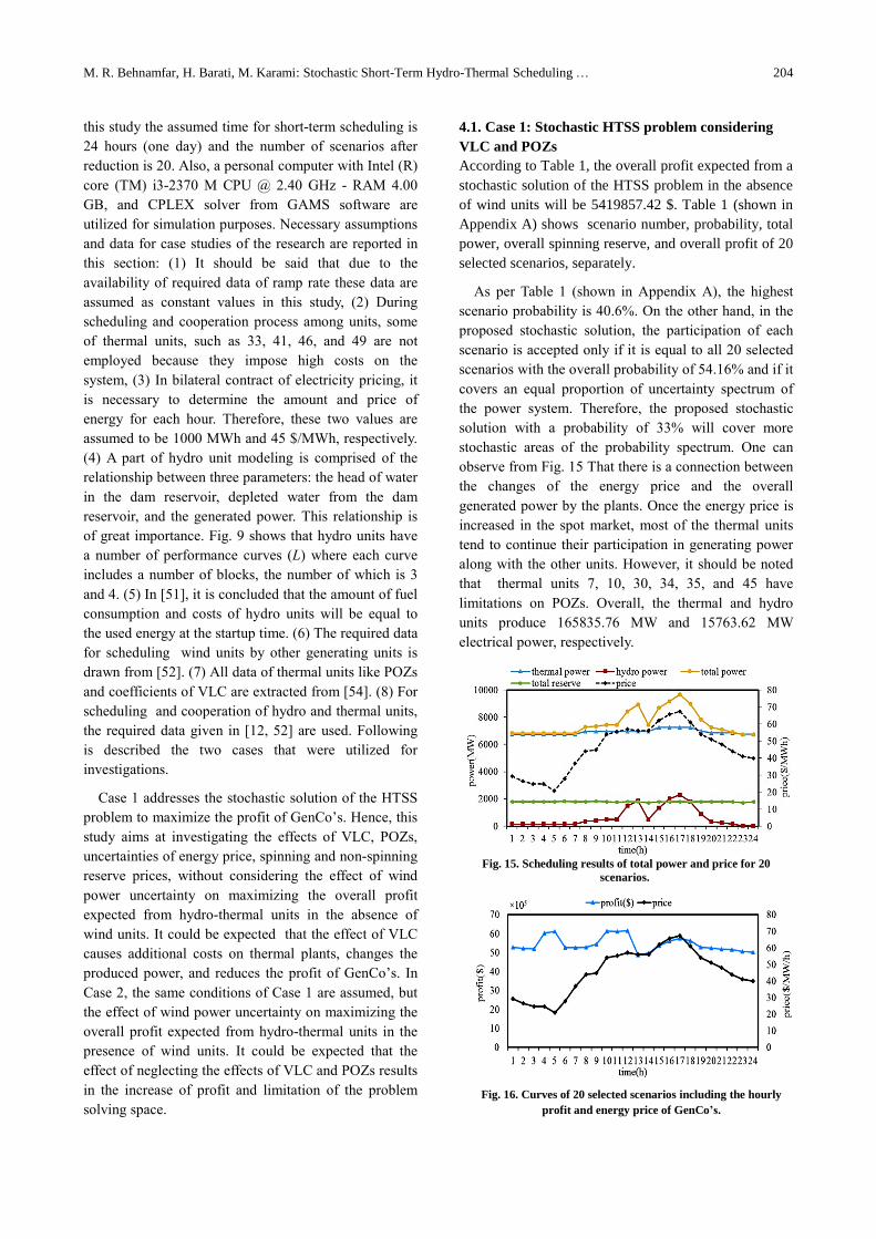
4.1. Case 1: Stochastic HTSS problem considering

VLC and POZs

According to Table 1, the overall profit expected from a

stochastic solution of the HTSS problem in the absence

of wind units will be 5419857.42 $. Table 1 (shown in

Appendix A) shows scenario number, probability, total

power, overall spinning reserve, and overall profit of 20

selected scenarios, separately.

As per Table 1 (shown in Appendix A), the highest

scenario probability is 40.6%. On the other hand, in the

proposed stochastic solution, the participation of each

scenario is accepted only if it is equal to all 20 selected

scenarios with the overall probability of 54.16% and if it

covers an equal proportion of uncertainty spectrum of

the power system. Therefore, the proposed stochastic

solution with a probability of 33% will cover more

stochastic areas of the probability spectrum. One can

observe from Fig. 15 That there is a connection between

the changes of the energy price and the overall

generated power by the plants. Once the energy price is

increased in the spot market, most of the thermal units

tend to continue their participation in generating power

along with the other units. However, it should be noted

that thermal units 7, 10, 30, 34, 35, and 45 have

limitations on POZs. Overall, the thermal and hydro

units produce 165835.76 MW and 15763.62 MW

electrical power, respectively.

Fig. 15. Scheduling results of total power and price for 20

scenarios.

Fig. 16. Curves of 20 selected scenarios including the hourly

profit and energy price of GenCoʼs.


Having this in mind, Fig.16 illustrates how energy

price oscillations can affect 20 selected scenarios related

to the profit of GenCoʼs. Consequently, during hours

13:00 - 21:00, when the energy price increases,

GenCoʼs try to produce much more power and achieve

a considerable amount of profit. Nevertheless, between

hours 1:00 - 13:00 and 21:00 - 24:00 the situation is

completely different. Table 2 (shown in Appendix B)

lists the number of equations, variables, discrete

variables, solution time, and the number of iterations.

4.2. Case 2: Stochastic HTSS problem considering

WP and neglecting VLC and POZs

According to Table 3 (shown in Appendix C), the

overall profit expected from the stochastic solution of

the HTSS problem in the presence of wind units will be

5841292.48 $. Table 3 (shown in Appendix C),shows

scenario number, probability, total power, overall

spinning reserve, and overall profit of 20 selected

scenarios, separately.

Referring to Table 3(shown in Appendix C), the

highest scenario probability is 43.2% . It should be

noted, however, that in the proposed stochastic solution,

the participation of each scenario is accepted only if it is

equal to all 20 selected scenarios with the overall

probability of 56.17% and if it covers an equal

proportion of the power system uncertainty spectrum.

Therefore, the proposed stochastic solution with a

probability of 43.2% will cover more stochastic areas of

the power system probability spectrum. In the

framework of the proposed model for solving the HTSS

problem in the absence of a wind plant, among 500

scenarios generated by LMCS and RWM, only 20

scenarios will remain. Scheduling results of the hydro-

thermal units and the costs related to 20 scenarios are

given in Fig. 17. One can observe from Fig. 17 that

there is a connection between the changes in energy

price and overall generated power of plants. Once the

energy price increases in the spot market, most of the

thermal units tend to continue participation in

generating power along with other units. As a result,

thermal units 3, 33, 46 and 49 that a great amount of

generation cost must be turned off during the scheduling

period. Overall, thermal units produce 166260.17 MW

and the average generation power is 6927.51 MW. The

minimum generated power by thermal units at hour

00:00 is 6855 MW/h. Yet, the maximum generated

power during 16-18 is 7253 MW/h. Variations in the

generated power of thermal units are very small, i.e.

3.6%, and this is because of the range of power changes

of the thermal units. For this reason, thermal units

follow the energy price changes very slowly. On the

other hand , hydro units, during the whole period,

produce 15854.6 MW, where the average power

generation is 656.8 MW/h. The minimum generated

power of hydro units at the hour 24:00 is 23.95 MW and

the maximum generated power at hour 17:00 is 2300

MW. Since the variations in the generated power of

hydro units are very great 73.39%, they can follow

energy price changes in the spot market. At the first

hours of scheduling, water is stored in reservoirs

because energy price is low. However, at middle hours

due to the increase in energy price, the generated power

by hydro units increases as well. Finally, at last hours

and with the decrease in energy price, the produced

power also decreases and water is stored in reservoirs to

meet the constraint of the final volume of the reservoir

water. During the whole scheduling time (24 hours) of

scenario 15, the wind unit produces 3089.49 kW, where

its average is 128.72 kW/h. Since the accurate

prediction of wind speed is impossible, the changes in

the produced power by wind unit are very small 0.28% .

The reason for these small variations is the range of

power changes in the wind unit. Hence, the wind unit

can follow the energy price changes up to a point.

However, Fig. 18 shows how energy price oscillations

can affect 20 selected scenarios related to the profit of

GenCoʼs.

Fig .17. Scheduling results of total power and price for 20

scenarios.

Fig. 18. Curves of 20 selected scenarios that include hourly profit

and energy price of GenCosʼ.


According to 20 selected scenarios, during hours

13:00 - 21:00 the total generated power by hydro-

thermal units in the presence of wind units will change

with a change in the energy price. Consequently, during

this time interval when the energy price is the

maximum, GenCoʼs try to produce more power to

obtain more profit. Nevertheless, between hours 1:00 -

13:00 and 21:00 - 24:00 , the situation is completely

different. Although the calculation procedure of the

proposed method may be time consuming, it seems

that it can be considered a fully reasonable method for

daily decision making.Table 4 (shown in Appendix D )

lists the number of equations, variables, discrete

variables, solution time, and the number of iterations.

In this section, the overall profit expected from solving

the HTSS problem in the presence of wind unit

neglecting VLC and POZs has increased 421435.06 $

compared to Case 1.

5. COMPARATIVE ANALYSIS

In this section, we review references [3, 13, 14 and 15]

by comparing them. Mixed-integer programming (MIP)

for solving the HSS problem only refers to the profit

objective function of GenCoʼs. This article focuses on

three studies, the result of which is the second study,

which is based on the stochastic variable with a profit

value of 938340.178 $ [3].

In Ref. [13], mixed-integer programming for solving

the SCHTC problem refers only to the cost objective

function of independent system operators (ISO). At the

same time, the discussion on profit is not included in

this article.

In Ref. [14], the single-objective profit function is

used to solve the HTSS problem of GenCoʼs, which is

associated with mixed-integer programming. This

article also has three case studies. The profit value of the

third case is 5980401.18 $. Mixed-integer programming

was used to solve the HTSS problem in Ref. [15]. In

addition, the function is multi-objective, which includes

profit and pollution.

However, in our research, using mixed-integer

programming to solve the HTSS and wind power

problem based on the stochastic variable, only one

objective function is used to maximize the profit. The

profit values of the first and second case studies are

5419857.42 $ and 5841292.48 $, respectively. It should

be noted that there are some issues in this study such as

taking into account various types of constraints and

lack of certainties of wind power, energy prices, etc.

which can be used in the discussion on profit, how to

plan and participate effectively in GenCoʼs.

6. CONCLUSIONS

A structure is proposed for the MIP problem in this

study to maximize the GenCoʼs profit, where a

stochastic process is used for the HTSS. Among the

given criteria, considering or neglecting of which may

impact on the study, are fuel limitation, VLC, POZs,

where a linearization method is used to model them.

Furthermore, various uncertainties are assumed for

energy price and wind power.

To achieve a more realistic structure of the considered

HTSS with a wind power plant problem and obtain

more accurate results, one main parameter known as

performance curves (L) of hydro units should be taken

into account. Moreover, in this stochastic HTSS with a

wind power plant problem, different uncertainties with

essential predictions are employed that can be very

effective on maximizing GenCoʼs profit.

Hence, in general, the objective of this study is to

utilize the HTSS with a wind power plant in short-term

(24 hours) scheduling and a stochastic model is

presented that includes different operating constraints

considering/neglecting some other criteria. In addition,

uncertainties associated with energy price prediction,

spinning/non-spinning reserves, and renewable energy

resources like windpower are employed. It was

previously mentioned that the main strategy of GenCoʼs

decision making in simultaneous participation of

conventional (hydro-thermal) and unconventional

(renewable sources like a wind power plant) units and

the use of various scheduling and optimization methods

is to achieve the maximum expected profit.

As a result, the methodology to reach the maximum

expected profit of GenCoʼs is proposed in this paper and

acceptable results are obtained. With regard to the

proposed framework, only 20 out of 500 scenarios

remain indicating a 25% filtering ratio. As a result of

this scenario filtering, more areas are covered by

uncertainties. The advantage of the proposed method is

the increased accuracy and its disadvantage is to select

the filtering ratio.

Then the process and computations times will

increase. The result is that the amount of profit from the

first case, which refers to the stochastic hydro-thermal

self-scheduling (HTSS) regarding VLC, POZs is

5419857.42 $. Profit of the second study i.e. the

stochastic hydro-thermal self-scheduling (HTSS)

without VLC, POZs is 5841292.48 $. The final point is

that GenCoʼs can maximize their profit in the short-

term while generating greater power and providing

better services.


Appendix

Table A. 1. Results of stochastic solving of scenarios in case

study 1 based on HTSS problem

Num

ber

Scen

ario

num

ber

Probability Normalized

probability

Total power

(MW)

Total reserve

(MW) Profit ($)

1 5 0.4063068 0.573 6830 1814 5272942.7

2 15 0.0004821 0.028 6830 1811 5213649.1

3 50 0.0007234 0.033 6830 1811 5199421.8

4 61 0.0060395 0.020 6830 1793 6023951.2

5 100 0.0017311 0.007 6830 1814 6108186.1

6 131 0.0206119 0.008 6830 1796 5258321.6

7 155 0.0045621 0.035 6830 1814 5252624.6

8 178 0.0076238 0.014 7278 1774 5272942.7

9 206 0.0003581 0.008 7338 1814 5452952.6

10 261 0.0403841 0.084 7428 1808 6138442.1

11 274 0.0036746 0.023 7427 1811 6108186.1

12 290 0.0054987 0.025 8427 1795 6158952.1

13 311 0.0035498 0.004 8927 1777 4871240.5

14 350 0.0183591 0.006 7427 1792 4974193.5

15 357 0.0003714 0.035 8675 1814 5361612.8

16 400 0.0000855 0.011 9175 1809 5468491.6

17 419 0.0070981 0.021 9657 1813 5445152.3

18 444 0.0048820 0.003 8975 1813 5433257.7

19 451 0.0019921 0.055 7827 1812 5433257.7

20 472 0.0136728 0.007 7250 1791 5286042.7

Table A. 2. Statistics of optimization results obtained from

solving stochastic HTSS problem. The solver continuously

repeats the iterations to achieve the most appropriate solution

obtained from the final convergence.

HTSS

framwork

Number of

single

equation

Number of

single

variables

Number of

discrete

variables

Number of

discrete

iterations*

Solution

time(Sec)

Stochastic

(case 1) 1345701 1087021 602040 36825 1740

Stochastic

(case 2) 852719 803005 185601 68139 1369

*Number of iterations means the number of iterations that a solver converges

to find the solution.

Table A. 3. Results of stochastic solving scenarios of case study

2 based on HTSS problem N

um

ber

Scen

ario

num

ber

Probability Normalized

probability

Total power

(MW)

Total

reserve

(MW)

Profit ($)

1 2 0.0082613 0.573 6830 1814 5272942.7

2 33 0.0046231 0.028 6830 1811 5213649.1

3 45 0.0001602 0.033 6830 1811 5199421.8

4 59 0.0060510 0.020 6830 1793 6023951.2

5 62 0.0018352 0.007 6830 1814 6108186.1

6 67 0.0066505 0.008 6830 1796 5258321.6

7 84 0.0036497 0.035 6830 1814 5252624.6

8 90 0.0022006 0.014 7278 1774 5272942.7

9 103 0.0036084 0.008 7338 1814 5452952.6

10 116 0.0019720 0.084 7428 1808 6138442.1

11 230 0.0005223 0.023 7683 4009 6140559.5

12 241 0.0045762 0.025 8670 3974 6191594.5

13 283 0.0007503 0.004 9169 3933 6073792.4

14 340 0.0073501 0.006 7664 3967 5191563.7

15 385 0.4320186 0.035 8742 4016 5390029.3

16 392 0.0006214 0.011 9358 4005 6140559.5

17 417 0.0003985 0.021 9638 4013 5393587.6

18 451 0.0184900 0.003 8926 4013 6114807.3

19 480 0.0012030 0.055 7900 4011 5462054.0

20 500 0.0573180 0.007 7520 3965 6163720.9

REFERENCES

[1] M. Shahidehpour, H. Yamin and Z. Li, “Market

operations in electric power systems, forecasting,

scheduling, and risk management”, John Wiley & Sons

Ltd-IEEE Press, New York, 2002.

[2] A. Wood and B. Wollenberg, “Power generation

operation and control”, John Wiley & Sons Ltd, New

York, 2013.

[3] M. Masouleh, et al., “Mixed-integer programming of

stochastic hydro self-scheduling problem in joint energy

and reserves markets,” Electr. Power Compon. Syst., vol.

44, pp. 752-762, 2016.

[4] L. Lakshminarasimman and S. Subramanian, “Short-term

scheduling of hydro-thermal power system with cascaded

reservoirs by using modified differential evolution,”

IEEE. Proc. Gener. Transm. Distrib., vol. 153,pp. 693-

700, 2006.

[5] A. Esmaeily et al., “Evaluating the effectiveness of

mixedinteger linear programming for day-A head hydro-

thermal selfscheduling considering price uncertainty and

forced outage rate,” Energy, vol. 122, pp. 182-193, 2017.

[6] S. Bisanovic, M. Hajro and M. Dlakic, “Hydro-thermal

self-scheduling problem in a day-ahead electricity market

”, Electr. Power Syst. Res. vol. 78, pp.1579-1596, 2008.

[7] M. Shahidehpour and M. Alomoush, “Restructured

electrical power systems, Marcel Dekker”, New York,

2001

[8] M. Giuntoli, “A novel mixed-integer linear algorithm to

generate unit commitment and dispatching scenarios for

reliability test grids”, Inter. Rev. Electr. Eng., vol. 6, pp.

1971-1982, 2011.

[9] Q. Zeng, J. Wang and AL. Liu, “Stochastic optimization

for unit commitment- A review”, IEEE Trans. Power

Syst., vol. 30, 2014.

[10] M. Gavrilas and V. Stahie, “Cascade hydro-power plants

Optimization with honey bee mating optimization

algorithm”, Inter. Rev. Electr. Eng., vol. 6, 2011.

[11] A. Mezger and K. Almeida, “Short-term hydro-thermal

scheduling with bilateral transactions via bundle Method

”, Electr. Power Energy Syst., vol. 29, pp. 387-396, 2007.

[12] A. Conejo, J. Arroyo, J. Contreras and F. Villamor, “Self-

schedulingof a hydro producer in A pool-based electricity

market”, IEEE Trans. Power Syst., vol. 17, pp.1265-

1272, 2002.

[13] M. Karami, H. A. Shayanfar, J. Aghaei and A. Ahmadi,

“Scenario-based security constrained hydro-therm

coordination with volatile wind power generation”,

Renewable Sustain. Energy Rev., vol. 28, pp.726-

737,2013.

[14] J. Aghaei, A. Ahmadi and H. A. Shayanfar and A.

Rabiee, “A Mixed-integer programming of generalized

hydro-Thermal self-scheduling of generating units”,

Electr. Eng., vol. 95, no. 2, pp.109–125,2013.

[15] A. Ahmadi, J. Aghaei, H. A. Shayanfar and A. Rabiee,

“A Mixed-integer programming of multi-objective hydro-

thermal self-scheduling”, Appl. Soft Comput. ,vol. 12,

pp.2137-2146,2012.

[16] UN, “World population prospects”, the 2008 revision

highlights. New York ,United Nations. Department of

Economic and Social Affairs. Population Division , 2009.

[17] D. Connolly, H. Lund, B. Mathiesen and M. Leahy, “A

review of computer tools for analyzing the integration of

renewable energy into various energy systems”, Appl.

Energy., vol. 87, pp.1059-1082, 2010.

[18] A. Foley, P. Leahy, K. Li, E. McKeogh and A. Morrison,

“Along term analysis of pumped hydro storage to firm

http://www.sciencedirect.com/science/article/pii/S0360544217300890

http://www.sciencedirect.com/science/journal/03605442

http://www.sciencedirect.com/science/journal/03605442/122/supp/C


wind power”, Appl Energy. vol. 137, pp. 638-648, 2015.

[19] P. Ilak, I. Rajsl, S. Krajcar and M. Delimar, “The impact

of a wind variable generation on the hydro generation

water shadow price”, Appl. Energy., vol. 154, pp.197-

208, 2015.

[20] K. Wang, X. Luo, L. Wu and X. Liu, “Optimal

coordination of wind-hydro-thermal based on water

complementing wind”, Renew. Energy., vol. 60, pp.169-

178, 2013.

[21] E. Castronuovo and J. Lopes, “On the optimization of the

daily operation of a wind-hydro power plant”, IEEE

Trans. Power Syst., vol. 19 , pp.1599-1606, 2004.

[22] Z. Jianzhong, et al., “Short-term hydro-thermal-wind

complementary scheduling considering uncertainty

ofwind power using an enhanced multi-objective bee

colony optimization algorithm”, Energy Convers.

Manage., vol. 123, pp.116-129, 2016.

[23] H. Pousinho, V. Mendes and J. Catalão, “A risk-averse

optimization model for trading wind energy in a market

environment under uncertainty”, Energy, vol. 36, pp.

4935-4942, 2011.

[24] J. Catalão, H. Pousinho and J. Contreras, “Optimal hydro

scheduling and offering strategies considering price

uncertainty and risk management”, Energy., vol. 37, pp.

237-244, 2012.

[25] L. Wu, M. Shahidehpour and T. Li, “GENCO’s risk-

based maintenance outage scheduling”, IEEE Trans.

Power Syst., vol. 23, pp. 127-136, 2008.

[26] L. Wu, M. Shahidehpour, Z. Li, “GENCOʼs risk-

constrained Hydro-thermal scheduling”, IEEE Trans.

Power Syst. vol. 23, pp.1847-1858, 2008.

[27] C. Tseng and W. Zhu, “Optimal self-scheduling and

bidding strategy of a thermal unit subject to ramp

constraints and price uncertainty”, IET Gener. Transm.

Distrib., vol. 4, pp. 125-137, 2010.

[28] Swedish Energy Agency, “Energy in Sweden 2010, Facts

and Figures”, 2010.

[29] H. Moghimi, A. Ahmadi, A. Aghaei and M. Najafi, “Risk

constrained self-scheduling of hydro-wind units for short

term electricity markets considering intermittency and

uncertainty”, Renewable. Sustain. Energy Rev., vol. 16,

pp. 4734-4743, 2012.

[30] G. Shrestha, S. Kai and L.Goel, “An efficient stochastic

Self-scheduling technique for power producers in the

deregulated power market”, Elect. Power Syst. Res., vol.

71, pp. 91-98, 2004.

[31] M. Li, Y. Li and G. Huang, “An interval fuzzy two-stage

stochastic programming model for planning carbon

dioxid etrading under uncertainty”, Energy, vol. 36, pp.

5677-5689, 2011.

[32] K. Meng, H. Wang, Z. Dong and W. KP, “Quantum

inspired particle swarm optimization for valve point

economic load dispatch”, IEEE Trans. Power Syst., vol.

25, pp. 215-222, 2010.

[33] T. Li and M. Shahidehpour, “Dynamic ramping in unit

commitment”, IEEE Trans. Power Syst., vol. 22,

pp.1379-1381, 2007.

[34] M. Karami, H.A. Shayanfar, J. Aghaei and A. Ahmadi,

“Mixed-integer programming of security-constrained

daily hydro-thermal generation scheduling”, Sci. Iran.

Vol. 20, pp. 2036-2050, 2013.

[35] A. Ahmadi, M. Charwand and J. Aghaei, “Risk-

constrained optimal strategy for retailer forward contract

portfolio”, Int. J. Elect. Power Energy Syst., vol. 53, pp.

704-713, 2013.

[36] H. Wei, et al., “Short-term optimal operation of hydro-

wind-solar hybrid system with Improved generative

adversarial networks”, Appl. Energy, vol. 250, pp. 389-

403, 2019.

[37] G. Díaz, J. Coto and J. Aleixandre, “Optimal operation

value of combined wind power and Energy storage in

multi-stage electricity markets”, Appl. Energy, vol. 235,

pp.1153-1168, 2019.

[38] E. Akbari, R. Hooshmand, M. Gholipour and M.

Parastegari, “Stochastic programming-based optimal

bidding of compressed air energy storage with wind and

thermal generation units in energy and reserve market”,

Energy, vol. 171, pp. 535-546, 2019.

[39] J. Xu, F. Wang, C. Lv, Q. Huang and H. Xie, “Economic-

environmental equilibrium based optimal scheduling

strategy towards wind-Solar-thermal power generation

system under limitedresources”, Appl. Energy, vol. 231,

pp. 355-371, 2018.

[40] S. Zabetian and M. Oloomi, “How does large-scale wind

power generation affect energy and reserve prices”, J.

Oper. Autom. Power Eng., vol. 6, pp.169-182, 2018.

[41] L.Wu, M. Shahidehpour and T. Li, “Stochastic security-

constrained unit commitment”, IEEE Trans. Power Syst.,

vol. 22, pp. 800-811, 2007.

[42] L.Wu, M. Shahidehpour and T. Li, “Cost of reliability

Analysis based on stochastic unit commitment”, IEEE

Trans. Power Syst., vol. 23, pp.1364-1374, 2008.

[43] N.Amjady, J. Aghaei and H. A. Shayanfar, “Stochastic

multi-objective market clearing of joint energy and

reserves auctions ensuring power system security”, IEEE

Trans. Power Syst., vol. 24, pp.1841-1854, 2009.

[44] I. Damousis, A. Bakirtzis and P. Dokopolous, “A solution

to the unit-commitment problem using integer coded

genetic algorithm”, IEEE Trans. Power Syst., vol. 19,

pp.198-205, 2003.

[45] O. Nilsson and D.Sjelvgren, “Hydro unit start-up costs

and their impact on the short-term scheduling strategies

of swedish power producers”, IEEE Trans. Power Syst.

vol.12, pp. 38-44, 1997.

[46] H. Daneshi, A. Choobbari, M. Shahidehpour and Z. Li,

“Mixed-integer programming method to solve security

constrained unit commitment with restricted operating

zone limits”, IEEE Int. Con. EIT., pp.187-192, 2008.

[47] M. AlRashidi and M. El-Hawary, “Hybrid particle swarm

optimization approach for solving the discrete OPF

problemconsidering the valve loading effects”, IEEE

Trans. Power Syst., vol. 22, pp. 2030-2038, 2007.

[48] T. Li and M. Shahidehpour, “Price-based unit

commitment: a case of lagrangian relaxation versus

mixed-integer Programming”, IEEE Trans. Power Syst.,

vol. 20, pp. 2015-2025, 2005.

[49] J. Arroyo and A. Conejo, “Optimal response of a thermal

unit to an electricity spot market”, IEEE Trans. Power

Syst., vol. 15, pp. 1098-1104, 2000.

[50] Generalized Algebraic Modeling Systems (GAMS) ,

[Online] Available: http://www.gams.com

[51] http : / / motor. ece.iit.edu / data / PBUC data . pdf. Also

Market price is from http : / /motor . ece .iit.edu / data

/PBUC data.pdf.

[52] http://motor.ece.iit.edu/data /118bus_abreu. xls.

[53] http://motor.ece.iit.edu/data/118_nonsmooth. xls.

[54] B. Brown, R. Katz and A. Murph, “Timeseries models To

simulateand forecast wind speed and wind power”, J.

Appl. Meteorol., Vol. 23, pp.1184-1195, 1984.

http://ieeexplore.ieee.org/xpl/mostRecentIssue.jsp?punumber=4547422

http://www.gams.com/

http://motor.ece.iit.edu/data

http://motor.ece.iit.edu/data/118_nonsmooth.%20xls

stochastic short-term hydro-thermal scheduling based on

Documents