Stochastic Reward Nets for Reliability Prediction

Jogesh K. MuppalaDept. of Computer Science

The Hong Kong University of

Science and Technology

Clear Water Bay

Kowloon, Hong Kong

Gianfranco CiardoDept. of Computer Science

College of William and Mary

Williamsburg, VA 23187, USA

Kishor S. Trivedi∗

Dept. of Electrical Engineering

Duke University

Durham, NC 27706, USA

Abstract

We describe the use of stochastic Petri nets (SPNs) and stochastic reward nets (SRNs) whichare SPNs augmented with the ability to specify output measures as reward-based functions,for the evaluation of reliability for complex systems. The solution of SRNs involves generationand analysis of the corresponding Markov reward model. The use of SRNs in modelingcomplex systems is illustrated through several interesting examples. We mention the use ofthe Stochastic Petri Net Package (SPNP) for the description and solution of SRN models.

1 Introduction

Combinatorial models such as reliability block diagrams, fault trees and s-t connected net-works are commonly used for system reliability and availability analysis [17, 6]. These modeltypes allow a concise description of the system under study and can be evaluated efficiently,but they cannot represent dependencies occurring in real systems [15, 20], such as imperfectcoverage, correlated failures, repair dependencies, non-zero detection/reconfiguration time,performance-reliability dependence, and phased-mission system models. State space-basedmodels such as Markov models, on the other hand, are capable of capturing various kinds ofdependencies that occur in reliability/availability models [8, 9, 18].

∗This research was sponsored in part by the National Science Foundation under Grant CCR-9108114 andby the Naval Surface Warfare Center.

1

One major drawback of Markov models is the largeness of their state space. The sizes ofthese Markov chains tend to be very large for complex systems. Stochastic Petri nets (SPNs)can be used to generate the (large) underlying Markov chain automatically starting from aconcise description of the system. In such cases the SPN provides a high level interface forthe specification of the underlying Markov model.

In the recent years, SPNs have gained much attention as a useful modeling formalism[1, 4, 16]. They have been successfully used in the analysis of several applications [2, 11, 12].They can easily represent concurrency, synchronization, sequencing and multiple resourcepossession that are characteristics of current computer systems. Several automated toolsthat support the evaluation of SPNs or their variants are available. These include GreatSPN[3], METASAN [16], UltraSAN [7], and SPNP [5].

Traditionally, performance analysis assumes a fault-free system. Reliability and availabil-ity analysis is carried out separately to study system behavior in the presence of componentfaults, disregarding the different performance levels in different configurations. Several differ-ent types of interactions and corresponding tradeoffs have prompted researchers to considercombined evaluation of performance and reliability/availability [13, 19].

Most work on the combined evaluation is based on the extension of Markov chains toMarkov reward models [10], where a reward rate is attached to each state of the Markovchain. Markov reward models have the potential to reflect concurrency, contention, fault-tolerance, and degradable performance; they can be used to obtain not only program/systemperformance and system reliability/availability measures, but also combined measures ofperformance and reliability/availability [13, 19].

As discussed earlier the Markov chain is generated from a concise SPN description ofthe system behavior. In order to facilitate the automatic generation of the Markov rewardmodel, it is necessary to extend the SPN description language to facilitate the specificationof the the reward structure in terms of SPN entities. In other words, the SPN becomes a“SPN reward model” which can be automatically transformed into a Markov reward model.We refer to SPN augmented with the reward description as stochastic reward nets (SRNs)[4].

Steady-state analysis of SRNs is often adequate to study the performance of a system,but time-dependent behavior is sometimes of greater interest: instantaneous availability,interval availability, and reliability (for a fault-tolerant system); response time distributionof a program (for performance evaluation of software); computational availability (for adegradable system). Given the reward rate specification for a Markov reward model, theexpected reward rate is computed in steady-state, while the expected reward rate at time t

is an instantaneous measure of interest. The expected accumulated reward in the interval[0, t) and the expected accumulated reward until absorption are the cumulative measures ofinterest. The mean time to absorption is a special case of the expected accumulated rewarduntil absorption.

The Stochastic Petri Net Package (SPNP) [5] allows the specification of SRN models, thecomputation of steady-state, transient, cumulative, time-averaged, and “up-to-absorption”measures and sensitivities of these measures. Efficient and numerically stable algorithmsemploying sparse matrix techniques are used to solve the underlying CTMC.

In the following sections we give an informal description of SRN and show how it isused in modeling large systems. First, we present a simple example to illustrate some of

2

the structural and reward rate based constructs used in SRNs. Then, we give an informaldescription of SRNs.

2 Stochastic Reward Nets: A Gentle Introduction

In this section, we introduce SRNs through a simple example. Let us consider a simplemultiprocessor system consisting of two dissimilar processors P1 and P2. The time tooccurrence of a failure in the two processors P1 and P2 is assumed to be a random variablewith the corresponding distributions being exponential with rates γ1 and γ2, respectively.The reliability of the two processors at time t is then expressed as R1(t) = e−γ1t and R2(t) =e−γ2t, respectively.

We consider the system to be functioning as long as one of the two processors is function-ing. If we consider the failures of the two processors to be independent, then the reliabilityof this system, Rsys(t) can easily be computed as,

Rsys(t) = 1 − (1 − R1(t))(1 − R2(t))

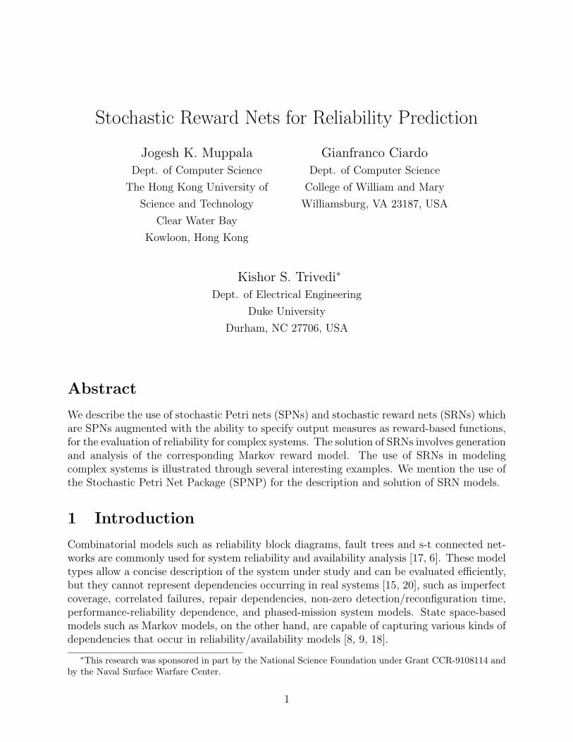
Now suppose that, when both processors are functioning, there is also a a failure modewhere both processors can fail simultaneously. The time to occurrence of this event is alsoassumed to be exponentially distributed with rate γC . Computing the reliability in thissituation is more complicated, because of the failure dependency introduced between thetwo components. Markov models [18] can easily handle such interdependencies as mentionedearlier. The SRN in Figure 1 models the failure behavior of this system.

1P1up 1 P2up

P1dn P2dn

T1fl T2flTcfl

Figure 1: The SRN model of the system

In Figure 1, the main SRN constructs are shown. Places, shown as large circles in thisfigure, represent the various conditions that hold in the system. In this example, the fourplaces, P1up, P2up, P1dn and P2dn represent the conditions in which the processors P1and P2 are up or down, respectively. Transitions, shown in this figure as unfilled rectangles,represent the various events that could occur in the system. In this example, the threetimed transitions, T1fl, T2fl and Tcfl represent the failure of the processors P1, P2 andthe common-mode failure, respectively. We also notice arcs, shown as directional arrows,

3

drawn from places to transitions and from transitions to places. An arc drawn from a placeto a transition is called an input arc into the transition from the place. Conversely, an arcdrawn from a transition to a place is called an output arc from the transition to the place. Wealso notice some small filled dots that are present in the two places P1up and P2up. Theseare called tokens. The presence of a token indicates that the corresponding condition holds.The distribution of tokens in the various places of the SRN is referred to as the marking ofthe SRN.

We consider a transition enabled if each of its input places contains at least one token.An enabled transition may fire removing a token from each of its input places and depositinga token in each of its output places. We know that the events associated with the transitionsabove take a period of time to happen. For example, the time to failure of P1 is known tobe exponentially distributed with rate γ1. This is modeled in the SRN by associating a firing

time with each of the transitions. The firing time (which is a random variable) is the timethat elapses from the time point at which the transition becomes enabled to the time pointat which the transition actually fires. The firing of a transition causes the redistribution ofthe tokens in the SRN, perhaps resulting in a new marking.

1010

1001

0101

0110

T1fl

T2fl T1fl

Tcfl

T2fl

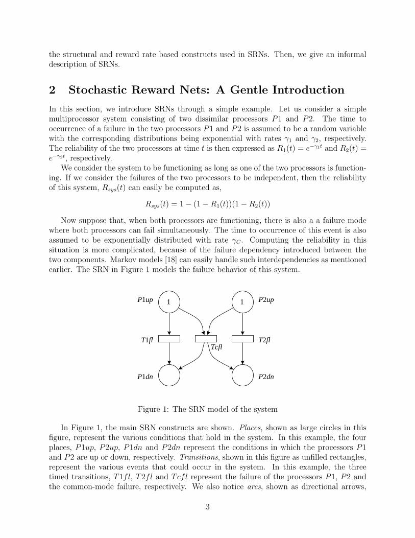
Figure 2: The reachability graph for the SRN

The set of all such markings together with the transitions among them is referred to asthe reachability graph of the SRN. The reachability graph for the example SRN is shown inFigure 2. In this figure, each circle represents a unique marking of the SRN and the elementsof the vector of 0s and 1s given within each circle is the number of tokens in places P1up,P1dn, P2up and P2dn, respectively. The directed arrows show how the system moves fromone marking to another with the firing of the appropriate transition.

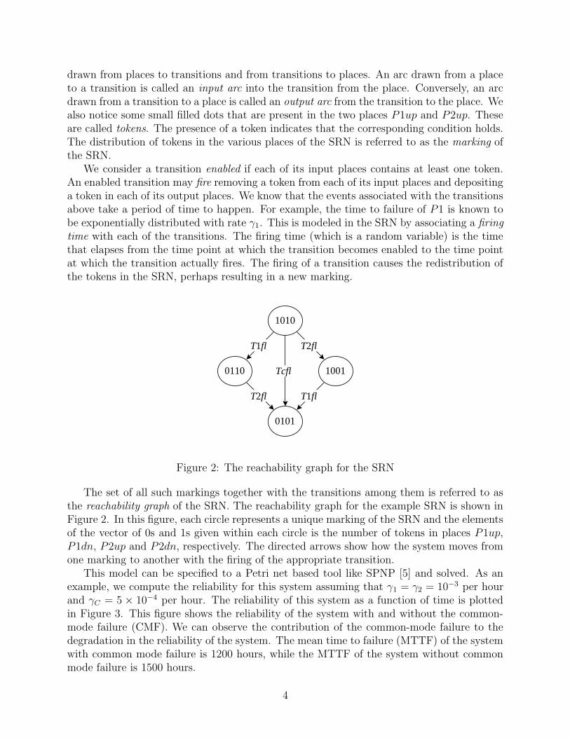
This model can be specified to a Petri net based tool like SPNP [5] and solved. As anexample, we compute the reliability for this system assuming that γ1 = γ2 = 10−3 per hourand γC = 5 × 10−4 per hour. The reliability of this system as a function of time is plottedin Figure 3. This figure shows the reliability of the system with and without the common-mode failure (CMF). We can observe the contribution of the common-mode failure to thedegradation in the reliability of the system. The mean time to failure (MTTF) of the systemwith common mode failure is 1200 hours, while the MTTF of the system without commonmode failure is 1500 hours.

4

0

0.1

0.2

0.3

0.4

0.5

0.6

0.7

0.8

0.9

1

0 2000 4000 6000 8000 10000

R(t)

Time in hours.

With CMF 33

3

3

3

3

3

3

Without CMF +

++

+

+

+

+

++

Figure 3: The reliability for the system

The reliability is computed by assigning appropriate reward rates to the states of theSRN. The reward rates are assigned based on the output measure of interest, in this casethe reliability. We have already seen the various states of the SRN being represented in thereachability graph. Instead of explicitly identifying the states in the reachability graph, wecan specify the reward rates associated with certain conditions of the system. Whenever acondition is satisfied in a state, the corresponding reward rate is assigned to that state.

As an example, in the computation of the reliability of the system, we wish to identifythose states in which the system is functioning, and assign a reward rate of 1 to those states.We will assign a reward rate of 0 to the other states. In the SRN of Figure 1, the system isoperational as long as there exists a token in either of the two places, P1up or P2up. Thusthe reward rate assignment can be specified as follows:

ri =

{

1 if (#(P1up) = 1) ∨ (#(P2up) = 1) in marking i

0 otherwise

Here, ri represents the reward rate assigned to state i of the SRN, and #(p) represents thenumber of tokens in place p. The reliability of the system at time t is computed as theexpected instantaneous reward rate E[X(t)] at time t. Expressions for the computation ofthe expected reward rates are given later in this paper. The MTTF of the system can alsobe computed using the same reward rate assignment as above.

We will introduce more complexity into the example above, by considering state-dependentfailure rates as well as repair of the system. When only one processor is functioning, therate of failure could be correspondingly altered to reflect the fact that a single processorshares the load of both the processors. When only P1 is functioning, we assume its failurerate is γ ′

1and when only P2 is functioning, its failure rate is γ ′

2. We could consider repair of

the processors where the time to repair the processors is also exponentially distributed withrates δ1 and δ2, respectively. We also assume that when both the processors are waiting forrepair, P1 has priority for repair over P2.

5

1P1up 1 P2up

P1dn P2dn

T1fl T2flTcfl

T1rp T2rp

Transition RateT1fl γ1 if #(P2up) = 1

γ′1

otherwiseT2fl γ2 if #(P1up) = 1

γ′2

otherwise

Figure 4: The SRN model of the extended system

The corresponding SRN model, shown in Figure 4, contains two additional transitions,T1rp and T2rp, which represent the repair of the two processors. It also contains a new typeof arc, from P1dn to T2rp, with a small circle instead of an arrowhead: an inhibitor arc. Ifan inhibitor arc exists from a place to a transition, then the transition will not be enabledif the corresponding inhibitor place contains a token. Here, we use the inhibitor arc to givepriority of repair to P1 over P2. The different failure rates of the processors are reflectedby defining the firing rate of the corresponding failure transitions to be a function of themarking of the SRN.

In this case, it makes more sense to talk about the system availability than the systemreliability, since we allow repair from the system failure state. We consider the system to beavailable as long as one of the two processors is functioning. We compute the instantaneousavailability of the system (probability that the system is available at time t) as the expectedinstantaneous reward rate of the system with the same reward rate assignment as used forreliability. The expected interval availability, i.e., the fraction of time the system is availablein the interval [0, t), is given by the time-averaged expected reward rate.

The instantaneous and interval availability for the system is plotted in Figure 5. Weassume γ1 = γ2 = 10−3hr−1, γC = 5.0 × 10−4hr−1, and δ1 = δ2 = 1hr−1 As expected, theinstantaneous and the interval availability decrease with time and reach a steady-state value,which is equal to the steady-state availability of the system.

We can consider one further extension to this model, by considering imperfect coverageof the failure of the processors. Whenever a processor suffers a failure, with some probabilityc, called the coverage probability, the failure is properly detected. With probability 1 − c,the processor suffers an uncovered failure, wherein the failure goes undetected. We assumethat this undetected failure results in the other normal processor also failing, causing the

6

0.9994

0.9995

0.9996

0.9997

0.9998

0.9999

1

0 10 20 30 40 50 60 70 80 90

A(t)

Time in hours.

Inst. Avail. 3

3

33333333 3 3 3 3 3 3 3

Interval Avail. +

+

++++++++

+ + + + + + +

Figure 5: The availability for the system

system failure.This scenario can also be handled by appropriately modifying the earlier SRN model of

the system, resulting in the new SRN model shown in Figure 6.In this figure, there are four new transitions, T1cov, T1uc, T2cov and T2uc, drawn as

thin bars. They are referred to as immediate transitions. Here, T1cov and T1uc representthe covered and uncovered nature of the failure of processor P1, respectively. The other twotransitions T2cov and T2uc represent the same for processor P2. An immediate transitioncan be considered as the limiting case of a timed transition, when the firing rate approachesinfinity. Hence, when enabled, it requires zero time to fire. We associate firing weights withthese transitions. In this model, the weight associated with T1cov and T2cov is c, and theweight associated with T1uc and T2uc is 1 − c, respectively. We also notice two additionalplaces in the figure, namely P1cov and P2cov. These places represent the condition underwhich a decision is being made whether the failure is covered or uncovered. The reachabilitygraph for this SRN is shown in the upper portion of Figure 7, where the order of the placesin the description of the markings is P1up, P1cov, P1dn, P2up, P2cov, and P2dn. Themarkings surrounded by a dotted line are vanishing, that is the SRN does not spend anytime in them, since they enable immediate transitions which fire as soon as they become en-abled. When analyzing the SRN, these markings can be eliminated, resulting in the reducedreachability graph shown in the lower portion of the same figure. Arcs are now labeled withsequences of transitions. For example, it is possible to go from marking 100100 (system com-pletely functional) to marking 001001 (system down) in three ways: by firing transition T1fl

followed by immediate transition T1uc, or transition T2fl followed by immediate transitionT2uc, or transition Tcfl. When the labels are replaced by transition rates, the reducedreachability graph becomes the continuous time Markov chain that is solved to obtain therequested measures.

The availability of the system for different values of the coverage parameter c is plotted in

7

1P1up 1 P2up

P1dn P2dn

T1fl T2fl

Tcfl

T1rp T2rp

T1cov T1uc T2covT2uc

P1cov P2cov

Transition RateT1fl γ1 if #(P2up) = 1

γ′1

otherwiseT2fl γ2 if #(P1up) = 1

γ′2

otherwise

Figure 6: The SRN model of the system with covered and uncovered failures

8

100100

010100

001001

100010

T1fl T2fl

Tcfl

001100 100001

T1cov T2covT1uc T2uc

001010

T2fl T2cov

100001

T1flT1cov

T1rp T2rp

T1rp

100100

001001

(T1fl,T1uc) or Tcfl or(T2fl,T2uc)

001100 100001

T1rp T2rp

T1rp

(T1fl, T1cov)

(T2fl, T2cov)

T2fl,T2cov

T1fl,T1cov

Figure 7: The reachability graph for the system with covered and uncovered failures

9

0.9991

0.9992

0.9993

0.9994

0.9995

0.9996

0.9997

0.9998

0.9999

1

0 10 20 30 40 50 60 70 80 90

A(t)

Time in hours.

c=1.0 3

333333333 3 3 3 3 3 3 3

c=0.9 +

+

++++ + + + + + + +

c=0.8 2

2

Figure 8: The availability for the system with coverage

Figure 8. From the figure we notice that with decreasing coverage probability, the availabilityof the system also correspondingly decreases.

3 Important features of SRNs

In this section, we give a very informal description of the features of SRNs. A formaldescription of SRNs and the numerical algorithms employed to solve the underlying Markovreward models may be found in [4].

3.1 Basic Terminology

A Petri net (PN) is a bipartite directed graph whose nodes are divided into two disjoint setscalled places and transitions. Directed arcs in the graph connect places to transitions (calledinput arcs) and transitions to places (called output arcs). A cardinality may be associatedwith these arcs. A marked Petri net is obtained by associating tokens with places. A marking

of a PN is the distribution of tokens in the places of the PN. In a graphical representationof a PN, places are represented by circles, transitions are represented by bars and the tokensare represented by dots or integers in the places. Input places of a transition are the set ofplaces which are connected to the transition through input arcs. Similarly, output places ofa transition are those places to which output arcs are drawn from the transition.

A transition is considered enabled in the current marking if the number of tokens ineach input place is at least equal to the cardinality of the input arc from that place. Thefiring of a transition is an atomic action in which one or more tokens are removed fromeach input place of the transition and one or more tokens are added to each output placeof the transition, possibly resulting in a new marking of the PN. Upon firing the transition,the number of tokens deposited in each of its output places is equal to the cardinality of

10

the output arc. Each distinct marking of the PN constitutes a separate state of the PN. Amarking is reachable from another marking if there is a sequence of transition firings startingfrom the original marking which results in the new marking. The reachability set (graph) ofa PN is the set (graph) of markings that are reachable from the other markings (connected bythe arcs labeled by the transitions whose firing causes the corresponding change of marking).In any marking of the PN, multiple transitions may be simultaneously enabled.

Another type of arc in a Petri net is the inhibitor arc. An inhibitor arc drawn from aplace to a transition means that the transition cannot fire if the place contains at least asmany tokens as the cardinality of the inhibitor arc.

Extensions to PN have been considered by associating firing times with the transitions.By requiring exponentially distributed firing times, we obtain the stochastic Petri nets. Theunderlying reachability graph of a SPN is isomorphic to a continuous time Markov chain(CTMC). Further generalization of SPNs has been introduced in [1] allowing transitionsto have either zero firing times (immediate transitions) or exponentially distributed firingtimes (timed transitions) giving rise to the generalized stochastic Petri net (GSPN). In thispaper, timed transitions are represented by hollow rectangles while immediate transitionsare represented by thin bars. The markings of a GSPN are classified into two types. Amarking is vanishing if any immediate transition is enabled in the marking. A marking istangible if only timed transitions or no transitions are enabled in the marking. Conflictsamong immediate transitions in a vanishing marking are resolved using a random switch [1].

Although GSPNs provide a useful high-level language for evaluating large systems, repre-sentation of the intricate behavior of such systems often leads to large and complex structureof the GSPN. To alleviate some of these problems, several structural extensions to Petri netsare described in [5] which increase the modeling power of GSPNs. These include guards(enabling functions), general marking dependency, variable cardinality arcs and priorities.Some of these structural constructs are also used in stochastic activity networks (SANs) [16]and GSPNs [3]. Stochastic extensions were also added to GSPNs to permit the specifica-tion of reward rates at the net level, resulting in stochastic reward nets (SRN). All theseextensions are described in the following subsections.

3.2 Marking dependency

Perhaps the most important characteristic of SRNs is the ability to allow extensive markingdependency. Parameters such as the rate of a timed transition, the cardinality of an inputarc, or the reward rate in a marking, can be specified as a function of the number of tokensin some (possibly all) places. Marking dependency can lead to more compact models ofcomplex systems.

3.2.1 Variable cardinality arc

In the standard PN and in most SPN definitions, the cardinality of an arc is a constantinteger value [14]. If the cardinality of the input arc from place p to transition t is k, k

tokens must be in p before t can be enabled and, when t fires, k tokens are removed fromp. Often, all the tokens in p must be moved to some other place q. This behavior can beeasily described in SRNs by specifying the cardinalities of the input arc from p to t and of

11

the output arc from t to q as #(p), the number of tokens in p. This representation is morenatural, no additional transitions or places are required, and the execution time (to generatethe reachability graph) is likely to be shorter.

The use of variable cardinality is somewhat similar to the conditional case construct ofSANs [16]. We allow variable cardinality input, output arcs, and inhibitor arcs.

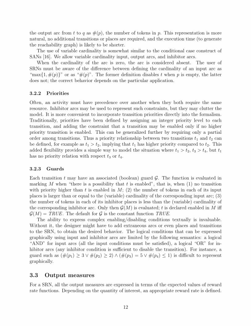
When the cardinality of the arc is zero, the arc is considered absent. The user ofSRNs must be aware of the difference between defining the cardinality of an input arc as“max{1, #(p)}” or as “#(p)”. The former definition disables t when p is empty, the latterdoes not; the correct behavior depends on the particular application.

3.2.2 Priorities

Often, an activity must have precedence over another when they both require the sameresource. Inhibitor arcs may be used to represent such constraints, but they may clutter themodel. It is more convenient to incorporate transition priorities directly into the formalism.Traditionally, priorities have been defined by assigning an integer priority level to eachtransition, and adding the constraint that a transition may be enabled only if no higherpriority transition is enabled. This can be generalized further by requiring only a partialorder among transitions. Thus a priority relationship between two transitions t1 and t2 canbe defined, for example as t1 > t2, implying that t1 has higher priority compared to t2. Thisadded flexibility provides a simple way to model the situation where t1 > t2, t3 > t4, but t1has no priority relation with respect t3 or t4.

3.2.3 Guards

Each transition t may have an associated (boolean) guard G. The function is evaluated inmarking M when “there is a possibility that t is enabled”, that is, when (1) no transitionwith priority higher than t is enabled in M ; (2) the number of tokens in each of its inputplaces is larger than or equal to the (variable) cardinality of the corresponding input arc; (3)the number of tokens in each of its inhibitor places is less than the (variable) cardinality ofthe corresponding inhibitor arc. Only then G(M) is evaluated; t is declared enabled in M iffG(M) = TRUE . The default for G is the constant function TRUE.

The ability to express complex enabling/disabling conditions textually is invaluable.Without it, the designer might have to add extraneous arcs or even places and transitionsto the SRN, to obtain the desired behavior. The logical conditions that can be expressedgraphically using input and inhibitor arcs are limited by the following semantics: a logical“AND” for input arcs (all the input conditions must be satisfied), a logical “OR” for in-hibitor arcs (any inhibitor condition is sufficient to disable the transition). For instance, aguard such as (#(p1) ≥ 3 ∨ #(p2) ≥ 2) ∧ (#(p3) = 5 ∨ #(p4) ≤ 1) is difficult to representgraphically.

3.3 Output measures

For a SRN, all the output measures are expressed in terms of the expected values of rewardrate functions. Depending on the quantity of interest, an appropriate reward rate is defined.

12

Suppose X represents the random variable corresponding to the steady-state rewardrate describing a measure of interest. A general expression for the expected reward rate insteady-state is

E[X] =∑

k∈T

rkπk,

where T is the set of tangible markings (no time is spent in the vanishing markings), πk isthe steady-state probability of (tangible) marking k, and rk is the reward rate in marking k.

Let X(t) represent the random variable corresponding to the instantaneous reward rateof interest. The expression for the expected instantaneous reward rate at time t, becomes:

E[X(t)] =∑

k∈T

rkπk(t),

where πk(t) is the probability of being in marking k at time t.Let Y (t) represent the random variable corresponding to the accumulated reward in the

interval [0, t) and Y represent the corresponding random variable for the accumulated rewarduntil absorption. The expressions for the expected accumulated reward in the interval [0, t)and the expected accumulated reward until absorption are:

E[Y (t)] =∑

k∈T

rk

∫ t

0

πk(x) d x,

andE[Y ] =

∑

k∈T

rk

∫

∞

0

πk(x) d x,

respectively.The computation of the quantities πk, πk(t),

∫ t0πk(x) d x and

∫

∞

0πk(x) d x using numerical

techniques is described in [4].

4 An embedded system

In this section, we use SRNs to model the reliability of an embedded system.

4.1 System description

Consider a system consisting of an input processor, I, connected to three sensors S1, S2,and S3, an output processor O, connected to an actuator with a spare, A1 and A2, a mainprocessor, M , and a bus B (Figure 9).

The input processor polls its three sensors and takes three readings, performs somecomputation on them, such as taking the average or eliminating an outlier, then passes theresult to the main processor. The main processor, in return, elaborates these results intocommands to be passed to the output processor, which controls an actuator.

In a chemical plant environment, the sensor could be reading fluid level, temperature, orpressure, while the actuator could be controlling a valve. In an avionics system, the sensorscould be reading speed, position, or direction, and the actuator could be controlling theflaps.

13

S1

S2

S3

I

A1

A2

OM

Bus

Figure 9: An embedded system.

During the normal operation of the system, the main processor uses a countdown timerto control the frequency at which readings are taken from the input processor and commandsare issued to the output processor. The timer interval is set to τ at the beginning of everycycle.

The reliability of the system is affected by two types of faults. Processors, sensors, andactuators can fail, with rate λp, λs, and λa, respectively (the probability of bus failure isconsidered negligible, hence the bus is not explicitly modeled). The failure of a processoris always fatal. The sensors are used in triple modular redundancy (TMR), using the inputprocessor as the voter, hence the system can survive the failure of one, but not two, sensors.The system is also able to survive the failure of one actuator, since a spare is available. Thesecond type of fault is an intermittent, or transient, fault which might be experienced bythe processors. If an input or output processor experiences a transient fault, it will reboot.During this time, the processor is unavailable, and, if the timer associated with the mainprocessor expires, the system skips one monitoring cycle. A counter is used to keep track ofhow many consecutive cycles have been skipped. If this number exceeds a certain thresholdMaxCount, the main processor decides that at least one of the other two processors hasbeen unavailable for an excessive amount of time, and shuts the system down. We ignorethe possibility of intermittent faults for the main processor, since, if the fault is indeedintermittent, the timer, which is associated with the main processor, can simply stop untilthe reboot is complete. In other words, the main processor must guess the status of theinput and output processors, but not its own. The processor transient failure rate is δf , andthe reboot rate is δr.

4.2 SRN model

The SRN in Figure 10 models the system just described. The meaning of each place andtransition is shown in Table 1. Places DownP , DownS, and DownA are needed only becausewe want to distinguish between the cause of system failure (see Section 4.4). If we were onlyinterested in the probability of the system being up, we could eliminate these places, thusmerging all the absorbing (dead) markings into one, and reducing the size of the underlyingCTMC.

Let’s consider how transition T imer correctly updates the number of tokens in placesStartCycle, EndCycle, and Count. First of all, T imer is always enabled, unless the systemis down. When T imer fires, it removes the token which is either in place StartCycle or

14

1

UpM

FailM

3 2UpS FailS

22

1

UpI FailIBeginTransIEndTransI

TransI

ReadyI

2UpAFailA

1

UpO FailOBeginTransOEndTransO

TransO

ReadyM

1

ComputeI

ComputeO

#(Start)

#(End) if End=0then 1else 0

if End=0then 0else #(Count)

Start

End

ComputeM

Timer

Count

DownP

DownS

DownA

Figure 10: The SRN for the embedded system.

15

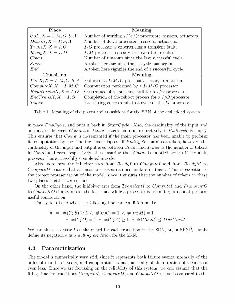
Place Meaning

UpX,X = I,M,O, S,A Number of working I/M/O processors, sensors, actuators.DownX,X = P, S,A Number of down processors, sensors, actuators.TransX,X = I, O I/O processor is experiencing a transient fault.ReadyX,X = I,M I/M processor is ready to forward its results.Count Number of timeouts since the last successful cycle.Start A token here signifies that a cycle has begun.End A token here signifies the end of a successful cycle.

Transition Meaning

FailX,X = I,M,O, S,A Failure of a I/M/O processor, sensor, or actuator.ComputeX,X = I,M,O Computation performed by a I/M/O processor.BeginTransX,X = I, O Occurrence of a transient fault for a I/O processor.EndTransX,X = I, O Completion of the reboot process for a I/O processor.T imer Each firing corresponds to a cycle of the M processor.

Table 1: Meaning of the places and transitions for the SRN of the embedded system.

in place EndCycle, and puts it back in StartCycle. Also, the cardinality of the input andoutput arcs between Count and T imer is zero and one, respectively, if EndCycle is empty.This ensures that Count is incremented if the main processor has been unable to performits computation by the time the timer elapses. If EndCycle contains a token, however, thecardinality of the input and output arcs between Count and T imer is the number of tokensin Count and zero, respectively, thus ensuring that Count is emptied (reset) if the mainprocessor has successfully completed a cycle.

Also, note how the inhibitor arcs from ReadyI to ComputeI and from ReadyM toComputeM ensure that at most one token can accumulate in them. This is essential tothe correct representation of the model, since it ensures that the number of tokens in thesetwo places is either zero or one.

On the other hand, the inhibitor arcs from TransientI to ComputeI and TransientO

to ComputeO simply model the fact that, while a processor is rebooting, it cannot performuseful computation.

The system is up when the following boolean condition holds:

b = #(UpS) ≥ 2 ∧ #(UpI) = 1 ∧ #(UpM) = 1

∧ #(UpO) = 1 ∧ #(UpA) ≥ 1 ∧ #(Count) ≤ MaxCount

We can then associate b as the guard for each transition in the SRN, or, in SPNP, simplydefine its negation b as a halting condition for the SRN.

4.3 Parametrization

The model is numerically very stiff, since it represents both failure events, normally of theorder of months or years, and computation events, normally of the duration of seconds oreven less. Since we are focussing on the reliability of this system, we can assume that thefiring time for transitions ComputeI, ComputeM , and ComputeO is small compared to the

16

Parameter Value Meaning

MaxCount 2 system is down if there are three consecutive timeoutsλp 1/31536000 sec−1 MTTF for a processor is one yearλs 1/2592000 sec−1 MTTF for a sensor is one monthλa 1/5184000 sec−1 MTTF for an actuator is two monthsτ 1/60 sec−1 timeout is one minuteδf 1/86400 sec−1 one transient fault per day per processor, on averageδr 1/30 sec−1 reboot time requires half a minute

Table 2: Parameters for the embedded system.

other activities, hence we can model these three activities with immediate transitions. Thismodification has two advantages: it results in a smaller tangible state space, and it reducesstiffness for the numerical solution. The approximation introduced is negligible, unless thetimeout value τ is similar to the time required to perform the computation, but this wouldnot be reasonable, since the timeout should be set so that it might elapse only when one ofthe processors is rebooting, not during fault-free operation.

The following parameters must then be assigned a value before the SRN can be evaluated:

• MaxCount, the maximum number of timeouts the main processor is willing to acceptbefore deciding that at least one of the other two processors is faulty.

• λp, λs, and λa, the failure rates for the processors, sensors, and actuators, respectively.

• τ , the timeout interval for the main processor.

• δf and δr the transient failure and reboot rates, respectively.

We assume the values given in Table 2.

4.4 Output measures

We are interested in studying the probability that the system has failed by time t, for oneof these possible causes:

• αc = Pr{#(Count) > MaxCount}: the number of consecutive timeouts has exceededMaxCount.

• αp = Pr{#(DownP ) = 1}: one of the processors has failed.

• αs = Pr{#(DownS) = 2}: two sensors have failed.

• αa = Pr{#(DownA) = 2}: both the actuator and the spare have failed.

To compute these probabilities, we can simply define four sets of 0/1 reward rates. Forexample, the reward rate for αc is

ri =

{

1 if #(Count) > MaxCount in marking i

0 otherwise

17

Figure 11 shows the probability of a failure due to the four cases, αc, αp, αs, and αa,computed using SPNP for t = 0, 1, . . . 24 hours and t = 0, 1, . . . 30 days. The reliability isgiven by one minus the sum of these four probabilities. Due to the characteristics of theTMR behavior, and to their low reliability (MTTF is one month), the sensors are the mostcritical components: they account for about 2/3 of the failures. On the other hand, the effectof timeouts is comparable to that of processor failures αc and αp are within a few percent ofeach other, when MaxCount = 2. If the risk of allowing the system to withstand a longersequence of timeouts without shutting down is acceptable, MaxCount could be increased.For example, by doubling its value (MaxCount = 4), αc becomes negligible compared tothe other causes of failure (see Figure 12).

5 Conclusions

In this paper we described the use of stochastic reward nets for the study of reliabilitymodels. Several interesting features of SRNs including marking dependency, guards, variablecardinality arcs and transition priorities were introduced. We also illustrated the specificationof the output measures for the SRN models through the definition of reward rates.

References

[1] M. Ajmone Marsan, G. Conte, and G. Balbo. A class of generalized stochastic Petrinets for the performance evaluation of multiprocessor systems. ACM Trans. Comput.

Syst., 2(2):93–122, May 1984.

[2] M. Ajmone Marsan, S. Donatelli, and F. Neri. GSPN models of multiserver multiqueuesystems. In Proc. Int. Conf. on Petri Nets and Performance Models, pages 19–28,Kyoto, Japan, Dec. 1989. IEEE Computer Society Press.

[3] G. Chiola. A software package for the analysis of generalized stochastic Petri net models.In Proc. Int. Workshop on Timed Petri Nets, pages 136–143, Los Alamitos, CA, July1985. IEEE Computer Society Press.

[4] G. Ciardo, A. Blakemore, P. F. Chimento, J. K. Muppala, and K. S. Trivedi. Automatedgeneration and analysis of Markov reward models using Stochastic Reward Nets. InC. Meyer and R. J. Plemmons, editors, Linear Algebra, Markov Chains, and Queueing

Models, IMA Volumes in Mathematics and its Applications, volume 48. Springer-Verlag,Heidelberg, Germany, 1992.

[5] G. Ciardo, J. Muppala, and K. Trivedi. SPNP: Stochastic Petri net package. In Proc.

Int. Workshop on Petri Nets and Performance Models, pages 142–150, Los Alamitos,CA, Dec. 1989. IEEE Computer Society Press.

[6] C. Colburn. The Combinatorics of Network Reliability. Oxford University Press, NewYork, NY, 1987.

18

0

0.01

0.02

0.03

0.04

0.05

0.06

0.07

0.08

0.09

0.1

0 1 2 3 4 5 6 7 8 9 10 11 12 13 14 15 16 17 18 19 20 21 22 23 24Time (in hours)

αp, αc

αs

αa

0

0.1

0.2

0.3

0.4

0.5

0.6

0.7

0 1 2 3 4 5 6 7 8 9 101112131415161718192021222324252627282930Time (in days)

αp, αc

αs

αa

Figure 11: Failure probabilities αc, αp, αs, and αa during the first day and month of opera-tion.

19

0

0.01

0.02

0.03

0.04

0.05

0.06

0.07

0.08

0.09

0.1

0 1 2 3 4 5 6 7 8 9 10 11 12 13 14 15 16 17 18 19 20 21 22 23 24Time (in hours)

αp

αs

αa

αc

Figure 12: Failure probabilities αc, αp, αs, and αa during the first day of operation whenMaxCount = 4.

[7] J. A. Couvillion, R. Freire, R. Johnson, W. D. Obal II, M. A. Qureshi, M. Rai, W. H.Sanders, and J. E. Tvedt. Performability modeling with ultrasan. IEEE Software,8(5):69–80, Sep. 1991.

[8] J. B. Dugan, K. S. Trivedi, M. K. Smotherman, and R. M. Geist. The Hybrid AutomatedReliability Predictor. AIAA J. Guidance, Control and Dynamics, 9(3):319–331, May-June 1986.

[9] A. Goyal, W. C. Carter, E. de Souza e Silva, S. S. Lavenberg, and K. S. Trivedi.The system availability estimator. In Proc. Sixteenth Int. Symp. on Fault-Tolerant

Computing, pages 84–89, Los Alamitos, CA, July 1986. IEEE Computer Society Press.

[10] R. A. Howard. Dynamic Probabilistic Systems, Vol II: Semi-Markov and Decision Pro-

cesses. John Wiley and Sons, New York, 1971.

[11] O. C. Ibe, K. S. Trivedi, A. Sathaye, and R. C. Howe. Stochastic Petri net modeling ofVAXcluster system availability. In Proc. Int. Workshop on Petri Nets and Performance

Models, pages 112–121, Los Alamitos, CA, Dec. 1989. IEEE Computer Society Press.

[12] S. W. Leu, E. B. Fernandez, and T. Khoshgoftaar. Fault-tolerant software reliabilitymodeling using petri nets. Int. J. Microelectronics and Reliability, 31(4):645–667, 1991.

[13] J. F. Meyer. Performability: A retrospective and some pointers to the future. Perf.

Eval., 14(3-4):139–156, 1992.

[14] J. L. Peterson. Petri Net Theory and the Modeling of Systems. Prentice-Hall, EnglewoodCliffs, NJ, USA, 1981.

20

[15] R. A. Sahner and K. S. Trivedi. Reliability modeling using SHARPE. IEEE Trans.

Reliability, R-36(2):186–193, June 1987.

[16] W. H. Sanders and J. F. Meyer. METASAN: A performability evaluation tool based onstochastic activity networks. In Proc. of the ACM-IEEE Comp. Soc. Fall Joint Comput.

Conf., pages 807–816, Los Alamitos, CA, 1986. IEEE Computer Society Press.

[17] M. L. Shooman. Probabilistic Reliability: An Engineering Approach. McGraw-Hill, NewYork, NY, 1968.

[18] K. S. Trivedi. Probability & Statistics with Reliability, Queueing, and Computer Science

Applications. Prentice-Hall, Englewood Cliffs, NJ, USA, 1982.

[19] K. S. Trivedi, J. K. Muppala, S. P. Woolet, and B. R. Haverkort. Composite performanceand dependability analysis. Perf. Eval., 14(3-4):197–215, 1992.

[20] M. Veeraraghavan and K. S. Trivedi. Hierarchical modeling for reliability and perfor-mance measures. In S. K. Tewksbury, B. W. Dickson, and S. C. Schwartz, editors,Concurrent Computations: Algorithms, Architecture and Technology. Plenum Press,New York, 1987.

21