stochastic programming tools with application to hydropower
TRANSCRIPT

Stochastic Programming Tools withApplication to Hydropower
Production Scheduling
Bachelor’s Thesis
Yves C. Albers
June, 2011
Academic Supervisor:
Professor Thomas F. Rutherford, ETH Zurich
Centre for Energy Policy and Economics
Department of Management, Technology, and Economics


Abstract
This thesis illustrates the framework of stochastic programming as adecision support tool for a hydropower operator. Hydropower plantoperators face uncertain reservoir inflows and electricity spot marketprices. Therefore, they must constantly evaluate the opportunity torelease the available water and produce electricity today against the op-portunity to save the water and sell electricity at a later date in the hopeof more favorable electricity prices. This thesis shows how the opera-tor’s decision process can be modeled as a mathematical optimizationprogram and how to achieve optimization using the General AlgebraicModeling System (GAMS).
This thesis is aimed at undergraduate engineering students with noprior knowledge of GAMS, who should be able to follow the explana-tions with some additional reading of the references listed herein.
The first chapter provides an overview of the main challenges facedby a hydropower operator acting in a liberalized electricity market.GAMS is introduced in a deterministic optimization to find the opti-mal production schedule for a previous year, ex post, assuming that thereservoir inflows and spot market prices are known with certainty.
The second chapter introduces the fundamentals of stochastic recoursemodels to find an optimal reservoir release schedule with respect to un-certain water inflows. Two practical examples are used to illustrate theidea behind two-stage and multi-stage decision models and to demon-strate their implementation with GAMS. The chapter also shows howto model uncertainty with the help of a stochastic scenario tree andprovides two different approaches to describe the structure of such ascenario tree: namely a node-based and a scenario-based notation.
The third chapter focuses on computational issues that arise from largestochastic recourse problems, and shows how to speed up the GAMSmodel generation by introducing a treegeneration tool implemented withthe C++ programming language. The chapter further illustrates howto use a scenario reduction tool within GAMS to reduce the size of amulti-stage model.
The final chapter presents an extended model to find the optimal reser-voir release decision for the following production day, taking into ac-count possible future scenarios of water inflows and spot market pricesduring the following year. The chapter also shows how to incorporaterisk into the model using an expected utility formulation. Finally, thethesis presents some model outcomes based on different input data anddiscusses the results with respect to their effect on the release decisionsand the expected profit.
In this thesis, the Grande-Dixence Dam in the Swiss canton of Valais(a picture of which is shown at the beginning of this thesis [4]) servesas a guideline for the physical reservoir constraints used in the modelspecifications.
iii

Contents
Contents v
1 Introduction 11.1 The Grande-Dixence Hydroelectric Dam . . . . . . . . . . . . 21.2 Liberalized Electricity Market - an Overview . . . . . . . . . . 41.3 Hydropower Release Scheduling . . . . . . . . . . . . . . . . . 61.4 GAMS - The General Algebraic Modeling System . . . . . . . 81.5 Deterministic Release Scheduling . . . . . . . . . . . . . . . . . 9
2 Stochastic Programming 172.1 Two-Stage Pump Storage Example . . . . . . . . . . . . . . . . 182.2 Multi-Stage Problems . . . . . . . . . . . . . . . . . . . . . . . . 222.3 Clear Lake Dam Example . . . . . . . . . . . . . . . . . . . . . 24
2.3.1 Node-Based Notation . . . . . . . . . . . . . . . . . . . 262.3.2 Scenario-Based Notation . . . . . . . . . . . . . . . . . . 30
3 Implementation 373.1 Dynamic Set Assignments . . . . . . . . . . . . . . . . . . . . . 393.2 GAMS Limitations . . . . . . . . . . . . . . . . . . . . . . . . . 423.3 Treegeneration tool . . . . . . . . . . . . . . . . . . . . . . . . . 43
3.3.1 Node-Based Treegeneration . . . . . . . . . . . . . . . . 433.3.2 Scenario-Based Treegeneration . . . . . . . . . . . . . . 443.3.3 Performance of Treegeneration tool . . . . . . . . . . . 46
3.4 Scenario-Reduction . . . . . . . . . . . . . . . . . . . . . . . . . 473.4.1 Performance of SCENRED . . . . . . . . . . . . . . . . 50
3.5 Computational Framework and Model Specification . . . . . . 51
4 Release Model 534.1 Risk aversion . . . . . . . . . . . . . . . . . . . . . . . . . . . . . 584.2 GAMS Implementation . . . . . . . . . . . . . . . . . . . . . . . 60
v
Contents
4.3 Results and Discussion . . . . . . . . . . . . . . . . . . . . . . . 61
A Appendix 69A.1 GAMS Code Clear Lake Node-Based Dynamic Set Assignment 70A.2 GAMS Code Clear Lake Node-Based with treegen.exe . . . . . 72A.3 GAMS Code Clear Lake Scenario-Based with treegen.exe . . . 74A.4 GAMS Code Clear Lake Node-Based with SCENRED . . . . . 76A.5 GAMS Code Release model . . . . . . . . . . . . . . . . . . . . 78A.6 C++ Code Treegeneration tool . . . . . . . . . . . . . . . . . . 82
Bibliography 93
vi

Chapter 1
Introduction
The ongoing liberalization of Europe’s electricity markets has fundamen-tally changed the managerial challenges facing Swiss hydropower produc-tion. The opening up of the markets has caused the energy sector’s politicaland economic reality to shift from a state-dominated, monopolistic systemtowards a market-driven and transnational environment.
In a conventionally regulated market with fixed electricity prices, the opera-tor’s main purpose was to minimize costs and guarantee security of supply.The old system sought to maximize social surplus, whereas the objective inthe present environment is to maximize profits. In view of the reservoir’sphysical constraints and the uncertain evolution of future electricity pricesand water inflows, determining an optimal release schedule has become a chal-lenging optimization task. Based on the available turbine power, dischargecapacities, and inflow forecasts, an operator must constantly decide whetherto generate electricity today or save the water in the hope of more favorableprices.
This chapter outlines the crucial questions faced by a profit-seeking hydro-electric plant operator. The chapter shows how to use GAMS, an algebraicmodeling language applied in large-scale stochastic optimization to deter-mine the optimal release schedule ex post, given that the previous year’selectricity prices and reservoir inflows are known.
The chapter briefly describes the Grand-Dixence hydropower system in theSwiss canton of Valais and uses the technical dimensions of the Grande-Dixence Dam as a reference for the optimization models in this thesis.
1

1. Introduction
1.1 The Grande-Dixence Hydroelectric Dam
Hydropower systems like the Grande-Dixence Dam offer a unique opportu-nity to efficiently store vast amounts of energy. The dam weighs 15 milliontones and withholds the enormous water masses of Lake Dix, which cancontain up to 400 million m3 of water.
Figure 1.1: Gravity Dam
From an engineering point of view, theGrande-Dixence Dam is a typical exampleof a gravity dam that holds back the thrustof the water masses solely with its ownweight. Figure 1.1 shows a schematic trian-gular cross-section, where the broad base-ment becomes narrower as it approachesthe top [4].
Lake Dix is an artificially formed reservoirthat collects the water from a 357 km2-widecatchment area that includes 35 glaciers.Perhaps the most remarkable thing aboutGrande-Dixence is that only about 40 per-cent of the water inflows find their wayto the reservoir by following the naturalgradient. The remaining 60 percent arecollected by a cleverly devised pipeworkand pumping system that includes a 24-kilometer main water conduit.
Four pumping stations can be used to trans-port water from surrounding reservoirs to Lake Dix, which lies at 2364 me-ters above sea level: Z’Mutt, Stafel, Ferpe and Arolla. These reservoirs havea combined capacity of 186 MW of pumping power.
In order to exploit the enormous potential of the stored water masses, fourpower plants are either directly or indirectly linked to Lake Dix: Fionnay,with a turbine capacity of 290 MW: Chandoline, with a turbine capacity of150 MW: Bieudron, with a turbine capacity of 1269 MW: and Nendaz, witha turbine capacity of 390 MW.
Together these four power plants have an installed capacity of over 2000 MW,which is roughly twice the capacity of a medium-sized nuclear power plant,such as Goesgen in Switzerland. The diagram on the next page illustratesthe key elements of the Grande-Dixence system [4].
2


1. Introduction
1.2 Liberalized Electricity Market - an Overview
The difference between electricity and other commodities is that electricitycannot be stored directly as a physical good. Furthermore, in order to main-tain a stable and secure supply, the frequency of the electricity grid mustbe kept at 50 Hertz. Essentially, this means that electricity consumption de-mand must be instantaneously met by production. The fundamental prob-lem is that it is impossible to accurately predict electricity demand becauseit depends on several different factors, such as the prevailing weather con-ditions or the time of day. In addition, electricity demand is rather inelasticin the short-run, as the responsiveness of residential consumption to pricechanges is relatively low.
To ensure a constant grid frequency, sophisticated regulating mechanismshelp to balance the grid load (consumption) and the electricity infeed (pro-duction). In Switzerland, the transmission net operator (TSO) Swissgrid co-ordinates the matching of supply and demand.
Even though electricity cannot be stored directly, hydroelectric dams offeran efficient way to store potential energy. The high operational flexibility ofsuch dams allows the output of generated electricity to be easily adaptedwithin a few minutes, at almost zero marginal costs. Compared to otherenergy sources, such as nuclear energy (which have limited output changes)or gas plants (which have relatively high marginal costs) hydroelectric powerprovides a unique opportunity to meet short-time demand fluctuations.
A hydropower operator can sell his production through one of the followingthree channels:
• The Spot Market
• The Financial Market
• The OTC Market
The Swiss spot market SWISSIX at the EEX1 is a day-ahead market whereelectricity can be traded for each of the 24 hours of the following day. Buyersand sellers can enter their bids electronically. The system matches supplyand demand and calculates a market clearing price for each hour. Duringthe delivery day, each supplier is required to feed-in the exact amount ofelectricity he committed to. Likewise the buyer is required to consume ex-actly the amount of energy he bought the previous day.
In the financial market, participants can trade standardized contracts througha common platform. A futures contract is an agreement between two partiesto exchange a certain amount of electricity at a predetermined price at a
1European Electricity Exchange: The leading energy exchange for the German, Swiss,French, and Austrian markets.
4

1.2. Liberalized Electricity Market - an Overview
future date. Each futures contract has its specific runtime and delivery vol-ume, which is usually 1 MW. The party that agrees to buy the electricityhas the long position. The other party, which agrees to deliver the electric-ity, enters the short position. The EEX offers standardized futures products,which mature on a weekly, monthly, quarterly and yearly basis. An impor-tant feature of the financial market is that it allows participants to settle theircontracts not only on a physical level but also on a purely financial level. Ifthe participants opt for physical delivery, the underlying energy of the fu-tures contracts must be fed into the grid. On the other hand, a financialfutures contract does not involve any physical electricity flows between thetwo parties.
A financially settled contract requires the parties to exchange cash flows inorder to compensate each other for the difference between the agreed deliv-ery price and the actual spot market price during the contractual runtime.
Most electricity exchanges also allow the trading of standardized option con-tracts. A buyer of a European call option has the right, but not the obligationto buy a certain amount of electricity at a predetermined date and strikeprice. Conversely, a buyer of a European put option has the right, but not theobligation, to buy a certain amount of electricity at a predetermined dateand strike price. The buyer of an option must always pay a risk-premium tothe seller.
Finally, the operator can sell his production directly to his clients on a bi-lateral basis. The OTC market2 allows for tailor-made delivery contracts be-tween the supplier and his customers, including full requirement contractsand swing-options.3 Compared to the financial market, the increased flexi-bility of the OTC market involves an increased counterparty and liquidityrisk.
2OTC stands for over-the-counter.3A full requirement contract allows the buyer to obtain as much electricity as it needs,
for a fixed price. A swing-option allows the buyer to obtain electricity within certain volumelimits for a fixed price.
5

1. Introduction
1.3 Hydropower Release Scheduling
From an engineer’s perspective, managing a multi-reservoir system likeGrande-Dixence is a challenging control task. A thorough understanding ofthe system’s physical dynamics, especially of the interdependencies amongthe different reservoirs, pumping stations, and power plants, is vital in orderto control the water flows. In addition to the technical control, the main en-trepreneurial challenge in a liberalized market is to find an optimal release ordischarge schedule that maximizes the value of the available water resources.Basically, the operator must answer the following question:
How much electricity should I produce during each hour of the day in order tomaximize profits?
Stated another way: What is the optimal amount of water to release, in order toget the highest possible value for the stored water?
The difficult part of answering this question is handling the uncertainty ofwater inflows and electricity spot market prices. A producer would naturallyhope to sell electricity during peak hours when energy demand and pricesare relatively high. However, without knowing the prospective prices andinflows, the operator must decide whether to release water today or waitand save the water in the hope of more favorable prices.
In general, yearly demand for electricity reaches a maximum during thecold winter months, when there is an increased need for heating and electriclightning. Therefore, a basic strategy with which to approach the optimalscheduling question would be to save water during summer and maximizeelectricity production during winter.
However, electricity market prices may fluctuate considerably during thecourse of a year depending on various factors, such as the availability ofother production resources and the current state of the economy. If accu-rately predicted, a volatile market situation can offer a lucrative income po-tential.
Therefore, to determine the optimal release moments, which maximize thereservoir’s water value, the operator needs a fundamental understanding ofthe prospective market dynamics.
Statistical models are used to develop price forecasts that represent the basicguideline for the release scheduling decision. Additionally, reservoir inflowsare estimated to get an idea about the available generation resources.
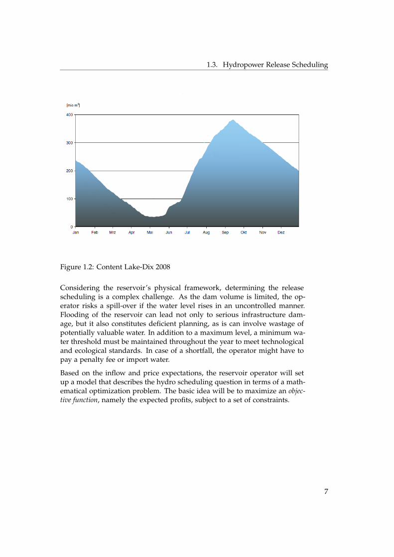
Figure 1.2 [4] shows the evolution of the water level of Lake Dix in 2008. Thehydrological pattern is typical for a reservoir in Switzerland. The dam fillsup during snowmelt in the mild summer months and reaches its maximumcharge by the middle of September. During winter, there is almost no inflowand the dam gradually empties until the end of spring.
6
1.3. Hydropower Release Scheduling
Figure 1.2: Content Lake-Dix 2008
Considering the reservoir’s physical framework, determining the releasescheduling is a complex challenge. As the dam volume is limited, the op-erator risks a spill-over if the water level rises in an uncontrolled manner.Flooding of the reservoir can lead not only to serious infrastructure dam-age, but it also constitutes deficient planning, as is can involve wastage ofpotentially valuable water. In addition to a maximum level, a minimum wa-ter threshold must be maintained throughout the year to meet technologicaland ecological standards. In case of a shortfall, the operator might have topay a penalty fee or import water.
Based on the inflow and price expectations, the reservoir operator will setup a model that describes the hydro scheduling question in terms of a math-ematical optimization problem. The basic idea will be to maximize an objec-tive function, namely the expected profits, subject to a set of constraints.
7

1. Introduction
1.4 GAMS - The General Algebraic Modeling System
GAMS is an algebraic modeling language (AML). This high-level compu-tational framework allows the user to solve large-scale optimization prob-lems. Compared to traditional programming languages like C++ or FOR-TRAN, which require the user to deal with memory allocation and datatypes, AML’s provide a clear and simple algebraic syntax.
The way a problem is formulated within GAMS is very similar to the mathe-matical description of an optimization problem, which makes the handlingof GAMS rather intuitive. The first step is for the user to write down his orher model specifications. The system then interprets the model and calls anappropriate solver to handle the problem. GAMS is linked to a set of vari-ous powerful solvers that can deal with linear, nonlinear, and mixed-integeroptimization problems.
GAMS models are easily portable between different computer platforms.The basic composition of a model specification is given below.
1. Definition and assignment of sets
2. Specification of parameters and assignment of values.
3. Declaration of model variables
4. Definition and declaration of model equations
5. Solve instructions
6. Report generation (typically with the help of an Excel or Matlab inter-face)
Depending on the solve instructions, GAMS produces a comprehensive so-lution report that contains all relevant model information and results. Asthe next example shows, a GAMS code is almost self-explanatory.
8
1.5. Deterministic Release Scheduling
1.5 Deterministic Release Scheduling
This section demonstrates the use of GAMS to find the optimal monthly re-lease schedule for 2008. The optimization becomes a deterministic problemas all involved coefficients are known with certainty. Based on the spot mar-ket prices and reservoir inflows, the aim is to determine the optimal releaseschedule for 2008 that would have maximized profits. Note that this modelonly considers sales on the spot market.
Given the optimal release schedule for 2008, it can be compared to the ac-tually performed schedule in order to find out how much more could havegained if we had had perfect information about the future.
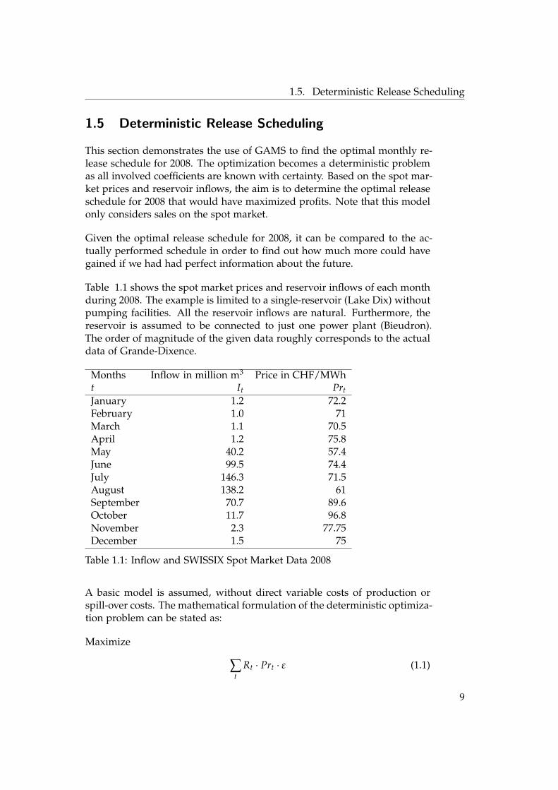
Table 1.1 shows the spot market prices and reservoir inflows of each monthduring 2008. The example is limited to a single-reservoir (Lake Dix) withoutpumping facilities. All the reservoir inflows are natural. Furthermore, thereservoir is assumed to be connected to just one power plant (Bieudron).The order of magnitude of the given data roughly corresponds to the actualdata of Grande-Dixence.
Months Inflow in million m3 Price in CHF/MWht It PrtJanuary 1.2 72.2February 1.0 71March 1.1 70.5April 1.2 75.8May 40.2 57.4June 99.5 74.4July 146.3 71.5August 138.2 61September 70.7 89.6October 11.7 96.8November 2.3 77.75December 1.5 75
Table 1.1: Inflow and SWISSIX Spot Market Data 2008
A basic model is assumed, without direct variable costs of production orspill-over costs. The mathematical formulation of the deterministic optimiza-tion problem can be stated as:
Maximize
∑t
Rt · Prt · ε (1.1)
9

1. Introduction
Subject to
Lt = Lt−1 + It − Rt − St (1.2)Ldec2007 = Lstart (1.3)
Lmin ≤ Lt ≤ Lmax (1.4)0 ≤ Rt ≤ Rmax (1.5)
0 ≤ St (1.6)
Rt represents the amount of water released during month t, Lt is the amountof water stored in the dam at the end of month t, and St is the amount ofwater spilled over during month t. It is the monthly inflow as described inTable 1.1.
Equation 1.1 describes the profit function to be maximized. The total profitis given by the sum of the monthly profits, whereas the monthly profit isgiven by the amount of electricity produced multiplied by the monthly av-eraged spot market price. Equation 1.2 describes the physical balance of ahydropower reservoir without pumping facilities. Constraints 1.3-1.6 repre-sent the boundary conditions of the optimization and are explained in Table1.2.
Notation: Description: Value:Lmax : Maximum water level the dam can store 400 million m3
Lmin : Minimum water level that must be main-tained in the lake
40 million m3
Lstart : Water level at the beginning of the opti-mization horizon (end of December 2007)
200 m3
Rmax : Maximum amount that can be releasedper month
140 m3
ε: Amount of energy (MWh) that can beproduced per amount of water
4618 MWh/mil-lion of m3
Table 1.2: Physical Constraints
Note that no target-reservoir level Lend has been specified for the end of themodel horizon. With respect to the definition of the profit function, this willlead the solution of our optimization to release the whole reservoir by theend of the year. In reality, however, this may be undesirable because theoperational horizon never really ends. It would be unwise to fully releasethe reservoir by the end of the year if high prices were expected for thesubsequent year.
In a more practical setting, in order to avoid so-called end-horizon effects, itwould make sense to constrain the end-horizon level Lend or to extend the
10
1.5. Deterministic Release Scheduling
profit function with a term V(Lend) that accounts for the potential futurevalue of water at the end of the model horizon.
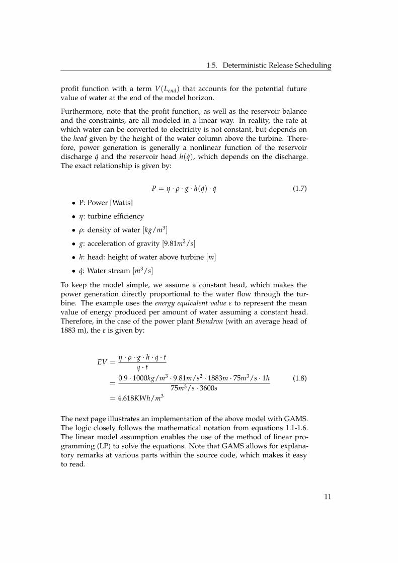
Furthermore, note that the profit function, as well as the reservoir balanceand the constraints, are all modeled in a linear way. In reality, the rate atwhich water can be converted to electricity is not constant, but depends onthe head given by the height of the water column above the turbine. There-fore, power generation is generally a nonlinear function of the reservoirdischarge q̇ and the reservoir head h(q̇), which depends on the discharge.The exact relationship is given by:
P = η · ρ · g · h(q̇) · q̇ (1.7)
• P: Power [Watts]
• η: turbine efficiency
• ρ: density of water [kg/m3]
• g: acceleration of gravity [9.81m2/s]
• h: head: height of water above turbine [m]
• q̇: Water stream [m3/s]
To keep the model simple, we assume a constant head, which makes thepower generation directly proportional to the water flow through the tur-bine. The example uses the energy equivalent value ε to represent the meanvalue of energy produced per amount of water assuming a constant head.Therefore, in the case of the power plant Bieudron (with an average head of1883 m), the ε is given by:
EV =η · ρ · g · h · q̇ · t
q̇ · t
=0.9 · 1000kg/m3 · 9.81m/s2 · 1883m · 75m3/s · 1h
75m3/s · 3600s= 4.618KWh/m3
(1.8)
The next page illustrates an implementation of the above model with GAMS.The logic closely follows the mathematical notation from equations 1.1-1.6.The linear model assumption enables the use of the method of linear pro-gramming (LP) to solve the equations. Note that GAMS allows for explana-tory remarks at various parts within the source code, which makes it easyto read.
11

1. Introduction
1 $title Deterministic, Single Reservoir Water Dispatch Model
2 set t Months /dec2007,jan,feb,mar,apr,may,jun,jul,aug,sep,oct,nov,dec/
3 baset(t) Base Month /dec2007/;
4 *-------------------------------------------------------------------------------
5 parameters i(t) Inflow in time period t
6 / jan 1.2, feb 1.0, mar 1.1,
7 apr 1.2, may 40.2, jun 99.5
8 jul 146.3, aug 138.2, sep 70.7
9 oct 11.7, nov 2.3, dec 1.5/
10
11 p(t) Electricity price in period t quoted in CHF per MWh
12 / jan 72.2, feb 71, mar 70.5
13 apr 75.8, may 57.4, jun 74.4
14 jul 71.5, aug 61, sep 89.6
15 oct 96.8, nov 77.75, dec 75/
16
17 l_min Lower bound on reservoir level /40/,
18 l_max Upper bound on reservoir level /400/,
19 r_max Max release capacity per month in m^3 mio /140/,
20 e Energy equivalent: MWh per million of m^3 /4618/,
21 l_start Water in dam at beginning of the year /200/;
22 *-------------------------------------------------------------------------------
23 variables L(t) Reservoir volume at the end of period t in million m^3,
24 R(t) Water release during period t in million m^3,
25 S(t) Water spill during period t in million m^3,
26 OBJ Objective (revenue);
27 L.lo(t) = l_min;
28 L.up(t) = l_max;
29 L.fx(baset) = l_start;
30 *-------------------------------------------------------------------------------
31 equations level(t) Reservoir level at the end of period t
32 objdef Definition of revenue;
33
34 level(t+1).. L(t+1) =e= L(t) + i(t+1) - R(t+1) - S(t+1);
35 objdef.. OBJ =e= sum(t, p(t)*R(t)* e);
36 R.lo(t) = 0;
37 R.up(t) = r_max;
38 S.lo(t) = 0;
39 *-------------------------------------------------------------------------------
40 model waterplanning /objdef, level/;
41 solve waterplanning using lp maximizing OBJ;
42
12

1.5. Deterministic Release Scheduling
Sets
set t Months /dec2007,jan,feb,mar,apr,may,jun,jul,aug,sep,oct,nov,dec/
baset(t) Base months /dec2007/;
Declare a set named t and assign the set elements {dec2007, jan, f eb, ...}. Thedeclaration is followed by a description of the set (here, Months). The setbaset(t) is a subset of set t and contains one element, namely dec2007, whichrepresents December of the previous year. The set base(t) is used later todefine the initial reservoir level at the beginning of the optimization horizon.
Parameters
parameters i(t) Inflow in time period t
/ jan 1.2, feb 1.0, mar 1.1,
apr 1.2, may 40.2, jun 99.5
jul 146.3, aug 138.2, sep 70.7
oct 11.7, nov 2.3, dec 1.5/
p(t) Electricity price in period t quoted in CHF per MWh
/ jan 72.2, feb 71, mar 70.5
apr 75.8, may 57.4, jun 74.4
jul 71.5, aug 61, sep 89.6
oct 96.8, nov 77.75, dec 75/
Declare an inflow parameter i(t), which depends on set t. Add values to theinflow parameter. Declare a price parameter pr(t), which depends on set t.Add values to the price parameter. These declarations correspond to Table1.1.
Variables
variables L(t) Reservoir volume at the start of period t in million m^3,
R(t) Water release during period t in million m^3,
S(t) Water spill during period t in million m^3,
OBJ Objective (revenue);
L.lo(t) = l_min;
L.up(t) = l_max;
L.fx(baset) = l_start;
Declare the decision variables L(t), R(t) and S(t) for each member of theset t. Declare an objective variable OBJ without any index. L.lo(t) = l minand L.up(t) = l max define a minimum/maximum value for the decisionvariable L(t) for all elements of the set t. L. f x(baset) = l start assigns afix start value to the decision variable L(′dec2007′), which was previouslydeclared in the set baset(t).
13
1. Introduction
Equations
equations level(t) Resevoir level at the start of period t
objdef Definition of revenue;
level(t+1).. L(t+1) =e= L(t) + i(t+1) - R(t+1) - S(t+1);
objdef.. OBJ =e= sum(t, pr(t)*R(t)* EV);
R.lo(t) = 0;
R.up(t) = r_max;
S.lo(t) = 0;
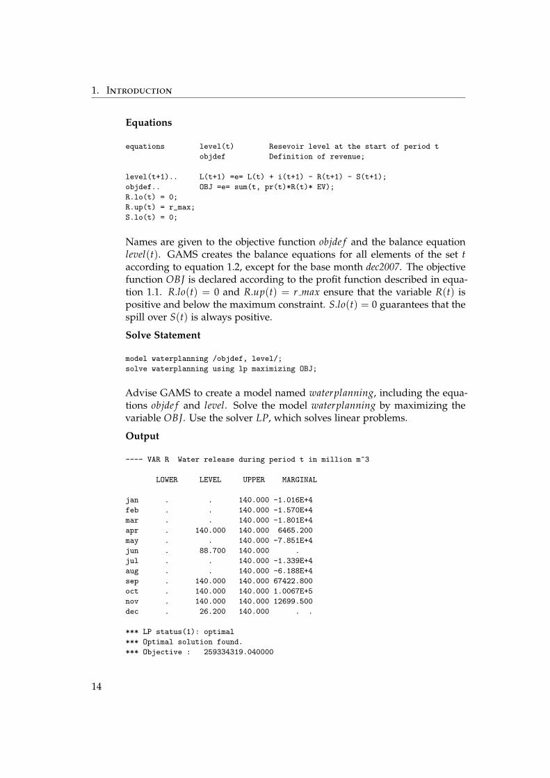
Names are given to the objective function objde f and the balance equationlevel(t). GAMS creates the balance equations for all elements of the set taccording to equation 1.2, except for the base month dec2007. The objectivefunction OBJ is declared according to the profit function described in equa-tion 1.1. R.lo(t) = 0 and R.up(t) = r max ensure that the variable R(t) ispositive and below the maximum constraint. S.lo(t) = 0 guarantees that thespill over S(t) is always positive.
Solve Statement
model waterplanning /objdef, level/;
solve waterplanning using lp maximizing OBJ;
Advise GAMS to create a model named waterplanning, including the equa-tions objde f and level. Solve the model waterplanning by maximizing thevariable OBJ. Use the solver LP, which solves linear problems.
Output
---- VAR R Water release during period t in million m^3
LOWER LEVEL UPPER MARGINAL
jan . . 140.000 -1.016E+4
feb . . 140.000 -1.570E+4
mar . . 140.000 -1.801E+4
apr . 140.000 140.000 6465.200
may . . 140.000 -7.851E+4
jun . 88.700 140.000 .
jul . . 140.000 -1.339E+4
aug . . 140.000 -6.188E+4
sep . 140.000 140.000 67422.800
oct . 140.000 140.000 1.0067E+5
nov . 140.000 140.000 12699.500
dec . 26.200 140.000 . .
*** LP status(1): optimal
*** Optimal solution found.
*** Objective : 259334319.040000
14

1.5. Deterministic Release Scheduling
Jan Feb Mar Apr May Jun Jul Aug Sep Oct Nov Dec0
20
40
60
80
100
120
140
160
Actual Release:Optimal Release:
Rel
ease
in m
io m
^3
Figure 1.3: Optimal versus actual release schedule
The output report of GAMS includes details on all model variables, such asthe evolution of the reservoir’s water content or the spill-over. At this point,however, the focus is only on the optimal release schedule and the objectivevalue.
The deterministic optimization shows that the operator could have gener-ated 259, 334, 319 CHF if he had perfectly anticipated the reservoir inflowsand the spot market prices at the beginning of 2008. Figure 1.3 compares theschedule that was actually performed with the deterministically optimizedschedule. According to the objective function 1.1, the actually performedschedule resulted in profits of 181, 351, 590 CHF, which is approximately 30percent less (or, in absolute numbers, 77, 982, 729 CHF) than the optimalvalue.
15


Chapter 2
Stochastic Programming
Chapter one illustrated hydro scheduling using the example of a determin-istic optimization. Considering the inflow and electricity prices of the lastyear, the operator reviewed his production profile ex post by comparing it tothe optimal possible outcome the operator could have gained. The formula-tion of this deterministic optimization problem was straight-forward, as allthe involved coefficients were known in advance.
However, in respect to the next year’s production schedule, the optimiza-tion model must be adapted. Because the future inflows and spot prices areunknown, the operator must incorporate uncertainty into his model. Thebasic idea is to describe the unknown coefficients with the help of a proba-bility distribution. The term stochastic programming refers to a mathematicalframework that can be used to solve such a stochastic optimization problem.
Note that stochastic optimization problems may differ widely dependingon how they deal with uncertainty. The only thing they have in common isthat they contain some kind of stochastic element. For example, the methodsused to solve a model containing probabilistic constraints may be substantiallydifferent from a problem in which the stochastic elements are part of theobjective function.
This chapter will discuss an approach to solving a stochastic recourse prob-lem. A recourse problem requires a decision to be made facing an uncertainfuture. After a while, the uncertainties are resolved and it is possible to takea recourse action to respond to the particular realization of the unknownstochastic element.
A two-stage recourse problem contains a first stage decision before and a re-course decision after that we observe the future events. On the other hand,a multi-stage recourse problem involves decision making across several timeperiods.
17

2. Stochastic Programming
2.1 Two-Stage Pump Storage Example
The following example demonstrates how to solve a simple two-stage opti-mization problem with the help of GAMS. The problem was designed in thestyle of the so-called Newsvendorproblem, which is discussed in [7].
Example: A local hydropower reservoir is connected to a waterpumping station. Facing a dry season, there are no natural reser-voir inflows: therefore, pumping is the only way to get water.During nighttime, the operator can pump up a certain amountof water, X1, into the reservoir at a price of pW . Each day, thereis a certain energy demand, d, from the local community thatmay be served by the operator. However, the energy demand isunknown during the night when the operator must decide howmuch water to pump. During daytime, the operator can sell elec-tricity at a price of pE. The amount of energy supplied can neverexceed the amount of energy demanded. Furthermore, the reser-voir must be empty by the evening due to maintenance works.Excess water in the evening may be sold to a local brewery forthe price of pR. The operator’s primary target is to maximizeprofits.
Note that the operator only plans for the next day, as the reservoir mustbe empty by the evening. Obviously, the best decision for each single daywould be to pump up the exact amount of water needed to serve the com-munity’s energy demand.
However, because the daily demand is uncertain and different for each day,there is no fixed amount of water that will maximize the operator’s profitfor each day. Therefore the operator will look for a strategy that maximizeshis expected profits.
This is a classical two-stage recourse problem. Not knowing the community’selectricity demand for the following day, the operator must decide howmuch water to pump up the night before delivery. As soon as the actualdemand is observed, the operator decides how much water to release.
1. X1: The first-stage decision: How much water to pump during the night-time. This decision is made before the electricity demand is observedfor the next day.
2. X2: The second-stage decision: How much water to release in order toproduce electricity. This decision is made after the actual electricitydemand is observed and depends on the first-stage decision.
The stochastic demand is described with a discrete probability distribution.Based on his future expectations, the operator generates three possible de-mand scenarios s ∈ S ={low, normal, high}.
18
2.1. Two-Stage Pump Storage Example
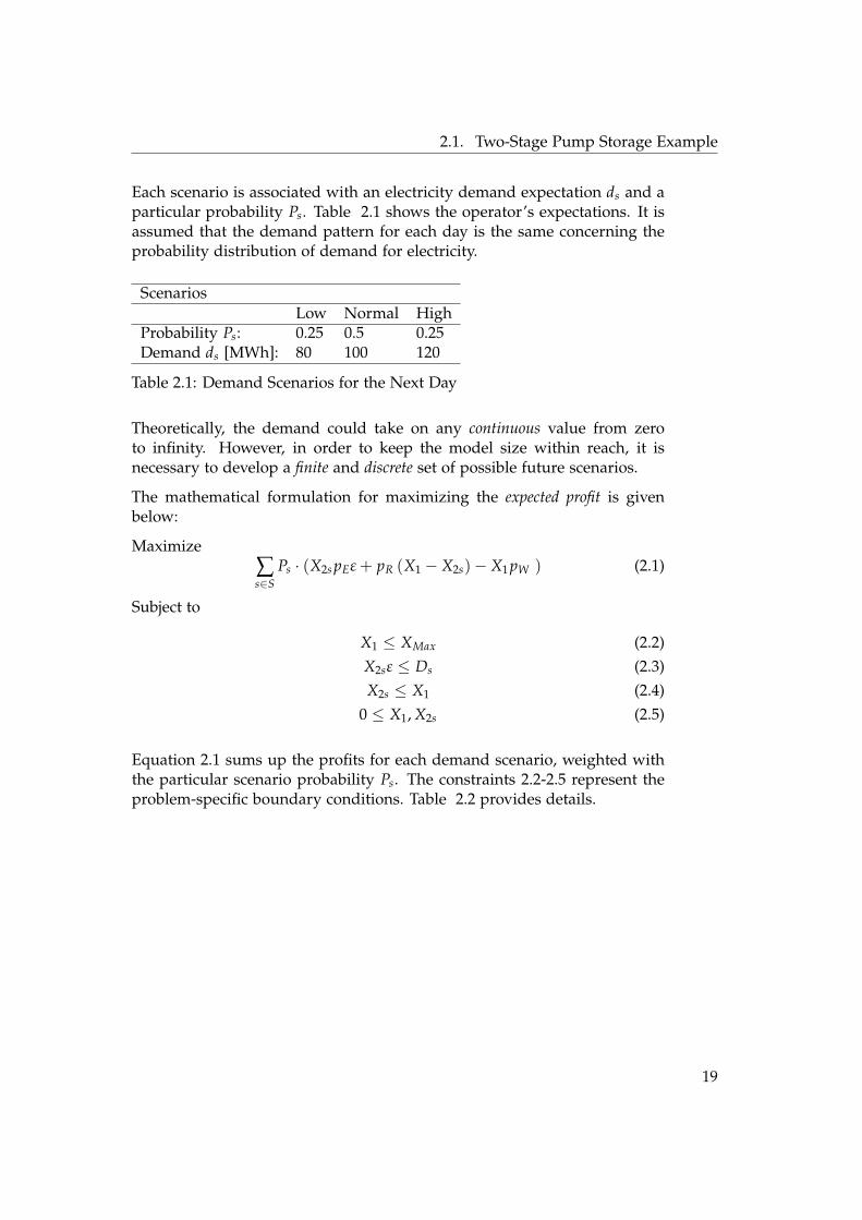
Each scenario is associated with an electricity demand expectation ds and aparticular probability Ps. Table 2.1 shows the operator’s expectations. It isassumed that the demand pattern for each day is the same concerning theprobability distribution of demand for electricity.
ScenariosLow Normal High
Probability Ps: 0.25 0.5 0.25Demand ds [MWh]: 80 100 120
Table 2.1: Demand Scenarios for the Next Day
Theoretically, the demand could take on any continuous value from zeroto infinity. However, in order to keep the model size within reach, it isnecessary to develop a finite and discrete set of possible future scenarios.
The mathematical formulation for maximizing the expected profit is givenbelow:
Maximize∑s∈S
Ps · (X2s pEε + pR (X1 − X2s)− X1 pW ) (2.1)
Subject to
X1 ≤ XMax (2.2)X2sε ≤ Ds (2.3)X2s ≤ X1 (2.4)
0 ≤ X1, X2s (2.5)
Equation 2.1 sums up the profits for each demand scenario, weighted withthe particular scenario probability Ps. The constraints 2.2-2.5 represent theproblem-specific boundary conditions. Table 2.2 provides details.
19

2. Stochastic Programming
Notation: Description: Value:X1 : How much water to pump during night-
time.X2s : How much water to release under sce-
nario s ∈ S ={low, medium, high}XMax : Maximum amount that can be pumped
up during the night.60,000 m3
ε: Amount of energy that can be producedper amount of water.
2.5 KWh/m3
pW : Pumping price 0.075 CHF/m3
pE : Electricity price 0.1 CHF/KWhpR : Water reselling price 0.01 CHF/m3
Table 2.2: Constraints
As shown in the GAMS solution output, the optimal first-stage decisionmaximizing expected profits would be to pump up 40,000 m3 of water eachnight. The recourse decision depends on the scenarios.
In case of low demand, the operator will produce 32, 000 m3 · 2.5 KWh/m3 =80, 000 KWh, the remaining 8000 m3 will be sold back to the local brewerycompany. In the case of normal or high demand, the operator will produce40, 000 m3 · 2.5 KWh/m3 = 100, 000 KWh.
The overall expected profit amounts to 6520 CHF.
*-------------------------------------------------------------------------------
---- VAR X1
X1 First stage decision: How much water to pump
LOWER LEVEL UPPER MARGINAL
. 40000.000 60000.000 .
---- VAR X2
X2 Second stage decision: How much water to release
LOWER LEVEL UPPER MARGINAL
low . 32000.000 +INF .
medium . 40000.000 +INF .
high . 40000.000 +INF .
...
---- VAR Exp_Profit
Exp_Profit Expected Profit of the whole day
LOWER LEVEL UPPER MARGINAL
-INF 6520.000 +INF .
*-------------------------------------------------------------------------------
20
2.1. Two-Stage Pump Storage Example
Of course, the recourse decision in the above example is trivial. The fixedelectricity price means that the operator will release as much water as pos-sible with respect to the electricity demand. The operator will be alwaysbetter off producing electricity than by reselling the water back to the localbeverage company.
However, the recourse decision would become more complex in a modelin which not only the demand but also the electricity price or the resellingprice of the water were described with stochastic coefficients.
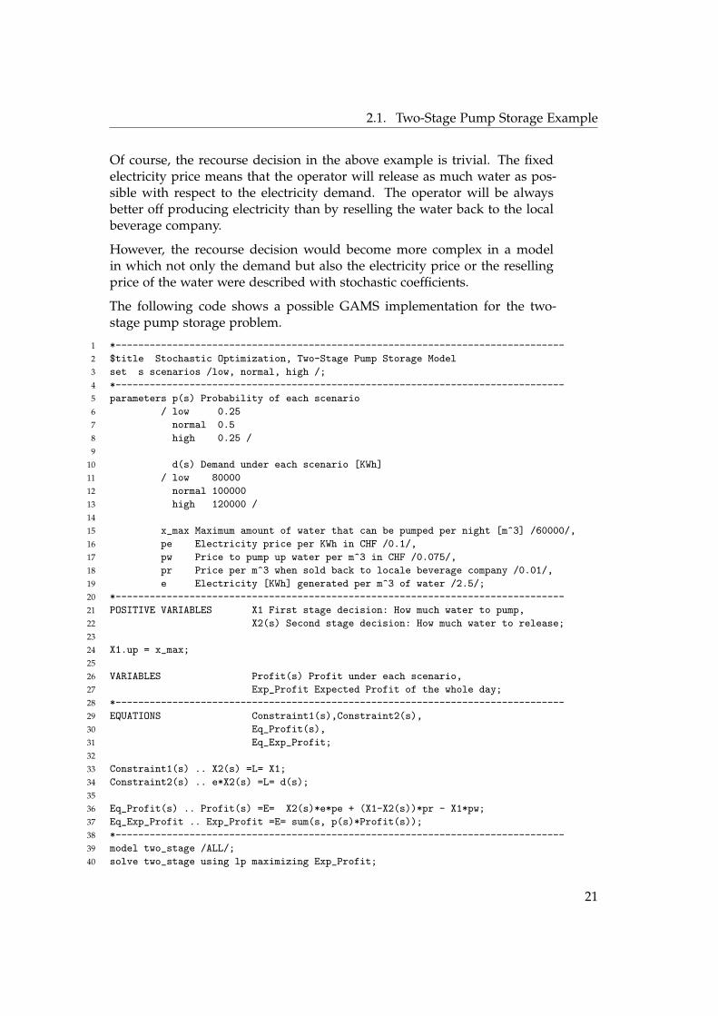
The following code shows a possible GAMS implementation for the two-stage pump storage problem.
1 *-------------------------------------------------------------------------------
2 $title Stochastic Optimization, Two-Stage Pump Storage Model
3 set s scenarios /low, normal, high /;
4 *-------------------------------------------------------------------------------
5 parameters p(s) Probability of each scenario
6 / low 0.25
7 normal 0.5
8 high 0.25 /
9
10 d(s) Demand under each scenario [KWh]
11 / low 80000
12 normal 100000
13 high 120000 /
14
15 x_max Maximum amount of water that can be pumped per night [m^3] /60000/,
16 pe Electricity price per KWh in CHF /0.1/,
17 pw Price to pump up water per m^3 in CHF /0.075/,
18 pr Price per m^3 when sold back to locale beverage company /0.01/,
19 e Electricity [KWh] generated per m^3 of water /2.5/;
20 *-------------------------------------------------------------------------------
21 POSITIVE VARIABLES X1 First stage decision: How much water to pump,
22 X2(s) Second stage decision: How much water to release;
23
24 X1.up = x_max;
25
26 VARIABLES Profit(s) Profit under each scenario,
27 Exp_Profit Expected Profit of the whole day;
28 *-------------------------------------------------------------------------------
29 EQUATIONS Constraint1(s),Constraint2(s),
30 Eq_Profit(s),
31 Eq_Exp_Profit;
32
33 Constraint1(s) .. X2(s) =L= X1;
34 Constraint2(s) .. e*X2(s) =L= d(s);
35
36 Eq_Profit(s) .. Profit(s) =E= X2(s)*e*pe + (X1-X2(s))*pr - X1*pw;
37 Eq_Exp_Profit .. Exp_Profit =E= sum(s, p(s)*Profit(s));
38 *-------------------------------------------------------------------------------
39 model two_stage /ALL/;
40 solve two_stage using lp maximizing Exp_Profit;
21

2. Stochastic Programming
2.2 Multi-Stage Problems
In reality, most decision processes are not limited to only two stages. Amulti-period setting requires several decisions to be made throughout apath of uncertain events. Because the events that take place in each timeperiod are unknown by the decision maker, they are described with thehelp of stochastic quantities. Depending on one’s perspective, the decisionsare taken either at the beginning or the end of a specific time period. Ateach decision stage, the best action is sought with respect to observed pastevents and in anticipation of as yet unknown future realizations.
As in the two-stage case, the expectations for the future are captured by afinite and discrete set of possible scenarios S = {s1, s2, ..., sN}. In contrastto the two-stage problem, however, the final scenarios may develop overseveral time periods. Scenario trees are used to illustrate the evolution ofdifferent realizations.
s1 s2 s3 s4
Stage 1:
Stage 2:
Stage 3:
t = 1
t = 2
t = 3
Figure 2.1: Three-stage binary scenario tree.
The construction of a comprehensive and representative scenario set for theinvolved stochastic quantities is a challenging task. Depending on the un-derlying stochastic variable, there are several different approaches that canbe used to generate a meaningful set of scenarios. For example, the inflowscenarios can be based on the previous year’s precipitation data, assumingthat the inflow obeys a seasonal pattern. A more promising approach wouldprobably be to use current meteorological forecasts, or even a combinationof historical inflows and future weather prognoses. The question of how toassign probabilities to each scenario must also be considered. A thorough
22

2.2. Multi-Stage Problems
discussion on scenario generation is beyond the scope of this text: pleaserefer to [7] for a brief introduction to the subject.
23

2. Stochastic Programming
2.3 Clear Lake Dam Example
The following stochastic multi-stage optimization model was designed inthe style of the Clear Lake Dam textbook example described in [1]. A solutionto the original problem can be found in the GAMS model library.
A reservoir operator faces the following costs:
• Shortfall costs CS for each mm below a minimum reservoir height LMin
• Flooding costs CF for each mm above a maximum reservoir height LMax
Based on the inflow expectations for the next three months (January, Februaryand March), the operator sets up a stochastic multi-stage model to determinethe optimal recourse decisions that minimize the expected costs of all deci-sions made. As soon as the realization of the stochastic inflow has beenobserved for a given month, the operator makes a release decision that re-sponds to this particular realization in consideration of its impact on laterstages.
It is assumed that there are three possible inflow realizations for each monthlow, normal, and high each of which has its own particular probability. Theoperator’s expectations are given below:
Realizations: Low Normal HighProbability PR: 0.25 0.5 0.25Inflow IR [m]: 50 150 350
Table 2.3: Inflow scenarios
24

2.3. Clear Lake Dam Example
Note that the inflow expectations are the same for each month, independentof one another. Table 2.4 describes the physical constraints of the Clear LakeDam.
Notation: Description: Value:RMax : Maximum amount of water that can be
released per month200 [mm]
LMax : Maximum reservoir height 250 [mm]LStart : Reservoir height at the beginning of the
planning horizon (end of December)100 [mm]
cS : Shortfall costs CS for each mm below min-imum reservoir height LMin = 0
5000 CHF/mm
cS : Flooding costs CF for each mm abovemaximum reservoir height LMax
10,000CHF/mm
Table 2.4: Constraints: Note that the unit describing the fill quantity standsfor [mm] reservoir height.
From a mathematical standpoint, the stochastic optimization problem canbe formulated and solved as a deterministic linear program (LP) similar tothe example in the first chapter. However, with regard to the implementa-tion with GAMS, a range of approaches are used to model the optimizationproblem. Here, a distinction is made between node-based and scenario-basedscenario tree descriptions.
25
2. Stochastic Programming
2.3.1 Node-Based Notation
n3n1
n4
n2
n5n14n15n16n17n18n19n20n21n22n23n24n25n26n27n28n29n30n31n32n33n34n35n36n37n38n39n40
n6
n7
n8
n9
n10
n11
n12
n13s27s26s25...
s3s2s1
s27s26s25
...
t: dec jan feb mar
2. 3. 4.1.Stages:
Realizations:1: low
2: normal
3: high
Figure 2.2: Node-Based Tree
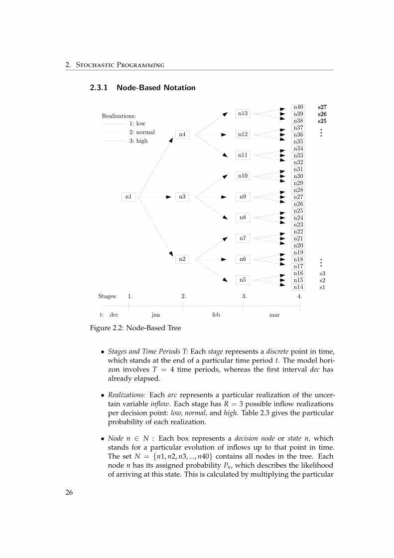
• Stages and Time Periods T: Each stage represents a discrete point in time,which stands at the end of a particular time period t. The model hori-zon involves T = 4 time periods, whereas the first interval dec hasalready elapsed.
• Realizations: Each arc represents a particular realization of the uncer-tain variable inflow. Each stage has R = 3 possible inflow realizationsper decision point: low, normal, and high. Table 2.3 gives the particularprobability of each realization.
• Node n ∈ N : Each box represents a decision node or state n, whichstands for a particular evolution of inflows up to that point in time.The set N = {n1, n2, n3, ..., n40} contains all nodes in the tree. Eachnode n has its assigned probability Pn, which describes the likelihoodof arriving at this state. This is calculated by multiplying the particular
26
2.3. Clear Lake Dam Example
probabilities PR of the previous realizations that have resulted in staten. Pn10, for example, is given by Pnormal · Phigh = 0.5 · 0.25 = 0.125, whilePn33 is given by Phigh · Plow · Pnormal = 0.25 · 0.25 · 0.5 = 0.03125. Thereare 40 nodes in our scenario tree.1
• Scenarios s ∈ S: A scenario s represents a particular path from the rootnode n1 to a lea f node at the end of the last time period. The numberof scenarios is given by RT−1 = 33 = 27. The set S = {s1, s2, ..., s27}contains all scenarios.
• Parent Nodes: For each node n (except for the first node), the functionparent(n) points to its particular predecessor node. parent(n17), forexample, is equal to n6. The mapping between parent and child nodesis required to formulate the reservoir balance for all states n.
The above notation makes it possible to mathematically formulate the ClearLake optimization problem as follows:
Minimize∑
n∈NPn(csZn + c f Fn) , (2.7)
Subject to
Ln = Lparent(n) + In + Zn − Rn − Fn ∀n ∈ N \ n = n1, (2.8)
0 ≤ Rn ≤ Rmax ∀n ∈ N, (2.9)0 ≤ Ln ≤ Lmax ∀n ∈ N, (2.10)
0 ≤ Zn, Fn ∀n ∈ N, (2.11)Ln1 = Lstart (2.12)
Where Zn denotes the amount of water imported at node n, Fn denotes theamount of floodwater released at node n, and Rn denotes the amount ofwater released normally at node n. The unit of all these variables is ’[mm]reservoir height’. Equation 2.8 describes the physical reservoir balance foreach state n.
The water height at stage n is given by the water height at the predecessorstate Lparent(n) plus the water inflows In and the water import, Zn, minus thewater released normally, Rn, and the floodwater released, Fn.
The next page shows an implementation with GAMS of the described prob-lem:
1 The total number of nodes TN in a symmetric scenario tree is given by:
TN =T−1
∑i=0
Ri, (2.6)
where R = number of realizations and T = number of time periods.
27
2. Stochastic Programming
1 *-------------------------------------------------------------------------------
2 $title Stochastic, Multi-Stage Reservoir Release model, Node-Based Notation
3 $ontext
4 Designed in the style of the Clear Lake Dam example found in the GAMS model
5 library
6 $offtext
7 *-------------------------------------------------------------------------------
8 *Sets are defined
9
10 sets r Stochastic realizations (precipitation) /low, normal, high/
11 t Time periods /dec,jan,feb,mar/
12 n Nodes: Decision points or states in scenario tree /n1*n40/,
13 base_t(t) First period /dec/,
14 root(n) The root node: /n1/;
15
16 * The alias command allows to define sets that act in
17 * the same way as an already defined set:
18
19 alias (n,child,parent);
20
21
22 set anc(child,parent) Set which maps each node to predecessor node
23
24 /(n2,n3,n4).n1, (n5,n6,n7).n2, (n8,n9,n10).n3, (n11,n12,n13).n4,
25 (n14,n15,n16).n5, (n17,n18,n19).n6,(n20,n21,n22).n7, (n23,n24,n25).n8,
26 (n26,n27,n28).n9, (n29,n30,n31).n10,(n32,n33,n34).n11,(n35,n36,n37).n12,
27 (n38,n39,n40).n13/;
28
29 * This is an ancillary set that is needed below to formulate the equations:
30
31 set nt(n,t) Association of nodes with time periods
32
33
34 /n1.dec,
35 (n2,n3,n4).jan,
36 (n5,n6,n7,n8,n9,n10,n11,n12,n13).feb,
37 (n14,n15,n16,n17,n18,n19,n20,n21,n22,n23,n24,n25,n26,n27,n28,n29,n30,
38 n31,n32,n33,n34,n35,n36,n37,n38,n39,n40).mar/;
39
40 * This is an ancillary set that is needed below to assign the node
41 * specific inflows and probabilities:
42
43 set nr(n,r) Association of nodes and realizations
44
45 /(n2,n5,n8,n11,n14,n17,n20,n23,n26,n29,n32,n35,n38).low,
46 (n3,n6,n9,n12,n15,n18,n21,n24,n27,n30,n33,n36,n39).normal,
47 (n4,n7,n10,n13,n16,n19,n22,n25,n28,n31,n34,n37,n40).high/;
48 *-------------------------------------------------------------------------------
49 *Parameters are specified
50
51 parameter pr(r) Probability distribution over realizations
52 /low 0.25,
53 normal 0.50
54 high 0.25 /,
28

2.3. Clear Lake Dam Example
55
56 inflow(r) Inflow under realization r
57 /low 50,
58 normal 150,
59 high 350 /,
60
61 floodcost ’Flooding penalty cost thousand CHF/mm’ /10/,
62 lowcost ’Water importation cost thousand CHF/mm’ /5/,
63 l_start ’Initial water level (mm)’ /100/,
64 l_max ’Maximum reservoir level (mm)’ /250/,
65 r_max ’Maximum normal release in any period’ /200/;
66
67 * Here we assign the node specific inflows:
68
69 parameter n_inflow(n) Water inflow at each node;
70 n_inflow(n)$[not root(n)] = sum{(nr(n,r)),inflow(r)};
71
72 * The probability to arrive at a specific node is calculated for
73 * each node, syntax is explained in Chapter three:
74
75 parameter n_prob(n) Probability of being at any node;
76 n_prob(root) = 1;
77 loop {anc(child,parent),
78 n_prob(child) = sum {nr(child,r), pr(r)}*n_prob(parent);};
79 *-------------------------------------------------------------------------------
80 * Model logic:
81
82 variable EC ’Expected costs’;
83
84 positive variable L(n,t) ’Reservoir water level -- EOP’
85 Release(n,t) ’Normal release of water (mm)’
86 F(n,t) ’Floodwater released (mm)’
87 Z(n,t) ’Water imports (mm)’;
88
89 equations ecdef, ldef;
90
91 ecdef..
92 EC =e= sum {nt(n,t),n_prob(n)*[floodcost*F(n,t)+lowcost*Z(n,t)]};
93
94 ldef(nt(n,t))$[not root(n)]..
95 L(n,t) =e= sum{anc(n,parent),l(parent,t-1)}+n_inflow(n)+Z(n,t)-Release(n,t)-F(n,t);
96
97 Release.up(n,t) = r_max;
98 L.up(n,t) = l_max;
99 L.fx(n,base_t) = l_start;
100 *-------------------------------------------------------------------------------
101 model mincost / ecdef, ldef /;
102 solve mincost using LP minimizing EC;
103 *-------------------------------------------------------------------------------
29
2. Stochastic Programming
2.3.2 Scenario-Based Notation
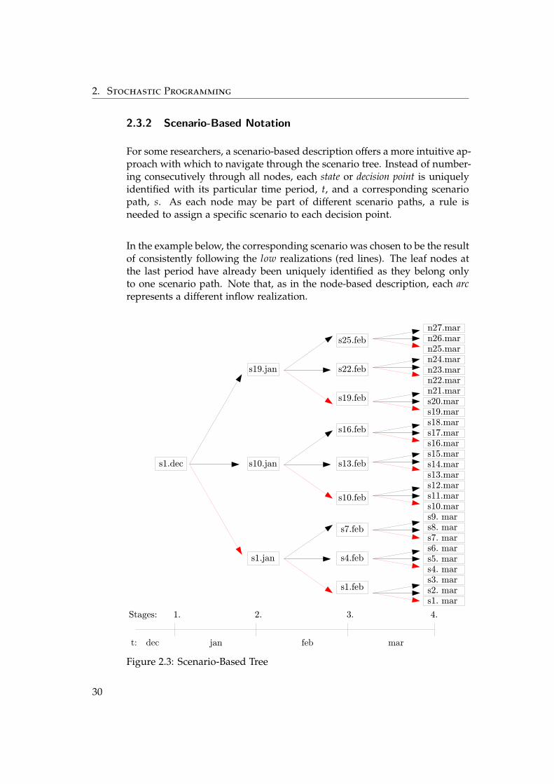
For some researchers, a scenario-based description offers a more intuitive ap-proach with which to navigate through the scenario tree. Instead of number-ing consecutively through all nodes, each state or decision point is uniquelyidentified with its particular time period, t, and a corresponding scenariopath, s. As each node may be part of different scenario paths, a rule isneeded to assign a specific scenario to each decision point.
In the example below, the corresponding scenario was chosen to be the resultof consistently following the low realizations (red lines). The leaf nodes atthe last period have already been uniquely identified as they belong onlyto one scenario path. Note that, as in the node-based description, each arcrepresents a different inflow realization.
t: dec jan feb mar
2. 3. 4.1.Stages:
s1.dec s10.jan
s1.jan
s19.jan s22.feb
s25.feb
s19.feb
s13.feb
s16.feb
s10.feb
s4.feb
s7.feb
s1.feb
s1. mars2. mars3. mars4. mars5. mars6. mars7. mars8. mars9. mars10.mars11.mars12.mars13.mars14.mars15.mars16.mars17.mars18.mars19.mars20.marn21.marn22.marn23.marn24.marn25.marn26.marn27.mar
Figure 2.3: Scenario-Based Tree
30

2.3. Clear Lake Dam Example
Apart from notational differences, the mathematical model stays the same,regardless of whether a scenario-based description or a node-based tree de-scription is used. However, in terms of the GAMS implementation, a differ-ent concept is used in order to keep track of the relationships between thedecision points.
• Equilibrium Set eq(s,t): As described above, each decision point or statein the tree is uniquely identified with its time period and a particularscenario path. The set eq(s, t) = {s1.dec, s1.jan, ..., s27.mar} contains allcombinations of the sets time and scenario, which, together, identify aparticular decision point.
• Offset Pointer o(s,t): The offset pointer is the equivalent to the parentfunction parent(n) in the node-based case. It is used to map eachdecision point to its predecessor in order to formulate the reservoirbalance equation. Due to the specific assignment rule that was used todefine the equilibrium set eq(s,t), two adjacent equilibrium points maybe labeled by different scenarios even though they are both part of thesame scenario path. Therefore, a method is needed to keep track ofthe relation between the scenario of a specific equilibrium point eq(s,t)and the scenario of its predecessor point.
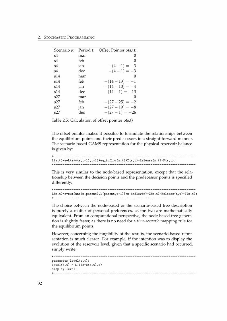
The calculation of the offset pointer o(s,t) is based on an ordered scenarioset. Each of the 27 scenarios in the example has a specific position number,as Table 2.4 shows. The offset pointer o(s,t) is given by the number thatrepresents the offset of scenario s in time period t. By definition, the offsetpointers for equilibrium points at the last stage are always equal to zero.Table 2.5 (together with Figure 2.3) illustrates the calculation of the offsetpointer.
s10 s11 s12s7 s8 s9s4 s5 s6s1 s2 s3 s19s16 s17 s18s13 s14 s15Element:
Position Nr: 1 2 3 4 5 6 7 8 9 10 11 12 13 14 15 16 17 18 19
......
Figure 2.4: Ordered Set
31
2. Stochastic Programming
Scenario s: Period t: Offset Pointer o(s,t):s4 mar 0s4 feb 0s4 jan −(4− 1) = −3s4 dec −(4− 1) = −3s14 mar 0s14 feb −(14− 13) = −1s14 jan −(14− 10) = −4s14 dec −(14− 1) = −13s27 mar 0s27 feb −(27− 25) = −2s27 jan −(27− 19) = −8s27 dec −(27− 1) = −26
Table 2.5: Calculation of offset pointer o(s,t)
The offset pointer makes it possible to formulate the relationships betweenthe equilibrium points and their predecessors in a straight-forward manner.The scenario-based GAMS representation for the physical reservoir balanceis given by:
*-------------------------------------------------------------------------------
L(s,t)=e=L(s+o(s,t-1),t-1)+eq_inflow(s,t)+Z(s,t)-Release(s,t)-F(s,t);
*-------------------------------------------------------------------------------
This is very similar to the node-based representation, except that the rela-tionship between the decision points and the predecessor points is specifieddifferently:
*-------------------------------------------------------------------------------
L(n,t)=e=sum{anc(n,parent),l(parent,t-1)}+n_inflow(n)+Z(n,t)-Release(n,t)-F(n,t);
*-------------------------------------------------------------------------------
The choice between the node-based or the scenario-based tree descriptionis purely a matter of personal preferences, as the two are mathematicallyequivalent. From an computational perspective, the node-based tree genera-tion is slightly faster, as there is no need for a time-scenario mapping rule forthe equilibrium points.
However, concerning the tangibility of the results, the scenario-based repre-sentation is much clearer. For example, if the intention was to display theevolution of the reservoir level, given that a specific scenario had occurred,simply write:
*-------------------------------------------------------------------------------
parameter level(s,t);
level(s,t) = L.l(s+o(s,t),t);
display level;
*-------------------------------------------------------------------------------
32
2.3. Clear Lake Dam Example
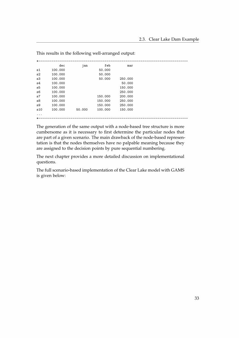
This results in the following well-arranged output:
*-------------------------------------------------------------------------------
dec jan feb mar
s1 100.000 50.000
s2 100.000 50.000
s3 100.000 50.000 250.000
s4 100.000 50.000
s5 100.000 150.000
s6 100.000 250.000
s7 100.000 150.000 200.000
s8 100.000 150.000 250.000
s9 100.000 150.000 250.000
s10 100.000 50.000 100.000 150.000
...
*-------------------------------------------------------------------------------
The generation of the same output with a node-based tree structure is morecumbersome as it is necessary to first determine the particular nodes thatare part of a given scenario. The main drawback of the node-based represen-tation is that the nodes themselves have no palpable meaning because theyare assigned to the decision points by pure sequential numbering.
The next chapter provides a more detailed discussion on implementationalquestions.
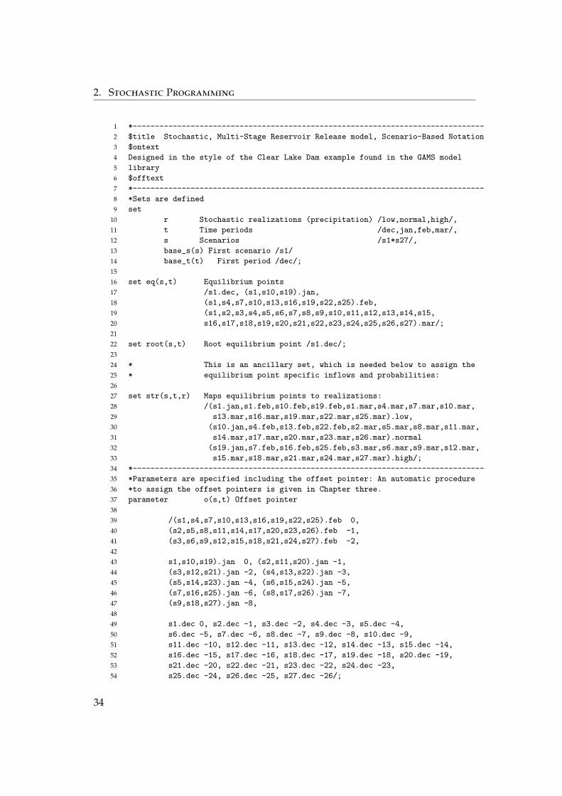
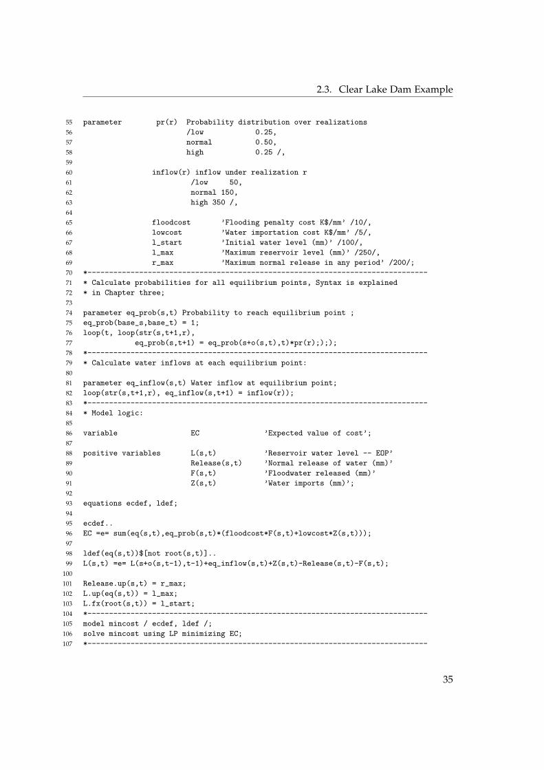
The full scenario-based implementation of the Clear Lake model with GAMSis given below:
33
2. Stochastic Programming
1 *-------------------------------------------------------------------------------
2 $title Stochastic, Multi-Stage Reservoir Release model, Scenario-Based Notation
3 $ontext
4 Designed in the style of the Clear Lake Dam example found in the GAMS model
5 library
6 $offtext
7 *-------------------------------------------------------------------------------
8 *Sets are defined
9 set
10 r Stochastic realizations (precipitation) /low,normal,high/,
11 t Time periods /dec,jan,feb,mar/,
12 s Scenarios /s1*s27/,
13 base_s(s) First scenario /s1/
14 base_t(t) First period /dec/;
15
16 set eq(s,t) Equilibrium points
17 /s1.dec, (s1,s10,s19).jan,
18 (s1,s4,s7,s10,s13,s16,s19,s22,s25).feb,
19 (s1,s2,s3,s4,s5,s6,s7,s8,s9,s10,s11,s12,s13,s14,s15,
20 s16,s17,s18,s19,s20,s21,s22,s23,s24,s25,s26,s27).mar/;
21
22 set root(s,t) Root equilibrium point /s1.dec/;
23
24 * This is an ancillary set, which is needed below to assign the
25 * equilibrium point specific inflows and probabilities:
26
27 set str(s,t,r) Maps equilibrium points to realizations:
28 /(s1.jan,s1.feb,s10.feb,s19.feb,s1.mar,s4.mar,s7.mar,s10.mar,
29 s13.mar,s16.mar,s19.mar,s22.mar,s25.mar).low,
30 (s10.jan,s4.feb,s13.feb,s22.feb,s2.mar,s5.mar,s8.mar,s11.mar,
31 s14.mar,s17.mar,s20.mar,s23.mar,s26.mar).normal
32 (s19.jan,s7.feb,s16.feb,s25.feb,s3.mar,s6.mar,s9.mar,s12.mar,
33 s15.mar,s18.mar,s21.mar,s24.mar,s27.mar).high/;
34 *-------------------------------------------------------------------------------
35 *Parameters are specified including the offset pointer: An automatic procedure
36 *to assign the offset pointers is given in Chapter three.
37 parameter o(s,t) Offset pointer
38
39 /(s1,s4,s7,s10,s13,s16,s19,s22,s25).feb 0,
40 (s2,s5,s8,s11,s14,s17,s20,s23,s26).feb -1,
41 (s3,s6,s9,s12,s15,s18,s21,s24,s27).feb -2,
42
43 s1,s10,s19).jan 0, (s2,s11,s20).jan -1,
44 (s3,s12,s21).jan -2, (s4,s13,s22).jan -3,
45 (s5,s14,s23).jan -4, (s6,s15,s24).jan -5,
46 (s7,s16,s25).jan -6, (s8,s17,s26).jan -7,
47 (s9,s18,s27).jan -8,
48
49 s1.dec 0, s2.dec -1, s3.dec -2, s4.dec -3, s5.dec -4,
50 s6.dec -5, s7.dec -6, s8.dec -7, s9.dec -8, s10.dec -9,
51 s11.dec -10, s12.dec -11, s13.dec -12, s14.dec -13, s15.dec -14,
52 s16.dec -15, s17.dec -16, s18.dec -17, s19.dec -18, s20.dec -19,
53 s21.dec -20, s22.dec -21, s23.dec -22, s24.dec -23,
54 s25.dec -24, s26.dec -25, s27.dec -26/;
34
2.3. Clear Lake Dam Example
55 parameter pr(r) Probability distribution over realizations
56 /low 0.25,
57 normal 0.50,
58 high 0.25 /,
59
60 inflow(r) inflow under realization r
61 /low 50,
62 normal 150,
63 high 350 /,
64
65 floodcost ’Flooding penalty cost K$/mm’ /10/,
66 lowcost ’Water importation cost K$/mm’ /5/,
67 l_start ’Initial water level (mm)’ /100/,
68 l_max ’Maximum reservoir level (mm)’ /250/,
69 r_max ’Maximum normal release in any period’ /200/;
70 *-------------------------------------------------------------------------------
71 * Calculate probabilities for all equilibrium points, Syntax is explained
72 * in Chapter three;
73
74 parameter eq_prob(s,t) Probability to reach equilibrium point ;
75 eq_prob(base_s,base_t) = 1;
76 loop(t, loop(str(s,t+1,r),
77 eq_prob(s,t+1) = eq_prob(s+o(s,t),t)*pr(r);););
78 *-------------------------------------------------------------------------------
79 * Calculate water inflows at each equilibrium point:
80
81 parameter eq_inflow(s,t) Water inflow at equilibrium point;
82 loop(str(s,t+1,r), eq_inflow(s,t+1) = inflow(r));
83 *-------------------------------------------------------------------------------
84 * Model logic:
85
86 variable EC ’Expected value of cost’;
87
88 positive variables L(s,t) ’Reservoir water level -- EOP’
89 Release(s,t) ’Normal release of water (mm)’
90 F(s,t) ’Floodwater released (mm)’
91 Z(s,t) ’Water imports (mm)’;
92
93 equations ecdef, ldef;
94
95 ecdef..
96 EC =e= sum(eq(s,t),eq_prob(s,t)*(floodcost*F(s,t)+lowcost*Z(s,t)));
97
98 ldef(eq(s,t))$[not root(s,t)]..
99 L(s,t) =e= L(s+o(s,t-1),t-1)+eq_inflow(s,t)+Z(s,t)-Release(s,t)-F(s,t);
100
101 Release.up(s,t) = r_max;
102 L.up(eq(s,t)) = l_max;
103 L.fx(root(s,t)) = l_start;
104 *-------------------------------------------------------------------------------
105 model mincost / ecdef, ldef /;
106 solve mincost using LP minimizing EC;
107 *-------------------------------------------------------------------------------
35


Chapter 3
Implementation
When dealing with multi-stage stochastic models, a crucial issue is the expo-nential growth of the scenario tree for each additional time period, t, whichis added to the model horizon. This again results in the exponentially grow-ing computation time it takes GAMS to solve the model. As shown in thesolution report below, the Clear Lake model from the previous chapter (in-cluding 27 scenarios) was solved in roughly te= 0.1 seconds.
*-------------------------------------------------------------------------------
--- Starting compilation
--- multi.gms(105) 3 Mb
--- Starting execution: elapsed 0:00:00.004
--- ...
--- Executing CPLEX: elapsed 0:00:00.009
--- multi.gms(101) 4 Mb:00:00.086
--- ...
--- Executing after solve: elapsed 0:00:00.113
*** Status: Normal completion
--- Job multi.gms Stop 05/03/11 15:05:40 elapsed 0:00:00.114
*-------------------------------------------------------------------------------
However, as shown in Figure 3.1 on the next page, the execution time rapidlyincreases if the model horizon is extended. Figure 3.1 also shows that theexponential growth is intensified if the number of possible stochastic realiza-tions R is increased at each decision node.
This chapter introduces measures to mitigate the exponentially growing ex-ecution time of stochastic multi-stage problems, focusing on the implemen-tation with GAMS.
37

3. Implementation
Figure 3.1: GAMS execution time for the Clear Lake model: T=6 time peri-ods.
Figure 3.2: GAMS execution time for the Clear Lake model: R=6 realizations.
38

3.1. Dynamic Set Assignments
3.1 Dynamic Set Assignments
The Clear Lake Dam model from the previous chapter explicitly named themembers of each set in the source code. However, this can become tediousas the problem size grows, so GAMS allows the automatic creation of setmembers by defining an assignment rule. To allocate set memberships dy-namically, the following syntax can be used:
set_name(domain_name)$[condition] = yes | no
A detailed discussion on dynamic sets is given in [9]. Of course, the partic-ular condition to assign set memberships depends on the model structureand the characteristics of the specific set.
Considering a node-based tree description, conditions must be determinedfor the following three sets: (i) the ancestor set anc(child,parent), which linkseach node with its predecessor node: (ii) the node-time set nt(n,t), whichlinks each node with its particular time period: and (iii) the node-realizationset nr(n,r), which links each node with its particular inflow realization. Themathematical relationships for these sets are discussed below.
Node-Predecessor Mapping: parent(n)
The node number of the predecessor of node n is given by the followingfunction:
parent(n) =⌊(n + R− 2)
R
⌋(3.1)
Where n is the node number as defined in Figure 2.2 and R is the totalnumber of stochastic realizations per decision point. Note that the first noden1 has no predecessor node.
Example:
As shown in Figure 2.2 (R = 3), the predecessor of node n12 is n4, which isgiven by:
parent(12) =⌊(12 + 3− 2)
3
⌋= 4 (3.2)
Note that the brackets bxc map the argument x to the largest previous inte-ger, for example, b3.56c = 3.
39

3. Implementation
Node-Realization Mapping: r(n)
The realization r, which corresponds to node n, is given by:
r(n) = (n + R− 2) (mod R) + 1 (3.3)
Note that the first node, n1, has no assigned realization r.
Example:
Assuming that there are R = 3 realizations per decision point (low (1), normal(2) and high (3)), as described in Figure 2.2, the realization r, which hasresulted in node n26, is low (1) given by:
r(26) = (26 + 3− 2) (mod 3) + 1 = 1 (3.4)
Node-Time Mapping: t(n)
The time period, t, which corresponds to node n, is given by the followingalgorithm:
For each time period t:
Check for node n whether condition 3.5 is true:
Rt−1
R− 1≤ n <
Rt
R− 1; (3.5)
If the condition is true,
Return t as the corresponding time period for n
Example:
Assuming that there are R = 3 realizations per decision point and T = 4time periods (dec (1), jan (2), feb (3) and mar(4)), as described in Figure 2.2,the time period for node n11 is equal to t = f eb (3) as condition 3.5 is truefor t = 3:
33−1
3− 1= 4.5 ≤ 11 <
33
3− 1= 13.5 (3.6)
The described mathematical conditions can now be used to dynamicallyassign set memberships with GAMS as shown in the following code:
40

3.1. Dynamic Set Assignments
*------------------------------------------------------------------------------
alias (n,child,parent);
set anc(child,parent) Association of each node with corresponding parent node;
anc(child,parent)$[floor((ord(child)+card(r)-2)/card(r)) eq ord(parent)] = yes;
*------------------------------------------------------------------------------
set nr(n,r) Association of each node with corresponding realization;
nr(n,r)$[mod(ord(n)+card(r)-2,card(r))+1 eq ord(r)] = yes;
*------------------------------------------------------------------------------
set nt(n,t) Association of each node with corresponding time period;
loop{t,
nt(n,t)$[power(card(r),ord(t)-1)/(card(r)-1) le ord(n)
and ord(n) lt power(card(r),ord(t))/(card(r)-1)] = yes;
};
*------------------------------------------------------------------------------
By comparison, the following GAMS syntax was used to formulate the as-signment rules:
• card(set name): The cardinality operator gives back the number ofelements of a specific set. In the case of the Clear Lake example,card(s) = 27, which means that the scenario set contains 27 elements.
• ord(set name): The ordinality operator returns the specific positionnumber of a set element. It can only be used together with an or-dered, one-dimensional set. Example: The statements below will as-sign the following values to the parameter position: position(’low’) = 1,position(’normal’) = 2 and position(’high’) = 3.
set s scenarios /low, normal, high/;
parameter position(s);
position(s) = ord(s);
• loop: The loop statement is a programming feature that is used to exe-cute code repeatedly for a certain control domain. The basic structureof a GAMS loop is given by:
loop(set_to_vary,
Statement or statements to execute
);
• mod(x,y): Remainder of the division x/y. Example: mod(7, 2) = 1.
• floor(x): Gives back the largest integer which is greater or equal to x.Example: f loor(2.3) = 2
• le: less than or equal to
• lt: strictly less than
• eq: equal to
Appendix A.1 provides a full implementation of the Clear Lake modelwith dynamic set membership assignments.
41
3. Implementation
3.2 GAMS Limitations
From a computational point of view, the dynamic membership assignmentcan become rather slow for large models, especially when the membershipassignment statements are used within loops.
The total execution time te to process a GAMS model is basically divided intotwo parts:
• The model generation time tg, which is primarily given by the time ittakes GAMS to assign set memberships and generate the equations.
• The model solution time ts, which is needed to actually solve the gen-erated equations with an appropriate solver and to find the optimalmodel variables.
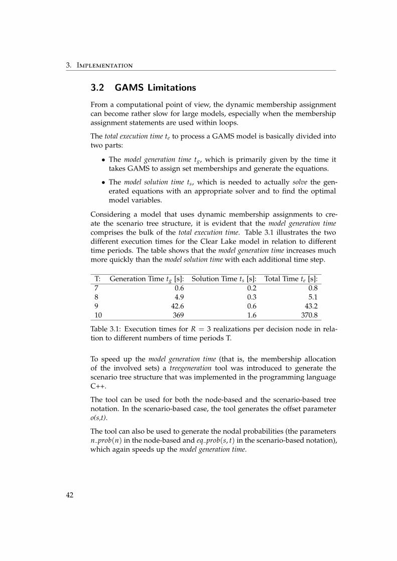
Considering a model that uses dynamic membership assignments to cre-ate the scenario tree structure, it is evident that the model generation timecomprises the bulk of the total execution time. Table 3.1 illustrates the twodifferent execution times for the Clear Lake model in relation to differenttime periods. The table shows that the model generation time increases muchmore quickly than the model solution time with each additional time step.
T: Generation Time tg [s]: Solution Time ts [s]: Total Time te [s]:7 0.6 0.2 0.88 4.9 0.3 5.19 42.6 0.6 43.210 369 1.6 370.8
Table 3.1: Execution times for R = 3 realizations per decision node in rela-tion to different numbers of time periods T.
To speed up the model generation time (that is, the membership allocationof the involved sets) a treegeneration tool was introduced to generate thescenario tree structure that was implemented in the programming languageC++.
The tool can be used for both the node-based and the scenario-based treenotation. In the scenario-based case, the tool generates the offset parametero(s,t).
The tool can also be used to generate the nodal probabilities (the parametersn prob(n) in the node-based and eq prob(s, t) in the scenario-based notation),which again speeds up the model generation time.
42

3.3. Treegeneration tool
3.3 Treegeneration tool
The treegeneration tool is a command line application that communicatesthrough a GDX file with GAMS. A GDX file is a platform independent bi-nary file that can contain information regarding sets, parameters, variables,and equations [6]. GDX files offer a fast and efficient way to pass data fromGAMS to another program or vice versa. The tree generation tool was pro-grammed in C++ and builds upon the API files that can be found in theGAMS home directory.1 The source code of the treegeneration tool is pro-vided in Appendix A.6.
3.3.1 Node-Based Treegeneration
The communication with the tree generation tool involves three steps. Firstly,the user has to save the two sets containing the time periods and the realiza-tions (in the above example t and r) into a GDX file. To save these sets intoa GDX file named cl in.gdx2, we can use the following statement:
*-------------------------------------------------------------------------------
$gdxout cl_in.gdx
$unload t=time_set r=realization_set pr=prob
$gdxout
*-------------------------------------------------------------------------------
The second step is to call the treegeneration tool to create the sets. This isdone with the GAMS statement $call, which allows the command line to beaccessed through GAMS. The correct syntax to start the tree generation is:
*-------------------------------------------------------------------------------
$call treegen.exe cl_in.gdx cl_out.gdx "%gams.sysdir%\"
*-------------------------------------------------------------------------------
The first parameter specifies the input file that contains the time set, therealization set, and the probabilities (cl in.gdx in our example). The secondparameter denotes the output file in which the treegeneration tool will savethe tree structure. The last parameter is used to pass the path of the GAMSdirectory to the program.
The third step is to advise GAMS to import the generated sets from the GDXoutput file cl out.gdx. This can be done using the following syntax:
1API stands for stands for Application Programming Interface. An API code is a softwareinterface between different programs that allows them to communicate with each other. APIexamples for GAMS can be found in the directory /API files in the GAMS home directory.
2The file is saved in the GAMS working directory.
43

3. Implementation
*-------------------------------------------------------------------------------
$gdxin cl_out.gdx
set n Nodes set;
$load n=n
set anc(n,n) Predecessor-mapping for node set;
$load anc=anc
set nr(n,r) Node-realization-mapping;
$load nr=nr
set nt(n,t) Node-time-mapping;
$load nt=nt
parameter n_prob(n) Nodal probabilities;
$load n_prob=n_prob
$gdxin
*-------------------------------------------------------------------------------
The definition of the model variables and the equations stays exactly thesame as in the case without the treegeneration tool. A full implementation ofthe node-based Clear Lake model with the treegeneration tool can be foundin Appendix A.3.
3.3.2 Scenario-Based Treegeneration
The treegeneration tool also creates the offset pointers o(s,t) and the sets thatare necessary for a scenario-based tree description. To use the tool for ascenario-based tree, the user simply needs to import the scenario-based setsand probabilities in the third step, as shown below:
*-------------------------------------------------------------------------------
$gdxout cl_in.gdx
$unload t=time_set r=realization_set pr=prob
$gdxout
*-------------------------------------------------------------------------------
$call treegen.exe cl_in.gdx cl_out.gdx "%gams.sysdir%\"
*-------------------------------------------------------------------------------
$gdxin cl_out.gdx
set s Scenarios - Leaves in the event tree;
$load s=s
set eq(s,t) Equilibrium points - Equivalent to nodes;
$load eq=eq
set str(s,t,r) Association of scenarios with realizations;
$load str=str
parameter o(s,t) Offset pointer;
$load o=offset
parameter eq_prob(s,t) Probability to reach equilibrium point eq;
$load eq_prob=eq_prob
$gdxin
*-------------------------------------------------------------------------------
The rest of the GAMS model (that is, the definition of the model variablesand the equations) is exactly the same as in the model without the treegen-
44

3.3. Treegeneration tool
Figure 3.3: GDXviewer.
eration tool. A full implementation of the scenario-based Clear Lake modelwith the treegeneration tool is provided in Appendix A.2.
A handy tool with which to visualize the binary GDX files is the so-calledgdxviewer, which can be started through the command line. The followingcommand can be used to show the output of the treegeneration tool:
C:\models\scenario-based>gdxviewer cl_out.gdx
45
3. Implementation
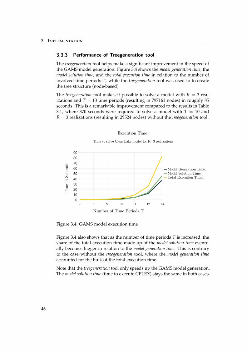
3.3.3 Performance of Treegeneration tool
The treegeneration tool helps make a significant improvement in the speed ofthe GAMS model generation. Figure 3.4 shows the model generation time, themodel solution time, and the total execution time in relation to the number ofinvolved time periods T, while the treegeneration tool was used to to createthe tree structure (node-based).
The treegeneration tool makes it possible to solve a model with R = 3 real-izations and T = 13 time periods (resulting in 797161 nodes) in roughly 85seconds. This is a remarkable improvement compared to the results in Table3.1, where 370 seconds were required to solve a model with T = 10 andR = 3 realizations (resulting in 29524 nodes) without the treegeneration tool.
7 8 9 10 11 12 130102030405060708090
Execution Time
Time to solve Clear Lake model for R=3 realizations
Model Generation Time:Model Solution Time:Total Execution Time:
Number of Time Periods T
Tim
e in
Sec
onds
Figure 3.4: GAMS model execution time
Figure 3.4 also shows that as the number of time periods T is increased, theshare of the total execution time made up of the model solution time eventu-ally becomes bigger in relation to the model generation time. This is contraryto the case without the treegeneration tool, where the model generation timeaccounted for the bulk of the total execution time.
Note that the treegeneration tool only speeds up the GAMS model generation.The model solution time (time to execute CPLEX) stays the same in both cases.
46
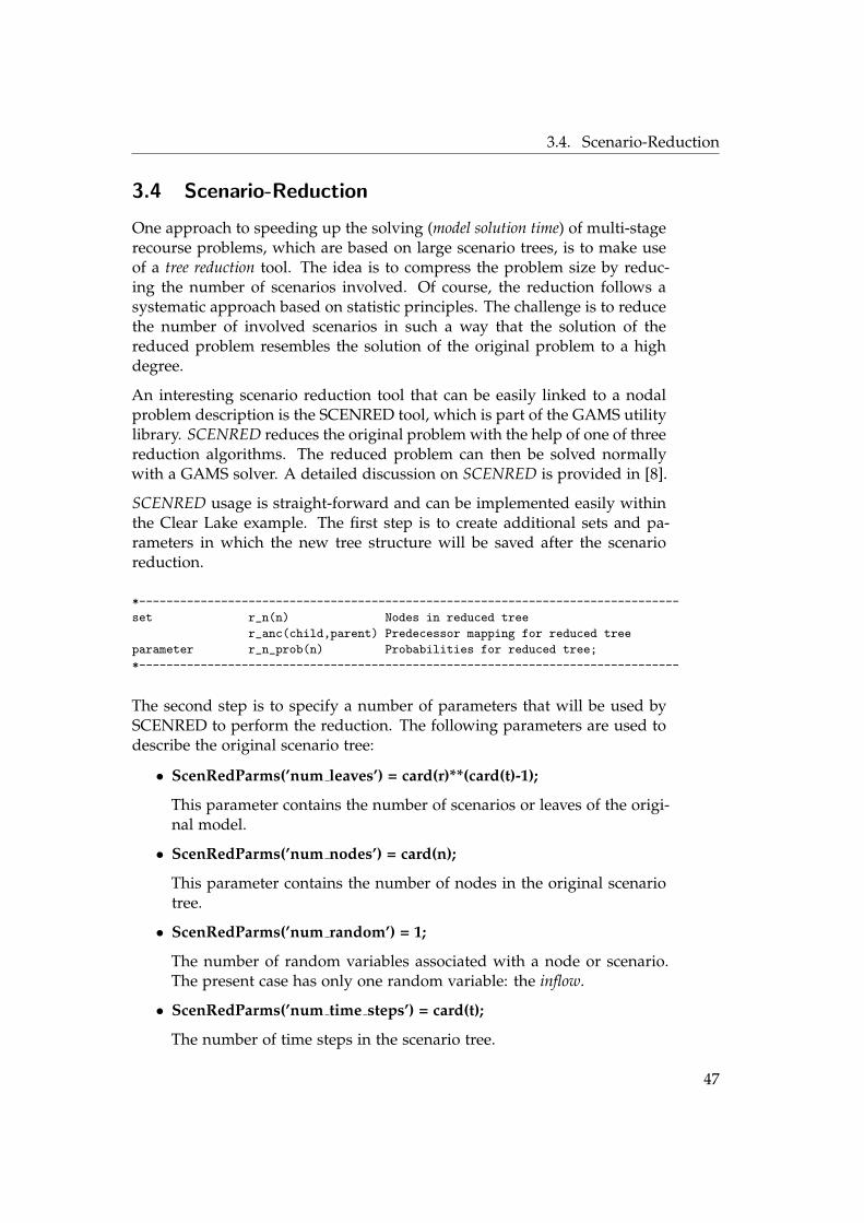
3.4. Scenario-Reduction
3.4 Scenario-Reduction
One approach to speeding up the solving (model solution time) of multi-stagerecourse problems, which are based on large scenario trees, is to make useof a tree reduction tool. The idea is to compress the problem size by reduc-ing the number of scenarios involved. Of course, the reduction follows asystematic approach based on statistic principles. The challenge is to reducethe number of involved scenarios in such a way that the solution of thereduced problem resembles the solution of the original problem to a highdegree.
An interesting scenario reduction tool that can be easily linked to a nodalproblem description is the SCENRED tool, which is part of the GAMS utilitylibrary. SCENRED reduces the original problem with the help of one of threereduction algorithms. The reduced problem can then be solved normallywith a GAMS solver. A detailed discussion on SCENRED is provided in [8].
SCENRED usage is straight-forward and can be implemented easily withinthe Clear Lake example. The first step is to create additional sets and pa-rameters in which the new tree structure will be saved after the scenarioreduction.
*-------------------------------------------------------------------------------
set r_n(n) Nodes in reduced tree
r_anc(child,parent) Predecessor mapping for reduced tree
parameter r_n_prob(n) Probabilities for reduced tree;
*-------------------------------------------------------------------------------
The second step is to specify a number of parameters that will be used bySCENRED to perform the reduction. The following parameters are used todescribe the original scenario tree:
• ScenRedParms(’num leaves’) = card(r)**(card(t)-1);
This parameter contains the number of scenarios or leaves of the origi-nal model.
• ScenRedParms(’num nodes’) = card(n);
This parameter contains the number of nodes in the original scenariotree.
• ScenRedParms(’num random’) = 1;
The number of random variables associated with a node or scenario.The present case has only one random variable: the inflow.
• ScenRedParms(’num time steps’) = card(t);
The number of time steps in the scenario tree.
47

3. Implementation
SCENRED provides the option of choosing between two different criteria tospecify the degree of reduction:
• ScenRedParms(’red percentage’) = 0.5;
This parameter specifies the desired reduction in terms of the relativedistance between the initial and reduced scenario trees (a real numberbetween 0.0 and 1.0)[8]
• ScenRedParms(’red num leaves’) = 15;
This parameter makes it possible to directly specify the number ofleaves in the reduced tree.
Having specified the reduction parameters, these are saved together withthe data that describes the scenario tree in a GDX file. We then advise theSCENRED tool to reduce the tree according to our specifications. The laststep is to read the reduced sets and parameters back into GAMS.
*-------------------------------------------------------------------------------
*Unload the scenario reduction parameters, the node set n, the predecessor
* mapping set anc, the node probabilities n_prob and the inflows at each
* node n_inflow into the GDX file lakein.gdx
execute_unload ’lakein.gdx’, ScenRedParms, n, anc, n_prob, n_inflow;
*-------------------------------------------------------------------------------
*create a text file scenred.opt where we specify the location of the SCENRED
*input file lakein.gdx, the output file lakeout.gdx and the log file lakelog.txt
file opts / ’scenred.opt’ /;
putclose opts ’log_file = lakelog.txt’
/ ’input_gdx lakein.gdx’
/ ’output_gdx = lakeout.gdx’;
*-------------------------------------------------------------------------------
*Run the scenario reduction using the files specified in scenred.opt
execute ’scenred scenred.opt %system.redirlog%’;
*-------------------------------------------------------------------------------
*Read back the reduced scenario tree data from the SCENRED output file
*lakeout.gdx. Save the reduced probabilities in the parameter r_nprob and save
*the parent-child mapping of the reduced tree in the set r_anc.
execute_load ’lakeout.gdx’, ScenRedReport, r_n_prob=red_prob,
r_anc=red_ancestor;
*-------------------------------------------------------------------------------
* To assign the members of the new node set r_n(n) we can simply use the
* following statement
r_n(n)$[r_n_prob(n)]= yes;
*-------------------------------------------------------------------------------
The reduced sets and probabilities can now be used to formulate the equa-tions for the reduced tree. All that is required is to replace the sets that
48
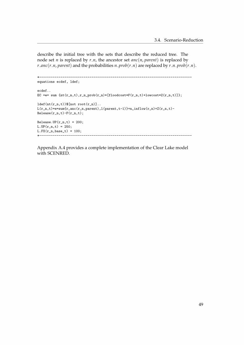
3.4. Scenario-Reduction
describe the initial tree with the sets that describe the reduced tree. Thenode set n is replaced by r n, the ancestor set anc(n, parent) is replaced byr anc(r n, parent) and the probabilities n prob(r n) are replaced by r n prob(r n).
*-------------------------------------------------------------------------------
equations ecdef, ldef;
ecdef..
EC =e= sum {nt(r_n,t),r_n_prob(r_n)*[floodcost*F(r_n,t)+lowcost*Z(r_n,t)]};
ldef(nt(r_n,t))$[not root(r_n)]..
L(r_n,t)=e=sum{r_anc(r_n,parent),l(parent,t-1)}+n_inflow(r_n)+Z(r_n,t)-
Release(r_n,t)-F(r_n,t);
Release.UP(r_n,t) = 200;
L.UP(r_n,t) = 250;
L.FX(r_n,base_t) = 100;
*-------------------------------------------------------------------------------
Appendix A.4 provides a complete implementation of the Clear Lake modelwith SCENRED.
49
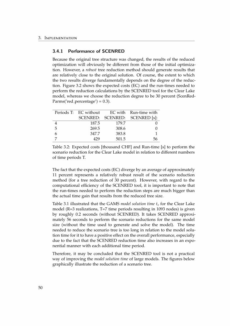
3. Implementation
3.4.1 Performance of SCENRED
Because the original tree structure was changed, the results of the reducedoptimization will obviously be different from those of the initial optimiza-tion. However, a robust tree reduction method should generate results thatare relatively close to the original solution. Of course, the extent to whichthe two results diverge fundamentally depends on the degree of the reduc-tion. Figure 3.2 shows the expected costs (EC) and the run-times needed toperform the reduction calculations by the SCENRED tool for the Clear Lakemodel, whereas we choose the reduction degree to be 30 percent (ScenRed-Parms(’red percentage’) = 0.3).
Periods T: EC without EC with Run-time withSCENRED: SCENRED: SCENRED [s]:
4 187.5 179.7 05 269.5 308.6 06 347.7 383.8 17 429 501.5 56
Table 3.2: Expected costs [thousand CHF] and Run-time [s] to perform thescenario reduction for the Clear Lake model in relation to different numbersof time periods T.
The fact that the expected costs (EC) diverge by an average of approximately11 percent represents a relatively robust result of the scenario reductionmethod (for a tree reduction of 30 percent). However, with regard to thecomputational efficiency of the SCENRED tool, it is important to note thatthe run-times needed to perform the reduction steps are much bigger thanthe actual time gain that results from the reduced tree size.
Table 3.1 illustrated that the GAMS model solution time ts for the Clear Lakemodel (R=3 realizations, T=7 time periods resulting in 1093 nodes) is givenby roughly 0.2 seconds (without SCENRED). It takes SCENRED approxi-mately 56 seconds to perform the scenario reductions for the same modelsize (without the time used to generate and solve the model). The timeneeded to reduce the scenario tree is too long in relation to the model solu-tion time for it to have a positive effect on the overall performance, especiallydue to the fact that the SCENRED reduction time also increases in an expo-nential manner with each additional time period.
Therefore, it may be concluded that the SCENRED tool is not a practicalway of improving the model solution time of large models. The figures belowgraphically illustrate the reduction of a scenario tree.
50

3.5. Computational Framework and Model Specification
Figure 3.5: SCENRED Visualization: Initial Tree
Figure 3.6: SCENRED Visualization: Reduced Tree
3.5 Computational Framework and Model Specification
The treegeneration tool helps to significantly improve the GAMS performanceof our model. However, the inherent problem, which is the exponentialgrowth of the model size with each additional time period, cannot be avoided.
51

3. Implementation
Of course, another way to speed up the solving process is to use a morepowerful computational framework. An interesting possibility would be toimplement the Clear Lake model using the GAMS multi-grid facility. Themain idea of multi-grid computation is to run calculations in parallel on asystem of multiple CPUs. Obviously, the tasks can only be calculated inparallel if their results do not depend on each other. The parallelization ofthe tasks must be coordinated by the programmer in a qualified manner. Anintroduction to GAMS multi-grid computation can be found in [10].
Another way to avoid an uncontrolled growth of the problem size is to clev-erly choose the length of the time periods. Suppose that we wanted to figureout an optimal release schedule for the next week with respect to the inflowprognosis for the whole next year. Instead of choosing a weekly resolutioninvolving 52 time periods, we could define the time periods to have differ-ent lengths. For example, we could say that the first two time periods aresingle weeks, the third period is 10 weeks and the two last periods are each20 weeks. In this case, the model horizon would still be one year, but thenumber of involved time periods could be reduced to five. Choosing timeperiods of different lengths makes sense in most practical settings anyway,as the quality of the inflow prognosis decreases over time. It is obviouslymuch easier to create significant inflow scenarios for the next week than fora particular week in the final quarter of the next year.
52

Chapter 4
Release Model
This chapter illustrates the use of stochastic programming to solve the hydroscheduling problem in a more realistic setting. The following model deter-mines an optimal production schedule for the next day, taking into accountour expectations about future reservoir inflows and electricity prices. It isassumed that the operator plans to sell his production on the day-ahead spotmarket. The basic idea is to find a one-day production plan that balancescurrent profits with expected future profits [3].
By observing the current spot market price for physical delivery on the nextday, the operator must decide how much electricity he is willing to sell, inconsideration of possible future price and inflow developments. The modelaims to evaluate the opportunity to sell electricity at the current spot marketprice against the possibility to sell the production in a future period.
The model includes T = 6 = six time periods (six stages), comprising a totaltime span of roughly one year. The time periods vary in length: the firstperiod t1 is a single day, the second and the third period t2 and t3 are singleweeks, the fourth and fifth periods t4 and t5 are 10 weeks each and the lastperiod t6 is 30 weeks.
t1 t2 t3 t4 t5 t6
Figure 4.1: Scenario-Based Tree
The first-stage decision represents the one-day production plan for the fol-lowing day. The first time period is assumed to be deterministic as the spotmarket prices for delivery on the next day has already been observed. Fur-
53
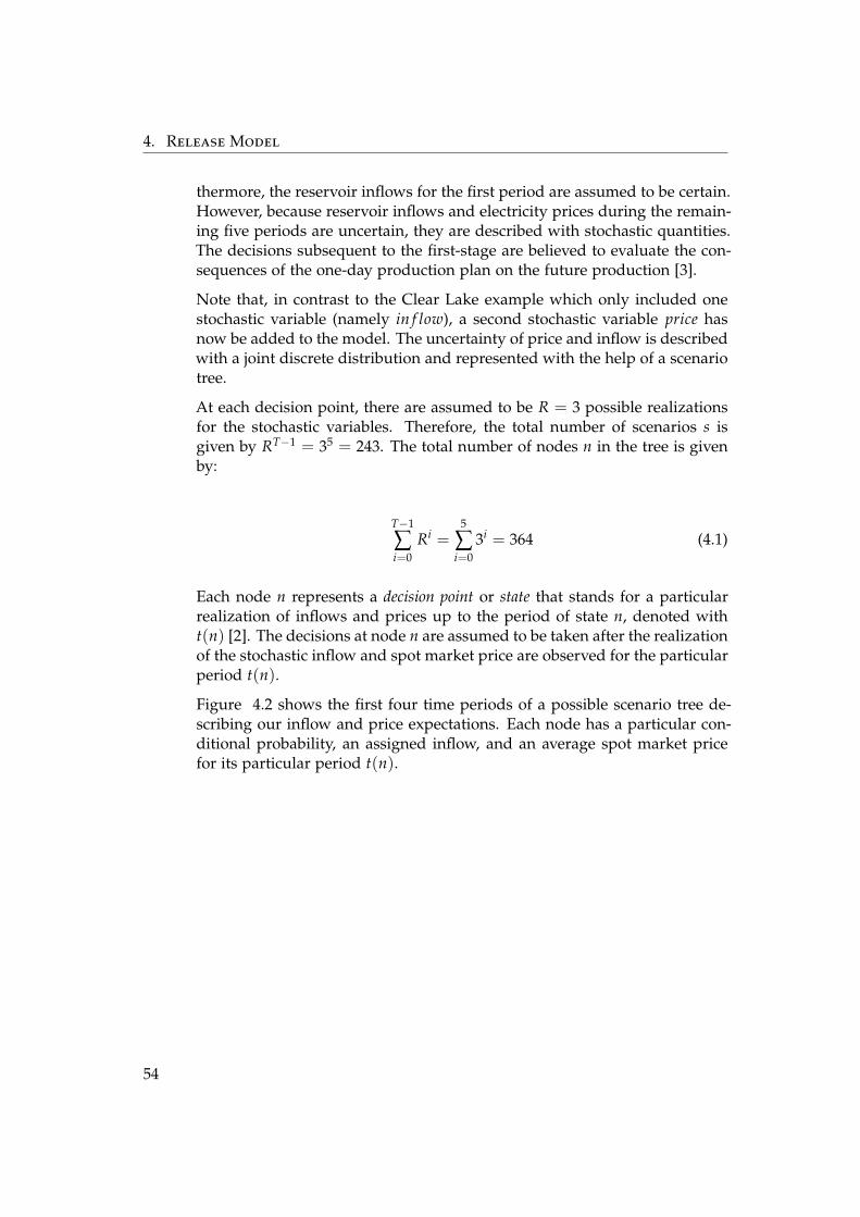
4. Release Model
thermore, the reservoir inflows for the first period are assumed to be certain.However, because reservoir inflows and electricity prices during the remain-ing five periods are uncertain, they are described with stochastic quantities.The decisions subsequent to the first-stage are believed to evaluate the con-sequences of the one-day production plan on the future production [3].
Note that, in contrast to the Clear Lake example which only included onestochastic variable (namely in f low), a second stochastic variable price hasnow be added to the model. The uncertainty of price and inflow is describedwith a joint discrete distribution and represented with the help of a scenariotree.
At each decision point, there are assumed to be R = 3 possible realizationsfor the stochastic variables. Therefore, the total number of scenarios s isgiven by RT−1 = 35 = 243. The total number of nodes n in the tree is givenby:
T−1
∑i=0
Ri =5
∑i=0
3i = 364 (4.1)
Each node n represents a decision point or state that stands for a particularrealization of inflows and prices up to the period of state n, denoted witht(n) [2]. The decisions at node n are assumed to be taken after the realizationof the stochastic inflow and spot market price are observed for the particularperiod t(n).
Figure 4.2 shows the first four time periods of a possible scenario tree de-scribing our inflow and price expectations. Each node has a particular con-ditional probability, an assigned inflow, and an average spot market pricefor its particular period t(n).
54
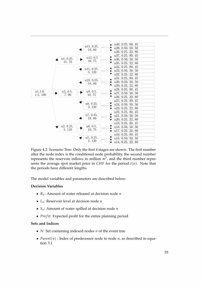
n1,1.0, 1.5, 100
n5, 0.25, 3, 120
n6, 0.5, 10, 75
n7, 0.25, 18, 60
n8, 0.25, 3, 120
n9, 0.5, 10, 75
n10, 0.25, 18, 60
n11, 0.25, 3, 120
n12, 0.510, 75
n13, 0.25, 18, 60
n3, 0.5, 7, 90
n4, 0.25, 15, 70
n2, 0.25, 5, 110
n14, 0.25, 22, 80n15, 0.50, 50, 50n16, 0.25, 80, 45n17, 0.25, 22, 80n18, 0.50, 50, 50n19, 0.25, 80, 45n20, 0.25, 22, 80n21, 0.50, 50, 50n22, 0.25, 80, 45n23, 0.25, 22, 80n24, 0.50, 50, 50n25, 0.25, 80, 45n26, 0.25, 22, 80n27, 0.50, 50, 50n28, 0.25, 80, 45n29, 0.25, 22, 80n30, 0.50, 50, 50n31, 0.25, 80, 45n32, 0.25, 22, 80n33, 0.50, 50, 50n34, 0.25, 80, 45n35, 0.25, 22, 80n36, 0.50, 50, 50n37, 0.25, 80, 45n38, 0.25, 22, 80n39, 0.50, 50, 50n40, 0.25, 80, 45
Figure 4.2: Scenario Tree: Only the first 4 stages are shown. The first numberafter the node index is the conditional node probability, the second numberrepresents the reservoir inflows in million m3, and the third number repre-sents the average spot market price in CHF for the period t(n). Note thatthe periods have different lengths.
The model variables and parameters are described below:
Decision Variables
• Rn: Amount of water released at decision node n
• Ln: Reservoir level at decision node n
• Sn: Amount of water spilled at decision node n
• Pro f it: Expected profit for the entire planning period
Sets and Indices
• N: Set containing indexed nodes n of the event tree
• Parent(n) : Index of predecessor node to node n, as described in equa-tion 3.1
55

4. Release Model
• t(n) : Index of the time period that corresponds to node n, as describedin equation 3.5
• Nend : Set containing all nodes that correspond to the last stage: that is,where t(n) = t6
Parameters
• In: Reservoir inflow at node n
• Prn: Electricity price at node n
• Pn: Probability of being at node n
• cs: Spill over costs
• Lmax: Maximum reservoir capacity
• Lmin: Minimum reservoir capacity
• Lend: Reservoir level at end of model horizon
• Lstart: Initial reservoir level at beginning of model horizon
• Rmax,t: Maximum reservoir release during period t
• ε: Energy equivalent value of water: how much electricity can be pro-duced per amount of water
• Tt: Years from now until time period t
The mathematical formulation to maximize the expected profit is given by:
MaximizePro f it = ∑
n∈NPn(1 + d)−Tt(n) (PrnRnε− csSn) , (4.2)
Subject to
Ln1 = Lstart + In1 − Rn1 − Fn1, (4.3)Ln = LParent(n) + In − Rn − Fn ∀n ∈ N \ n = n1, , (4.4)
0 ≤ Rn ≤ Rmax,t(n) ∀n ∈ N, (4.5)
0 ≤ Ln ≤ Lmax ∀n ∈ N, (4.6)Ln = Lend,n ∀n ∈ Nend, (4.7)
0 ≤ Sn ∀n ∈ N (4.8)
The profit function 4.2 represents the expected profit by summing up thenodal profits weighted by their particular node probabilities Pn. There are nodirect variable costs of production. However, spill-over costs in each nodeare represented through the term csSn in the profit function. Furthermore,
56

each cash flow is adapted with the help of the discount interest rate d to dis-count all cash flows to the present value (PV). The interest rate d is adaptedfor periods of unequal lengths [2].
The initial reservoir level is given by LStart. Equation 4.3 represents the physi-cal reservoir balance for the deterministic first stage. Equation 4.4 representsthe physical reservoir balance for the other nodes, whereas the function Par-ent(n) describes the mapping of each node to its predecessor node.
To avoid end-horizon effects, a target reservoir level, Lend, was specified forall the nodes, n, at the end of the model horizon. The numerical values ofthe constraints correspond approximately to the Grande-Dixence reservoir,assuming that only the power plant Bieudron is used for electricity genera-tion and that pumping facilities are ignored.
Constraints: Value:Lmax: 400 million m3
Lmin: 40 million m3
Lend: 0.5·Lmax = 200 million m3
ε: 4618 MWh per million m3
Table 4.1: Physical Constraints
The maximum release capacity, Rmax, of the power plant Bieudron is givenby 6.48 million m3/s. Hence the maximum release capacity per time periodRmax,t is given by d · Rmax, whereas d is the duration of time period t.
Release Constraints for t: Duration of d: Value:Rmax,t1: 1 d 6.48 million m3
Rmax,t2: 7 d 45.36 million m3
Rmax,t3: 7 d 45.36 million m3
Rmax,t4: 70 d 453.6 million m3
Rmax,t5: 70 d 453.6 million m3
Rmax,t6: 210 d 1360.8 million m3
Table 4.2: Physical Constraints
In reality, the model would be applied dynamically meaning that the oper-ator just uses the first stage decision and then reruns the model based onnew market information. In other words, it is necessary to generate a newscenario tree each day, such as the one described in Figure 4.2, which servesas input data for the model. This guarantees that decisions are always takenbased on the latest price and inflow expectations [2].
57

4. Release Model
4.1 Risk aversion
The example below illustrates different attitudes towards risk:
Example: A gambler has two alternatives:
• Alternative 1: He can play safe and receive 50 CHF with 100 percentcertainty.
• Alternative 2: He can gamble and receive either 0 CHF or 100 CHFwith 50 percent certainty of each occurring.
For a risk-neutral player, both alternatives are equivalent as they both offerthe same expected payoff, namely 50 CHF. On the other hand, a risk-averseplayer would also accept a guaranteed payment of less than 50 CHF, ratherthan take alternative 2 and risk receiving no payment at all. Finally, the risk-seeking player, who hopes to win 100 CHF, would only take the guaranteedpayment if he received more than 50 CHF, as he prefers to take the gamble.
In the hydro scheduling model described above, the operator was assumedto have a risk-neutral attitude towards his production. The objective function4.2, which is to be maximized, implies that the operator’s utility is directlyproportional to the expected profit.
However, considering a risk-averse producer, the model can be adapted toaccount for the operator’s risk preferences. Instead of maximizing the ex-pected profits, we would maximize a utility function that, based on the oper-ator’s risk attitude, represents the operator’s perceived satisfaction with theexpected outcome.
The isoelastic function for utility is used to describe a decision-maker’s utilityin terms of a specific economic variable: in our case, this is the operator’sprofit π. The utility function is given by:
u(π) =
{π1−γ−1
1−γ , if γ is unequal to 1
ln π, if γ is equal to 1(4.9)
Where γ is a measure of the operator’s degree of risk aversion; if γ is equalto 0, the operator is risk neutral, a positive γ implies risk aversion and anegative γ represents risk-seeking behavior.
The graph on the next page illustrate the utility function u(π) for differentvalues of γ.
58

4.1. Risk aversion
Figure 4.3: Risk-averse utility function for different values of γ
The formulation of our hydro scheduling optimization for a risk-averse pro-ducer (γ ≥ 0), which maximizes the expected utility rather than the expectedprofit, is given by:
MaximizeExpected Utility = ∑
n∈Nend
Pnu(πn), (4.10)
Whereas
πn = πParent(n) + (1 + d)−Tt(n) (PrnRnε− csSn) (4.11)
πn represents the discounted present value (PV) of the cumulative profitat each node n as described in 4.11, and u(πn) is the utility function asspecified in equation 4.9 having πn as an argument. Because the cumulativeprofits are used at the leaf nodes (or scenarios), we simply sum over thenodes that correspond to the last stage (n ∈ Nend). The constraints are thesame as those described in equations 4.3-4.8 in the original model.
59

4. Release Model
4.2 GAMS Implementation
The GAMS implementation code for our model is attached in Appendix A.5:the treegeneration tool was used to create the scenario tree structure. Theoperator was allowed to specify his risk preferences γ with the parametergamma. In the risk-neutral case, where gamma = 0, the objective function islinear as we simply maximize the expected profits. In the risk-averse case,however, where gamma > 0, the objective function becomes nonlinear as theexpected utility of the profits is maximized according to the utility functionspecified in equation 4.9. Therefore, GAMS will be advised to use a non-linear solver NLP. The model is a basic extension of the Clear Lake damexample discussed earlier.
Special attention must be paid to the scaling, as most NLP solvers may notfind an optimal or even feasible solution if the involved variables are poorlyscaled. We know from the deterministic optimization that the yearly profitsare of order 108, so we will introduce a parameter piscale = 10−8 to scale thevariable Profit(t,n) that represents the cumulative profit πn.
Furthermore, it is useful to set a starting point in order to help the solverfind a solution: the GAMS default starting point is zero, which is often nota good choice. The statement Profit.L(t,n) = 1 sets the starting level to 1. Asour utility function is of the form log x or
√x, it makes sense to set a lower
level for the profit variable (Profit(t,n).LO = 0.001) to ensure that all functionscan be properly evaluated [5].
60

4.3. Results and Discussion
4.3 Results and Discussion
As mentioned above, evaluating the real performance of the model wouldsimply involve using the first-stage release decision and then rerunning themodel based on the latest inflow and price expectations. In reality, thiswould require us to adapt the scenario tree described in Figure 4.2 on a dailybasis. Having applied the model in a dynamic way during a certain timeperiod, we could then evaluate the actual performance by comparing theresults to the best possible outcome, which can be derived in a deterministicoptimization. Of course, the performance would fundamentally depend onthe quality of the price and inflow forecasts.
However, to simplify matters, our evaluation is limited to a description ofthe model outputs for different inflow and price predictions and changes inthe system’s constraints.
Sensitivity of first-stage decision to expected prices and inflows:
Using different scenario trees as input data, various simulations support theintuition that the first-stage release decision fundamentally depends on thedifference between the price level of the first stage and the price level of thefuture stages.
If the prices for the future stages are expected to be high in relation to thecurrently observed day-ahead price for the first stage, the generation is lowor even zero in the first period. On the other hand, if the currently observedday-ahead price is high compared to the future stages, generation is maxi-mized in the first stage.
The described effect becomes particularly apparent if the prices of the sec-ond stage are significantly different from the first stage, as the probability ofreaching such a state is relatively high.
The same behavior can be observed for the reservoir inflows. If the inflowsin the first period are relatively high compared to the expected inflows ofthe following stages, generation is increased in the first stage. However, thesensitivity of the first stage decision to high inflows is not as strong as thesensitivity towards high prices. This is due to the different lengths of thetime periods; if inflows are high in the first period, which involves just oneday, there is no urgent need to release water as the daily inflow is usuallytoo small compared to the reservoir’s volume to cause a spill-over.
The first-stage decision also depends on the initial reservoir level Lstart; if thereservoir is almost full at the beginning of the model horizon, the first-stagedecision will increase generation, even if prices are comparatively low withrespect to future periods.
Of course, there are also interlocking effects among reservoir inflows, priceexpectations and boundary conditions. For example, if the prices are ex-
61

4. Release Model
pected to be very high at one stage and the reservoir inflows have also beenhigh up to this stage, the model will risk a spill-over (depending on the spill-over costs) at prior stages in order to profit from the interplay between highprices and a fully charged reservoir.
Expected profit in relation to maximum release capacity:
The simulations show that the expected profit increases if the model’s dailymaximum release capacity Rmax is changed. This seems reasonable giventhat the bigger the release capacity, the more flexibility is available to storethe water in the hope of more favorable future prices without risking a spillover. Figure 4.4 illustrates the exact relationship between the expected profitand the daily maximum release capacity Rmax. If the maximum release capacityis equal to zero, the expected profit will be negative, as the entire reservoircontent must be spilled over, which incurs spill-over costs. As Rmax increases,the expected profit increases as well. However, at a certain release capacity,the expected profit reaches a maximum because there is no more additionalbenefit for an increased flexibility. The reservoir operator already has theoptimal release capacity (Bieudron can release up to 6.48 million m3 per day).The averaged expected profit was calculated on the basis of five differentscenario trees.
0 0.5 1 1.5 2 2.5 3 3.5 4 4.5 5 5.5 6 6.5 7 7.5 8
-400000000
-300000000
-200000000
-100000000
0
100000000
200000000
300000000
Averaged Expected Profit
Maximum Release Capacity in million m^3
Figure 4.4: Relationship between expected profit and maximum release ca-pacity.
62
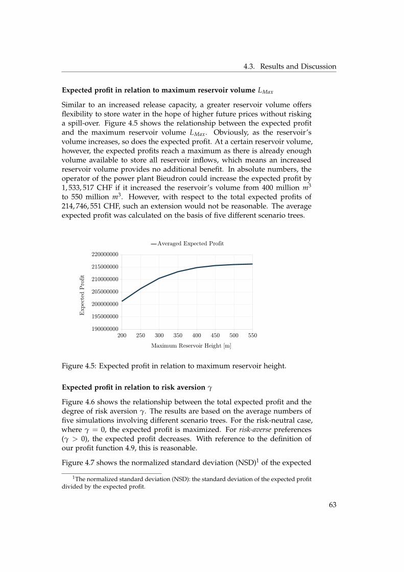
4.3. Results and Discussion
Expected profit in relation to maximum reservoir volume LMax
Similar to an increased release capacity, a greater reservoir volume offersflexibility to store water in the hope of higher future prices without riskinga spill-over. Figure 4.5 shows the relationship between the expected profitand the maximum reservoir volume LMax. Obviously, as the reservoir’svolume increases, so does the expected profit. At a certain reservoir volume,however, the expected profits reach a maximum as there is already enoughvolume available to store all reservoir inflows, which means an increasedreservoir volume provides no additional benefit. In absolute numbers, theoperator of the power plant Bieudron could increase the expected profit by1, 533, 517 CHF if it increased the reservoir’s volume from 400 million m3
to 550 million m3. However, with respect to the total expected profits of214, 746, 551 CHF, such an extension would not be reasonable. The averageexpected profit was calculated on the basis of five different scenario trees.
200 250 300 350 400 450 500 550190000000
195000000
200000000
205000000
210000000
215000000
220000000
Averaged Expected Profit
Maximum Reservoir Height [m]
Exp
ecte
d P
rofit
Figure 4.5: Expected profit in relation to maximum reservoir height.
Expected profit in relation to risk aversion γ
Figure 4.6 shows the relationship between the total expected profit and thedegree of risk aversion γ. The results are based on the average numbers offive simulations involving different scenario trees. For the risk-neutral case,where γ = 0, the expected profit is maximized. For risk-averse preferences(γ > 0), the expected profit decreases. With reference to the definition ofour profit function 4.9, this is reasonable.
Figure 4.7 shows the normalized standard deviation (NSD)1 of the expected
1The normalized standard deviation (NSD): the standard deviation of the expected profitdivided by the expected profit.
63

4. Release Model
0 0.5 1 1.5 2 2.5 3 3.5 4 4.5220000000
225000000
230000000
235000000
240000000
Expected Profit - Risk Aversion
Averaged Expected Profit
Risk Aversion: Gamma
Exp
ecte
d P
rofit
Figure 4.6: Relationship between expected profit and risk aversion factor γ.
profit in relation to the degree of risk aversion γ. Taking the NSD as an in-tuitive risk indicator, the risk (normalized standard deviation) decreases forrisk-averse preferences (γ > 0), which is consistent with our expectations.
However, the NSD in our simulations is rather small, so the relative reduc-tion from the risk-neutral case (γ = 0 where the NSD is approximately 2percent) to the risk-averse case (γ = 4.5 where the NSD is approximately1.65 percent) seems to be of minor relevance. The small standard deviationsare probably due to the underlying scenario trees used in our simulations.It would be interesting to run our model based on a representative numberof realistic scenario trees to further investigate the effect of the risk aversionfactor γ on the expected profit and the standard deviation. However, sub-stantial modeling of future electricity market prices and reservoir inflows isbeyond the scope of this thesis. Figure 4.7 shows the average results for fivedifferent scenario trees.
64
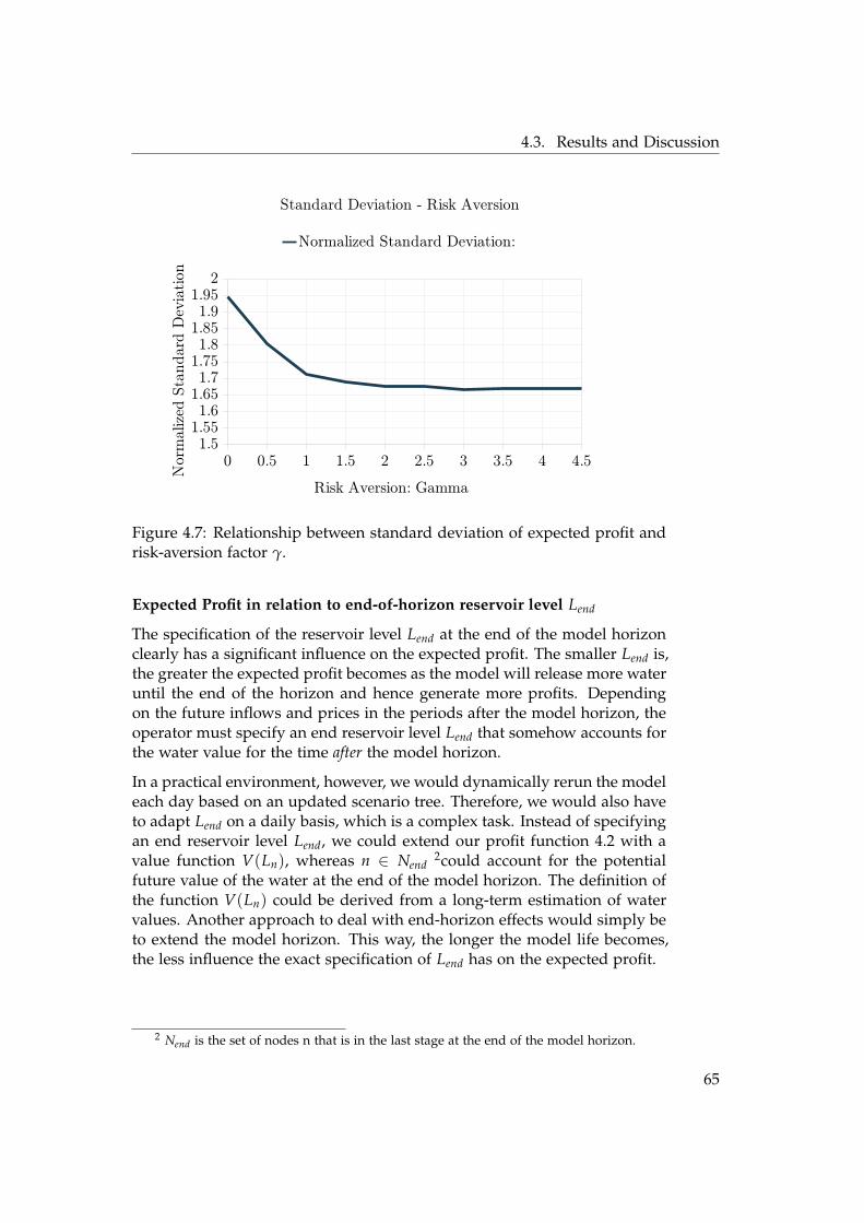
4.3. Results and Discussion
0 0.5 1 1.5 2 2.5 3 3.5 4 4.51.5
1.551.6
1.651.7
1.751.8
1.851.9
1.952
Standard Deviation - Risk Aversion
Normalized Standard Deviation:
Risk Aversion: Gamma
Nor
mal
ized
Sta
ndard
Dev
iation
Figure 4.7: Relationship between standard deviation of expected profit andrisk-aversion factor γ.
Expected Profit in relation to end-of-horizon reservoir level Lend
The specification of the reservoir level Lend at the end of the model horizonclearly has a significant influence on the expected profit. The smaller Lend is,the greater the expected profit becomes as the model will release more wateruntil the end of the horizon and hence generate more profits. Dependingon the future inflows and prices in the periods after the model horizon, theoperator must specify an end reservoir level Lend that somehow accounts forthe water value for the time after the model horizon.
In a practical environment, however, we would dynamically rerun the modeleach day based on an updated scenario tree. Therefore, we would also haveto adapt Lend on a daily basis, which is a complex task. Instead of specifyingan end reservoir level Lend, we could extend our profit function 4.2 with avalue function V(Ln), whereas n ∈ Nend
2could account for the potentialfuture value of the water at the end of the model horizon. The definition ofthe function V(Ln) could be derived from a long-term estimation of watervalues. Another approach to deal with end-horizon effects would simply beto extend the model horizon. This way, the longer the model life becomes,the less influence the exact specification of Lend has on the expected profit.
2 Nend is the set of nodes n that is in the last stage at the end of the model horizon.
65

4. Release Model
Conclusion (Summary)
This thesis has provided step-by-step instructions for using the frameworkof stochastic programming to approach hydropower production scheduling.The paper focused especially on the practical implementation with the alge-braic modeling language GAMS. As shows the first chapter, there is usuallya significant gap between the actual profit generated by a hydropower op-erator and the theoretical maximum profit the operator could have gainedif he had perfect information about reservoir inflows and electricity pricesat the beginning of the year. This generates the need to develop effectiveproduction scheduling models.
The second chapter showed how to use stochastic recourse models to solvean optimization problem that involves decision making under uncertainty.The basic example provided was an adapted version of the Clear Lake model,which is part of the GAMS model library. Based on our future expectationsabout the evolution of the reservoir inflows, we illustrated two different ap-proaches to describe a stochastic scenario tree: namely a node-based notationand a scenario-based notation. Each approache offers specific advantages. Anode-based model can be solved slightly faster than a scenario-based model,while the solution report of a scenario-based model may be interpreted in astraight-forward manner.
The third chapter discussed computational issues concerning stochastic pro-gramming and showed how the model execution time rises exponentiallywith each additional time step added to the model horizon. We showedhow the performance of GAMS is limited in creating large scenario treesby assigning memberships to dynamic sets. Therefore, the thesis introducesa treegeneration tool written in the programming language C++, which sig-nificantly speeds up the GAMS model generation phase. By outsourcing thegeneration of the scenario tree to the treegeneration tool, we were able to usemuch larger stochastic multi-stage models than would have been possibleby creating the scenario tree structure within GAMS.
This chapter also showed how to use the scenario reduction tool SCENREDfrom the GAMS standard model library, which scales down the size of anode-based multi-stage model, thereby attempting to reduce the model solu-tion time. However, we conclude that SCENRED fails to speed up the totalsolution time of large multi-stage models, as the reduction time is greaterthan the time gain that results from the reduced scenario tree.
Finally, the fourth chapter extended the Clear Lake example to a more re-alistic release model (”Release Model”) that determines the optimal reservoirrelease decision for the following production day with respect to future in-flow and price expectations.
The analysis showed that the Release Model produces reasonable outputs for
66

4.3. Results and Discussion
a range of different input parameters and is suitable for quantifying the in-fluence of these parameters on the expected profit and the first-stage releasedecision. Furthermore, the Release Model can be used to analyze the effectof different risk attitudes on the production schedule. Based on five differ-ent scenario trees as input data, the analysis showed that both the expectedprofit and the normalized standard deviation of the expected profit werereduced if risk-aversion was incorporated into the model.
However, some aspects remain to be developed if the Release Model is tobecome more realistic. For example, the model could be expanded to amulti-reservoir system that includes pumping facilities, or it could take intoaccount the nonlinear relationship between water release and power gener-ation that was discussed in the first chapter. Furthermore, the Release Modelpresented in this paper included six time periods, resulting in 243 differentstochastic scenarios: this allowed for three stochastic realizations per deci-sion node. Depending on the available price and inflow forecasts, it wouldbe interesting to compare the relative performance among models that havedifferent model lives, including different numbers of stochastic realizationsper decision node.
Moreover, the thesis did not evaluate the actual performance of our ReleaseModel (which would result from the actual yearly profit generated by apply-ing the model for production scheduling). Such computations would haveto be based on daily generated scenario trees describing the latest inflowand price expectations. This would be beyond the scope of this thesis.
67


Appendix A
Appendix
All models used in this thesis and the treegeneration tool can be downloadedunder:
http://dl.dropbox.com/u/24263007/Treegen.zip
69
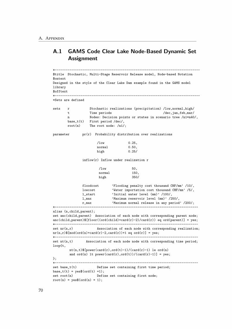
A. Appendix
A.1 GAMS Code Clear Lake Node-Based Dynamic SetAssignment
*-------------------------------------------------------------------------------
$title Stochastic, Multi-Stage Reservoir Release model, Node-based Notation
$ontext
Designed in the style of the Clear Lake Dam example found in the GAMS model
library
$offtext
*-------------------------------------------------------------------------------
*Sets are defined
sets r Stochastic realizations (precipitation) /low,normal,high/
t Time periods /dec,jan,feb,mar/
n Nodes: Decision points or states in scenario tree /n1*n40/,
base_t(t) First period /dec/,
root(n) The root node: /n1/;
parameter pr(r) Probability distribution over realizations
/low 0.25,
normal 0.50,
high 0.25/
inflow(r) Inflow under realization r
/low 50,
normal 150,
high 350/
floodcost ’Flooding penalty cost thousand CHF/mm’ /10/,
lowcost ’Water importation cost thousand CHF/mm’ /5/,
l_start ’Initial water level (mm)’ /100/,
l_max ’Maximum reservoir level (mm)’ /250/,
r_max ’Maximum normal release in any period’ /200/;
*------------------------------------------------------------------------------
alias (n,child,parent);
set anc(child,parent) Association of each node with corresponding parent node;
anc(child,parent)$[floor((ord(child)+card(r)-2)/card(r)) eq ord(parent)] = yes;
*------------------------------------------------------------------------------
set nr(n,r) Association of each node with corresponding realization;
nr(n,r)$[mod(ord(n)+card(r)-2,card(r))+1 eq ord(r)] = yes;
*------------------------------------------------------------------------------
set nt(n,t) Association of each node node with corresponding time period;
loop{t,
nt(n,t)$[power(card(r),ord(t)-1)/(card(r)-1) le ord(n)
and ord(n) lt power(card(r),ord(t))/(card(r)-1)] = yes;
};
*------------------------------------------------------------------------------
set base_t(t) Define set containing first time period;
base_t(t) = yes$(ord(t) =1);
set root(n) Define set containing first node;
root(n) = yes$(ord(n) = 1);
70

A.1. GAMS Code Clear Lake Node-Based Dynamic Set Assignment
*-------------------------------------------------------------------------------
* Calculate water inflows at each node:
parameter n_inflow(n) Water inflow at each node;
n_inflow(n)$[not root(n)] = sum{(nr(n,r)),inflow(r)};
*-------------------------------------------------------------------------------
* Calculate water inflows at each node:
parameter n_prob(n) Probability of being at a node;
n_prob(root) = 1;
loop {anc(child,parent),
n_prob(child) = sum {nr(child,r), pr(r)} * n_prob(parent);};
*-------------------------------------------------------------------------------
* Model logic:
variable EC ’Expected costs’;
positive variable L(n,t) ’Reservoir water level -- EOP’
Release(n,t) ’Normal release of water (mm)’
F(n,t) ’Floodwater released (mm)’
Z(n,t) ’Water imports (mm)’;
equations ecdef, ldef;
ecdef..
EC =e= sum {nt(n,t),n_prob(n)*[floodcost*F(n,t)+lowcost*Z(n,t)]};
ldef(nt(n,t))$[not root(n)]..
L(n,t) =e= sum{anc(n,parent),l(parent,t-1)}+n_inflow(n)+Z(n,t)-Release(n,t)-F(n,t);
Release.up(n,t) = r_max;
L.up(n,t) = l_max;
L.fx(n,base_t) = l_start;
*-------------------------------------------------------------------------------
model mincost / ecdef, ldef /;
solve mincost using LP minimizing EC;
*-------------------------------------------------------------------------------
71

A. Appendix
A.2 GAMS Code Clear Lake Node-Based with tree-gen.exe
*-------------------------------------------------------------------------------
$title Stochastic, Multi-Stage Reservoir Release model, Node-based Notation
$ontext
Designed in the style of the Clear Lake Dam example found in the GAMS model
library
$offtext
*-------------------------------------------------------------------------------
*Sets are defined
sets r Stochastic realizations (precipitation) /low,normal,high/,
t Time periods /dec,jan,feb,mar/;
parameters pr(r) Probability distribution over realizations
/low 0.25,
normal 0.50,
high 0.25/
inflow(r) Inflow under realization r
/low 50,
normal 150,
high 350/
floodcost ’Flooding penalty cost thousand CHF/mm’ /10/,
lowcost ’Water importation cost thousand CHF/mm’ /5/,
l_start ’Initial water level (mm)’ /100/,
l_max ’Maximum reservoir level (mm)’ /250/,
r_max ’Maximum normal release in any period’ /200/;
*-------------------------------------------------------------------------------
* Unload the time and realization sets "t", "r" and the realization specific
* probabilities "pr" into a GDX file and start treegeneration tool:
$gdxout cl_in.gdx
$unload t=time_set r=realization_set pr=prob
$gdxout
$call treegen.exe cl_in.gdx cl_out.gdx "%gams.sysdir%\"
*-------------------------------------------------------------------------------
* Read data structures describing the node-based tree:
$gdxin cl_out.gdx
set n Nodes set;
$load n=n
set anc(n,n) Predecessor-mapping for node set;
$load anc=anc
set nr(n,r) Node-realization-mapping;
$load nr=nr
set nt(n,t) Node-time-mapping;
$load nt=nt
parameter n_prob(n) Nodal probabilities;
72
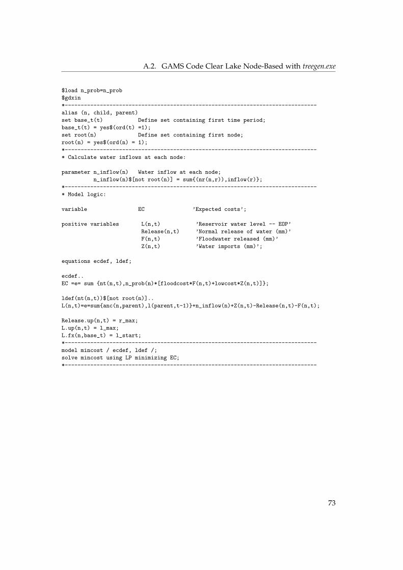
A.2. GAMS Code Clear Lake Node-Based with treegen.exe
$load n_prob=n_prob
$gdxin
*-------------------------------------------------------------------------------
alias (n, child, parent)
set base_t(t) Define set containing first time period;
base_t(t) = yes$(ord(t) =1);
set root(n) Define set containing first node;
root(n) = yes$(ord(n) = 1);
*-------------------------------------------------------------------------------
* Calculate water inflows at each node:
parameter n_inflow(n) Water inflow at each node;
n_inflow(n)$[not root(n)] = sum{(nr(n,r)),inflow(r)};
*-------------------------------------------------------------------------------
* Model logic:
variable EC ’Expected costs’;
positive variables L(n,t) ’Reservoir water level -- EOP’
Release(n,t) ’Normal release of water (mm)’
F(n,t) ’Floodwater released (mm)’
Z(n,t) ’Water imports (mm)’;
equations ecdef, ldef;
ecdef..
EC =e= sum {nt(n,t),n_prob(n)*[floodcost*F(n,t)+lowcost*Z(n,t)]};
ldef(nt(n,t))$[not root(n)]..
L(n,t)=e=sum{anc(n,parent),l(parent,t-1)}+n_inflow(n)+Z(n,t)-Release(n,t)-F(n,t);
Release.up(n,t) = r_max;
L.up(n,t) = l_max;
L.fx(n,base_t) = l_start;
*-------------------------------------------------------------------------------
model mincost / ecdef, ldef /;
solve mincost using LP minimizing EC;
*-------------------------------------------------------------------------------
73

A. Appendix
A.3 GAMS Code Clear Lake Scenario-Based with tree-gen.exe
*-------------------------------------------------------------------------------
$title Stochastic, Multi-Stage Reservoir Release model, Scenario-Based Notation
$ontext
Designed in the style of the Clear Lake Dam example found in the GAMS model
library
$offtext
*-------------------------------------------------------------------------------
*Sets are defined
sets r Stochastic realizations (precipitation) /low,normal,high/,
t Time periods /dec,jan,feb,mar/;
parameter pr(r) Probability distribution over realizations
/low 0.25,
normal 0.50,
high 0.25/
inflow(r) Inflow under realization r
/low 50,
normal 150,
high 350/
floodcost ’Flooding penalty cost thousand CHF/mm’ /10/,
lowcost ’Water importation cost thousand CHF/mm’ /5/,
l_start ’Initial water level (mm)’ /100/,
l_max ’Maximum reservoir level (mm)’ /250/,
r_max ’Maximum normal release in any period’ /200/;
*-------------------------------------------------------------------------------
* Unload the time and realization sets "t", "r" and the realization specific
* probabilities "pr" into a GDX file and start treegeneration tool:
$gdxout cl_in.gdx
$unload t=time_set r=realization_set pr=prob
$gdxout
$call treegen.exe cl_in.gdx cl_out.gdx "%gams.sysdir%\"
*-------------------------------------------------------------------------------
* Read data structures describing the scenario-based tree:
$gdxin cl_out.gdx
set s Scenarios - Leaves in the event tree;
$load s=s
set eq(s,t) Equilibrium points - Equivalent to nodes;
$load eq=eq
set str(s,t,r) Association of scenarios with realizations;
$load str=str
parameter o(s,t) Offset pointer;
$load o=offset
parameter eq_prob(s,t) Probability to reach equilibrium point eq;
74
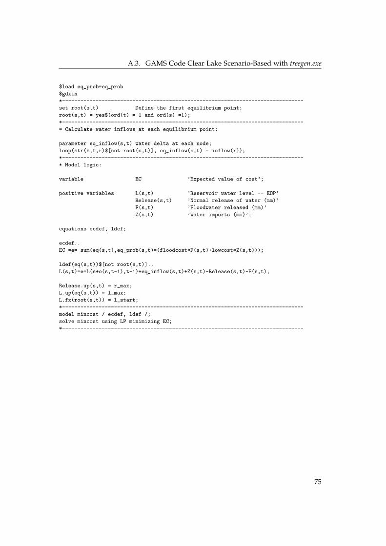
A.3. GAMS Code Clear Lake Scenario-Based with treegen.exe
$load eq_prob=eq_prob
$gdxin
*-------------------------------------------------------------------------------
set root(s,t) Define the first equilibrium point;
root(s,t) = yes$(ord(t) = 1 and ord(s) =1);
*-------------------------------------------------------------------------------
* Calculate water inflows at each equilibrium point:
parameter eq_inflow(s,t) water delta at each node;
loop(str(s,t,r)$[not root(s,t)], eq_inflow(s,t) = inflow(r));
*-------------------------------------------------------------------------------
* Model logic:
variable EC ’Expected value of cost’;
positive variables L(s,t) ’Reservoir water level -- EOP’
Release(s,t) ’Normal release of water (mm)’
F(s,t) ’Floodwater released (mm)’
Z(s,t) ’Water imports (mm)’;
equations ecdef, ldef;
ecdef..
EC =e= sum(eq(s,t),eq_prob(s,t)*(floodcost*F(s,t)+lowcost*Z(s,t)));
ldef(eq(s,t))$[not root(s,t)]..
L(s,t)=e=L(s+o(s,t-1),t-1)+eq_inflow(s,t)+Z(s,t)-Release(s,t)-F(s,t);
Release.up(s,t) = r_max;
L.up(eq(s,t)) = l_max;
L.fx(root(s,t)) = l_start;
*-------------------------------------------------------------------------------
model mincost / ecdef, ldef /;
solve mincost using LP minimizing EC;
*-------------------------------------------------------------------------------
75
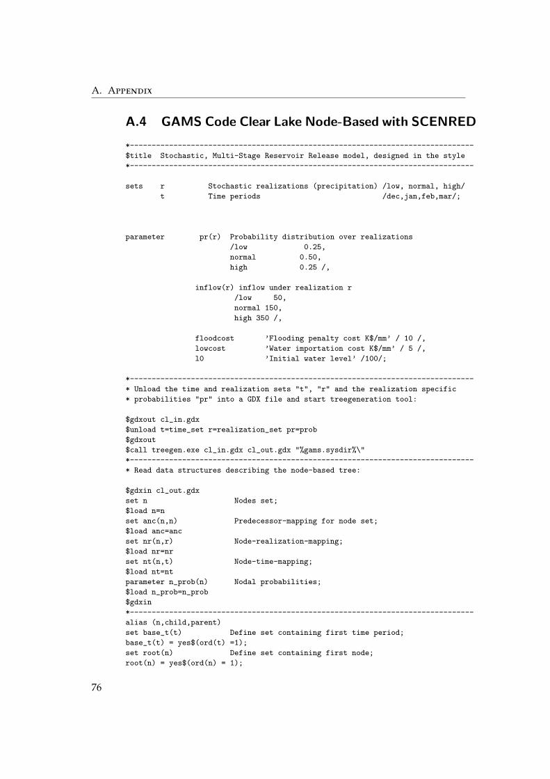
A. Appendix
A.4 GAMS Code Clear Lake Node-Based with SCENRED
*-------------------------------------------------------------------------------
$title Stochastic, Multi-Stage Reservoir Release model, designed in the style
*-------------------------------------------------------------------------------
sets r Stochastic realizations (precipitation) /low, normal, high/
t Time periods /dec,jan,feb,mar/;
parameter pr(r) Probability distribution over realizations
/low 0.25,
normal 0.50,
high 0.25 /,
inflow(r) inflow under realization r
/low 50,
normal 150,
high 350 /,
floodcost ’Flooding penalty cost K$/mm’ / 10 /,
lowcost ’Water importation cost K$/mm’ / 5 /,
l0 ’Initial water level’ /100/;
*-------------------------------------------------------------------------------
* Unload the time and realization sets "t", "r" and the realization specific
* probabilities "pr" into a GDX file and start treegeneration tool:
$gdxout cl_in.gdx
$unload t=time_set r=realization_set pr=prob
$gdxout
$call treegen.exe cl_in.gdx cl_out.gdx "%gams.sysdir%\"
*-------------------------------------------------------------------------------
* Read data structures describing the node-based tree:
$gdxin cl_out.gdx
set n Nodes set;
$load n=n
set anc(n,n) Predecessor-mapping for node set;
$load anc=anc
set nr(n,r) Node-realization-mapping;
$load nr=nr
set nt(n,t) Node-time-mapping;
$load nt=nt
parameter n_prob(n) Nodal probabilities;
$load n_prob=n_prob
$gdxin
*-------------------------------------------------------------------------------
alias (n,child,parent)
set base_t(t) Define set containing first time period;
base_t(t) = yes$(ord(t) =1);
set root(n) Define set containing first node;
root(n) = yes$(ord(n) = 1);
76
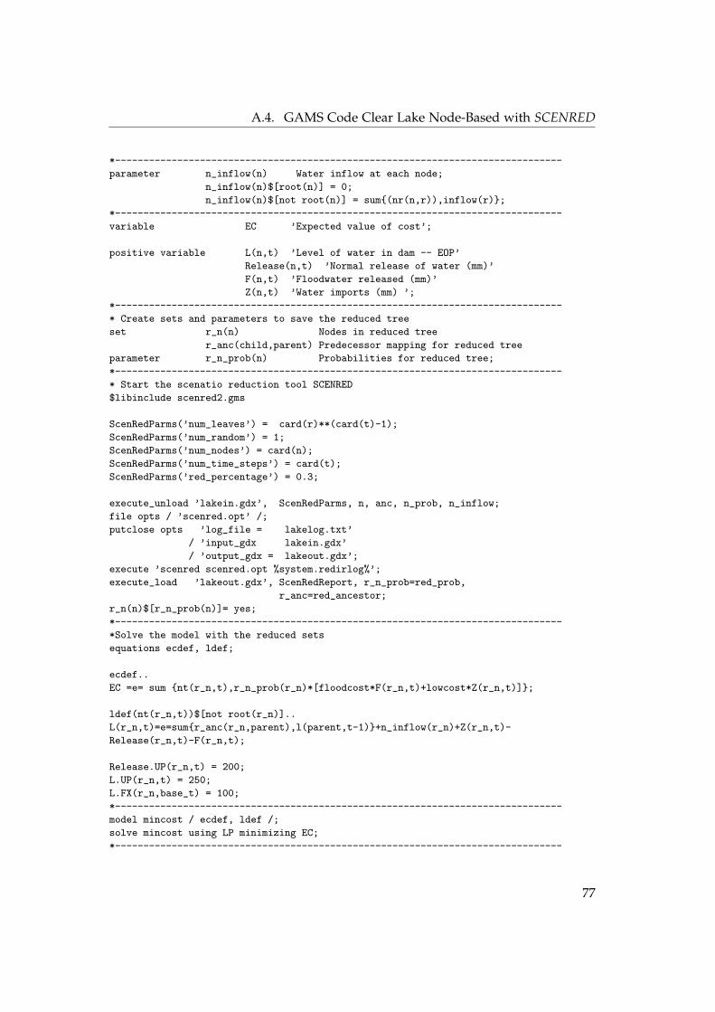
A.4. GAMS Code Clear Lake Node-Based with SCENRED
*-------------------------------------------------------------------------------
parameter n_inflow(n) Water inflow at each node;
n_inflow(n)$[root(n)] = 0;
n_inflow(n)$[not root(n)] = sum{(nr(n,r)),inflow(r)};
*-------------------------------------------------------------------------------
variable EC ’Expected value of cost’;
positive variable L(n,t) ’Level of water in dam -- EOP’
Release(n,t) ’Normal release of water (mm)’
F(n,t) ’Floodwater released (mm)’
Z(n,t) ’Water imports (mm) ’;
*-------------------------------------------------------------------------------
* Create sets and parameters to save the reduced tree
set r_n(n) Nodes in reduced tree
r_anc(child,parent) Predecessor mapping for reduced tree
parameter r_n_prob(n) Probabilities for reduced tree;
*-------------------------------------------------------------------------------
* Start the scenatio reduction tool SCENRED
$libinclude scenred2.gms
ScenRedParms(’num_leaves’) = card(r)**(card(t)-1);
ScenRedParms(’num_random’) = 1;
ScenRedParms(’num_nodes’) = card(n);
ScenRedParms(’num_time_steps’) = card(t);
ScenRedParms(’red_percentage’) = 0.3;
execute_unload ’lakein.gdx’, ScenRedParms, n, anc, n_prob, n_inflow;
file opts / ’scenred.opt’ /;
putclose opts ’log_file = lakelog.txt’
/ ’input_gdx lakein.gdx’
/ ’output_gdx = lakeout.gdx’;
execute ’scenred scenred.opt %system.redirlog%’;
execute_load ’lakeout.gdx’, ScenRedReport, r_n_prob=red_prob,
r_anc=red_ancestor;
r_n(n)$[r_n_prob(n)]= yes;
*-------------------------------------------------------------------------------
*Solve the model with the reduced sets
equations ecdef, ldef;
ecdef..
EC =e= sum {nt(r_n,t),r_n_prob(r_n)*[floodcost*F(r_n,t)+lowcost*Z(r_n,t)]};
ldef(nt(r_n,t))$[not root(r_n)]..
L(r_n,t)=e=sum{r_anc(r_n,parent),l(parent,t-1)}+n_inflow(r_n)+Z(r_n,t)-
Release(r_n,t)-F(r_n,t);
Release.UP(r_n,t) = 200;
L.UP(r_n,t) = 250;
L.FX(r_n,base_t) = 100;
*-------------------------------------------------------------------------------
model mincost / ecdef, ldef /;
solve mincost using LP minimizing EC;
*-------------------------------------------------------------------------------
77

A. Appendix
A.5 GAMS Code Release model
*-------------------------------------------------------------------------------
$title Stochastic, Multi-Stage Reservoir Release model
*-------------------------------------------------------------------------------
sets r Stochastic realizations (inflow and price) /r1, r2, r3/
t Time periods /t1,t2,t3,t4,t5,t6/;
*-------------------------------------------------------------------------------
Parameter pr(r) Probability distribution /
r1 0.25,
r2 0.50,
r3 0.25/;
*-------------------------------------------------------------------------------
* Unload the time and realization sets "t", "r" and the realization specific
* probabilities "pr" into a GDX file and start treegeneration tool:
$gdxout cl_in.gdx
$unload t=time_set r=realization_set pr=prob
$gdxout
$call treegen.exe cl_in.gdx cl_out.gdx "%gams.sysdir%\"
*-------------------------------------------------------------------------------
* Read data structures describing the node-based tree:
$gdxin cl_out.gdx
set n Nodes set;
$load n=n
set anc(n,n) Predecessor-mapping for node set;
$load anc=anc
set nr(n,r) Node-realization-mapping;
$load nr=nr
set nt(n,t) Node-time-mapping;
$load nt=nt
parameter n_prob(n) Nodal probabilities;
$load n_prob=n_prob
$gdxin
*-------------------------------------------------------------------------------
set base_t(t) First period;
base_t(t)$(ord(t)=1) = yes;
set last_period(t) Last time period;
last_period(t)$(ord(t) =card(t)) = yes;
set root(n) First decision node;
root(n)$(ord(n)=1)=yes;
alias (n,child,parent);
set s scenarios /s1*s243/;
*-------------------------------------------------------------------------------
set last_stage(n,t) Set containing decision nodes at the last stage;
scalar tmp1;
tmp1 = sum(t,power(card(r),ord(t)-1)) - power(card(r),card(t)-1);
last_stage(n,t)$[ord(n) gt tmp1 and (ord(t) eq card(t))] = yes;
*-------------------------------------------------------------------------------
set sn(n,s) linking of each scenario to its final node;
scalar tmp1;
tmp1 = sum(t,power(card(r),ord(t)-1)) - power(card(r),card(t)-1);
78

A.5. GAMS Code Release model
sn(n,s)$[ord(s) = (ord(n) - tmp1)] = yes;
*-------------------------------------------------------------------------------
Parameter duration(t) Duration of time period t in hours
/t1 1
t2 7
t3 7
t4 70
t5 70
t6 210/;
Parameter discount(t) Interest rate for period t
/t1 1
t2 0.999465
t3 0.998531
t4 0.993409
t5 0.984157
t6 0.965939/;
Table inflow_t(t,r) Changes in reservoir level for each season million [m^3]
r1 r2 r3
t2 1 2 3
t3 2 3 4
t4 22 33 40
t5 30 40 50
t6 100 150 300;
Table price_t(t,r) Electricity prices under each scenario per month
r1 r2 r3
t2 90 88 30
t3 90 75 60
t4 80 50 45
t5 70 65 40
t6 60 55 50;
Parameter floodcost Flooding cost per million [m^3] /1000000/,
l_start Initial water level million [m^3] /200/,
inflow_1 Inflow during first period t1 in million [m^3] /0.5/,
price_1 Electricity price during first period t1 per MWh /90/,
l_max Maximum reservoir level million [m^3]’ /400/,
r_max_d Release capacity per day million [m^3]’ /6.48/
e Amount of Energy per MWh /4618/
gamma Risk aversion factor /0/;
Parameter r_max(t) Maximum release per months in million [m^3];
r_max(t) = duration(t)*r_max_d;
*-------------------------------------------------------------------------------
Parameter n_inflow(n) Water inflow at each node;
n_inflow(n) = sum{(nt(n,t),nr(n,r)), inflow_t(t,r)};
n_inflow(n)$[root(n)] = inflow_1;
*-------------------------------------------------------------------------------
Parameter n_price(n) Price at each node;
n_price(n) = sum{(nt(n,t),nr(n,r)), price_t(t,r)};
n_price(n)$[root(n)] = price_1;
*-------------------------------------------------------------------------------
parameter piscale Profit scale factor /1e-8/;
*-------------------------------------------------------------------------------
* Model logic:
79

A. Appendix
Variable Total_Profit Expected Total Profit
U Expected Utility
Profit(n,t) Sum of profits up to node n period t;
Positive variable L(n,t) Reservoir water level at node n period t
Release(n,t) Normal release of water node n period t
F(n,t) Floodwater released node n period t;
*Constraint to avoid end-horizon-effects
L.FX(last_stage) = 200;
*-------------------------------------------------------------------------------
* Assign initial values to help NLP solver find solution
Profit.lo(n,t) = 0.001;
Profit.l(n,t) = 1;
*-------------------------------------------------------------------------------
equations l_first_node, l_node, n_profit_1, n_profit_2, profdef, utility;
*Physical reservoir balance for first node:
l_first_node(nt(n,t))$[root(n)]..
L(n,t) =e= l_start + n_inflow(n) - Release(n,t) - F(n,t);
*Physical reservoir balance for the other nodes
l_node(nt(n,t))$[not root(n)]..
L(n,t) =e= sum{anc(n,parent),l(parent,t-1)}+n_inflow(n)-Release(n,t)-F(n,t);
*Profit function for the first node
n_profit_1(nt(n,t))$[root(n)]..
profit(n,t) =e= piscale*discount(t)*[Release(n,t)*e*n_price(n)-F(n,t)*floodcost];
*Profit function for all the other nodes: Total profit up to node n time t:
n_profit_2(nt(n,t))$[not root(n)]..
profit(n,t) =e= sum{anc(n,parent),profit(parent,t-1)}+piscale*discount(t)*
[Release(n,t)*e*n_price(n)-F(n,t)*floodcost] ;
*Total expected profit
profdef..
Total_Profit =e= sum {last_stage(n,t),n_prob(n)*profit(n,t)};
*Expected Utility
utility..
U =e= sum(last_stage(n,t), n_prob(n)*[(profit(n,t)**(1-gamma)-1)/(1-gamma)]);
*Constraints for Maximum release and reservoir height
Release.up(n,t) = r_max(t);
L.up(n,t) = l_max;
*-------------------------------------------------------------------------------
*model maxprof / l_first_node, l_node, n_profit_1, n_profit_2, profdef/;
*solve maxprof using LP maximizing Total_Profit;
model maxutil / l_first_node, l_node, n_profit_1, n_profit_2, utility/;
solve maxutil using NLP maximizing U;
*-------------------------------------------------------------------------------
*Display results: standard dev:
*Calculate standard deviation;
80

A.5. GAMS Code Release model
parameter standard_dev, expected_profit;
expected_profit= sum{last_stage(n,t),n_prob(n)*(profit.L(n,t)/piscale)};
standard_dev = sqrt((1/(power(card(r),card(t)-1)))*sum(last_stage(n,t),n_prob(n)*
power((expected_profit-(profit.L(n,t)/piscale)),2)));
display standard_dev;
display expected_profit;
*-------------------------------------------------------------------------------
81
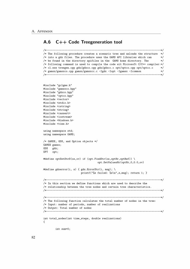
A. Appendix
A.6 C++ Code Treegeneration tool
/*----------------------------------------------------------------------------*/
/* The following procedure creates a scenario tree and unloads the structure */
/* into a gdx files. The procedure uses the GAMS API libraries which can */
/* be found in the directory apifiles in the GAMS home directory. The */
/* following command is used to compile the code wit Microsoft C/C++ compiler:*/
/* cl.exe treegen.cpp gdx/gdxco.cpp gdx/gdxcc.c opt/optco.cpp opt/optcc.c */
/* gamsx/gamsxco.cpp gamsx/gamsxcc.c -Igdx -Iopt -Igamsx -Icommon */
/*----------------------------------------------------------------------------*/
#include "gclgms.h"
#include "gamsxco.hpp"
#include "gdxco.hpp"
#include "optco.hpp"
#include <vector>
#include <stdio.h>
#include <cstring>
#include <string>
#include <cassert>
#include <iostream>
#include <Windows.h>
#include <time.h>
using namespace std;
using namespace GAMS;
/* GAMSX, GDX, and Option objects */
GAMSX gamsx;
GDX gdx;
OPT opt;
#define optSetStrS(os,ov) if (opt.FindStr(os,optNr,optRef)) \
opt.SetValuesNr(optNr,0,0.0,ov)
#define gdxerror(i, s) { gdx.ErrorStr(i, msg); \
printf("%s failed: %s\n",s,msg); return 1; }
/*----------------------------------------------------------------------------*/
/* In this section we define functions which are used to describe the
/* relationship between the tree nodes and certain tree characteristics.
/*----------------------------------------------------------------------------*/
/*----------------------------------------------------------------------------*/
/* The following function calculates the total number of nodes in the tree:
/* Input: number of periods, number of realizations
/* Output: Total number of nodes
/*----------------------------------------------------------------------------*/
int total_nodes(int time_steps, double realizations)
{
int sum=0;
82

A.6. C++ Code Treegeneration tool
int temp1=0;
for(int x=0; x<time_steps; ++x)
{
temp1 = pow(realizations,x);
sum = sum+temp1;
}
return(sum);
}
/*----------------------------------------------------------------------------*/
/* The following function links each node to its corresponding time period
/* Input: node number, number of periods, number of realizations,
/* Output: time period of that node
/*----------------------------------------------------------------------------*/
int node_time_link (int node_number, int time_steps, double realizations)
{
int cperiod=0;
for (int x = 1; x<=time_steps+1; ++x) {
if ((node_number < (pow(realizations,x)/(realizations-1) ) &&
(node_number >= (pow(realizations,x-1)/(realizations-1))))) {
cperiod = x-1;
}
}
return(cperiod);
}
/*----------------------------------------------------------------------------*/
/* The following function links each node to its parent node
/* Input: node number, number of realizations, Output: number of parent node
/*----------------------------------------------------------------------------*/
int parent_node (double node, double realization)
{
int r;
r=floor((node+realization -2)/realization);
return (r);
}
/*----------------------------------------------------------------------------*/
/* The following function maps each node to its corresponding realization
/* Input: node number, number of realizations,
/* Output: realization number of node
/*----------------------------------------------------------------------------*/
int node_realization_map(int node_number, int realizations){
int temp1;
if (node_number == 0) {temp1 = 0;}
else {temp1 = ((node_number+realizations-2)%realizations)+1;}
return(temp1);
}
/*----------------------------------------------------------------------------*/
/* This function converts an integer into a string
83
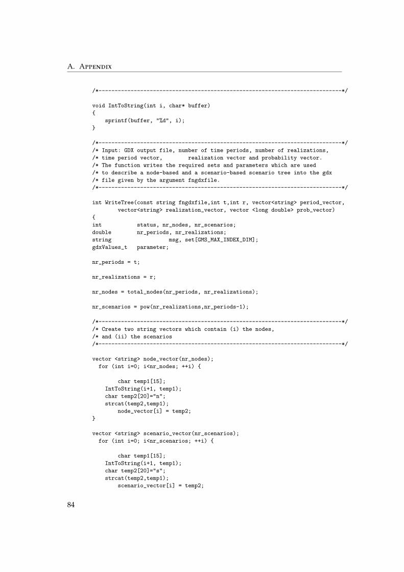
A. Appendix
/*----------------------------------------------------------------------------*/
void IntToString(int i, char* buffer)
{
sprintf(buffer, "%d", i);
}
/*----------------------------------------------------------------------------*/
/* Input: GDX output file, number of time periods, number of realizations,
/* time period vector, realization vector and probability vector.
/* The function writes the required sets and parameters which are used
/* to describe a node-based and a scenario-based scenario tree into the gdx
/* file given by the argument fngdxfile.
/*----------------------------------------------------------------------------*/
int WriteTree(const string fngdxfile,int t,int r, vector<string> period_vector,
vector<string> realization_vector, vector <long double> prob_vector)
{
int status, nr_nodes, nr_scenarios;
double nr_periods, nr_realizations;
string msg, set[GMS_MAX_INDEX_DIM];
gdxValues_t parameter;
nr_periods = t;
nr_realizations = r;
nr_nodes = total_nodes(nr_periods, nr_realizations);
nr_scenarios = pow(nr_realizations,nr_periods-1);
/*----------------------------------------------------------------------------*/
/* Create two string vectors which contain (i) the nodes,
/* and (ii) the scenarios
/*----------------------------------------------------------------------------*/
vector <string> node_vector(nr_nodes);
for (int i=0; i<nr_nodes; ++i) {
char temp1[15];
IntToString(i+1, temp1);
char temp2[20]="n";
strcat(temp2,temp1);
node_vector[i] = temp2;
}
vector <string> scenario_vector(nr_scenarios);
for (int i=0; i<nr_scenarios; ++i) {
char temp1[15];
IntToString(i+1, temp1);
char temp2[20]="s";
strcat(temp2,temp1);
scenario_vector[i] = temp2;
84

A.6. C++ Code Treegeneration tool
}
/*----------------------------------------------------------------------------*/
/* Create a vector that contains the nodal probabilities
/*----------------------------------------------------------------------------*/
vector <long double> node_prob_vector(nr_nodes);
node_prob_vector[0] = 1;
for (int i=2; i<=nr_nodes; ++i){
node_prob_vector[i-1] =
prob_vector[node_realization_map(i,nr_realizations)-1]*
node_prob_vector[parent_node(i,nr_realizations)-1];
}
/*----------------------------------------------------------------------------*/
/* Begin to write GDX file
/*----------------------------------------------------------------------------*/
gdx.OpenWrite(fngdxfile, "GDX Output file", status);
if (status)
gdxerror(status, "gdxOpenWrite");
/*----------------------------------------------------------------------------*/
/* Write node vector as a set into GDX file:
/*----------------------------------------------------------------------------*/
if (0==gdx.DataWriteStrStart("n", "nodes", 1, GMS_DT_SET, 0))
gdxerror(gdx.GetLastError(), "gdxDataWriteStrStart");
for (int i=0; i<nr_nodes; ++i) {
set[0] = node_vector[i];
gdx.DataWriteStr(set, parameter);
}
if (0==gdx.DataWriteDone())
gdxerror(gdx.GetLastError(), "gdxDataWriteDone");
/*----------------------------------------------------------------------------*/
/* Write scenario vector as a set into GDX file:
/*----------------------------------------------------------------------------*/
if (0==gdx.DataWriteStrStart("s", "scenarios",1,GMS_DT_SET,0))
gdxerror(gdx.GetLastError(), "gdxDataWriteStrStart");
for (int i=0; i<nr_scenarios; ++i) {
set[0] = scenario_vector[i];
gdx.DataWriteStr(set, parameter);
}
if (0==gdx.DataWriteDone())
gdxerror(gdx.GetLastError(), "gdxDataWriteDone");
/*----------------------------------------------------------------------------*/
85

A. Appendix
/* Write ancestor-mapping as a two-dimensional set into GDX file for
/* node-based tree
/*----------------------------------------------------------------------------*/
if (0==gdx.DataWriteStrStart("anc", "Predecessor-Mapping",2,GMS_DT_SET,0))
gdxerror(gdx.GetLastError(), "gdxDataWriteStrStart");
for (int i=2; i<=nr_nodes; ++i) {
int temp1;
temp1 = parent_node(i,nr_realizations);
set[0] = node_vector[i-1];
set[1] = node_vector[temp1-1];
gdx.DataWriteStr(set, parameter);
}
if (0==gdx.DataWriteDone())
gdxerror(gdx.GetLastError(), "gdxDataWriteDone");
/*----------------------------------------------------------------------------*/
/* Write nodal probabilities as a parameter into GDX file for node-based tree
/*----------------------------------------------------------------------------*/
if (0==gdx.DataWriteStrStart("n_prob", "Nodal Probabilities",1,GMS_DT_PAR,0))
gdxerror(gdx.GetLastError(), "gdxDataWriteStrStart");
for (int i=0; i<nr_nodes; ++i){
set[0] = node_vector[i];
parameter[0] = node_prob_vector[i];
gdx.DataWriteStr(set, parameter);
}
if (0==gdx.DataWriteDone())
gdxerror(gdx.GetLastError(), "gdxDataWriteDone");
/*----------------------------------------------------------------------------*/
/* Write equilibrium point probabilities eq_prob as a parameter into GDX file
/* for scenario-based tree notatio
/*----------------------------------------------------------------------------*/
if (0==gdx.DataWriteStrStart("eq_prob", "Eq Probabilities",2,GMS_DT_PAR,0))
gdxerror(gdx.GetLastError(), "gdxDataWriteStrStart");
int f=0;
for (int h=0; h<=nr_periods-1; h++)
{
int j=1;
int g=1;
for(int e=1; e<= pow(nr_realizations,h); ++e) {
set[0] = scenario_vector[j-1];
set[1] = period_vector[h];
parameter[0] = node_prob_vector[f];
gdx.DataWriteStr(set, parameter);
j = j + pow(r,nr_periods-h-1);
f=f+1;}
86

A.6. C++ Code Treegeneration tool
}
if (0==gdx.DataWriteDone())
gdxerror(gdx.GetLastError(), "gdxDataWriteDone");
/*----------------------------------------------------------------------------*/
/* Write node-time mapping as a two-dimensional set into GDX file
/* for node-based tree
/*----------------------------------------------------------------------------*/
if (0==gdx.DataWriteStrStart("nt", "Node time linking", 2, GMS_DT_SET, 0))
gdxerror(gdx.GetLastError(), "gdxDataWriteStrStart");
for (int i=1; i<=nr_nodes; ++i) {
int temp2;
temp2 = node_time_link(i,nr_periods,nr_realizations);
set[0] = node_vector[i-1];
set[1] = period_vector[temp2];
gdx.DataWriteStr(set, parameter);
}
if (0==gdx.DataWriteDone())
gdxerror(gdx.GetLastError(), "gdxDataWriteDone");
/*----------------------------------------------------------------------------*/
/* Write node-realization mapping as a two-dimensional set into GDX file for
/* node-based tree
/*----------------------------------------------------------------------------*/
if (0==gdx.DataWriteStrStart("nr", "Maps nodes to realizations",2,GMS_DT_SET,0))
gdxerror(gdx.GetLastError(), "gdxDataWriteStrStart");
for (int i=2; i<=nr_nodes; ++i) {
int temp3;
temp3 = node_realization_map(i,nr_realizations);
set[0] = node_vector[i-1];
set[1] = realization_vector[temp3-1];
gdx.DataWriteStr(set, parameter);
}
if (0==gdx.DataWriteDone())
gdxerror(gdx.GetLastError(), "gdxDataWriteDone");
/*----------------------------------------------------------------------------*/
/* Write equilibrium points eq as a two-dimensional set into GDX file for
/* scenario-based tree notatio
/*----------------------------------------------------------------------------*/
if (0==gdx.DataWriteStrStart("eq", "Equilibrium points", 2, GMS_DT_SET, 0))
gdxerror(gdx.GetLastError(), "gdxDataWriteStrStart");
for (int h=0; h<=nr_periods-1; h++)
{
int j=1;
87
A. Appendix
int g=1;
for(int e=1; e<= pow(nr_realizations,h); ++e) {
set[0] = scenario_vector[j-1];
set[1] = period_vector[h];
gdx.DataWriteStr(set, parameter);
j = j + pow(r,nr_periods-h-1);}
}
if (0==gdx.DataWriteDone())
gdxerror(gdx.GetLastError(), "gdxDataWriteDone");
/*----------------------------------------------------------------------------*/
/* Write offset pointers o(s,t) as a parameter for scenario-based
/* tree notation
/*----------------------------------------------------------------------------*/
if (0==gdx.DataWriteStrStart("offset", "offset pointer",2,GMS_DT_PAR,0))
gdxerror(gdx.GetLastError(), "gdxDataWriteStrStart");
for (int h=0; h<=nr_periods-1; h++)
{
for(int s=1; s<=pow(r,nr_periods-1); s++)
{
int a;
a=pow(nr_realizations,h);
set[0] = scenario_vector[s-1];
set[1] = period_vector[nr_periods-h-1];
parameter[0] = -(s-1)%(a);
gdx.DataWriteStr(set, parameter);
}
}
if (0==gdx.DataWriteDone())
gdxerror(gdx.GetLastError(), "gdxDataWriteDone");
/*----------------------------------------------------------------------------*/
/* Write equilibrium-realization mapping str as a three-dimensional set
/* into GDX file for scenario-based tree notation
/*----------------------------------------------------------------------------*/
if (0==gdx.DataWriteStrStart("str","scenario-time-realization",3,GMS_DT_SET,0))
gdxerror(gdx.GetLastError(), "gdxDataWriteStrStart");
for (int h=1; h<=nr_periods-1; h++)
{
int j=1; int g=1; int r = nr_realizations;
for(int e=1; e<= pow(nr_realizations,h); ++e) {
set[0] = scenario_vector[j-1];
set[1] = period_vector[h];
set[2] = realization_vector[(e-1)%r];
gdx.DataWriteStr(set, parameter);
j = j + pow(r,nr_periods-h-1);}
}
88

A.6. C++ Code Treegeneration tool
if (0==gdx.DataWriteDone())
gdxerror(gdx.GetLastError(), "gdxDataWriteDone");
/*----------------------------------------------------------------------------*/
if (gdx.Close())
gdxerror(gdx.GetLastError(), "gdxClose");
return 0;
}
/*----------------------------------------------------------------------------*/
/* The main function: Here we read in the time periods and realizations from
/* the gdx file and then call the function WriteTree to generate the
/* tree structure
/*----------------------------------------------------------------------------*/
int main (int argc, char *argv[])
{
int status, periods;
string temp_sysdir, sysdir, msg, gdxfile_output, gdxfile_input;
const char defsysdir[] = "C:\\Program Files\\GAMS23.6\\";
clock_t start, stop;
double time0, time1; // Variables for time measurement
/*----------------------------------------------------------------------------*/
// Here we specify the input parameters of the routine
if(argc == 4) {
gdxfile_input=argv[1];
gdxfile_output=argv[2];
temp_sysdir = argv[3];
cout << endl;
cout << "............................................" << endl;
cout << "Your Input file is: " << gdxfile_input << endl;
cout << "Your Output file is: " << gdxfile_output << endl;
cout << "Your GAMS working directory is: " << temp_sysdir << endl;
// A second backslash is added to the path -> Windows user
string str1 = gdxfile_input;
int str1_length = str1.length();
for (int i=0; i <= str1_length; ++i) {
if (str1[i] == ’\\’)
{str1.insert(i, 1, ’\\’);
i++;}
}
gdxfile_input = str1;
// A second backslash is added to the path -> Windows user
string str2 = gdxfile_output;
int str2_length = str2.length();
for (int i=0; i <= str2_length; ++i) {
89
A. Appendix
if (str2[i] == ’\\’)
{str2.insert(i, 1, ’\\’);
i++;}
}
gdxfile_output = str2;
// A second backslash is added to the path -> Windows user
string str3 = temp_sysdir;
int str3_length = str3.length();
for (int i=0; i <= str3_length; ++i) {
if (str3[i] == ’\\’)
{str3.insert(i, 1, ’\\’);
i++;}
}
sysdir = str3;
}
else {
cout << "Parameter specification incorrect" << endl;
exit(1);
}
/*----------------------------------------------------------------------------*/
// Create GAMS api objects
if (! gamsx.Init(sysdir, msg)) {
cout << "Could not create gamsx object: " << msg << endl;
return 1;}
if (! gdx.Init(sysdir, msg)) {
cout << "Could not create gdx object: " << msg << endl;
return 1;}
if (! opt.Init(sysdir, msg)) {
cout << "Could not create opt object: " << msg << endl;
return 1;}
/*----------------------------------------------------------------------------*/
/* Open the GDX input file and save the time periods, the realizations and
/* the probabilities in a vectors:
/*----------------------------------------------------------------------------*/
int VarNr, NrRecs, dim, vartype, nr_time;
string VarName, sp[GMS_MAX_INDEX_DIM];
double v[GMS_MAX_INDEX_DIM], nr_realizations;
gdx.OpenRead(gdxfile_input, status); // open GDX file
if (status)
gdxerror(status, "gdxOpenRead");
/*----------------------------------------------------------------------------*/
/* Read in the time_set from the GDX input file and save the time periods
/* in a vector called vector time_periods[]
/*----------------------------------------------------------------------------*/
90
A.6. C++ Code Treegeneration tool
VarName = "time_set";
if (0==gdx.FindSymbol(VarName, VarNr)) {
cout << "Could not find set >" << VarName << "<" << endl;
return 1;
}
gdx.SymbolInfo(VarNr, VarName, dim, vartype);
if (1 != dim || GMS_DT_SET != vartype) {
cout << VarName << " is not a one dimensional set" << endl;
return 1;
}
if (0==gdx.DataReadStrStart(VarNr, NrRecs))
gdxerror(gdx.GetLastError(), "gdxDataReadStrStart");
nr_time = NrRecs;
vector <string> time_periods(nr_time);
for (int i=0; i<nr_time; ++i) {
gdx.DataReadStr(sp, v, NrRecs);
time_periods[i]=sp[0];
}
/*----------------------------------------------------------------------------*/
/* Read in the realization_set from the GDX input file and save the
/* realizations in a vector called realization_vector[]
/*----------------------------------------------------------------------------*/
VarName = "realization_set";
if (0==gdx.FindSymbol(VarName, VarNr)) {
cout << "Could not find set >" << VarName << "<" << endl;
return 1;
}
gdx.SymbolInfo(VarNr, VarName, dim, vartype);
if (1 != dim || GMS_DT_SET != vartype) {
cout << VarName << " is not a one dimensional set" << endl;
return 1;
}
if (0==gdx.DataReadStrStart(VarNr, NrRecs))
gdxerror(gdx.GetLastError(), "gdxDataReadStrStart");
nr_realizations = NrRecs;
vector <string> realization_vector(nr_realizations);
for (int i=0; i<nr_realizations; ++i) {
gdx.DataReadStr(sp, v, NrRecs);
realization_vector[i]=sp[0];
}
gdx.DataReadDone();
/*----------------------------------------------------------------------------*/
/* Read in the parameter prob from the GDX input file and save the
/* probabilities in a vector called prob_vector[]
/*----------------------------------------------------------------------------*/
VarName = "prob";
91
A. Appendix
if (0==gdx.FindSymbol(VarName, VarNr)) {
cout << "Could not find set >" << VarName << "<" << endl;
return 1;
}
gdx.SymbolInfo(VarNr, VarName, dim, vartype);
if (1 != dim || GMS_DT_PAR != vartype) {
cout << VarName << " is not a one dimensional set" << endl;
return 1;
}
if (0==gdx.DataReadStrStart(VarNr, NrRecs))
gdxerror(gdx.GetLastError(), "gdxDataReadStrStart");
nr_realizations = NrRecs;
vector <long double> prob_vector(nr_realizations);
for (int i=0; i<nr_realizations; ++i) {
gdx.DataReadStr(sp, v, NrRecs);
prob_vector[i]= v[0];
}
gdx.DataReadDone();
if ((status=gdx.GetLastError()))
gdxerror(status, "GDX");
if (gdx.Close())
gdxerror(gdx.GetLastError(), "gdxClose");
/*----------------------------------------------------------------------------*/
/* Here we call the function WriteTree that generates the desired tree sets
/* and parameters
/*----------------------------------------------------------------------------*/
assert((start = clock())!=-1);
if ((status=WriteTree(gdxfile_output, nr_time, nr_realizations,
time_periods, realization_vector, prob_vector)))
{ cout << "Model data not written" << endl;
goto TERMINATE;}
stop = clock();
time1 = (double) (stop-start)/CLOCKS_PER_SEC;
cout << "Treegeneration finished, time elapsed: " << time1 << endl;
cout << "Returning to GAMS " << endl;
cout << "............................................" << endl;
cout << endl;
TERMINATE:
return status;
}
/*----------------------------------------------------------------------------*/
/*----------------------------------------------------------------------------*/
92

Bibliography
[1] Birge and Louveaux. Introduction to Stochastic Programming. Springer,1997.
[2] Ziemba Fleten, Wallace. Hedging electricity portfolios viastochastic programming. In Claude Greengard and An-drzei Ruszczynski (eds): Decision Making Under Uncertainty:Energy and Power, pp. 71-93, 2002. Available online athttp://www.iot.ntnu.no/users/fleten/publ/fw/Fleten WZ02.pdf.
[3] Ziemba Fleten, Wallace. Short-term hydropower production planningby stochastic programming. Computers Operations Research (2006),Volume: 35, Issue: 2007, Pages: 2656 - 267, 2007. Available online athttp://www.iot.ntnu.no/users/fleten/publ/fw/Fleten WZ02.pdf.
[4] Sion Grande Dixence SA. Grande-dixence - a legend in the heart of thealps, 2011. Available online at http://www.grande-dixence.ch/.
[5] Vecchietti Grossmann, Viswanathan. Dicopt. Engineering Research De-sign Center, Carnegie Mellon University, Pittsburgh, PA, 2011. Avail-able online at http://www.gams.com/dd/docs/solvers/dicopt.pdf.
[6] McCarl. Mccarl gams user guide. Website, 2011. Available online athttp://www.gams.com/dd/docs/bigdocs/gams2002/mccarlgamsuserguide.pdfChapter 15, page 536.
[7] Nielsen. Fundamentals: The need for stochastic programming. Website.http://www.gams.com/docs/contributed/financial/sn slides.pdf.
[8] Release Notes. Scenred. Website, May, 2002. Available online athttp://www.gams.com/dd/docs/solvers/scenred.pdf.
93

Bibliography
[9] Rosenthal. Gams - a user’s guide. Website, 2010. Available onlineat http://www.gams.com/dd/docs/bigdocs/GAMSUsersGuide.pdfChapter 12, page 107.
[10] Rosenthal. Gams - a user’s guide. Website, 2010. Available online athttp://www.gams.com/dd/docs/bigdocs/GAMSUsersGuide.pdf Ap-pendix I, page 237.
94