stochastic processes: theory for applications draft
TRANSCRIPT

STOCHASTIC PROCESSES:Theory for Applications
Draft
R. G. Gallager
December 2, 2013
i

ii
PrefaceThis text has evolved over some 20 years, starting as lecture notes for two first-year graduatesubjects at M.I.T., namely, Discrete Stochastic Processes (6.262) and Random Processes,Detection, and Estimation (6.432). The two sets of notes are closely related and have beenintegrated into one text. Instructors and students can pick and choose the topics that meettheir needs, and suggestions for doing this follow this preface.
These subjects originally had an application emphasis, the first on queueing and congestionin data networks and the second on modulation and detection of signals in the presence ofnoise. As the notes have evolved, it has become increasingly clear that the mathematicaldevelopment (with minor enhancements) is applicable to a much broader set of applicationsin engineering, operations research, physics, biology, economics, finance, statistics, etc.
The field of stochastic processes is essentially a branch of probability theory, treating prob-abilistic models that evolve in time. It is best viewed as a branch of mathematics, startingwith the axioms of probability and containing a rich and fascinating set of results follow-ing from those axioms. Although the results are applicable to many areas, they are bestunderstood initially in terms of their mathematical structure and interrelationships.
Applying axiomatic probability results to a real-world area requires creating a probabiitymodel for the given area. Mathematically precise results can then be derived within themodel and translated back to the real world. If the model fits the area su�ciently well,real problems can be solved by analysis within the model. However, since models arealmost always simplified approximations of reality, precise results within the model becomeapproximations in the real world.
Choosing an appropriate probability model is an essential part of this process. Sometimesan application area will have customary choices of models, or at least structured ways ofselecting them. For example, there is a well developed taxonomy of queueing models. Asound knowledge of the application area, combined with a sound knowledge of the behaviorof these queueing models, often lets one choose a suitable model for a given issue withinthe application area. In other cases, one can start with a particularly simple model and usethe behavior of that model to gain insight about the application, and use this to iterativelyguide the selection of more general models.
An important aspect of choosing a probability model for a real-world area is that a prospec-tive choice depends heavily on prior understanding, at both an intuitive and mathematicallevel, of results from the range of mathematical models that might be involved. This partlyexplains the title of the text — Theory for applications. The aim is to guide the readerin both the mathematical and intuitive understanding necessary in developing and usingstochastic process models in studying application areas.
Application-oriented students often ask why it is important to understand axioms, theorems,and proofs in mathematical models when the precise results in the model become approxi-mations in the real-world system being modeled. One answer is that a deeper understandingof the mathematics leads to the required intuition for understanding the di↵erences betweenmodel and reality. Another answer is that theorems are transferable between applications,and thus enable insights from one application area to be transferred to another.

iii
Given the need for precision in the theory, however, why is an axiomatic approach needed?Engineering and science students learn to use calculus, linear algebra and undergraduateprobability e↵ectively without axioms or rigor. Why doesn’t this work for more advancedprobability and stochastic processes?
Probability theory has more than its share of apparent paradoxes, and these show up invery elementary arguments. Undergraduates are content with this, since they can postponethese questions to later study. For the more complex issues in graduate work, however,reasoning without a foundation becomes increasingly frustrating, and the axioms providethe foundation needed for sound reasoning without paradoxes.
I have tried to avoid the concise and formal proofs of pure mathematics, and instead useexplanations that are longer but more intuitive while still being precise. This is partly tohelp students with limited exposure to pure math, and partly because intuition is vital whengoing back and forth between a mathematical model and a real-world problem. In doingresearch, we grope toward results, and successful groping requires both a strong intuitionand precise reasoning.
The text neither uses nor develops measure theory. Measure theory is undoubtedly impor-tant in understanding probability at a deep level, but most of the topics useful in manyapplications can be understood without measure theory. I believe that the level of precisionhere provides a good background for a later study of measure theory.
The text does require some background in probability at an undergraduate level. Chapter1 presents this background material as review, but it is too concentrated and deep formost students without prior background. Some exposure to linear algebra and analysis(especially concrete topics like vectors, matrices, and limits) is helpful, but the text developsthe necessary results. The most important prerequisite is the mathematical maturity andpatience to couple precise reasoning with intuition.
The organization of the text, after the review in Chapter 1 is as follows: Chapters 2, 3,and 4 treat three of the simplest and most important classes of stochastic processes, firstPoisson processes, next Gaussian processes, and finally finite-state Markov chains. Theseare beautiful processes where almost everything is known, and they contribute insights,examples, and initial approaches for almost all other processes. Chapter 5 then treatsrenewal processes, which generalize Poisson processes and provide the foundation for therest of the text.
Chapters 6 and 7 use renewal theory to generalize Markov chains to countable state spacesand continuous time. Chapters 8 and 10 then study decision making and estimation, whichin a sense gets us out of the world of theory and back to using the theory. Finally Chapter9 treats random walks, large deviations, and martingales and illustrates many of theirapplications.
Most results here are quite old and well established, so I have not made any e↵ort toattribute results to investigators. My treatment of the material is indebted to the texts byBertsekas and Tsitsiklis [2], Sheldon Ross [22] and William Feller [8] and [9].

Contents
1 INTRODUCTION AND REVIEW OF PROBABILITY 1
1.1 Probability models . . . . . . . . . . . . . . . . . . . . . . . . . . . . . . . . 1
1.1.1 The sample space of a probability model . . . . . . . . . . . . . . . . 3
1.1.2 Assigning probabilities for finite sample spaces . . . . . . . . . . . . 4
1.2 The axioms of probability theory . . . . . . . . . . . . . . . . . . . . . . . . 5
1.2.1 Axioms for events . . . . . . . . . . . . . . . . . . . . . . . . . . . . 7
1.2.2 Axioms of probability . . . . . . . . . . . . . . . . . . . . . . . . . . 8
1.3 Probability review . . . . . . . . . . . . . . . . . . . . . . . . . . . . . . . . 9
1.3.1 Conditional probabilities and statistical independence . . . . . . . . 9
1.3.2 Repeated idealized experiments . . . . . . . . . . . . . . . . . . . . . 11
1.3.3 Random variables . . . . . . . . . . . . . . . . . . . . . . . . . . . . 12
1.3.4 Multiple random variables and conditional probabilities . . . . . . . 15
1.4 Stochastic processes . . . . . . . . . . . . . . . . . . . . . . . . . . . . . . . 16
1.4.1 The Bernoulli process . . . . . . . . . . . . . . . . . . . . . . . . . . 17
1.5 Expectations and more probability review . . . . . . . . . . . . . . . . . . . 20
1.5.1 Random variables as functions of other random variables . . . . . . 23
1.5.2 Conditional expectations . . . . . . . . . . . . . . . . . . . . . . . . 25
1.5.3 Typical values of rv’s; mean and median . . . . . . . . . . . . . . . . 28
1.5.4 Indicator random variables . . . . . . . . . . . . . . . . . . . . . . . 29
1.5.5 Moment generating functions and other transforms . . . . . . . . . . 30
1.6 Basic inequalities . . . . . . . . . . . . . . . . . . . . . . . . . . . . . . . . . 32
1.6.1 The Markov inequality . . . . . . . . . . . . . . . . . . . . . . . . . . 32
1.6.2 The Chebyshev inequality . . . . . . . . . . . . . . . . . . . . . . . . 33
iv

CONTENTS v
1.6.3 Cherno↵ bounds . . . . . . . . . . . . . . . . . . . . . . . . . . . . . 33
1.7 The laws of large numbers . . . . . . . . . . . . . . . . . . . . . . . . . . . . 37
1.7.1 Weak law of large numbers with a finite variance . . . . . . . . . . . 37
1.7.2 Relative frequency . . . . . . . . . . . . . . . . . . . . . . . . . . . . 40
1.7.3 The central limit theorem . . . . . . . . . . . . . . . . . . . . . . . . 40
1.7.4 Weak law with an infinite variance . . . . . . . . . . . . . . . . . . . 45
1.7.5 Convergence of random variables . . . . . . . . . . . . . . . . . . . . 46
1.7.6 Convergence with probability 1 . . . . . . . . . . . . . . . . . . . . . 49
1.8 Relation of probability models to the real world . . . . . . . . . . . . . . . . 51
1.8.1 Relative frequencies in a probability model . . . . . . . . . . . . . . 52
1.8.2 Relative frequencies in the real world . . . . . . . . . . . . . . . . . . 53
1.8.3 Statistical independence of real-world experiments . . . . . . . . . . 55
1.8.4 Limitations of relative frequencies . . . . . . . . . . . . . . . . . . . 56
1.8.5 Subjective probability . . . . . . . . . . . . . . . . . . . . . . . . . . 57
1.9 Summary . . . . . . . . . . . . . . . . . . . . . . . . . . . . . . . . . . . . . 57
1.10 Exercises . . . . . . . . . . . . . . . . . . . . . . . . . . . . . . . . . . . . . 59
2 POISSON PROCESSES 74
2.1 Introduction . . . . . . . . . . . . . . . . . . . . . . . . . . . . . . . . . . . . 74
2.1.1 Arrival processes . . . . . . . . . . . . . . . . . . . . . . . . . . . . . 74
2.2 Definition and properties of a Poisson process . . . . . . . . . . . . . . . . . 76
2.2.1 Memoryless property . . . . . . . . . . . . . . . . . . . . . . . . . . . 77
2.2.2 Probability density of Sn and joint density of S1, . . . , Sn . . . . . . . 80
2.2.3 The PMF for N(t) . . . . . . . . . . . . . . . . . . . . . . . . . . . . 81
2.2.4 Alternate definitions of Poisson processes . . . . . . . . . . . . . . . 82
2.2.5 The Poisson process as a limit of shrinking Bernoulli processes . . . 84
2.3 Combining and splitting Poisson processes . . . . . . . . . . . . . . . . . . . 86
2.3.1 Subdividing a Poisson process . . . . . . . . . . . . . . . . . . . . . . 88
2.3.2 Examples using independent Poisson processes . . . . . . . . . . . . 89
2.4 Non-homogeneous Poisson processes . . . . . . . . . . . . . . . . . . . . . . 91
2.5 Conditional arrival densities and order statistics . . . . . . . . . . . . . . . . 94
2.6 Summary . . . . . . . . . . . . . . . . . . . . . . . . . . . . . . . . . . . . . 98
2.7 Exercises . . . . . . . . . . . . . . . . . . . . . . . . . . . . . . . . . . . . . 100

vi CONTENTS
3 GAUSSIAN RANDOM VECTORS AND PROCESSES 109
3.1 Introduction . . . . . . . . . . . . . . . . . . . . . . . . . . . . . . . . . . . . 109
3.2 Gaussian random variables . . . . . . . . . . . . . . . . . . . . . . . . . . . 109
3.3 Gaussian random vectors . . . . . . . . . . . . . . . . . . . . . . . . . . . . 111
3.3.1 Generating functions of Gaussian random vectors . . . . . . . . . . . 112
3.3.2 IID normalized Gaussian random vectors . . . . . . . . . . . . . . . 112
3.3.3 Jointly-Gaussian random vectors . . . . . . . . . . . . . . . . . . . . 113
3.3.4 Joint probability density for Gaussian n-rv’s (special case) . . . . . 116
3.4 Properties of covariance matrices . . . . . . . . . . . . . . . . . . . . . . . . 118
3.4.1 Symmetric matrices . . . . . . . . . . . . . . . . . . . . . . . . . . . 118
3.4.2 Positive definite matrices and covariance matrices . . . . . . . . . . 119
3.4.3 Joint probability density for Gaussian n-rv’s (general case) . . . . . 121
3.4.4 Geometry and principal axes for Gaussian densities . . . . . . . . . . 123
3.5 Conditional PDF’s for Gaussian random vectors . . . . . . . . . . . . . . . 125
3.6 Gaussian processes . . . . . . . . . . . . . . . . . . . . . . . . . . . . . . . . 129
3.6.1 Stationarity and related concepts: . . . . . . . . . . . . . . . . . . . 131
3.6.2 Orthonormal expansions . . . . . . . . . . . . . . . . . . . . . . . . . 132
3.6.3 Continuous-time Gaussian processes . . . . . . . . . . . . . . . . . . 135
3.6.4 Gaussian sinc processes . . . . . . . . . . . . . . . . . . . . . . . . . 136
3.6.5 Filtered Gaussian sinc processes . . . . . . . . . . . . . . . . . . . . 139
3.6.6 Filtered continuous-time stochastic processes . . . . . . . . . . . . . 141
3.6.7 Interpretation of spectral density and covariance . . . . . . . . . . . 142
3.6.8 White Gaussian noise . . . . . . . . . . . . . . . . . . . . . . . . . . 144
3.6.9 The Wiener process / Brownian motion . . . . . . . . . . . . . . . . 146
3.7 Circularly-symmetric complex random vectors . . . . . . . . . . . . . . . . . 149
3.7.1 Circular symmetry and complex Gaussian rv’s . . . . . . . . . . . . 149
3.7.2 Covariance and pseudo-covariance of complex n-rv’s . . . . . . . . . 150
3.7.3 Covariance matrices of complex n-rv . . . . . . . . . . . . . . . . . . 152
3.7.4 Linear transformations of W ⇠ CN (0, [I`]) . . . . . . . . . . . . . . 153
3.7.5 Linear transformations of Z ⇠ CN (0, [K]) . . . . . . . . . . . . . . 154
3.7.6 The PDF of circularly-symmetric Gaussian n-rv’s . . . . . . . . . . 155
CONTENTS vii
3.7.7 Conditional PDF’s for circularly symmetric Gaussian rv’s . . . . . . 157
3.7.8 Circularly-symmetric Gaussian processes . . . . . . . . . . . . . . . . 158
3.8 Summary . . . . . . . . . . . . . . . . . . . . . . . . . . . . . . . . . . . . . 160
3.9 Exercises . . . . . . . . . . . . . . . . . . . . . . . . . . . . . . . . . . . . . 161
4 FINITE-STATE MARKOV CHAINS 167
4.1 Introduction . . . . . . . . . . . . . . . . . . . . . . . . . . . . . . . . . . . . 167
4.2 Classification of states . . . . . . . . . . . . . . . . . . . . . . . . . . . . . . 169
4.3 The matrix representation . . . . . . . . . . . . . . . . . . . . . . . . . . . . 173
4.3.1 Steady state and [Pn] for large n . . . . . . . . . . . . . . . . . . . . 174
4.3.2 Steady state assuming [P ] > 0 . . . . . . . . . . . . . . . . . . . . . 177
4.3.3 Ergodic Markov chains . . . . . . . . . . . . . . . . . . . . . . . . . . 178
4.3.4 Ergodic unichains . . . . . . . . . . . . . . . . . . . . . . . . . . . . 180
4.3.5 Arbitrary finite-state Markov chains . . . . . . . . . . . . . . . . . . 182
4.4 The eigenvalues and eigenvectors of stochastic matrices . . . . . . . . . . . 182
4.4.1 Eigenvalues and eigenvectors for M = 2 states . . . . . . . . . . . . . 183
4.4.2 Eigenvalues and eigenvectors for M > 2 states . . . . . . . . . . . . . 184
4.5 Markov chains with rewards . . . . . . . . . . . . . . . . . . . . . . . . . . . 187
4.5.1 Expected first-passage times . . . . . . . . . . . . . . . . . . . . . . . 187
4.5.2 The expected aggregate reward over multiple transitions . . . . . . . 191
4.5.3 The expected aggregate reward with an additional final reward . . . 194
4.6 Markov decision theory and dynamic programming . . . . . . . . . . . . . . 196
4.6.1 Dynamic programming algorithm . . . . . . . . . . . . . . . . . . . . 197
4.6.2 Optimal stationary policies . . . . . . . . . . . . . . . . . . . . . . . 201
4.6.3 Policy improvement and the seach for optimal stationary policies . . 204
4.7 Summary . . . . . . . . . . . . . . . . . . . . . . . . . . . . . . . . . . . . . 208
4.8 Exercises . . . . . . . . . . . . . . . . . . . . . . . . . . . . . . . . . . . . . 210
5 RENEWAL PROCESSES 223
5.1 Introduction . . . . . . . . . . . . . . . . . . . . . . . . . . . . . . . . . . . . 223
5.2 The strong law of large numbers and convergence WP1 . . . . . . . . . . . 226
5.2.1 Convergence with probability 1 (WP1) . . . . . . . . . . . . . . . . . 226

viii CONTENTS
5.2.2 Strong law of large numbers (SLLN) . . . . . . . . . . . . . . . . . . 228
5.3 Strong law for renewal processes . . . . . . . . . . . . . . . . . . . . . . . . 230
5.4 Renewal-reward processes; time averages . . . . . . . . . . . . . . . . . . . . 235
5.4.1 General renewal-reward processes . . . . . . . . . . . . . . . . . . . . 238
5.5 Stopping times for repeated experiments . . . . . . . . . . . . . . . . . . . . 242
5.5.1 Wald’s equality . . . . . . . . . . . . . . . . . . . . . . . . . . . . . . 244
5.5.2 Applying Wald’s equality to E [N(t)] . . . . . . . . . . . . . . . . . . 247
5.5.3 Generalized stopping trials, embedded renewals, and G/G/1 queues 247
5.5.4 Little’s theorem . . . . . . . . . . . . . . . . . . . . . . . . . . . . . . 251
5.5.5 M/G/1 queues . . . . . . . . . . . . . . . . . . . . . . . . . . . . . . 254
5.6 Expected number of renewals; ensemble averages . . . . . . . . . . . . . . . 257
5.6.1 Laplace transform approach . . . . . . . . . . . . . . . . . . . . . . . 259
5.6.2 The elementary renewal theorem . . . . . . . . . . . . . . . . . . . . 260
5.7 Renewal-reward processes; ensemble averages . . . . . . . . . . . . . . . . . 262
5.7.1 Age and duration for arithmetic processes . . . . . . . . . . . . . . . 264
5.7.2 Joint age and duration: non-arithmetic case . . . . . . . . . . . . . . 267
5.7.3 Age Z(t) for finite t: non-arithmetic case . . . . . . . . . . . . . . . 269
5.7.4 Age Z(t) as t !1; non-arithmetic case . . . . . . . . . . . . . . . 271
5.7.5 Arbitrary renewal-reward functions: non-arithmetic case . . . . . . . 273
5.8 Delayed renewal processes . . . . . . . . . . . . . . . . . . . . . . . . . . . . 276
5.8.1 Delayed renewal-reward processes . . . . . . . . . . . . . . . . . . . . 278
5.8.2 Transient behavior of delayed renewal processes . . . . . . . . . . . . 278
5.8.3 The equilibrium process . . . . . . . . . . . . . . . . . . . . . . . . . 279
5.9 Summary . . . . . . . . . . . . . . . . . . . . . . . . . . . . . . . . . . . . . 280
5.10 Exercises . . . . . . . . . . . . . . . . . . . . . . . . . . . . . . . . . . . . . 282
6 COUNTABLE-STATE MARKOV CHAINS 300
6.1 Introductory examples . . . . . . . . . . . . . . . . . . . . . . . . . . . . . . 300
6.2 First passage times and recurrent states . . . . . . . . . . . . . . . . . . . . 303
6.3 Renewal theory applied to Markov chains . . . . . . . . . . . . . . . . . . . 307
6.3.1 Renewal theory and positive recurrence . . . . . . . . . . . . . . . . 308

CONTENTS ix
6.3.2 Steady state . . . . . . . . . . . . . . . . . . . . . . . . . . . . . . . . 310
6.3.3 Blackwell’s theorem applied to Markov chains . . . . . . . . . . . . . 313
6.3.4 Age of a renewal process . . . . . . . . . . . . . . . . . . . . . . . . . 314
6.4 Birth-death Markov chains . . . . . . . . . . . . . . . . . . . . . . . . . . . 315
6.5 Reversible Markov chains . . . . . . . . . . . . . . . . . . . . . . . . . . . . 317
6.6 The M/M/1 sample-time Markov chain . . . . . . . . . . . . . . . . . . . . 320
6.7 Branching processes . . . . . . . . . . . . . . . . . . . . . . . . . . . . . . . 323
6.8 Round-robin and processor sharing . . . . . . . . . . . . . . . . . . . . . . . 326
6.9 Summary . . . . . . . . . . . . . . . . . . . . . . . . . . . . . . . . . . . . . 331
6.10 Exercises . . . . . . . . . . . . . . . . . . . . . . . . . . . . . . . . . . . . . 333
7 MARKOV PROCESSES WITH COUNTABLE STATE SPACES 338
7.1 Introduction . . . . . . . . . . . . . . . . . . . . . . . . . . . . . . . . . . . . 338
7.1.1 The sampled-time approximation to a Markov process . . . . . . . . 342
7.2 Steady-state behavior of irreducible Markov processes . . . . . . . . . . . . 343
7.2.1 Renewals on successive entries to a given state . . . . . . . . . . . . 345
7.2.2 The limiting fraction of time in each state . . . . . . . . . . . . . . . 345
7.2.3 Finding {pj(i); j � 0} in terms of {⇡j ; j � 0} . . . . . . . . . . . . . 347
7.2.4 Solving for the steady-state process probabilities directly . . . . . . 349
7.2.5 The sampled-time approximation again . . . . . . . . . . . . . . . . 350
7.2.6 Pathological cases . . . . . . . . . . . . . . . . . . . . . . . . . . . . 351
7.3 The Kolmogorov di↵erential equations . . . . . . . . . . . . . . . . . . . . . 351
7.4 Uniformization . . . . . . . . . . . . . . . . . . . . . . . . . . . . . . . . . . 355
7.5 Birth-death processes . . . . . . . . . . . . . . . . . . . . . . . . . . . . . . 356
7.5.1 The M/M/1 queue again . . . . . . . . . . . . . . . . . . . . . . . . 357
7.5.2 Other birth/death systems . . . . . . . . . . . . . . . . . . . . . . . 358
7.6 Reversibility for Markov processes . . . . . . . . . . . . . . . . . . . . . . . 358
7.7 Jackson networks . . . . . . . . . . . . . . . . . . . . . . . . . . . . . . . . . 364
7.7.1 Closed Jackson networks . . . . . . . . . . . . . . . . . . . . . . . . . 370
7.8 Semi-Markov processes . . . . . . . . . . . . . . . . . . . . . . . . . . . . . . 371
7.8.1 Example — the M/G/1 queue . . . . . . . . . . . . . . . . . . . . . 375
7.9 Summary . . . . . . . . . . . . . . . . . . . . . . . . . . . . . . . . . . . . . 376
7.10 Exercises . . . . . . . . . . . . . . . . . . . . . . . . . . . . . . . . . . . . . 378

x CONTENTS
8 DETECTION, DECISIONS, AND HYPOTHESIS TESTING 391
8.1 Decision criteria and the MAP criterion . . . . . . . . . . . . . . . . . . . . 392
8.2 Binary MAP detection . . . . . . . . . . . . . . . . . . . . . . . . . . . . . . 395
8.2.1 Su�cient statistics I . . . . . . . . . . . . . . . . . . . . . . . . . . . 397
8.2.2 Binary detection with a one-dimensional observation . . . . . . . . . 398
8.2.3 Binary MAP detection with vector observations . . . . . . . . . . . . 402
8.2.4 Su�cient statistics II . . . . . . . . . . . . . . . . . . . . . . . . . . . 407
8.3 Binary detection with a minimum-cost criterion . . . . . . . . . . . . . . . . 412
8.4 The error curve and the Neyman-Pearson rule . . . . . . . . . . . . . . . . . 413
8.4.1 The Neyman-Pearson detection rule . . . . . . . . . . . . . . . . . . 419
8.4.2 The min-max detection rule . . . . . . . . . . . . . . . . . . . . . . . 420
8.5 Finitely many hypotheses . . . . . . . . . . . . . . . . . . . . . . . . . . . . 420
8.5.1 Su�cient statistics with M � 2 hypotheses . . . . . . . . . . . . . . . 423
8.5.2 More general min-cost tests . . . . . . . . . . . . . . . . . . . . . . . 425
8.6 Summary . . . . . . . . . . . . . . . . . . . . . . . . . . . . . . . . . . . . . 426
8.7 Exercises . . . . . . . . . . . . . . . . . . . . . . . . . . . . . . . . . . . . . 428
9 RANDOM WALKS, LARGE DEVIATIONS, AND MARTINGALES 435
9.1 Introduction . . . . . . . . . . . . . . . . . . . . . . . . . . . . . . . . . . . . 435
9.1.1 Simple random walks . . . . . . . . . . . . . . . . . . . . . . . . . . 436
9.1.2 Integer-valued random walks . . . . . . . . . . . . . . . . . . . . . . 437
9.1.3 Renewal processes as special cases of random walks . . . . . . . . . . 437
9.2 The queueing delay in a G/G/1 queue: . . . . . . . . . . . . . . . . . . . . . 438
9.3 Threshold crossing probabilities in random walks . . . . . . . . . . . . . . . 441
9.3.1 The Cherno↵ bound . . . . . . . . . . . . . . . . . . . . . . . . . . . 441
9.3.2 Tilted probabilities . . . . . . . . . . . . . . . . . . . . . . . . . . . . 443
9.3.3 Large deviations and compositions . . . . . . . . . . . . . . . . . . . 446
9.3.4 Back to threshold crossings . . . . . . . . . . . . . . . . . . . . . . . 449
9.4 Thresholds, stopping rules, and Wald’s identity . . . . . . . . . . . . . . . . 451
9.4.1 Wald’s identity for two thresholds . . . . . . . . . . . . . . . . . . . 452
9.4.2 The relationship of Wald’s identity to Wald’s equality . . . . . . . . 453

CONTENTS xi
9.4.3 Zero-mean random walks . . . . . . . . . . . . . . . . . . . . . . . . 454
9.4.4 Exponential bounds on the probability of threshold crossing . . . . . 455
9.5 Binary hypotheses with IID observations . . . . . . . . . . . . . . . . . . . . 456
9.5.1 Binary hypotheses with a fixed number of observations . . . . . . . . 457
9.5.2 Sequential decisions for binary hypotheses . . . . . . . . . . . . . . . 460
9.6 Martingales . . . . . . . . . . . . . . . . . . . . . . . . . . . . . . . . . . . . 462
9.6.1 Simple examples of martingales . . . . . . . . . . . . . . . . . . . . . 463
9.6.2 Scaled branching processes . . . . . . . . . . . . . . . . . . . . . . . 465
9.6.3 Partial isolation of past and future in martingales . . . . . . . . . . 465
9.7 Submartingales and supermartingales . . . . . . . . . . . . . . . . . . . . . 466
9.8 Stopped processes and stopping trials . . . . . . . . . . . . . . . . . . . . . 468
9.8.1 The Wald identity . . . . . . . . . . . . . . . . . . . . . . . . . . . . 471
9.9 The Kolmogorov inequalities . . . . . . . . . . . . . . . . . . . . . . . . . . 472
9.9.1 The strong law of large numbers (SLLN) . . . . . . . . . . . . . . . . 474
9.9.2 The martingale convergence theorem . . . . . . . . . . . . . . . . . . 475
9.10 A simple model for investments . . . . . . . . . . . . . . . . . . . . . . . . . 477
9.10.1 Portfolios with constant fractional allocations . . . . . . . . . . . . . 480
9.10.2 Portfolios with time-varying allocations . . . . . . . . . . . . . . . . 485
9.11 Markov modulated random walks . . . . . . . . . . . . . . . . . . . . . . . . 487
9.11.1 Generating functions for Markov random walks . . . . . . . . . . . . 489
9.11.2 Stopping trials for martingales relative to a process . . . . . . . . . . 490
9.11.3 Markov modulated random walks with thresholds . . . . . . . . . . . 490
9.12 Summary . . . . . . . . . . . . . . . . . . . . . . . . . . . . . . . . . . . . . 492
9.13 Exercises . . . . . . . . . . . . . . . . . . . . . . . . . . . . . . . . . . . . . 494
10 ESTIMATION 510
10.1 Introduction . . . . . . . . . . . . . . . . . . . . . . . . . . . . . . . . . . . . 510
10.1.1 The squared-cost function . . . . . . . . . . . . . . . . . . . . . . . . 511
10.1.2 Other cost functions . . . . . . . . . . . . . . . . . . . . . . . . . . . 512
10.2 MMSE estimation for Gaussian random vectors . . . . . . . . . . . . . . . . 514
10.2.1 Scalar iterative estimation . . . . . . . . . . . . . . . . . . . . . . . . 517

xii CONTENTS
10.2.2 Scalar Kalman filter . . . . . . . . . . . . . . . . . . . . . . . . . . . 518
10.3 Linear least-squares error estimation . . . . . . . . . . . . . . . . . . . . . . 520
10.4 Filtered vector signal plus noise . . . . . . . . . . . . . . . . . . . . . . . . . 522
10.4.1 Estimate of a single rv in IID vector noise . . . . . . . . . . . . . . . 524
10.4.2 Estimate of a single rv in arbitrary vector noise . . . . . . . . . . . . 524
10.4.3 Vector iterative estimation . . . . . . . . . . . . . . . . . . . . . . . 525
10.4.4 Vector Kalman filter . . . . . . . . . . . . . . . . . . . . . . . . . . . 526
10.5 Estimation for circularly-symmetric Gaussian rv’s . . . . . . . . . . . . . . 528
10.6 The vector space of rv’s; orthogonality . . . . . . . . . . . . . . . . . . . . . 530
10.7 MAP estimation and su�cient statistics . . . . . . . . . . . . . . . . . . . . 535
10.8 Parameter estimation . . . . . . . . . . . . . . . . . . . . . . . . . . . . . . 537
10.8.1 Fisher information and the Cramer-Rao bound . . . . . . . . . . . . 539
10.8.2 Vector observations . . . . . . . . . . . . . . . . . . . . . . . . . . . . 542
10.8.3 Information . . . . . . . . . . . . . . . . . . . . . . . . . . . . . . . . 543
10.9 Summary . . . . . . . . . . . . . . . . . . . . . . . . . . . . . . . . . . . . . 545
10.10Exercises . . . . . . . . . . . . . . . . . . . . . . . . . . . . . . . . . . . . . 547

Chapter 1
INTRODUCTION AND REVIEWOF PROBABILITY
1.1 Probability models
Stochastic processes is a branch of probability theory treating probabilistic systems that evolve in time. There seems to be no very good reason for trying to define stochasticprocesses precisely, but as we hope will become evident in this chapter, there is a verygood reason for trying to be precise about probability itself. Those particular topics inwhich evolution in time is important will then unfold naturally. Section 1.5 gives a briefintroduction to one of the very simplest stochastic processes, the Bernoulli process, andthen Chapters 2, 3, and 4 develop three basic stochastic process models which serve assimple examples and starting points for the other processes to be discussed later.
Probability theory is a central field of mathematics, widely applicable to scientific, techno-logical, and human situations involving uncertainty. The most obvious applications are tosituations, such as games of chance, in which repeated trials of essentially the same proce-dure lead to di↵ering outcomes. For example, when we flip a coin, roll a die, pick a cardfrom a shu✏ed deck, or spin a ball onto a roulette wheel, the procedure is the same fromone trial to the next, but the outcome (heads (H) or tails (T ) in the case of a coin, one tosix in the case of a die, etc.) varies from one trial to another in a seemingly random fashion.
For the case of flipping a coin, the outcome of the flip could be predicted from the initialposition, velocity, and angular momentum of the coin and from the nature of the surfaceon which it lands. Thus, in one sense, a coin flip is deterministic rather than randomand the same can be said for the other examples above. When these initial conditions areunspecified, however, as when playing these games, the outcome can again be viewed asrandom in some intuitive sense.
Many scientific experiments are similar to games of chance in the sense that multiple trialsof apparently the same procedure lead to results that vary from one trial to another. Insome cases, this variation is due to slight variations in the experimental procedure, in someit is due to noise, and in some, such as in quantum mechanics, the randomness is generally
1

2 CHAPTER 1. INTRODUCTION AND REVIEW OF PROBABILITY
believed to be fundamental. Similar situations occur in many types of systems, especiallythose in which noise and random delays are important. Some of these systems, rather thanbeing repetitions of a common basic procedure, are systems that evolve over time while stillcontaining a sequence of underlying similar random occurrences.
This intuitive notion of randomness, as described above, is a very special kind of uncertainty.Rather than involving a lack of understanding, it involves a type of uncertainty that canlead to probabilistic models with precise results. As in any scientific field, the models mightor might not correspond to reality very well, but when they do correspond to reality, thereis the sense that the situation is completely understood, while still being random.
For example, we all feel that we understand flipping a coin or rolling a die, but still acceptrandomness in each outcome. The theory of probability was initially developed particularlyto give precise and quantitative understanding to these types of situations. The remainderof this section introduces this relationship between the precise view of probability theoryand the intuitive view as used in applications and everyday language.
After this introduction, the following sections of this chapter review probability theory as amathematical discipline, with a special emphasis on the laws of large numbers. In the finalsection, we use the theory and the laws of large numbers to obtain a fuller understandingof the relationship between theory and the real world.1
Probability theory, as a mathematical discipline, started to evolve in the 17th centuryand was initially focused on games of chance. The importance of the theory grew rapidly,particularly in the 20th century, and it now plays a central role in risk assessment, statistics,data networks, operations research, information theory, control theory, theoretical computerscience, quantum theory, game theory, neurophysiology, and many other fields.
The core concept in probability theory is that of a probability model. Given the extent ofthe theory, both in mathematics and in applications, the simplicity of probability modelsis surprising. The first component of a probability model is a sample space, which is a setwhose elements are called sample points or outcomes. Probability models are particularlysimple in the special case where the sample space is finite, and we consider only this casein the remainder of this section. The second component of a probability model is a classof events, which can be considered for now simply as the class of all subsets of the samplespace. The third component is a probability measure, which can be regarded for now asthe assignment of a nonnegative number to each outcome, with the restriction that thesenumbers must sum to one over the sample space. The probability of an event is the sum ofthe probabilities of the outcomes comprising that event.
These probability models play a dual role. In the first, the many known results about variousclasses of models, and the many known relationships between models, constitute the essenceof probability theory. Thus one often studies a model not because of any relationship to thereal world, but simply because the model provides a building block or example useful for
1It would be appealing to show how probability theory evolved from real-world random situations, butprobability theory, like most mathematical theories, has evolved from complex interactions between the-oretical developments and initially over-simplified models of real situations. The successes and flaws ofsuch models lead to refinements of the models and the theory, which in turn suggest applications to totallydi↵erent fields.
1.1. PROBABILITY MODELS 3
the theory and thus ultimately useful for other models. In the other role, when probabilitytheory is applied to some game, experiment, or some other situation involving randomness,a probability model is used to represent the experiment (in what follows, we refer to all ofthese random situations as experiments).
For example, the standard probability model for rolling a die uses {1, 2, 3, 4, 5, 6} as thesample space, with each possible outcome having probability 1/6. An odd result, i.e., thesubset {1, 3, 5}, is an example of an event in this sample space, and this event has probability1/2. The correspondence between model and actual experiment seems straightforward here.Both have the same set of outcomes and, given the symmetry between faces of the die, thechoice of equal probabilities seems natural. Closer inspection, however, reveals an importantdi↵erence between the model and the actual rolling of a die.
The model above corresponds to a single roll of a die, with a probability defined for eachpossible outcome. In a real-world experiment where a single die is rolled, one of the sixfaces, say face k comes up, but there is no observable probability for k.
Our intuitive notion of rolling dice, however, involves an experiment with n consecutive rollsof a die. There are then 6n possible outcomes, one for each possible n-tuple of individualdie outcomes. As reviewed in subsequent sections, the standard probability model for thisrepeated-roll experiment is to assign probability 6�n to each possible n-tuple, which leadsto a probability
�nm
�(1/6)m(5/6)n�m that the face k comes up on m of the n rolls, i.e.,
that the relative frequency of face k is m/n. The distribution of these relative frequenciesis increasingly clustered around 1/6 as n is increased. Thus if a real-world experiment fortossing n dice is reasonably modeled by this probability model, we would also expect therelative frequency to be close to 1/6 for large n. This relationship through relative frequen-cies in a repeated experiment helps overcome the non-observable nature of probabilities inthe real world.
1.1.1 The sample space of a probability model
An outcome or sample point in a probability model corresponds to a complete result (withall detail specified) of the experiment being modeled. For example, a game of cards is oftenappropriately modeled by the arrangement of cards within a shu✏ed 52 card deck, thusgiving rise to a set of 52! outcomes (incredibly detailed, but trivially simple in structure),even though the entire deck might not be played in one trial of the game. A poker hand with4 aces is an event rather than an outcome in this model, since many arrangements of thecards can give rise to 4 aces in a given hand. The possible outcomes in a probability model(and in the experiment being modeled) are mutually exclusive and collectively constitutethe entire sample space (space of possible outcomes). An outcome ! is often called a finestgrain result of the model in the sense that a singleton event {!} containing only ! clearlycontains no proper subsets. Thus events (other than singleton events) typically give onlypartial information about the result of the experiment, whereas an outcome fully specifiesthe result.
In choosing the sample space for a probability model of an experiment, we often omit detailsthat appear irrelevant for the purpose at hand. Thus in modeling the set of outcomes for a

4 CHAPTER 1. INTRODUCTION AND REVIEW OF PROBABILITY
coin toss as {H,T}, we ignore the type of coin, the initial velocity and angular momentumof the toss, etc. We also omit the rare possibility that the coin comes to rest on its edge.Sometimes, conversely, the sample space is enlarged beyond what is relevant in the interestof structural simplicity. An example is the above use of a shu✏ed deck of 52 cards.
The choice of the sample space in a probability model is similar to the choice of a math-ematical model in any branch of science. That is, one simplifies the physical situation byeliminating detail of little apparent relevance. One often does this in an iterative way, usinga very simple model to acquire initial understanding, and then successively choosing moredetailed models based on the understanding from earlier models.
The mathematical theory of probability views the sample space simply as an abstract set ofelements, and from a strictly mathematical point of view, the idea of doing an experimentand getting an outcome is a distraction. For visualizing the correspondence between thetheory and applications, however, it is better to view the abstract set of elements as the setof possible outcomes of an idealized experiment in which, when the idealized experiment isperformed, one and only one of those outcomes occurs. The two views are mathematicallyidentical, but it will be helpful to refer to the first view as a probability model and thesecond as an idealized experiment. In applied probability texts and technical articles, theseidealized experiments, rather than real-world situations, are often the primary topic ofdiscussion.2
1.1.2 Assigning probabilities for finite sample spaces
The word probability is widely used in everyday language, and most of us attach variousintuitive meanings3 to the word. For example, everyone would agree that something virtu-ally impossible should be assigned a probability close to 0 and something virtually certainshould be assigned a probability close to 1. For these special cases, this provides a goodrationale for choosing probabilities. The meaning of virtually and close to are slightly un-clear at the moment, but if there is some implied limiting process, we would all agree that,in the limit, certainty and impossibility correspond to probabilities 1 and 0 respectively.
Between virtual impossibility and certainty, if one outcome appears to be closer to certaintythan another, its probability should be correspondingly greater. This intuitive notion is im-precise and highly subjective; it provides little rationale for choosing numerical probabilitiesfor di↵erent outcomes, and, even worse, little rationale justifying that probability modelsbear any precise relation to real-world situations.
Symmetry can often provide a better rationale for choosing probabilities. For example, thesymmetry between H and T for a coin, or the symmetry between the the six faces of a die,motivates assigning equal probabilities, 1/2 each for H and T and 1/6 each for the six faces
2This is not intended as criticism, since we will see that there are good reasons to concentrate initiallyon such idealized experiments. However, readers should always be aware that modeling errors are the majorcause of misleading results in applications of probability, and thus modeling must be seriously consideredbefore using the results.
3It is popular to try to define probability by likelihood, but this is unhelpful since the words are essentiallysynonyms.

1.2. THE AXIOMS OF PROBABILITY THEORY 5
of a die. This is reasonable and extremely useful, but there is no completely convincingreason for choosing probabilities based on symmetry.
Another approach is to perform the experiment many times and choose the probability ofeach outcome as the relative frequency of that outcome (i.e., the number of occurrences ofthat outcome divided by the total number of trials). Experience shows that the relativefrequency of an outcome often approaches a limiting value with an increasing number oftrials. Associating the probability of an outcome with that limiting relative frequency iscertainly close to our intuition and also appears to provide a testable criterion betweenmodel and real world. This criterion is discussed in Sections 1.8.1 and 1.8.2 and providesa very concrete way to use probabilities, since it suggests that the randomness in a singletrial tends to disappear in the aggregate of many trials. Other approaches to choosingprobability models will be discussed later.
1.2 The axioms of probability theory
As the applications of probability theory became increasingly varied and complex duringthe 20th century, the need arose to put the theory on a firm mathematical footing. Thiswas accomplished by an axiomatization of the theory, successfully carried out by the greatRussian mathematician A. N. Kolmogorov [17] in 1932. Before stating and explaining theseaxioms of probability theory, the following two examples explain why the simple approachof the last section, assigning a probability to each sample point, often fails with infinitesample spaces.
Example 1.2.1. Suppose we want to model the phase of a sine wave, where the phase isviewed as being “uniformly distributed” between 0 and 2⇡. If this phase is the only quantityof interest, it is reasonable to choose a sample space consisting of the set of real numbersbetween 0 and 2⇡. There are uncountably4 many possible phases between 0 and 2⇡, andwith any reasonable interpretation of uniform distribution, one must conclude that eachsample point has probability zero. Thus, the simple approach of the last section leads us toconclude that any event in this space with a finite or countably infinite set of sample pointsshould have probability zero. That simple approach does not help in finding the probability,say, of the interval (0,⇡).
For this example, the appropriate view is the one taken in all elementary probability texts,namely to assign a probability density 1
2⇡ to the phase. The probability of an event canthen usually be found by integrating the density over that event. Useful as densities are,however, they do not lead to a general approach over arbitrary sample spaces.5
4A set is uncountably infinite if it is infinite and its members cannot be put into one-to-one correspon-dence with the positive integers. For example the set of real numbers over some interval such as (0, 2⇡)is uncountably infinite. The Wikipedia article on countable sets provides a friendly introduction to theconcepts of countability and uncountability.
5It is possible to avoid the consideration of infinite sample spaces here by quantizing the possible phases.This is analogous to avoiding calculus by working only with discrete functions. Both usually result in bothartificiality and added complexity.

6 CHAPTER 1. INTRODUCTION AND REVIEW OF PROBABILITY
Example 1.2.2. Consider an infinite sequence of coin tosses. The usual probability modelis to assign probability 2�n to each possible initial n-tuple of individual outcomes. Thenin the limit n ! 1, the probability of any given sequence is 0. Again, expressing theprobability of an event involving infinitely many tosses as a sum of individual sample-pointprobabilities does not work. The obvious approach (which we often adopt for this andsimilar situations) is to evaluate the probability of any given event as an appropriate limit,as n !1, of the outcome from the first n tosses.
We will later find a number of situations, even for this almost trivial example, where workingwith a finite number of elementary experiments and then going to the limit is very awkward.One example, to be discussed in detail later, is the strong law of large numbers (SLLN). Thislaw looks directly at events consisting of infinite length sequences and is best considered inthe context of the axioms to follow.
Although appropriate probability models can be generated for simple examples such as thoseabove, there is a need for a consistent and general approach. In such an approach, ratherthan assigning probabilities to sample points, which are then used to assign probabilities toevents, probabilities must be associated directly with events. The axioms to follow establishconsistency requirements between the probabilities of di↵erent events. The axioms, andthe corollaries derived from them, are consistent with one’s intuition, and, for finite samplespaces, are consistent with our earlier approach. Dealing with the countable unions of eventsin the axioms will be unfamiliar to some students, but will soon become both familiar andconsistent with intuition.
The strange part of the axioms comes from the fact that defining the class of events as thecollection of all subsets of the sample space is usually inappropriate when the sample spaceis uncountably infinite. What is needed is a class of events that is large enough that we canalmost forget that some very strange subsets are excluded. This is accomplished by havingtwo simple sets of axioms, one defining the class of events,6 and the other defining therelations between the probabilities assigned to these events. In this theory, all events haveprobabilities, but those truly weird subsets that are not events do not have probabilities.This will be discussed more after giving the axioms for events.
The axioms for events use the standard notation of set theory. Let ⌦ be the sample space,i.e., the set of all sample points for a given experiment. It is assumed throughout that ⌦is nonempty. The events are subsets of the sample space. The union of n subsets (events)A1, A2, · · · , An is denoted by either
Sni=1 Ai or A1
S· · ·
SAn, and consists of all points in at
least one of A1, A2 . . . , An. Similarly, the intersection of these subsets is denoted by eitherTni=1 Ai or7 A1A2 · · ·An and consists of all points in all of A1, A2 . . . , An.
A sequence of events is a collection of events in one-to-one correspondence with the positiveintegers, i.e., A1, A2, . . . ad infinitum. A countable union,
S1i=1 Ai is the set of points in
one or more of A1, A2, . . . . Similarly, a countable intersectionT1
i=1 Ai is the set of pointsin all of A1, A2, . . . . Finally, the complement Ac of a subset (event) A is the set of pointsin ⌦ but not A.
6A class of elements satisfying these axioms is called a �-algebra or, less commonly, a �-field.7Intersection is also sometimes denoted as A1
T· · ·
TAn, but is usually abbreviated as A1A2 · · ·An.

1.2. THE AXIOMS OF PROBABILITY THEORY 7
1.2.1 Axioms for events
Given a sample space ⌦, the class of subsets of ⌦ that constitute the set of events satisfiesthe following axioms:
1. ⌦ is an event.
2. For every sequence of events A1, A2, . . . , the unionS1
n=1 An is an event.
3. For every event A, the complement Ac is an event.
There are a number of important corollaries of these axioms. First, the empty set ; is anevent. This follows from Axioms 1 and 3, since ; = ⌦c. The empty set does not correspondto our intuition about events, but the theory would be extremely awkward if it were omitted.Second, every finite union of events is an event. This follows by expressing A1
S· · ·
SAn asS1
i=1 Ai where Ai = ; for all i > n. Third, every finite or countable intersection of eventsis an event. This follows from De Morgan’s law,
h[n
An
ic=\
nAc
n.
Although we will not make a big fuss about these axioms in the rest of the text, we willbe careful to use only complements and countable unions and intersections in our analysis.Thus subsets that are not events will not arise.
Note that the axioms do not say that all subsets of ⌦ are events. In fact, there are manyrather silly ways to define classes of events that obey the axioms. For example, the axiomsare satisfied by choosing only the universal set ⌦ and the empty set ; to be events. Weshall avoid such trivialities by assuming that for each sample point !, the singleton subset{!} is an event. For finite sample spaces, this assumption, plus the axioms above, implythat all subsets are events.
For uncountably infinite sample spaces, such as the sinusoidal phase above, this assumption,plus the axioms above, still leaves considerable freedom in choosing a class of events. As anexample, the class of all subsets of ⌦ satisfies the axioms but surprisingly does not allowthe probability axioms to be satisfied in any sensible way. How to choose an appropriateclass of events requires an understanding of measure theory which would take us too farafield for our purposes. Thus we neither assume nor develop measure theory here.8
From a pragmatic standpoint, we start with the class of events of interest, such as thoserequired to define the random variables needed in the problem. That class is then extendedso as to be closed under complementation and countable unions. Measure theory showsthat this extension is possible.
8There is no doubt that measure theory is useful in probability theory, and serious students of probabilityshould certainly learn measure theory at some point. For application-oriented people, however, it seemsadvisable to acquire more insight and understanding of probability, at a graduate level, before concentratingon the abstractions and subtleties of measure theory.

8 CHAPTER 1. INTRODUCTION AND REVIEW OF PROBABILITY
1.2.2 Axioms of probability
Given any sample space ⌦ and any class of events E satisfying the axioms of events, aprobability rule is a function Pr{·} mapping each A 2 E to a (finite9) real number in sucha way that the following three probability axioms10 hold:
1. Pr{⌦} = 1.
2. For every event A, Pr{A} � 0.
3. The probability of the union of any sequence A1, A2, . . . of disjoint11 events is givenby
Prn[1
n=1An
o=X1
n=1Pr{An} , (1.1)
whereP1
n=1 Pr{An} is shorthand for limm!1Pm
n=1 Pr{An}.
The axioms imply the following useful corollaries:
Pr{;} = 0 (1.2)
Prn[m
n=1An
o=
Xm
n=1Pr{An} for A1, . . . , Am disjoint (1.3)
Pr{Ac} = 1� Pr{A} for all A (1.4)Pr{A} Pr{B} for all A ✓ B (1.5)Pr{A} 1 for all A (1.6)X
nPr{An} 1 for A1, . . . disjoint (1.7)
Prn[1
n=1An
o= lim
m!1Prn[m
n=1An
o(1.8)
Prn[1
n=1An
o= lim
n!1Pr{An} for A1 ✓ A2 ✓ · · · (1.9)
Prn\1
n=1An
o= lim
n!1Pr{An} for A1 ◆ A2 ◆ · · · . (1.10)
To verify (1.2), consider a sequence of events, A1, A2, . . . for which An = ; for each n. Theseevents are disjoint since ; contains no outcomes, and thus has no outcomes in common withitself or any other event. Also,
Sn An = ; since this union contains no outcomes. Axiom 3
then says that
Pr{;} = limm!1
mXn=1
Pr{An} = limm!1
mPr{;} .
Since Pr{;} is a real number, this implies that Pr{;} = 0.9The word finite is redundant here, since the set of real numbers, by definition, does not include ±1.
The set of real numbers with ±1 appended, is called the extended set of real numbers10Sometimes finite additivity, (1.3), is added as an additional axiom. This addition is quite intuitive and
avoids the technical and somewhat peculiar proofs given for (1.2) and (1.3).11Two sets or events A1, A2 are disjoint if they contain no common events, i.e., if A1A2 = ;. A collection
of sets or events are disjoint if all pairs are disjoint.

1.3. PROBABILITY REVIEW 9
To verify (1.3), apply Axiom 3 to the disjoint sequence A1, . . . , Am, ;, ;, . . . .
To verify (1.4), note that ⌦ = AS
Ac. Then apply (1.3) to the disjoint sets A and Ac.
To verify (1.5), note that if A ✓ B, then B = AS
(B�A) where B�A is an alternate wayto write B
TAc. We see then that A and B �A are disjoint, so from (1.3),
Pr{B} = PrnA[
(B �A)o
= Pr{A} + Pr{B �A} � Pr{A} ,
where we have used Axiom 2 in the last step.
To verify (1.6) and (1.7), first substitute ⌦ for B in (1.5) and then substituteS
n An for A.
Finally, (1.8) is established in Exercise 1.2, (e), and (1.9) and (1.10) are simple consequencesof (1.8).
The axioms specify the probability of any disjoint union of events in terms of the individualevent probabilities, but what about a finite or countable union of arbitrary events? Exercise1.2 (c) shows that in this case, (1.3) can be generalized to
Prn[m
n=1An
o=Xm
n=1Pr{Bn} , (1.11)
where B1 = A1 and for each n > 1, Bn = An �Sn�1
m=1 Am is the set of points in An butnot in any of the sets A1, . . . , An�1. That is, the sets Bn are disjoint. The probability ofa countable union of disjoint sets is then given by (1.8). In order to use this, one mustknow not only the event probabilities for A1, A2 . . . , but also the probabilities of theirintersections. The union bound, which is derived in Exercise 1.2 (d), depends only on theindividual event probabilities, and gives the following frequently useful upper bound on theunion probability.
Prn[
nAn
o
Xn
Pr{An} (Union bound). (1.12)
1.3 Probability review
1.3.1 Conditional probabilities and statistical independence
Definition 1.3.1. For any two events A and B in a probability model, the conditionalprobability of A, conditional on B, is defined if Pr{B} > 0 by
Pr{A|B} = Pr{AB} /Pr{B} . (1.13)
To motivate this definition, consider a discrete experiment in which we make a partialobservation B (such as the result of a given medical test on a patient) but do not observethe complete outcome (such as whether the patient is sick and the outcome of other tests).The event B consists of all the sample points with the given outcome of the given test. Nowlet A be an arbitrary event (such as the event that the patient is sick). The conditional

10 CHAPTER 1. INTRODUCTION AND REVIEW OF PROBABILITY
probability, Pr{A|B} is intended to represent the probability of A from the observer’sviewpoint.
For the observer, the sample space can now be viewed as the set of sample points in B,since only those sample points are now possible. For any event A, only the event AB, i.e.,the original set of sample points in A that are also in B, is relevant, but the probability ofA in this new sample space should be scaled up from Pr{AB} to Pr{AB} /Pr{B}, i.e., toPr{A|B}.
With this scaling, the set of events conditional on B becomes a probability space, and itis easily verified that all the axioms of probability theory are satisfied for this conditionalprobability space. Thus all known results about probability can also be applied to suchconditional probability spaces.
Another important aspect of the definition in (1.13) is that it maintains consistency betweenthe original probability space and this new conditional space in the sense that for any eventsA1, A2 and any scalars ↵1, ↵2, we have
Pr{↵1A1 + ↵2A2 | B} = ↵1Pr{A1|B} + ↵2Pr{A2|B} .
This means that we can easily move back and forth between unconditional and conditionalprobability spaces.
The intuitive statements about partial observations and probabilities from the standpointof an observer are helpful in reasoning probabilistically, but sometimes cause confusion. Forexample, Bayes law, in the form
Pr{A|B}Pr{B} = Pr{B|A}Pr{A}
is an immediate consequence of the definition of conditional probability in (1.13). How-ever, if we can only interpret Pr{A|B} when B is ‘observed’ or occurs ‘before’ A, thenwe cannot interpret Pr{B|A} and Pr{A|B} together. This caused immense confusion inprobabilistic arguments before the axiomatic theory and clean definitions based on axiomswere developed.
Definition 1.3.2. Two events, A and B, are statistically independent (or, more briefly,independent) if
Pr{AB} = Pr{A}Pr{B} .
For Pr{B} > 0, this is equivalent to Pr{A|B} = Pr{A}. This latter form often correspondsto a more intuitive view of independence, since it says that A and B are independent if theobservation of B does not change the observer’s probability of A.
The notion of independence is of vital importance in defining, and reasoning about, proba-bility models. We will see many examples where very complex systems become very simple,both in terms of intuition and analysis, when appropriate quantities are modeled as sta-tistically independent. An example will be given in the next subsection where repeatedindependent experiments are used to understand arguments about relative frequencies.

1.3. PROBABILITY REVIEW 11
Often, when the assumption of independence is unreasonable, it is reasonable to assumeconditional independence, where A and B are said to be conditionally independent given Cif Pr{AB|C} = Pr{A|C}Pr{B|C}. Most of the stochastic processes to be studied here arecharacterized by various forms of independence or conditional independence.
For more than two events, the definition of statistical independence is a little more compli-cated.
Definition 1.3.3. The events A1, . . . , An, n > 2 are statistically independent if for eachcollection S of two or more of the integers 1 to n.
Prn\
i2SAi
o=Y
i2SPr{Ai} . (1.14)
This includes the entire collection {1, . . . , n}, so one necessary condition for independenceis that
Prn\n
i=1Ai
o=Yn
i=1Pr{Ai} . (1.15)
It might be surprising that (1.15) does not imply (1.14), but the example in Exercise 1.4will help clarify this. This definition will become clearer (and simpler) when we see how toview independence of events as a special case of independence of random variables.
1.3.2 Repeated idealized experiments
Much of our intuitive understanding of probability comes from the notion of repeatingthe same idealized experiment many times (i.e., performing multiple trials of the sameexperiment). However, the axioms of probability contain no explicit recognition of suchrepetitions. The appropriate way to handle n repetitions of an idealized experiment isthrough an extended experiment whose sample points are n-tuples of sample points fromthe original experiment. Such an extended experiment is viewed as n trials of the originalexperiment. The notion of multiple trials of a given experiment is so common that onesometimes fails to distinguish between the original experiment and an extended experimentwith multiple trials of the original experiment.
To be more specific, given an original sample space ⌦, the sample space of an n-repetitionmodel is the Cartesian product
⌦n = {(!1,!2, . . . ,!n) : !i 2 ⌦ for each i, 1 i n}, (1.16)
i.e., the set of all n-tuples for which each of the n components of the n-tuple is an elementof the original sample space ⌦. Since each sample point in the n-repetition model is ann-tuple of points from the original ⌦, it follows that an event in the n-repetition model isa subset of ⌦n, i.e., a collection of n-tuples (!1, . . . ,!n), where each !i is a sample pointfrom ⌦. This class of events in ⌦n should include each event of the form {(A1A2 · · ·An)},where {(A1A2 · · ·An)} denotes the collection of n-tuples (!1, . . . ,!n) where !i 2 Ai for1 i n. The set of events (for n-repetitions) must also be extended to be closed undercomplementation and countable unions and intersections.

12 CHAPTER 1. INTRODUCTION AND REVIEW OF PROBABILITY
The simplest and most natural way of creating a probability model for this extended sam-ple space and class of events is through the assumption that the n-trials are statisticallyindependent. More precisely, we assume that for each extended event {A1⇥A2⇥ · · ·⇥An}contained in ⌦n, we have
Pr{A1 ⇥A2 ⇥ · · ·⇥An} =Yn
i=1Pr{Ai} , (1.17)
where Pr{Ai} is the probability of event Ai in the original model. Note that since ⌦ canbe substituted for any Ai in this formula, the subset condition of (1.14) is automaticallysatisfied. In fact, the Kolmogorov extension theorem asserts that for any probability model,there is an extended independent n-repetition model for which the events in each trial areindependent of those in the other trials. In what follows, we refer to this as the probabilitymodel for n independent identically distributed (IID) trials of a given experiment.
The niceties of how to create this model for n IID arbitrary experiments depend on measuretheory, but we simply rely on the existence of such a model and the independence of eventsin di↵erent repetitions. What we have done here is very important conceptually. A proba-bility model for an experiment does not say anything directly about repeated experiments.However, questions about independent repeated experiments can be handled directly withinthis extended model of n IID repetitions. This can also be extended to a countable numberof IID trials.
1.3.3 Random variables
The outcome of a probabilistic experiment often specifies a collection of numerical valuessuch as temperatures, voltages, numbers of arrivals or departures in various time intervals,etc. Each such numerical value varies, depending on the particular outcome of the experi-ment, and thus can be viewed as a mapping from the set ⌦ of sample points to the set R ofreal numbers (note that R does not include ±1). These mappings from sample points toreal numbers are called random variables.
Definition 1.3.4. A random variable (rv) is essentially a function X from the samplespace ⌦ of a probability model to the set of real numbers R. Three modifications are neededto make this precise. First, X might be undefined or ±1 for a subset of ⌦ that has 0probability.12 Second, the mapping X(!) must have the property that {! 2 ⌦ : X(!) x}is an event13 for each x 2 R. Third, every finite set of rv’s X1, . . . ,Xn has the propertythat for each x1 2 R, . . . , xn 2 R, the set {! : X1(!) x1, . . . ,Xn(!) xn} is an event .
As with any function, there is often confusion between the function itself, which is calledX in the definition above, and the value X(!) taken on for a sample point !. This is
12For example, consider a probability model in which ⌦ is the closed interval [0, 1] and the probability isuniformly distributed over ⌦. If X(!) = 1/!, then the sample point 0 maps to 1 but X is still regarded asa rv. These subsets of 0 probability are usually ignored, both by engineers and mathematicians.
13These last two modifications are technical limitations connected with measure theory. They can usuallybe ignored, since they are satisfied in all but the most bizarre conditions. However, just as it is importantto know that not all subsets in a probability space are events, one should know that not all functions from⌦ to R are rv’s.

1.3. PROBABILITY REVIEW 13
particularly prevalent with random variables (rv’s) since we intuitively associate a rv withits sample value when an experiment is performed. We try to control that confusion hereby using X, X(!), and x, respectively, to refer to the rv, the sample value taken for a givensample point !, and a generic sample value.
Definition 1.3.5. The cumulative distribution function (CDF)14 of a random variable (rv)X is a function FX(x) mapping R ! R and defined by FX(x) = Pr{! 2 ⌦ : X(!) x}.The argument ! is usually omitted for brevity, so FX(x) = Pr{X x}.
Note that x is the argument of FX(x) and the subscript X denotes the particular rv underconsideration. As illustrated in Figure 1.1, the CDF FX(x) is non-decreasing with x andmust satisfy limx!�1 FX(x) = 0 and limx!1 FX(x) = 1. Exercise 1.5 proves that FX(x) iscontinuous from the right (i.e., that for every x 2 R, lim✏#0 FX(x + ✏) = FX(x)).
q q ⇠⇠
1
0
FX(x)
Figure 1.1: Example of a CDF for a rv that is neither continuous nor discrete. If FX(x)has a discontinuity at some xo, it means that there is a discrete probability at xo equalto the magnitude of the discontinuity. In this case FX(xo) is given by the height of theupper point at the discontinuity.
Because of the definition of a rv, the set {X x} for any rv X and any real number x mustbe an event, and thus Pr{X x} must be defined for all real x.
The concept of a rv is often extended to complex random variables (rv’s) and vector rv’s.A complex random variable is a mapping from the sample space to the set of finite complexnumbers, and a vector random variable (rv) is a mapping from the sample space to thefinite vectors in some finite-dimensional vector space. Another extension is that of defectiverv’s. A defective rv X is a mapping from the sample space to the extended real numbers,which satisfies the conditions of a rv except that the set of sample points mapped into ±1has positive probability.
When rv’s are referred to (without any modifier such as complex, vector, or defective), theoriginal definition, i.e., a function from ⌦ to R, is intended.
If X has only a finite or countable number of possible sample values, say x1, x2, . . . , theprobability Pr{X = xi} of each sample value xi is called the probability mass function(PMF) at xi and denoted by pX(xi); such a random variable is called discrete. The CDF ofa discrete rv is a ‘staircase function,’ staying constant between the possible sample valuesand having a jump of magnitude pX(xi) at each sample value xi. Thus the PMF and theCDF each specify the other for discrete rv’s.
14The cumulative distribution function is often referred to simply as the distribution function. We willuse the word distribution in a generic sense to refer to any probabilistic characterization from which theCDF, PMF, PDF can in principle be found.

14 CHAPTER 1. INTRODUCTION AND REVIEW OF PROBABILITY
If the CDF FX(x) of a rv X has a (finite) derivative at x, the derivative is called theprobability density (PDF) of X at x and denoted by fX(x); for � > 0 su�ciently small,fX(x)� then approximates the probability that X is mapped to a value between x and x+�.A rv is said to be continuous if there is a function fX(x) such that, for each x 2 R, theCDF satisfies FX(x) =
R x�1 fX(y) dy. If such a fX(x) exists, it is called the PDF. Essentially
this means that fX(x) is the derivative of FX(x), but it is slightly more general in that itpermits fX(x) to be discontinuous.
Elementary probability courses work primarily with the PMF and the PDF, since they areconvenient for computational exercises. We will work more often with the CDF here. Thisis partly because it is always defined, partly to avoid saying everything thrice, for discrete,continuous, and other rv’s, and partly because the CDF is often most important in limitingarguments such as steady-state time-average arguments. For CDF’s, PDF’s and PMF’s,the subscript denoting the rv is often omitted if the rv is clear from the context. The sameconvention is used for complex or vector rv’s.
The following tables list some widely used rv’s. If the PDF or PMF is given only in alimited region, it is zero outside of that region. The moment generating function (MGF),of a rv X is defined as E
⇥erX
⇤and will be discussed in Section 1.5.5.
Name PDF fX(x) Mean Variance MGF gX(r)
Exponential: � exp(��x); x�0 1�
1�2
���r ; for r < �
Erlang: �nxn�1 exp(��x)(n�1)! ; x�0 n
�n�2
⇣�
��r
⌘n; for r < �
Gaussian: 1�p
2⇡exp
⇣�(x�a)2
2�2
⌘a �2 exp(ra + r2�2/2)
Uniform: 1a ; 0xa a
2a2
12exp(ra)�1
ra
Table 1.1: The PDF, mean, variance and MGF for some common continuous rv’s.
Name PMF pM (m) Mean Variance MGF gM (r)
Binary: pM (1) = p; pM (0) = 1� p p p(1� p) 1� p + per
Binomial:�nm
�pm(1�p)n�m; 0mn np np(1� p) [1� p + per]n
Geometric: p(1�p)m�1; m�1 1p
1�pp2
per
1�(1�p)er ; for r < ln 11�p
Poisson: �n exp(��)n! ; n�0 � � exp[�(er � 1)]
Table 1.2: The PMF, mean, variance and MGF for some common discrete rv’s.

1.3. PROBABILITY REVIEW 15
1.3.4 Multiple random variables and conditional probabilities
Often we must deal with multiple random variables (rv’s) in a single probability experiment.If X1,X2, . . . ,Xn are rv’s or the components of a vector rv, their joint CDF is defined by
FX1···Xn(x1, . . . , xn) = Pr{! 2 ⌦ : X1(!) x1, X2(!) x2, . . . , Xn(!) xn} . (1.18)
This definition goes a long way toward explaining why we need the notion of a samplespace ⌦ when all we want to talk about is a set of rv’s. The CDF of a rv fully describes theindividual behavior of that rv (and gives rise to its name, as in Tables 1.1 and 1.2), but ⌦and the above mappings are needed to describe how the rv’s interact.
For a vector rv X with components X1, . . . ,Xn, or a complex rv X with real and imaginaryparts X1,X2, the CDF is also defined by (1.18). Note that {X1 x1, X2 x2, . . . , Xn xn} is an event and the corresponding probability is non-decreasing in each argument xi.Also the CDF of any subset of random variables is obtained by setting the other argumentsto +1. For example, the CDF of a single rv (called a marginal CDF for a given joint CDF)is given by
FXi(xi) = FX1···Xi�1XiXi+1···Xn(1, . . . ,1, xi,1, . . . ,1).
If the rv’s are all discrete, there is a joint PMF which specifies and is specified by the jointCDF. It is given by
pX1...Xn(x1, . . . , xn) = Pr{X1 = x1, . . . ,Xn = xn} .
Similarly, if the joint CDF can be di↵erentiated as below, then it specifies and is specifiedby the joint PDF,
fX1...Xn(x1, . . . , xn) =@nF(x1, . . . , xn)@x1@x2 · · · @xn
.
Two rv’s, say X and Y , are statistically independent (or, more briefly, independent) if
FXY (x, y) = FX(x)FY (y) for each x 2 R, y 2 R. (1.19)
If X and Y are discrete rv’s, then the definition of independence in (1.19) is equivalent tothe corresponding statement for PMF’s,
pXY (xi, yj) = pX(xi)pY (yj) for each value xi of X and yj of Y.
Since {X = xi} and {Y = yj} are events, the conditional probability of {X = xi} conditionalon {Y = yj} (assuming pY (yj) > 0) is given by (1.13) to be
pX|Y (xi | yj) =pXY (xi, yj)
pY (yj).
If pX|Y (xi | yj) = pX(xi) for all i, j, then it is seen that X and Y are independent. Thiscaptures the intuitive notion of independence better than (1.19) for discrete rv’s , since itcan be viewed as saying that the PMF of X is not a↵ected by the sample value of Y .

16 CHAPTER 1. INTRODUCTION AND REVIEW OF PROBABILITY
If X and Y have a joint density, then (1.19) is equivalent to
fXY (x, y) = fX(x)fY (y) for each x 2 R, y 2 R. (1.20)
If the joint density exists and the marginal density fY (y) is positive, the conditional densitycan be defined as fX|Y (x|y) = fXY (x,y)
fY (y) . In essence, fX|Y (x|y) is the density of X conditionalon Y = y, but, being more precise, it is a limiting conditional density as � ! 0 of Xconditional on Y 2 [y, y + �).
If X and Y have a joint density, then statistical independence can also be expressed as
fX|Y (x|y) = fX(x) for each x 2 R, y 2 R such that fY (y) > 0. (1.21)
This often captures the intuitive notion of statistical independence for continuous rv’s betterthan (1.20)
More generally, the probability of an arbitrary event A, conditional on a given value of acontinuous rv Y , is given by
Pr{A | Y = y} = lim�!0
Pr{A,Y 2 [y, y + �]}Pr{Y 2 [y, y + �]} .
We next generalize the above results about two rv’s to the case of n rv’s X = X1, . . . ,Xn.Statistical independence is then defined by the equation
FX (x1, . . . , xn) =Yn
i=1Pr{Xi xi} =
Yn
i=1FXi(xi) for all x1, . . . , xn 2 R. (1.22)
In other words, X1, . . . ,Xn are independent if the events Xi xi for 1 i n areindependent for all choices of x1, . . . , xn. If the density or PMF exists, (1.22) is equivalentto a product form for the density or mass function. A set of rv’s is said to be pairwiseindependent if each pair of rv’s in the set is independent. As shown in Exercise 1.23,pairwise independence does not imply that the entire set is independent.
Independent rv’s are very often also identically distributed, i.e., they all have the sameCDF. These cases arise so often that we abbreviate independent identically distributed byIID. For the IID case (1.22) becomes
FX (x1, . . . , xn) =Yn
i=1FX(xi).
1.4 Stochastic processes
A stochastic process (or random process15) is an infinite collection of rv’s defined on acommon probability model. These rv’s are usually indexed by an integer or a real number
15Stochastic and random are synonyms, but random has become more popular for random variables andstochastic for stochastic processes. The reason for the author’s choice is that the common-sense intuitionassociated with randomness appears more important than mathematical precision in reasoning about rv’s,whereas for stochastic processes, common-sense intuition causes confusion much more frequently than withrv’s. The less familiar word stochastic warns the reader to be more careful.

1.4. STOCHASTIC PROCESSES 17
often interpreted as time. Thus each sample point of the probability model maps to aninfinite collection of sample values of rv’s. If the index is regarded as time, then eachsample point maps to a function of time called a sample path or sample function. Thesesample paths might vary continuously with time or might vary only at discrete times, andif they vary at discrete times, those times might be deterministic or random.
In many cases, this collection of rv’s comprising the stochastic process is the only thing ofinterest. In this case, the sample points of the probability model can be taken to be thesample paths of the process. Conceptually, then, each event is a collection of sample paths.Often the most important of these events can be defined in terms of a finite set of rv’s.
As an example of sample paths that change at only discrete times, we might be concernedwith the times at which customers arrive at some facility. These ‘customers’ might becustomers entering a store, incoming jobs for a computer system, arriving packets to acommunication system, or orders for a merchandising warehouse.
The Bernoulli process is an example of how such customers could be modeled and is perhapsthe simplest non-trivial stochastic process. We now define this process and develop a fewof its many properties. We will return to it frequently as an example.
1.4.1 The Bernoulli process
A Bernoulli process is a sequence, Z1, Z2, . . . , of IID binary random variables.16 Let p =Pr{Zi = 1} and q = 1�p = Pr{Zi = 0}. We often visualize a Bernoulli process as evolvingin discrete time with the event {Zi = 1} representing an arriving customer at time i and{Zi = 0} representing no arrival. Thus at most one arrival occurs at each integer time.
When viewed as arrivals in time, it is interesting to understand something about the intervalsbetween successive arrivals and about the aggregate number of arrivals up to any given time(see Figure 1.2). By convention, the first interarrival time is the time of the first arrival.These interarrival times and aggregate numbers of arrivals are rv’s that are functions ofthe underlying sequence Z1, Z2, . . . . The topic of rv’s that are defined as functions of otherrv’s (i.e., whose sample values are functions of the sample values of the other rv’s) is takenup in more generality in Section 1.5.1, but the interarrival times and aggregate arrivals forBernoulli processes are so specialized and simple that it is better to treat them from firstprinciples.
The first interarrival time, X1, is 1 if and only if the first binary rv Z1 is 1, and thuspX1(1) = p. Next, X1 = 2 if and only Z1 = 0 and Z2 = 1, so pX1(2) = p(1�p). Continuing,we see that X1 has the geometric PMF,
pX1(j) = p(1� p)j�1 where j � 1.
16We say that a sequence Z1, Z2, . . . , of rv’s are IID if for each integer n, the rv’s Z1, . . . , Zn are IID.There are some subtleties in going to the limit n ! 1, but we can avoid most such subtleties by workingwith finite n-tuples and going to the limit at the end.

18 CHAPTER 1. INTRODUCTION AND REVIEW OF PROBABILITY
rr
r
X1-�
X2-�
X3-�
S2
iZi
Si
0 1 2 3 4 5 6 7 80 1 1 0 0 1 0 00 1 2 2 2 3 3 3
Figure 1.2: Illustration of a sample path for a Bernoulli process: The sample values ofthe binary rv’s Zi are shown below the time instants. The sample value of the aggregatenumber of arrivals, Sn =
Pni=1 Zi, is the illustrated step function, and the interarrival
intervals are the intervals between steps.
Each subsequent interarrival time, X2,X3, . . . , can be found in this same way.17 Eachhas the same geometric PMF and is statistically independent of X1, . . . ,Xk�1. Thus thesequence of interarrival times is an IID sequence of geometric rv’s.
It can be seen from Figure 1.2 that a sample path of interarrival times also determines asample path of the binary arrival rv’s, {Zi; i � 1}. Thus the Bernoulli process can also becharacterized in terms of a sequence of IID geometric rv’s.
For our present purposes, the most important rv’s in a Bernoulli process are the partialsums Sn =
Pni=1 Zi. Each rv Sn is the number of arrivals up to and including time n, i.e.,
Sn is simply the sum of n binary IID rv’s and its distribution is known as the binomialdistribution. That is, pSn(k) is the probability that k out of n of the Zi’s have the value1. There are
�nk
�= n!
k!(n�k)! arrangements of a binary n-tuple with k 1’s, and each hasprobability pkqn�k. Thus
pSn(k) =✓
n
k
◆pkqn�k. (1.23)
We will use the binomial PMF extensively as an example in explaining the laws of largenumbers and the central limit theorem later in this chapter, and will often use it in laterchapters as an example of a sum of IID rv’s. For these examples, we need to know howpSn(k) behaves asymptotically as n ! 1 and k ! 1. We make a short digression hereto state and develop tight upper and lower bounds to the binomial PMF that makes thisasymptotic behavior clear. The ratio of k to n in these bounds is denoted p̃ = k/n andthe bounds are given in terms of a quantity D(p̃kp) called the binary Kullback-Lieblerdivergence (or the binary relative entropy) and defined by
D(p̃kp) = p̃ ln(p̃
p) + (1� p̃) ln(
1� p̃
1� p) � 0. (1.24)
17This is one of those maddening arguments that, while intuitively obvious, requires some careful reasoningto be completely convincing. We go through several similar arguments with great care in Chapter 2, andsuggest that skeptical readers wait until then to think this through carefully .

1.4. STOCHASTIC PROCESSES 19
Theorem 1.4.1. Let pSn(k) be the PMF of the binomial distribution for an underlyingbinary PMF pZ(1) = p > 0, pZ(0) = 1 � p > 0 and let p̃ = k/n. Then for each integerp̃n, 1 p̃n n� 1,
pSn(p̃n) <
s1
2⇡np̃(1�p̃)exp
⇥� nD(p̃kp)
⇤(1.25)
pSn(p̃n) >
✓1� 1
12np̃(1� p̃)
◆s1
2⇡np̃(1�p̃)exp
⇥� nD(p̃kp)
⇤. (1.26)
Also, D(p̃kp) � 0 with strict inequality for all p̃ 6= p.
Discussion: The parameter p̃ = k/n is the relative frequency of 1’s in the n-tupleZ1, . . . , Zn. The upper bound in (1.25), as a function of n for fixed p and p̃, decreasesexponentially with n (aside from a slowly varying coe�cient proportional to 1/
pn).
The lower bound in (1.26) is the same as the upper bound in (1.25) except for the initial termof (1.26). For fixed p̃ satisfying 0 < p̃ < 1, this initial term approaches 1 with increasing n,so that the upper and lower bounds are asymptotically the same in the sense that their ratiogoes to 1 as n ! 1. An upper and lower bound of this type is said to be asymptoticallytight, and the result is denoted as
pSn(p̃n)) ⇠s
12⇡np̃(1�p̃)
exp⇥� nD(p̃kp)
⇤for 0 < p̃ < 1, (1.27)
where the symbol ⇠ here means that the ratio of the upper to lower bound approaches 1uniformly in p and ep as n !1 for p̃ and p in any interval bounded away from 0 and 1,
The reason for fussing about uniform convergence here is that epn must be an integer, sothat one cannot simply pick any fixed ep and go to the limit n !1. The reason for requiringp̃ to be bounded away from 0 and 1 for this asymptotic result can be seen by looking atpSn(1) = np(1� p)n�1. This corresponds to p̃ = 1/n. The extra factor in the lower bound,(1� 1/(12np̃(1� p̃)) then does not quite approach 1 with increasing n.
The divergence, D(p̃kp), provides a measure of the di↵erence between p̃ and p that is alsouseful in detection and the study of large deviations. This same type of quantity appearsfor arbitrary discrete rv’s in Chapter 9.
A guided proof of the theorem is given in Exercise 1.9
We saw earlier that the Bernoulli process can also be characterized as a sequence of IIDgeometrically distributed interarrival intervals. An interesting generalization of this arisesby allowing the interarrival intervals to be arbitrary discrete or continuous nonnegative IIDrv’s rather than geometric rv’s. These processes are known as renewal processes and arethe topic of Chapter 5. Poisson processes are special cases of renewal processes in which theinterarrival intervals have an exponential PDF. These are treated in Chapter 2 and havemany connections to Bernoulli processes.
Renewal processes are examples of discrete stochastic processes. The distinguishing charac-teristic of such processes is that interesting things (arrivals, departures, changes of state)

20 CHAPTER 1. INTRODUCTION AND REVIEW OF PROBABILITY
occur at discrete instants of time separated by deterministic or random intervals. Discretestochastic processes are to be distinguished from noise-like stochastic processes in whichchanges are continuously occurring and the sample paths are continuously varying func-tions of time. The description of discrete stochastic processes above is not intended to beprecise, but Chapters 2, 4, and 5 are restricted to discrete stochastic processes in this sense,whereas Chapter 3 is restricted to continuous processes.
1.5 Expectations and more probability review
The expected value E [X] of a random variable X is also called the expectation or the meanand is frequently denoted as X. Before giving a general definition, we discuss several specialcases. First consider nonnegative discrete rv’s. The expected value E [X] is then given by
E [X] =X
xx pX(x). (1.28)
If X has a finite number of possible sample values, the above sum must be finite since eachsample value must be finite. On the other hand, if X has a countable number of nonnegativesample values, the sum in (1.28) might be either finite or infinite. Example 1.5.1 illustratesa case in which the sum is infinite. The expectation is said to exist only if the sum is finite(i.e., if the sum converges to a real number), and in this case E [X] is given by (1.28). If thesum is infinite, we say that E [X] does not exist, but also say18 that E [X] = 1. In otherwords, (1.28) can be used in both cases, but E [X] is said to exist only if the sum is finite.
Example 1.5.1. This example will be useful frequently in illustrating rv’s that have aninfinite expectation. Let N be a positive integer-valued rv with the CDF FN (n) = n/(n+1)for each integer n � 1. Then N is clearly a positive rv since FN (0) = 0 and limn!1 FN (n) =1. For each n � 1, the PMF is given by
pN (n) = FN (n)� FN (n� 1) =n
n + 1� n� 1
n=
1n(n + 1)
. (1.29)
Since pN (n) is a PMF, we see thatP1
n=1 1/[n(n+1)] = 1, which is a frequently useful fact.The following equation, however, shows that E [N ] does not exist and has infinite value.
E [N ] =1X
n=1
n pN (n) =1X
n=1
n
n(n + 1)=
1Xn=1
1n + 1
= 1,
where we have used the fact that the harmonic series diverges.
We next derive an alternative expression for the expected value of a nonnegative discrete rv.This new expression is given directly in terms of the CDF. We then use this new expression asa general definition of expectation which applies to all nonnegative rv’s, whether discrete,continuous, or arbitrary. It contains none of the convergence questions that could causeconfusion for arbitrary rv’s or for continuous rv’s with wild densities.
18It seems metaphysical to say that something doesn’t exist but has infinite value. However, the wordexist here is shorthand for exist as a real number, which makes it quite reasonable to also consider the valuein the extended real number system, which includes ±1.

1.5. EXPECTATIONS AND MORE PROBABILITY REVIEW 21
a4pX(a4)
a3pX(a3)
a2pX(a2)
a1pX(a1)
pX(a4)
pX(a3)
pX(a2)
pX(a1)
pX(a0)1
a1
a2
a3
a4
FcX(x)
ss
s s
s
Figure 1.3: The figure shows the complementary CDF FcX of a nonnegative discrete
rv X. For this example, X takes on five possible values, 0 = a0 < a1 < a2 < a3 < a4.Thus Fc
X(x) = Pr{X > x} = 1�pX(a0) for x < a1. For a1 x < a2, Pr{X > x} =1�pX(a0)�pX(a1), and Pr{X > x} has similar drops as x reaches a2, a3, and a4. E [X],from (1.28), is
Pi aipX(ai), which is the sum of the rectangles in the figure. This is also
the area under the curve FcX(x), i.e.,
R10 Fc
X(x) dx. It can be seen that this argumentapplies to any nonnegative rv, thus verifying (1.30).
For a nonnegative discrete rv X, Figure 1.3 illustrates that (1.28) is simply the integral ofthe complementary CDF, where the complementary CDF Fc of a rv is defined as Fc
X(x) =Pr{X > x} = 1� FX(x).
E [X] =Z 1
0Fc
X dx =Z 1
0Pr{X > x} dx. (1.30)
Although Figure 1.3 only illustrates the equality of (1.28) and (1.30) for one special case, oneeasily sees that the argument applies to any nonnegative discrete rv, including those withcountably many values, by equating the sum of the indicated rectangles with the integral.
For a nonnegative integer-vaued rv X, (1.30) reduces to a simpler form that is often conve-nient when X has a countable set of sample values.
E [X] =1X
n=0
Pr{X > n} =1X
n=1
Pr{X � n} (1.31)
For an arbitrary nonnegative rv X, we can visualize quantizing the rv, finding the expectedvalue of the quantized rv, and then going to the limit of arbitrarily fine quantizations. Eachquantized rv is discrete, so its expectation is given by (1.30) applied to the quantized rv.Each such expectation can be viewed as a Riemann sum for the integral
R10 F c
X(x) dx ofthe original rv.
There are no mathematical subtleties in integrating an arbitrary nonnegative non-increasingfunction, so
R10 F c
X(x) dx must have either a finite or infinite limit. This leads us to thefollowing fundamental definition of expectation for arbitrary nonnegative rv’s:
Definition 1.5.1. The expectation E [X] of a nonnegative rv X is defined by (1.30). Theexpectation is said to exist if and only if the integral is finite. Otherwise the expectation issaid to not exist and is also said to be infinite.

22 CHAPTER 1. INTRODUCTION AND REVIEW OF PROBABILITY
Exercise 1.6 shows that this definition is consistent with the conventional definition ofexpectation for the case of continuous rv’s, i.e.,
E [X] = limb!1
Z b
0xfX(x) dx. (1.32)
This can also be seen using integration by parts.
Next consider rv’s with both positive and negative sample values. If X has a finite numberof positive and negative sample values, say a1, a2, . . . , an the expectation E [X] is given by
E [X] =X
i
aipX(ai)
=Xai0
ai pX(ai) +Xai>0
ai pX(ai). (1.33)
If X has a countably infinite set of sample values, then (1.33) can still be used if each ofthe sums in (1.33) converges to a finite value, and otherwise the expectation does not exist(as a real number). It can be seen that each sum in (1.33) converges to a finite value if andonly if E [|X|] exists (i.e., converges to a finite value) for the nonnegative rv |X|.If E [X] does not exist (as a real number), it still might have the value 1 if the first sumconverges and the second does not, or the value �1 if the second sum converges and thefirst does not. If both sums diverge, then E [X] is undefined, even as ±1. In this lattercase, the partial sums can be arbitrarily small or large depending on the order in which theterms of (1.33) are summed (see Exercise 1.8).
As illustrated for a finite number of sample values in Figure 1.4, the expression in (1.33)can also be expressed directly in terms of the CDF and complementary CDF as
E [X] = �Z 0
�1FX(x) dx +
Z 1
0Fc
X(x) dx. (1.34)
Since FcX(x) = 1� FX(x), this can also be expressed as
E [X] =Z 1
�1
⇥u(x)� FX(x)
⇤dx,
where u(x) is the unit step, u(x) = 1 for x � 0 and u(x) = 0 otherwise.
The first integral in (1.34) corresponds to the negative sample values and the second to thepositive sample values, and E [X] exists if and only if both integrals are finite (i.e., if E [|X|]is finite).
For continuous-valued rv’s with positive and negative sample values, the conventional defi-nition of expectation (assuming that E [|X|] exists) is given by
E [X] =Z 1
�1x fX(x) dx. (1.35)
This is equal to (1.34) by the same argument as with nonnegative rv’s. Also, as with non-negative rv’s, (1.34) also applies to arbitrary rv’s. We thus have the following fundamentaldefinition of expectation:

1.5. EXPECTATIONS AND MORE PROBABILITY REVIEW 23
a4pX(a4)
a3pX(a3)�a2pX(a2)
�a1pX(a1)
a1
a2
a3
a4
FcX(x)
FX(x)
0
ss s
s s
Figure 1.4: For this example, X takes on four possible sample values, a1 < a2 <0 < a3 < a4. The figure plots FX(x) for x 0 and Fc
X(x) for x > 0. As in Figure1.3,
Rx�0 Fc
X(x) dx = a3pX(a3) + a4pX(a4). Similarly,R
x<0 FX(x) dx = �a1pX(a1) �a2pX(a2).
Definition 1.5.2. The expectation E [X] of a rv X exists, with the value given in (1.34),if each of the two terms in (1.34) is finite. The expectation does not exist, but has value 1(�1), if the first term is finite (infinite) and the second infinite (finite). The expectationdoes not exist and is undefined if both terms are infinite.
We should not view the general expression in (1.34) for expectation as replacing the needfor the conventional expressions in (1.35) and (1.33). We will use all of these expressionsfrequently, using whichever is most convenient. The main advantages of (1.34) are thatit applies equally to all rv’s, it poses no questions about convergence, and it is frequentlyuseful, especially in limiting arguments.
Example 1.5.2. The Cauchy rv X is the classic example of a rv whose expectation doesnot exist and is undefined. The probability density is fX(x) = 1
⇡(1+x2) . Thus xfX(x) isproportional to 1/x both as x ! 1 and as x ! �1. It follows that
R10 xfX(x) dx andR 0
�1�xfX(x) dx are both infinite. On the other hand, we see from symmetry that theCauchy principal value of the integral in (1.35) is given by
limA!1
Z A
�A
x
⇡(1 + x2)dx = 0.
There is usually little motivation for considering the upper and lower limits of the integrationto have the same magnitude, and the Cauchy principal value usually has little significancefor expectations.
1.5.1 Random variables as functions of other random variables
Random variables (rv’s) are often defined in terms of each other. For example, if h is afunction from R to R and X is a rv, then Y = h(X) is the random variable that maps eachsample point ! to the composite function h(X(!)). The CDF of Y can be found from this,and the expected value of Y can then be evaluated by (1.34).
It is often more convenient to find E [Y ] directly using the CDF of X. Exercise 1.19 indicatesthat E [Y ] is given by
Rh(x)fX(x) dx for continuous rv’s and by
Px h(x)pX(x) for discrete

24 CHAPTER 1. INTRODUCTION AND REVIEW OF PROBABILITY
rv’s. In order to avoid continuing to use separate expressions for continuous and discreterv’s, we express both of these relations by
E [Y ] =Z 1
�1h(x) dFX(x), (1.36)
This is known as a Stieltjes integral, which can be used as a generalization of both thecontinuous and discrete cases. For most purposes, we use Stieltjes integrals19 as a notationalshorthand for either
Rh(x)fX(x) dx or
Px h(x)pX(x).
The existence of E [X] does not guarantee the existence of E [Y ], but we will treat thequestion of existence as it arises rather than attempting to establish any general rules.
Particularly important examples of such expected values are the moments E [Xn] of a rvX and the central moments E
⇥(X �X)n
⇤of X, where X is the mean E [X]. The second
central moment is called the variance, denoted by �2X or VAR [X]. It is given by
�2X = E
⇥(X �X)2
⇤= E
⇥X2
⇤�X
2. (1.37)
The standard deviation �X of X is the square root of the variance and provides a measure ofdispersion of the rv around the mean. Thus the mean is often viewed as a ‘typical value’ forthe outcome of the rv (see Section 1.5.3) and �X is similarly viewed as a typical di↵erencebetween X and X. An important connection between the mean and standard deviation isthat E
⇥(X � x)2
⇤is minimized over x by choosing x to be E [X] (see Exercise 1.24).
Next suppose X and Y are rv’s and consider the rv20 Z = X + Y . If we assume that Xand Y are independent, then the CDF of Z = X + Y is given by21
FZ(z) =Z 1
�1FX(z � y) dFY (y) =
Z 1
�1FY (z � x) dFX(x). (1.38)
If X and Y both have densities, this can be rewritten as
fZ(z) =Z 1
�1fX(z � y)fY (y) dy =
Z 1
�1fY (z � x)fX(x) dx. (1.39)
Eq. (1.39) is the familiar convolution equation from linear systems, and we similarly refer to(1.38) as the convolution of CDF’s (although it has a di↵erent functional form from (1.39)).
19 More specifically, the Riemann-Stieltjes integral, abbreviated here as the Stieltjes integral, is denoted asR b
ah(x)dFX(x). This integral is defined as the limit of a generalized Riemann sum, lim�!0
Pn h(xn)[F(yn)�
F(yn�1)] where {yn; n � 1} is a sequence of increasing numbers from a to b satisfying yn � yn�1 � andyn�1 < xn yn for all n. The Stieltjes integral is defined to exist over finite limits if the limit exists andis independent of the choices of {yn} and {xn} as � ! 0. It exists over infinite limits if it exists over finitelengths and a limit over the integration limits can be taken. See Rudin [24] for an excellent elementarytreatment of Stieltjes integration, and see Exercise 1.15 for some examples.
20The question whether a real-valued function of a rv is itself a rv is usually addressed by the use of measuretheory, and since we neither use nor develop measure theoary in this text, we usually simply assume (withinthe limits of common sense) that any such function is itself a rv. However, the sum X + Y of rv’s is soimportant that Exercise 1.13 provides a guided derivation of this result for X + Y . In the same way, thesum Sn = X1 + · · · + Xn of any finite collection of rv’s is also a rv.
21See Exercise 1.15 for some peculiarities about this definition.

1.5. EXPECTATIONS AND MORE PROBABILITY REVIEW 25
If X and Y are nonnegative random variables, then the integrands in (1.38) and (1.39) arenon-zero only between 0 and z, so we often use 0 and z as the limits in (1.38) and (1.39).
If X1,X2, . . . ,Xn are independent rv’s, then the distribution of the rv Sn = X1 +X2 + · · ·+Xn can be found by first convolving the CDF’s of X1 and X2 to get the CDF of S2 andthen, for each n � 2, convolving the CDF of Sn and Xn+1 to get the CDF of Sn+1. TheCDF’s can be convolved in any order to get the same resulting CDF.
Whether or not X1,X2, . . . ,Xn are independent, the expected value of Sn = X1 + X2 +· · · + Xn satisfies
E [Sn] = E [X1 + X2 + · · · + Xn] = E [X1] + E [X2] + · · · + E [Xn] . (1.40)
This says that the expected value of a sum is equal to the sum of the expected values,whether or not the rv’s are independent (see exercise 1.14). The following example showshow this can be a valuable problem solving aid with an appropriate choice of rv’s.
Example 1.5.3. Consider a switch with n input nodes and n output nodes. Suppose eachinput is randomly connected to a single output in such a way that each output is alsoconnected to a single input. That is, each output is connected to input 1 with probability1/n. Given this connection, each of the remaining outputs are connected to input 2 withprobability 1/(n� 1), and so forth.
An input node is said to be matched if it is connected to the output of the same number.We want to show that the expected number of matches (for any given n) is 1. Note thatthe first node is matched with probability 1/n, and therefore the expectation of a match fornode 1 is 1/n. Whether or not the second input node is matched depends on the choice ofoutput for the first input node, but it can be seen from symmetry that the marginal CDFfor the output node connected to input 2 is 1/n for each output. Thus the expectationof a match for node 2 is also 1/n. In the same way, the expectation of a match for eachinput node is 1/n. From (1.40), the expected total number of matches is the sum over theexpected number for each input, and is thus equal to 1. This exercise would be much moredi�cult without the use of (1.40).
If the rv’s X1, . . . ,Xn are independent, then, as shown in exercises 1.14 and 1.21, thevariance of Sn = X1 + · · · + Xn is given by
�2Sn
=Xn
i=1�2
Xi. (1.41)
If X1, . . . ,Xn are also identically distributed (i.e., X1, . . . ,Xn are IID) with variance �2X ,
then �2Sn
= n�2X . Thus the standard deviation of Sn is �Sn =
pn�X . Sums of IID rv’s
appear everywhere in probability theory and play an especially central role in the laws oflarge numbers. It is important to remember that the mean of Sn is linear in n but thestandard deviation increases only with the square root of n. Figure 1.5 illustrates thisbehavior.
1.5.2 Conditional expectations
Just as the conditional CDF of one rv conditioned on a sample value of another rv isimportant, the conditional expectation of one rv based on the sample value of another is

26 CHAPTER 1. INTRODUCTION AND REVIEW OF PROBABILITY
FS50(s)
S50 = 12.5�S50 = 3.06
FS20(s)
S20 = 5�S20 = 1.94
FS4(s)
S4 = 1�S4 = .87
5 10 s 15 200
0.2
0.4
0.6
0.8
1
· · · · · · · · · · · · · · ·
· · · · · · · · · · · · · · ·
· · · · · · · · · · · · · · ·
· · · · · · · · · · · · · · ·
· · · · · · · · · · · · · · ·
Figure 1.5: The CDF FSn(s) of Sn = X1 + · · ·+ Xn where X1, . . . ,Xn are typical IIDrv’s and n takes the values 4, 20, and 50. The particular rv X in the figure is binarywith pX(1) = 1/4, pX(0) = 3/4. Note that the mean of Sn is proportional to n andthe standard deviation to
pn.
equally important. Initially let X be a positive discrete rv and let y be a sample value ofanother discrete rv Y such that pY (y) > 0. Then the conditional expectation of X givenY = y is defined to be
E [X | Y =y] =X
x
x pX|Y (x | y). (1.42)
This is simply the ordinary expected value of X using the conditional probabilities in thereduced sample space corresponding to Y = y. This value can be finite or infinite as before.More generally, if X can take on positive or negative values, then there is the possibility thatthe conditional expectation is undefined. In other words, for discrete rv’s, the conditionalexpectation is exactly the same as the ordinary expectation, except that it is taken usingconditional probabilities over the reduced sample space.
More generally yet, let X be an arbitrary rv and let y be a sample value of a discrete rv Ywith pY (y) > 0. The conditional CDF of X conditional on Y = y is defined as
FX|Y (x | y) =Pr{X x, Y = y}
Pr{Y = y} .
Since this is an ordinary CDF in the reduced sample space where Y = y, (1.34) expressesthe expectation of X conditional on Y = y as
E [X | Y = y] = �Z 0
�1FX|Y (x | y) dx +
Z 1
0Fc
X|Y (x | y) dx. (1.43)
The forms of conditional expectation in (1.42) and (1.43) are given for individual samplevalues of Y for which pY (y) > 0.

1.5. EXPECTATIONS AND MORE PROBABILITY REVIEW 27
We next show that the conditional expectation of X conditional on a discrete rv Y can alsobe viewed as a rv. With the possible exception of a set of zero probability, each ! 2 ⌦ mapsto {Y = y} for some y with pY (y) > 0 and E [X | Y = y] is defined for that y. Thus we candefine E [X | Y ] as22 a rv that is a function of Y , mapping ! to a sample value, say y of Y ,and mapping that y to E [X | Y = y]. Regarding a conditional expectation as a rv that is afunction of the conditioning rv is a powerful tool both in problem solving and in advancedwork. We now explain how this can be used to express the unconditional mean of X as
E [X] = E⇥E [X | Y ]
⇤, (1.44)
where the inner expectation is over X for each sample value of Y and the outer expectationis over the rv E [X | Y ], which is a function of Y .
Example 1.5.4. Consider rolling two dice, say a red die and a black die. Let X1 be thenumber on the top face of the red die, and X2 that for the black die. Let S = X1 + X2.Thus X1 and X2 are IID integer rv’s, each uniformly distributed from 1 to 6. Conditionalon S = j, X1 is uniformly distributed between 1 and j � 1 for j 7 and between j � 6and 6 for j � 7. For each j 7, it follows that E [X1 | S = j] = j/2. Similarly, for j � 7,E [X1 | S = j] = j/2. This can also be seen by the symmetry between X1 and X2.
The rv E [X1 | S] is thus a discrete rv taking on values from 1 to 6 in steps of 1/2 as thesample value of S goes from 2 to 12. The PMF of E [X1 | S] is given by pE[X1|S](j/2) = pS(j).Using (1.44), we can then calculate E [X1] as
E [X1] = E⇥E [X1 | S]
⇤=
12Xj=2
j
2pS(j) =
E [S]2
=72.
This example is not intended to show the value of (1.44) in calculating expectation, sinceE [X1] = 7/2 is initially obvious from the uniform integer distribution of X1. The purposeis simply to illustrate what the rv E [X1 | S] means.
To illustrate (1.44) in a more general way, while still assuming X to be discrete, we canwrite out this expectation by using (1.42) for E [X | Y = y].
E [X] = E⇥E [X | Y ]
⇤=X
y
pY (y)E [X | Y = y]
=X
y
pY (y)X
x
x pX|Y (x|y). (1.45)
Operationally, there is nothing very fancy in the example or in (1.44). Combining thesums, (1.45) simply says that E [X] =
Py,x x pY X(y, x). As a concept, however, viewing the
conditional expectation E [X | Y ] as a rv based on the conditioning rv Y is often a usefultheoretical tool. This approach is equally useful as a tool in problem solving, since thereare many problems where it is easy to find conditional expectations, and then to find the
22This assumes that E [X | Y = y] is finite for each y, which is one of the reasons that expectations aresaid to exist only if they are finite.

28 CHAPTER 1. INTRODUCTION AND REVIEW OF PROBABILITY
total expectation by averaging over the conditioning variable. For this reason, this result issometimes called either the total expectation theorem or the iterated expectation theorem.Exercise 1.20 illustrates the advantages of this approach, particularly where it is initiallyclear that the expectation is finite. The following cautionary example, however, shows thatthis approach can sometimes hide convergence questions and give the wrong answer.
Example 1.5.5. Let Y be a geometric rv with the PMF pY (y) = 2�y for integer y � 1.Let X be an integer rv that, conditional on Y , is binary with equiprobable values ±2y
given Y = y. We then see that E [X | Y = y] = 0 for all y, and thus, (1.45) indicates thatE [X] = 0. On the other hand, it is easy to see that pX(2k) = pX(�2k) = 2�k�1 for eachinteger k � 1. Thus the expectation over positive values of X is 1 and that over negativevalues is �1. In other words, the expected value of X is undefined and (1.45) is incorrect.
The di�culty in the above example cannot occur if X is a nonnegative rv. Then (1.45) issimply a sum of a countable number of nonnegative terms, and thus it either converges toa finite sum independent of the order of summation, or it diverges to 1, again independentof the order of summation.
If X has both positive and negative components, we can separate it into X = X++X� whereX+ = max(0,X) and X� = min(X, 0). Then (1.45) applies to X+ and �X� separately.If at most one is infinite, then (1.45) applies to X, and otherwise X is undefined. This issummarized in the following theorem:
Theorem 1.5.1 (Total expectation). Let X and Y be discrete rv’s. If X is nonnegative,then E [X] = E
⇥E [X | Y ]
⇤=
Py pY (y)E [X | Y = y]. If X has both positive and negative
values, and if at most one of E [X+] and E [�X�] is infinite, then E [X] = E⇥E [X | Y ]
⇤=P
y pY (y)E [X | Y = y].
We have seen above that if Y is a discrete rv, then the conditional expectation E [X|Y = y] isonly a little more complicated than the unconditional expectation, and this is true whetherX is discrete, continuous, or arbitrary. If X and Y are continuous, we can essentially extendthese results to probability densities. In particular, defining E [X | Y = y] as
E [X | Y = y] =Z 1
�1x fX|Y (x | y) dx, (1.46)
we have
E [X] =Z 1
�1fY (y)E [X | Y =y] dy =
Z 1
�1fY (y)
Z 1
�1x fX|Y (x | y) dx dy. (1.47)
We do not state this as a theorem because the details about the integration do not seemnecessary for the places where it is useful.
1.5.3 Typical values of rv’s; mean and median
The CDF of a rv often has more detail than we are interested in, and the mean is oftentaken as a ‘typical value.’ Similarly, in statistics, the average of a set of numerical data

1.5. EXPECTATIONS AND MORE PROBABILITY REVIEW 29
values is often taken to be representative of the entire set. For example, students alwayswant to know the average of the scores on an exam, and investors always want to know theDow-Jones average. Economists are also interested, for example, in such averages as theaverage annual household income over various geographical regions. These averages oftentake on an importance and a life of their own, particularly in terms of how they vary intime.
The median of a rv (or set of data values) is often an alternate choice of a single numberto serve as a typical value. We say that ↵ is a median of X if Pr{X ↵} � 1/2 andPr{X � ↵} � 1/2. It is possible for the median to be nonunique, with all values in aninterval satisfying the definition. Exercise 1.10 illustrates what this definition means. Inaddition, Exercise 1.11 shows that if the mean exists, then the median is an x that minimizesE [|X � x|].
Another interesting property of the median, suggested in Exercise 1.34 is that in essence amedian of a large number of IID sample values of a rv is close to a median of the distributionwith high probability. Another property, relating the median ↵ to the mean X of a rv withstandard deviation �, is (see Exercise 1.33)
| X � ↵ | � (1.48)
The question now arises whether the mean or the median is preferable as a single numberdescribing a rv. The question is too vague to be answered in any generality, but the answerdepends heavily on what the single number is to be used for. To illustrate this, consider a rvwhose equiprobable sample values are the yearly household incomes of a large society (or,almost equivalently, consider a large data set consisting of these yearly household incomes).
For the mean, the probability of each sample value is weighted by the household income,so that a household income of $109 is weighted the same as 100,000 household incomes of$104 each. For the median, this weighting disappears, and if our billionaire has a trulyawful year with only $106 income, the median is unchanged. If one is interested in the totalpurchasing power of the society, then the mean might be the more appropriate value. Onthe other hand, if one is interested in the well-being of the society, the median is the moreappropriate value.23
1.5.4 Indicator random variables
For any event A, the indicator random variable of A, denoted IA, is a binary rv that hasthe value 1 for all ! 2 A and the value 0 otherwise. It then has the PMF pIA
(1) = Pr{A}and pIA
(0) = 1 � Pr{A}. The corresponding CDF FIA is then illustrated in Figure 1.6. Itis easily seen that E [IA] = Pr{A}.
Indicator rv’s are useful because they allow us to apply the many known results aboutrv’s and particularly binary rv’s to events. For example, the laws of large numbers areexpressed in terms of sums of rv’s. If these rv’s are taken to be the indicaor functions for
23Unfortunately, the choice between median and mean (and many similar choices) is often made forcommercial or political expediency rather than scientific or common-sense appropriateness.

30 CHAPTER 1. INTRODUCTION AND REVIEW OF PROBABILITY
0
r10
FIA1� Pr{A}
r1
Figure 1.6: The CDF FIA of an indicator random variable IA.
the occurencees of an event over successive trials, then the law of large numbers applies tothe relative frequency of that event.
1.5.5 Moment generating functions and other transforms
The moment generating function (MGF) for a rv X is given by
gX(r) = E⇥erX
⇤=Z 1
�1erx dFX(x). (1.49)
where r is a real variable. The integrand is nonnegative, and we can study where the integralexists (i.e., where it is finite) by separating it as follows:
gX(r) =Z 1
0erx dFX(x) +
Z 0
�1erx dFX(x). (1.50)
Both integrals exist for r = 0, since the first is Pr{X > 0} and the second is Pr{X 0}.The first integral is increasing in r, and thus if it exists for one value of r, it also existsfor all smaller values. For example, if X is a nonnegative exponential rv with the densityfX(x) = e�x, then the first integral exists if and only if r < 1, and it then has the value
11�r . As another example, if X satisfies Pr{X > A} = 0 for some finite A, then the firstintegral is at most erA, which is finite for all real r.
Let r+(X) be the supremum of values of r for which the first integral exists. Then 0 r+(X) 1 and the first integral exists for all r < r+(X). In the same way, let r�(X) bethe infimum of values of r for which the the second integral exists. Then 0 � r�(X) � �1and the second integral exists for all r > r�(X).
Combining the two integrals, the region of r over which gX(r) exists is an interval I(X)from r�(X) 0 to r+(X) � 0. Either or both of the end points, r�(X) and r+(X), mightbe included in I(X); i.e., each end of the interval I(X) can be open or closed. We denotethese quantities as I, r�, and r+ when the rv X is clear from the context. Exercise 1.25illustrates r� and r+ further.
If gX(r) exists in an open region of r around 0 (i.e., if r� < 0 < r+), then derivatives24 of24This result depends on interchanging the order of di↵erentiation (with respect to r) and integration
(with respect to x). This can be shown to be permissible because gX(r) exists for r both greater and smallerthan 0, which in turn implies, first, that 1� FX(x) must approach 0 at least exponentially as x !1 and,second, that FX(x) must approach 0 at least exponentially as x! �1.

1.5. EXPECTATIONS AND MORE PROBABILITY REVIEW 31
all orders exist in that region. They are given by
dkgX(r)drk
=Z 1
�1xkerxdFX(x) ;
dkgX(r)drk
�����r=0
= EhXk
i. (1.51)
This shows that finding the moment generating function often provides a convenient wayto calculate the moments of a random variable (see Exercise 3.2 for an example). If anymoment of a rv fails to exist, however, then the MGF is infinite either throughout (0,1)or (1, 0). (see Exercise 1.37).
Another important feature of moment generating functions is their usefulness in treatingsums of independent rv’s. For example, let Sn = X1 + X2 + · · · + Xn. Then
gSn(r) = E⇥erSn
⇤= E
hexp
⇣Xn
i=1rXi
⌘i
= EhYn
i=1exp(rXi)
i=
Yn
i=1gXi(r). (1.52)
In the last step, we have used a result of Exercise 1.14, which shows that for independentrv’s, the mean of the product is equal to the product of the means. If X1, . . . ,Xn are alsoIID, then
gSn(r) = [gX(r)]n. (1.53)
We will use this property frequently in treating sums of IID rv’s. Note that this also impliesthat the region over which the MGF’s of Sn and X exist are the same, i.e., I(Sn) = I(X).
The real variable r in the MGF can be replaced by a complex variable, giving rise to anumber of other transforms. A particularly important case is to view r as a pure imaginaryvariable, say i✓ where i =
p�1 and ✓ is real. Then25 gX(i✓) = E
⇥ei✓x
⇤is called the
characteristic function of X. Since |ei✓x| is 1 for all x, gX(i✓) exists for all rv’s X and allreal ✓, and its magnitude is at most one.
A minor but important variation on the characteristic function of X is the Fourier transformof the probability density of X. If X has a density fX(x), then the Fourier transform offX(x) is given by
gX(�i2⇡✓) =Z 1
�1fX(x) exp(�i2⇡✓) dx (1.54)
The major advantage of the Fourier transform (aside from its familiarity) is that fX(x) canusually be found from gX(�i2⇡✓) as the inverse Fourier transform,26
fX(x) =Z 1
�1gX(�i2⇡✓) exp(i2⇡✓x) dx, (1.55)
25The notation here can be slightly dangerous, since one cannot necessarily take an expression for gX(r),valid for real r, and replace r by i✓ with real ✓ to get the characteristic function.
26This integral does not necessarily converge, particularly if X does not have a PDF. However, it canbe shown (see [27] Chap. 2.12, or [9], Chap. 15) that the characteristic function/ Fourier transform of anarbitrary rv does uniquely specify the CDF.)

32 CHAPTER 1. INTRODUCTION AND REVIEW OF PROBABILITY
The Z-transform is the result of replacing er with z in gX(r). This is useful primarilyfor integer-valued rv’s, but if one transform can be evaluated, the other can be foundimmediately. Finally, if we use �s, viewed as a complex variable, in place of r, we get thetwo sided Laplace transform of the density of the random variable. Note that for all ofthese transforms, multiplication in the transform domain corresponds to convolution of theCDF’s or densities, and summation of independent rv’s. The simplicity of taking productsof transforms is a major reason that transforms are so useful in probability theory.
1.6 Basic inequalities
Inequalities play a particularly fundamental role in probability, partly because many im-portant models are too complex to find exact answers, and partly because many of themost useful theorems establish limiting rather than exact results. In this section, we studythree related inequalities, the Markov, Chebyshev, and Cherno↵ bounds. These are usedrepeatedly both in the next section and in the remainder of the text.
1.6.1 The Markov inequality
This is the simplest and most basic of these inequalities. It states that if a nonnegativerandom variable Y has a mean E [Y ], then, for every y > 0, Pr{Y � y} satisfies27
Pr{Y � y} E [Y ]y
for every y > 0 (Markov Inequality). (1.56)
Figure 1.7 derives this result using the fact (see Figure 1.3) that the mean of a nonnegativerv is the integral of its complementary CDF, i.e., of the area under the curve Pr{Y > z}.Exercise 1.30 gives another simple proof using an indicator random variable.
As an example of this inequality, assume that the average height of a population of peopleis 1.6 meters. Then the Markov inequality states that at most half of the population have aheight exceeding 3.2 meters. We see from this example that the Markov inequality is oftenvery weak. However, for any y > 0, we can consider a rv that takes on the value y withprobability ✏ and the value 0 with probability 1� ✏; this rv satisfies the Markov inequalityat the point y with equality. Figure 1.7 (as elaborated in Exercise 1.45) also shows that,for any nonnegative rv Y with a finite mean,
limy!1
y Pr{Y � y} = 0. (1.57)
This will be useful shortly in the proof of Theorem 1.7.4.
27The CDF of any given rv Y is known (at least in principle), and thus one might question why an upperbound is ever preferable to the exact value. One answer is that Y might be given as a function of manyother rv’s and that the parameters (such as the mean) used in a bound are often much easier to find thanthe CDF. Another answer is that such inequalities are often used in theorems which state results in terms ofsimple statistics such as the mean rather than the entire CDF. This will be evident as we use these bounds.

1.6. BASIC INEQUALITIES 33
Area = yPr{Y � y}
y
Pr{Y � y}
Area under curve = E [Y ]�
��⇡
@@
@@R
?
Figure 1.7: Demonstration that yPr{Y � y} E [Y ]. By letting y ! 1, it can alsobe seen that the shaded area becomes a negligible portion of the area E [Y ], so thatlimy!1 yPr{Y > y} = 0 if E [Y ] 1.
1.6.2 The Chebyshev inequality
We now use the Markov inequality to establish the well-known Chebyshev inequality. LetZ be an arbitrary rv with finite mean E [Z] and finite variance �2
Z , and define Y as thenonnegative rv Y = (Z � E [Z])2. Thus E [Y ] = �2
Z . Applying (1.56),
Pr�(Z � E [Z])2 � y
�2
Z
yfor every y > 0.
Replacing y with ✏2 and noting that the event {(Z�E [Z])2 � ✏2} is the same as |Z�E [Z] | �✏, this becomes
Pr{|Z � E [Z] | � ✏} �2Z
✏2for every ✏ > 0 (Chebyshev inequality). (1.58)
Note that the Markov inequality bounds just the upper tail of the CDF and applies only tononnegative rv’s, whereas the Chebyshev inequality bounds both tails of the CDF. The moreimportant di↵erences, however, are that the Chebyshev bound requires a finite varianceand approaches zero inversely with the square of the distance from the mean, whereas theMarkov bound does not require a finite variance and goes to zero inversely with the distancefrom 0 (and thus asymptotically with distance from the mean).
The Chebyshev inequality is particularly useful when Z is the sample average, (X1 + X2 +· · ·+ Xn)/n, of a set of IID rv’s. This will be used shortly in proving the weak law of largenumbers.
1.6.3 Cherno↵ bounds
We saw that the Chebyshev inequality on a rv Z results from applying the Markov inequalityto (Z � Z)2. In the same way, the Cherno↵ (or exponential) bound on a rv Z results fromapplying the Markov inequality to erZ for a given r. The Cherno↵ bound, when it applies,approaches 0 exponentially with increasing distance from the mean.

34 CHAPTER 1. INTRODUCTION AND REVIEW OF PROBABILITY
For any given rv Z, let I(Z) be the interval over which the MGF gZ(r) = E⇥erZ
⇤exists.
Letting Y = erZ for any r 2 I(Z), the Markov inequality (1.56) applied to Y is
Pr{exp(rZ) � y} gZ(r)y
for every y > 0 (Cherno↵ bound).
This takes on a more meaningful form if y is replaced by erb. Note that exp(rZ) � exp(rb)is equivalent to Z � b for r > 0 and to Z b for r < 0. Thus, for any real b, we get thefollowing two bounds, one for r > 0 and the other for r < 0:
Pr{Z�b} gZ(r) exp(�rb) ; (Cherno↵ bound for r > 0, r 2 I(Z)) (1.59)Pr{Zb} gZ(r) exp(�rb) ; (Cherno↵ bound for r < 0, r 2 I(Z)). (1.60)
Note that gZ(r) = 1 for r = 0, so each bound has the value 1 for r = 0 and is thus valid(but uninteresting) for r = 0. It is somewhat simpler, however, when optimizing over r toinclude r = 0 in each bound. We will soon see that for b � Z, the bound in (1.60) is atleast 1 over the range of r where it is valid, and thus only (1.59) can be useful for b � Z.Similarly, only (1.60) can be useful for b Z (and thus neither is useful for b = Z).
The most important application of Cherno↵ bounds is to sums of IID rv’s. Let Sn =X1 + · · ·+ Xn where X1, . . . ,Xn are IID with the MGF gX(r). Then gSn(r) = [gX(r)]n, so(1.59) and (1.60) (with b replaced by na) become
Pr{Sn�na} [gX(r)]n exp(�rna); for r > 0, r 2 I(X) (1.61)Pr{Snna} [gX(r)]n exp(�rna); for r < 0, r 2 I(X). (1.62)
These equations are easier to understand if we define the semi-invariant MGF, �X(r), as
�X(r) = ln gX(r). (1.63)
The semi-invariant MGF for a typical rv X is sketched in Figure 1.8. Important featuresof the figure, as explained in the caption, are, first, that �0X(0) = E [X] and, second, that�00X(r) � 0 for r in the interior of I(X).
In terms of �X(r), (1.61) and (1.62) become
Pr{Sn�na} exp(n[�X(r)� ra]); for r � 0, r 2 I(X) (1.64)Pr{Snna} exp(n[�X(r)� ra]); for r 0, r 2 I(X). (1.65)
These bounds are exponential in n for fixed a and r, and for any given a, we can optimize(1.64), simultaneously for all n, by minimizing �(r) � ra over r � 0, r 2 I(X). Similarly,(1.65) can be minimized over r 0. We will explore these minimizations in detail inSection 9.3, but for now, consider the case where a > X. Note that [�(r)� ra]r=0 = 0 andddr [�(r)� ra]|r=0 = X�a < 0. This means that �X(r)� ra must be negative for su�cientlysmall r > 0 and thus means that the bound in (1.64) is decreasing exponentially in n forsmall enough r > 0.
For r < 0, �(r) � ra is positive for r close to 0, so the bound in (1.65) exceeds 1 and isworthless. Since �00(r) > 0 over I(X), d
dr [�(r) � ra] < 0 for all negative r 2 I(X), so the

1.6. BASIC INEQUALITIES 35
@@
@@
@@
slope = E [X]
r
�(r)
�(0) = 0�0(0) = E [X]�00(0) = �2
X
�00(r) > 0
0
Figure 1.8: Semi-invariant moment-generating function �(r) for a typical rv X as-suming that 0 is in the interior of I(X). Since �(r) = ln g(r), we see that d
dr�(r) =1
g(r)ddrg(r). Thus �0(0) = E [X]. Also, for r in the interior of I(X), Exercise 1.26 shows
that �00(r) � 0, and in fact, �00(r) is strictly positive except in the uninteresting casewhere X is deterministic (takes on a single value with probability 1). As indicated inthe figure, the straight line of slope E [X] through the origin is tangent to �(r) at r = 0.
bound in (1.65) is worthless for all r in its range when a > X. This is not surprising, sincePr{Sn � na} = 1�Pr{Sn na}, so both bounds can not be exponentially decreasing in nfor the same a.
The same argument can be reversed for a < X, and in this case the bound (1.65) isexponentially decreasing in n for negative r su�ciently close to 0 and (1.64) is worthless.We also see that both bounds are worthless for a = X, and this will be more obvious afterdiscussing the central limit theorem.
The roles of (1.64) and (1.65) can be reversed by replacing {Xn; n � 1} with {�Xn; n � 1}and therefore we consider only (1.64) with a > X as the Cherno↵ bound in what follows.
The results of this section can be summarized in the following lemma.
Lemma 1.6.1. Let {Xi; i � 1} be IID rv’s and let Sn = X1 + · · ·+Xn for each n � 1. LetI(X) be the interval over which the semi-invariant MGF �X(r) is finite and assume 0 is inthe interior of I(X). Then, for each n � 1 and each real number a,
Pr{Sn�na} exp(nµX(a)) ; where µX(a) = infr�0, r2I(X)
�X(r)� ra. (1.66)
Furthermore, µX(a) < 0 for a > X and µX(a) = 0 for a X.
These Cherno↵ bounds will be used in the next section to help understand several laws oflarge numbers. They will also be used and further developed in Chapter 9. They are usefulfor detection, random walks, information theory, and other areas where large deviations areimportant.
The following example evaluates these bounds for the case where the IID rv’s are binary.We will see that in this case the bounds are exponentially tight in a sense to be described.
Example 1.6.1. Let X be binary with pX(1) = p and pX(0) = q = 1� p. Then gX(r) =q + per for �1 < r < 1. Also, �X(r) = ln(q + per). To be consistent with the expression

36 CHAPTER 1. INTRODUCTION AND REVIEW OF PROBABILITY
for the binomial PMF in (1.25), we will find the Cherno↵ bound on Pr{Sn � p̃n} for p̃ > p.Thus, according to Lemma 1.6.1, we first evaluate
µX(p̃) = infr�0
[�X(r)� p̃r].
The minimum over all r occurs at that r for which �0X(r) = p̃, i.e., at
per
q + per= p̃.
Rearranging terms,
er =p̃q
pq̃where q̃ = 1� p̃. (1.67)
For p̃ > p, this r is positive, achieving the minimization over r � 0. Substituting this r intoln(q + per)� rp̃ and rearranging terms,
µX(p̃) = p̃ lnp
p̃+ q̃ ln
q̃
q. (1.68)
Substituting this into (1.66),
Pr{Sn�np̃} exp⇢
n
p̃ ln
p
p̃+ q̃ ln
q
q̃
��; for p̃ > p. (1.69)
So far, it seems that we have simply developed another upper bound on the tails of theCDF for the binomial. It will then perhaps be surprising to compare this bound with theasymptotically correct value (repeated below) for the binomial PMF in (1.27) with p̃ = k/n.
pSn(k) ⇠r
12⇡np̃q̃
exp {�nD(p̃kp)} where D(p̃kp) =p̃ ln
p̃
p+ q̃ ln
q̃
q
�. (1.70)
For any integer value of np̃ with p̃ > p, we can lower bound Pr{Sn�np̃} by the single termpSn(np̃). Thus Pr{Sn�np̃} is both upper and lower bounded by quantities that decreaseexponentially with n at the same rate. In a sense, then, the upper bound and the lowerbound are essentially the same for large n. We can express the sense in which they are thesame by considering the log of the upper bound in (1.69) and the lower bound arising from(1.70).
limn!1
lnPr{Sn � np̃}n
= �D(p̃kp) where p̃ > p. (1.71)
In other words, the Cherno↵ bound when optimized over r is not only an upper bound, butis also exponentially tight in the sense of (1.71).
In Section 9.3 we will show that this property is typical for sums of IID rv’s. Thus we seethat the Cherno↵ bounds are not ‘just bounds,’ but rather are bounds that when optimizedprovide the correct asymptotic exponents for the tails of the distribution of sums of IIDrv’s. In this sense these bounds are quite di↵erent from the Markov and Chebyshev bounds.

1.7. THE LAWS OF LARGE NUMBERS 37
1.7 The laws of large numbers
The laws of large numbers are a collection of results in probability theory that describethe behavior of the arithmetic average of n rv’s for large n. For any n rv’s, X1, . . . ,Xn,the arithmetic average is the rv (1/n)
Pni=1 Xi. Since in any outcome of the experiment,
the sample value of this rv is the arithmetic average of the sample values of X1, . . . ,Xn,this random variable is usually called the sample average. If X1, . . . ,Xn are viewed assuccessive variables in time, this sample average is called the time average. Under fairlygeneral assumptions, the standard deviation of the sample average goes to 0 with increasingn, and, in various ways depending on the assumptions, the sample average approaches themean.
These results are central to the study of stochastic processes because they allow us to relatetime averages (i.e., the average over time of individual sample paths) to ensemble averages(i.e., the mean of the value of the process at a given time). In this section, we developand discuss one of these results, the weak law of large numbers for IID rv’s. We alsobriefly discuss another of these results, the strong law of large numbers. The strong lawrequires considerable patience to understand, and its derivation and fuller discussion arepostponed to Chapter 5 where it is first needed. We also discuss the central limit theorem,partly because it enhances our understanding of the weak law, and partly because of itsimportance in its own right.
1.7.1 Weak law of large numbers with a finite variance
Let X1,X2, . . . ,Xn be IID rv’s with a finite mean X and finite variance �2. Let Sn =X1 + · · · + Xn, and consider the sample average Sn/n. We saw in (1.41) that �2
Sn= n�2.
Thus the variance of Sn/n is
VAR
Sn
n
�= E
"✓Sn � nX
n
◆2#
=1n2
Eh�
Sn � nX�2i =
�2
n. (1.72)
This says that the variance of the sample average Sn/n is �2/n, which approaches 0 as nincreases. Figure 1.9 illustrates this decrease in the variance of Sn/n with increasing n. Incontrast, recall that Figure 1.5 illustrated how the variance of Sn increases with n. From(1.72), we see that
limn!1
E
"✓Sn
n�X
◆2#
= 0. (1.73)
As a result, we say that Sn/n converges in mean square to X.
This convergence in mean square says that the sample average, Sn/n, di↵ers from the mean,X, by a random variable whose variance approaches 0 with increasing n. This convergencein mean square is one sense in which Sn/n approaches X, but the idea of a sequence of rv’s(i.e., a sequence of functions) approaching a constant is clearly much more involved thana sequence of numbers approaching a constant. The laws of large numbers bring out this

38 CHAPTER 1. INTRODUCTION AND REVIEW OF PROBABILITY
0 0.25 0.5 0.75 1
FZn(z)
Zn = Snn
0
0.2
0.4
0.6
0.8
1
· · · · · · · · · · · · · ·
· · · · · · · · · · ·
· · · · · · · · · · ·
· · · · · · · · · · · · · ·
· · · · · · · · · · · · · ·
n = 4
n = 20
n = 50
Figure 1.9: The same CDF as Figure 1.5, scaled di↵erently to give the CDF of thesample average Zn. It can be visualized that as n increases, the CDF of Zn becomesincreasingly close to a unit step at the mean, 0.25, of the variables X being summed.
central idea in a more fundamental, and usually more useful, way. We start the developmentby applying the Chebyshev inequality (1.58) to the sample average,
Pr⇢���Sn
n�X
��� > ✏
� �2
n✏2. (1.74)
This is an upper bound on the probability that Sn/n di↵ers by more than ✏ from its mean,X. This is illustrated in Figure 1.9 which shows the CDF of Sn/n for various n. The figuresuggests that limn!1 FSn/n(z) = 0 for all z < X and limn!1 FSn/n(z) = 1 for all z > X.This is stated more cleanly in the following weak law of large numbers, abbreviated WLLN
Theorem 1.7.1 (WLLN with finite variance). For each integer n � 1, let Sn = X1 +· · · + Xn be the sum of n IID rv’s with a finite variance. Then
limn!1
Pr⇢���Sn
n�X
��� > ✏
�= 0 for every ✏ > 0. (1.75)
Proof: For every ✏ > 0, Pr�|Sn/n�X| > ✏
is bounded between 0 and �2/n✏2. Since the
upper bound goes to 0 with increasing n, the theorem is proved.
Discussion: The algebraic proof above is both simple and rigorous. However, the graphicaldescription in Figure 1.10 probably provides more intuition about how the limit takes place.It is important to understand both.
We refer to (1.75) as saying that Sn/n converges to X in probability. To make sense out ofthis, we should view X as a deterministic random variable, i.e., a rv that takes the value Xfor each sample point of the space. Then (1.75) says that the probability that the absolute

1.7. THE LAWS OF LARGE NUMBERS 39
1� �
6
?
�1
?
6
�2?
6
1
0X
2✏ �1 + �2 = � �2
n✏2- �
FSn/n⇣⇣⇣)
Figure 1.10: Approximation of the CDF FSn/n of a sample average by a step function atthe mean: From (1.74), the probability � that Sn/n di↵ers from X by more than ✏ (i.e.,Pr�|Sn/n�X| � ✏
) is at most �2/n✏2. The complementary event, where |Sn/n �
X| < ✏, has probability 1 � � � 1 � �2/n✏2. This means that we can construct arectangle of width 2✏ centered on X and of height 1 � � such that FSn/n enters therectangle at the lower left (say at (X � ✏, �1)) and exits at the upper right, say at(X +✏, 1��2)). Now visualize increasing n while holding ✏ fixed. In the limit, 1�� ! 1so Pr
�|Sn/n�X| � ✏
! 0. Since this is true for every ✏ > 0 (usually with slower
convergence as ✏ gets smaller), FSn/n(z) approaches 0 for every z < X and approaches1 for every z > X, i.e., FSn/n approaches a unit step at X. Note that there are two‘fudge factors’ here, ✏ and � and, since we are approximating an entire CDF, neithercan be omitted, except by directly going to a limit as n !1.
di↵erence, |Sn/n�X|, exceeds any given ✏ > 0 goes to 0 as n !1.28
One should ask at this point what (1.75) adds to the more specific bound in (1.74), whichin fact provides an upper bound on the rate of convergence for the limit in (1.75). Theanswer is that (1.75) remains valid when the theorem is generalized. For variables that arenot IID or have an infinite variance, (1.74) is no longer necessarily valid. In some situations,as we see later, it is valuable to know that (1.75) holds, even if the rate of convergence isextremely slow or unknown.
One di�culty with the bound in (1.74) is that it is extremely loose in most cases. If Sn/nactually approached X this slowly, the weak law of large numbers would often be more amathematical curiosity than a highly useful result. If we assume that the MGF of X existsin an open interval around 0, then (1.74) can be strengthened considerably. Note that theevent {|Sn/n �X| � ✏} can be expressed as the union of the events {Sn/n � X + ✏} and{�Sn/n � E [�X] + ✏}. Recall from Lemma 1.6.1 that for any ✏ > 0,
Pr{Sn/n � E [X] + ✏} exp(nµX(E [X] + ✏)) (1.76)Pr{�Sn/n � E [�X] + ✏} exp(nµ(�X)(E [�X] + ✏)), (1.77)
where both these bounds are exponentially decreasing in n. The two probabilities beingbounded here are the quantities marked �2 and �1 in Figure 1.10. We see then that when
28Saying this in words gives one added respect for mathematical notation, and perhaps in this case, it ispreferable to simply understand the mathematical statement (1.75).

40 CHAPTER 1. INTRODUCTION AND REVIEW OF PROBABILITY
the MGF exists in a region around X, the convergence in � for fixed ✏ is exponential in nrather than harmonic as suggested in Figure 1.10.
Each of these upper bounds are exponentially decreasing in n where from Lemma 1.6.1,µX(a) = infr{�X(r)� ra} < 0 for a 6= X. Thus, for any ✏ > 0,
Pr�|Sn/n�X| � ✏
exp[nµX(X + ✏)] + exp[nµX(X � ✏)]. (1.78)
The bound here, for any fixed ✏ > 0, decreases geometrically in n rather than harmonically.In terms of Figure 1.10, the height of the rectangle must approach 1 at least geometricallyin n.
1.7.2 Relative frequency
We next show that the WLLN applies to the relative frequency of an event as well as to thesample average of a random variable. Suppose that A is some event in a single experiment,and that the experiment is independently repeated n times. Then, in the probability modelfor the n repetitions, let Ai be the event that A occurs at the ith trial, 1 i n. Theevents A1, A2, . . . , An are then IID.
If we let IAi be the indicator rv for A on the ith trial, then the rv Sn = IA1 + IA2 + · · ·+ IAn
is the number of occurrences of A over the n trials. It follows that
relative frequency ofA =Sn
n=Pn
i=1 IAi
n. (1.79)
Thus the relative frequency of A is the sample average of the binary rv’s IAi , and everythingwe know about the sum of IID rv’s applies equally to the relative frequency of an event. Infact, everything we know about sums of IID binary rv’s applies to relative frequency.
1.7.3 The central limit theorem
The weak law of large numbers says that with high probability, Sn/n is close to X forlarge n, but it establishes this via an upper bound on the tail probabilities rather than anestimate of what FSn/n looks like. If we look at the shape of FSn/n for various values of n inthe example of Figure 1.9, we see that the function FSn/n becomes increasingly compressedaround X as n increases (in fact, this is the essence of what the weak law is saying). Ifwe normalize the random variable Sn/n to 0 mean and unit variance, we get a normalizedrv, Zn = (Sn/n � X)
pn/�. The CDF of Zn is illustrated in Figure 1.11 for the same
underlying X as used for Sn/n in Figure 1.9. The curves in the two figures are the sameexcept that each curve has been horizontally scaled by
pn in Figure 1.11.
Inspection of Figure 1.11 shows that the normalized CDF’s there seem to be approachinga limiting distribution. The critically important central limit theorem states that there isindeed such a limit, and it is the normalized Gaussian CDF.

1.7. THE LAWS OF LARGE NUMBERS 41
-2 -1 0 1 20
0.2
0.4
0.6
0.8
1
FZn(z)
Zn = Sn�nX�p
n
· · · · · · · · · · · · · · ·
· · · · · · · · · · · · ·
· · · · · · · · · · · · ·
· · · · · · · · · · · · · · ·
· · · · · · · · · · ·
n = 4
n = 20
n = 50
Figure 1.11: The same CDF’s as Figure 1.5 normalized to 0 mean and unit standarddeviation, i.e., the CDF’s of Zn = (Sn/n � X)
pn
� for n = 4, 20, 50. Note that as nincreases, the CDF of Zn slowly starts to resemble the normal CDF.
Theorem 1.7.2 (Central limit theorem (CLT)). Let X1,X2, . . . be IID rv’s with finitemean X and finite variance �2. Then for every real number z,
limn!1
Pr⇢
Sn � nX
�p
n z
�= �(z), (1.80)
where �(z) is the normal CDF, i.e., the Gaussian distribution with mean 0 and variance 1,
�(z) =Z z
�1
1p2⇡
exp(�y2
2) dy.
Discussion: The rv Zn = (Sn � nX)/(�p
n), for each n � 1 on the left side of (1.80),has mean 0 and variance 1. The central limit theorem (CLT), as expressed in (1.80), saysthat the sequence of CDF’s, FZ1(z),FZ2(z), . . . converges at each value of z to �(z) asn !1. In other words, limn!1 FZn(z) = �(z) for each z 2 R. This is called convergencein distribution, since it is the sequence of CDF’s, rather than the sequence of rv’s that isconverging. The theorem is illustrated by Figure 1.11.
The CLT tells us quite a bit about how FSn/n converges to a step function at X. To seethis, rewrite (1.80) in the form
limn!1
Pr⇢
Sn
n�X �zp
n
�= �(z). (1.81)
This is illustrated in Figure 1.12 where we have used the Gaussian distribution as an ap-proximation for the probability on the left.
The reason why the word central appears in the CLT can also be seen from (1.81). Asymp-totically, we are looking at a limit (as n ! 1) of the probability that the sample average

42 CHAPTER 1. INTRODUCTION AND REVIEW OF PROBABILITY
�(z)
X + �zp4n
X + �zpn
1
0X
FSn/n
FS4n/4n
Figure 1.12: Approximation of the CDF FSn/n of a sample average by a Gaussiandistribution of the same mean and variance. The WLLN says that FSn/n approachesa step function at X as n ! 1. The CLT says that the shape of Sn/n approximatesa Gaussian distribution N (X,�2/n). If n is increased by a factor of 4, the Gaussiandistribution curve is horizontally scaled inward toward X by a factor of 2. The CLTsays both that the CDF of Sn/n is scaled horizontally as 1/
pn and also that it is better
approximated by the Gaussian of the given mean and variance as n increases.
di↵ers from the mean by at most a quantity going to 0 as 1/p
n. This should be contrastedwith the corresponding optimized Cherno↵ bound in (1.78) which looks at the limit of theprobability that the sample average di↵ers from the mean by at most a constant amount.Those latter results are exponentially decreasing in n and are known as large deviationresults.
Theorem 1.7.2 says nothing about the rate of convergence to the normal distribution. TheBerry-Esseen theorem (see, for example, Feller, [9]) provides some guidance about this forcases in which the third central moment E
⇥|X �X|3
⇤exists. This theorem states that
����Pr⇢
(Sn � nX)�p
n z
�� �(z)
���� CE⇥|X �X|3
⇤�3p
n. (1.82)
where C can be upper bounded by 0.766 (later improved to 0.4784). We will come backshortly to discuss convergence in greater detail.
The CLT helps explain why Gaussian rv’s play such a central role in probability theory.In fact, many of the cookbook formulas of elementary statistics are based on the tacitassumption that the underlying variables are Gaussian, and the CLT helps explain whythese formulas often give reasonable results.
One should be careful to avoid reading more into the CLT than it says. For example, thenormalized sum, (Sn � nX)/�
pn need not have a density that is approximately Gaussian.
In fact, if the underlying variables are discrete, the normalized sum is discrete and has nodensity. The PMF of the normalized sum might have very detailed and wild fine structure;this does not disappear as n increases, but becomes “integrated out” in the CDF.
A proof of the CLT requires mathematical tools that will not be needed subsequently.29Thus we give a proof only for the binomial case. Before doing this, however, we will show
29Many elementary texts provide ‘simple proofs,’ using transform techniques. These proofs can be correct

1.7. THE LAWS OF LARGE NUMBERS 43
that the PMF for Sn in the binomial approaches a sampled form of the Gaussian density.This detailed form of the PMF does not follow from the CLT and is often valuable in itsown right.
Theorem 1.7.3. Let {Xi; i � 1} be a sequence of IID binary rv’s with p = pX(1) > 0 andq = 1� p = pX(0) > 0. Let Sn = X1 + · · ·+Xn for each n � 1 and let ↵ be a fixed constantsatisfying 1/2 < ↵ < 2/3. Then constants C and no exist such that for all integers k suchthat |k � np| n↵,
pSn(k) =1 ± Cn3↵�2
p2⇡npq
exp✓�(k � np)2
2npq
◆for n � no, (1.83)
where this ‘equation’ is to be interpreted as an upper bound when the ± sign is replaced with+ and a lower bound when ± is replaced with �.
Note that n3↵�2 goes to 0 with increasing n for ↵ < 2/3, so the ratio between the upperand lower bound in (1.83) approaches 1 at the rate n3↵�2. This is independent of k withinthe range |k � n| n↵. We will see why this fussiness is required when we go from thePMF to the CDF.
Proof: Let p̃ = k/n and q̃ = 1� p̃. From (1.27) we have pSn(p̃n) ⇠ 1p2⇡np̃q̃
exp�nD(p̃kp)where D(p̃kp) = p̃ ln(p̃/p) + q̃ ln(q̃/q). The ratio between pSn(k) and its asymptotic value isbounded in (1.25) and (1.26) by 1� 1/(12np̃(1� p̃)). Since 0 < p < 1 and p̃ approaches pwith increasing n, we can replace this asymptotic form by
pSn(p̃n) =1 ± C1n�1
p2⇡np̃q̃
exp�nD(p̃kp) for large enough C1 and n (1.84)
The remainder of the proof shows that D(p̃kp) approaches the exponential term in (1.83)as n !1. Let ✏ = p̃� p. Then
D(p̃kp) = (p + ✏) ln✓
1 +✏
p
◆+ (q � ✏) ln
✓1� ✏
q
◆
=✏2
2p� ✏3
6p2+ · · · +
✏2
2q+
✏3
6q2· · · (1.85)
=✏2
2pq� ✏3
6p2+ · · · +
✏3
6q2· · · , (1.86)
where in (1.85) we have used the power series expansion, ln(1 + u) = u� u2/2 + u3/3 · · · .In (1.86), we used the fact that 1/p + 1/q = 1/pq. Substituting this into the exponentialterm of (1.84),
exp�nD(p̃kp) = exp✓�n✏2
2pq
◆exp
✓n✏3
6p2+ · · · � n✏3
6q2+ · · ·
◆(1.87)
= exp✓�n✏2
2pq
◆(1 ± C2n
�3↵�2), (1.88)
if they quote powerful enough transform results, but mny of them indicate that the normalized sum has adensity that approaches the Gaussian density; this is incorrect for all discrete rv’s. A direct proof is givenby Feller ([8] and [9]).

44 CHAPTER 1. INTRODUCTION AND REVIEW OF PROBABILITY
where in (1.88) we used, first, the fact that the neglected terms in (1.87) are decreasing atleast geometrically with ✏, second, the condition in the theorem that |✏| = |k�np|/n n↵�1,and third, the expansion ex = 1 + x + x2/2 + · · · . Substituting this into (1.84), we get
pSn(p̃n) =(1 ± C1n�1)(1 ± C2n�3↵+2)p
2⇡np̃q̃exp
✓�n✏2
2pq
◆
Finally, in the square root term in the denominator, we can represent p̃q̃ as pq(1± n�1+↵).Then, combining all the approximation terms, we get (1.83).
Proof of Theorem 1.7.2 (binomial case): The central limit theorem (for the binarycase) in the form of Theorem 1.7.2 simply converts the PMF of (1.83) into a CDF. To dothis carefully, we first choose arbitrary real numbers z0 < z and show that
limn!1
Pr⇢
z0 Sn � nX
�p
n z
�=
Z z
z0
1p2⇡
exp�y2
2dy . (1.89)
Choose ↵ 2 (12 , 2
3) and for that ↵, choose no and C to satisfy (1.83). Then choose m tosatisfy m � no and �m↵ z0
pmpq < z
pmpq m↵. Since ↵ > 1/2, this guarantees that
�n↵ z0p
npq < zp
npq n↵ for n � m. (1.90)
For n � m, we then have
Pr⇢
z0 Sn � npp
npq z
�=
bnp+zp
npqcXk=dnp+z0
pnpq e
pSn(k) (1.91)
=�1 ± Cn3↵�2
�0@ bnp+zp
npqcXk=dnp+z0
pnpq e
1p2⇡npq
exp✓�(k � np)2
2npq
◆1A .
As seen from (1.90), each term in (1.91) satisfies |k� np| n↵ , which justifies the boundsin the following sum. That following sum can be viewed as a Riemann sum for the integralin (1.80). Thus the sum approaches the integral as n�1/2. Taking the limit as n ! 1 in(1.91), the term Cn3↵�2 approaches 0, justifying (1.89). The theorem follows by taking thelimit z0 ! �1.
Since the CLT provides such explicit information about the convergence of Sn/n to X, itis reasonable to ask why the weak law of large numbers (WLLN) is so important. Thefirst reason is that the WLLN is so simple that it can be used to give clear insights intosituations where the CLT could confuse the issue. A second reason is that the CLT requiresa variance, where as we see next, the WLLN does not. A third reason is that the WLLNcan be extended to many situations in which the variables are not independent and/or notidentically distributed.30 A final reason is that the WLLN provides an upper bound on thetails of FSn/n, whereas the CLT provides only an approximation.
30Central limit theorems also hold in many of these more general situations, but they do not hold aswidely as the WLLN.

1.7. THE LAWS OF LARGE NUMBERS 45
1.7.4 Weak law with an infinite variance
We now establish the WLLN without assuming a finite variance.
Theorem 1.7.4 (WLLN). For each integer n � 1, let Sn = X1+· · ·+Xn where X1,X2, . . .are IID rv’s satisfying E [|X|] < 1. Then for any ✏ > 0,
limn!1
Pr⇢���Sn
n� E [X]
��� > ✏
�= 0. (1.92)
Proof:31 We use a truncation argument; such arguments are used frequently in dealingwith rv’s that have infinite variance. The underlying idea in these arguments is important,but some less important details are treated in Exercise 1.41. Let b be a positive number(which we later take to be increasing with n), and for each variable Xi, define a new rv X̆i
(see Figure 1.13) by
X̆i =
8<:
Xi for E [X]� b Xi E [X] + bE [X] + b for Xi > E [X] + bE [X]� b for Xi < E [X]� b.
(1.93)
XX X � b
X + b
FX̆FX
Figure 1.13: The truncated rv X̆ for a given rv X has a CDF which is truncated at X ± b.
The truncated variables X̆i are IID and, because of the truncation, must have a finitesecond moment. Thus the WLLN applies to the sample average S̆n = X̆1 + · · · X̆n. Moreparticularly, using the Chebshev inequality in the form of (1.74) on S̆n/n, we get
Pr
(�����S̆n
n� E
hX̆i����� >
✏
2
)
4�2X̆
n✏2 8bE [|X|]
n✏2,
where Exercise 1.41 demonstrates the final inequality. Exercise 1.41 also shows that E⇥X̆⇤
approaches E [X] as b !1 and thus that
Pr
(�����S̆n
n� E [X]
����� > ✏
) 8bE [|X|]
n✏2, (1.94)
31The details of this proof can be omitted without loss of continuity. However, truncation arguments areimportant in many places and should be understood at some point.

46 CHAPTER 1. INTRODUCTION AND REVIEW OF PROBABILITY
for all su�ciently large b. This bound also applies to Sn/n in the case where Sn = S̆n, sowe have the following bound (see Exercise 1.41 for further details):
Pr⇢ ����Sn
n� E [X]
���� > ✏
� Pr
(�����S̆n
n� E [X]
����� > ✏
)+ Pr
nSn 6= S̆n
o. (1.95)
The original sum Sn is the same as S̆n unless one of the Xi has an outage, i.e., |Xi�X| > b.Thus, using the union bound, Pr
nSn 6= S̆n
o nPr
�|Xi �X| > b
. Substituting this and
(1.94) into (1.95),
Pr⇢ ����Sn
n� E [X]
���� > ✏
� 8bE [|X|]
n✏2+
n
b[bPr{ |X � E [X] | > b}] . (1.96)
We now show that for any ✏ > 0 and � > 0, Pr�|Sn/n�X| � ✏
� for all su�ciently
large n. We do this, for given ✏, �, by choosing b(n) for each n so that the first term in(1.96) is equal to �/2. Thus b(n) = n�✏2/16E [|X|]. This means that n/b(n) in the secondterm is independent of n. Now from (1.57), limb!1 bPr
�|X �X| > b
= 0, so by choosing
b(n) su�ciently large (and thus n su�ciently large), the second term in (1.96) is also atmost �/2.
1.7.5 Convergence of random variables
This section has developed a number of results about how the sequence of sample averages,{Sn/n; n � 1}, for a sequence of IID rv’s {Xi; i � 1}, approaches the mean X. In the caseof the CLT, the limiting distribution around the mean is also specified to be Gaussian. Atthe outermost intuitive level, i.e., at the level most useful when first looking at some verycomplicated set of issues, viewing the limit of the sample averages as being essentially equalto the mean is highly appropriate.
At the next intuitive level down, the meaning of the word essentially becomes importantand thus involves the details of the above laws. All of the results involve how the rv’s Sn/nchange with n and become better and better approximated by X. When we talk about asequence of rv’s (namely a sequence of functions on the sample space) being approximatedby a rv or numerical constant, we are talking about some kind of convergence, but it clearlyis not as simple as a sequence of real numbers (such as 1/n for example) converging to somegiven number (0 for example).
The purpose of this section, is to give names and definitions to these various forms ofconvergence. This will give us increased understanding of the laws of large numbers alreadydeveloped, but, equally important, it will allow us to develop another law of large numberscalled the strong law of large numbers (SLLN). Finally, it will put us in a position to usethese convergence results later for sequences of rv’s other than the sample averages of IIDrv’s.
We discuss four types of convergence in what follows, convergence in distribution, in prob-ability, in mean square, and with probability 1. For the first three, we first recall the typeof large-number result with that type of convergence and then give the general definition.

1.7. THE LAWS OF LARGE NUMBERS 47
For convergence with probability 1 (WP1), we will define this type of convergence and thenprovide some understanding of what it means. This will then be used in Chapter 5 to stateand prove the SLLN.
We start with the central limit theorem, which, from (1.80) says
limn!1
Pr⇢
Sn � nXpn�
z
�=Z z
�1
1p2⇡
exp✓�x2
2
◆dx for every z 2 R.
This is illustrated in Figure 1.11 and says that the sequence (in n) of CDF’s Prn
Sn�nXpn�
zo
converges at every z to the normal CDF at z. This is an example of convergence in distri-bution.
Definition 1.7.1. A sequence of random variables, Z1, Z2, . . . , converges in distributionto a random variable Z if limn!1 FZn(z) = FZ(z) at each z for which FZ(z) is continuous.
For the CLT example, the rv’s that converge in distribution are {Sn�nXpn�
; n � 1}, and theyconverge in distribution to the normal Gaussian rv.
Convergence in distribution does not say that the rv’s themselves converge in any reasonablesense, but only that their CDF’s converge. For example, let Y1, Y2, . . . be IID rv’s with theCDF FY . For each n � 1, if we let let Zn = Yn +1/n, then it is easy to see that {Zn; n � 1}converges in distribution to Y . However (assuming Y has variance �2
Y and is independent ofeach Zn), we see that Zn�Y has variance 2�2
Y . Thus Zn does not get close to Y as n !1in any reasonable sense, and Zn � Zm does not get small as n and m both get large.32 Asan even more trivial example, the IID sequence {Yn; n � 1} converges in distribution to Y .
For the CLT, it is the rv’s Sn�nXpn�
that converge in distribution to the normal. As shown in
Exercise 1.44, however, the rv Sn�nXpn�
� S2n�2nXp2n�
is not close to 0 in any reasonable sense,even though the two terms have CDF’s that are very close for large n.
For the next type of convergence of rv’s, the WLLN, in the form of (1.92), says that
limn!1
Pr⇢���Sn
n�X
��� > ✏
�= 0 for every ✏ > 0.
This is an example of convergence in probability, as defined below:
Definition 1.7.2. A sequence of random variables Z1, Z2, . . . converges in probability to arv Z if limn!1 Pr{|Zn � Z| > ✏} = 0 for every ✏ > 0.
For the WLLN example, Zn in the definition is the sample average Sn/n and Z is theconstant rv X. It is probably simpler and more intuitive in thinking about convergenceof rv’s to think of the sequence of rv’s {Yn = Zn � Z; n � 1} as converging to 0 in some
32In fact, saying that a sequence of rv’s converges in distribution is unfortunate but standard terminology.It would be just as concise, and far less confusing, to say that a sequence of CDF’s converge rather thansaying that a sequence of rv’s converge in distribution.

48 CHAPTER 1. INTRODUCTION AND REVIEW OF PROBABILITY
sense.33 As illustrated in Figure 1.9, convergence in probability means that {Yn; n � 1}converges in distribution to a unit step function at 0.
An equivalent statement, as illustrated in Figure 1.10, is that {Yn; n � 1} converges inprobability to 0 if limn!1 FYn(y) = 0 for all y < 0 and limn!1 FYn(y) = 1 for all y > 0.This shows that convergence in probability to a constant is a special case of convergencein distribution, since with convergence in probability, the sequence FYn of CDF’s convergesto a unit step at 0. Note that limn!1 FYn(y) is not specified at y = 0. However, the stepfunction is not continuous at 0, so the limit there need not be specified for convergence indistribution.
Convergence in probability says quite a bit more than convergence in distribution. As an im-portant example of this, consider the di↵erence Yn�Ym for n and m both large. If {Yn; n �1} converges in probability to 0, then Yn and Ym are both close to 0 with high probability forlarge n and m, and thus close to each other. More precisely, limm!1,n!1 Pr{|Yn � Ym| > ✏} =0 for every ✏ > 0. If the sequence {Yn; n � 1} merely converges in distribution to somearbitrary distribution, then, as we saw, Yn � Ym can be large with high probability, evenwhen n and m are large. Another example of this is given in Exercise 1.44.
It appears paradoxical that the CLT is more explicit about the convergence of Sn/n to Xthan the weak law, but it corresponds to a weaker type of convergence. The resolution ofthis paradox is that the sequence of rv’s in the CLT is {Sn�nXp
n�; n � 1}. The presence of
pn in the denominator of this sequence provides much more detailed information about
how Sn/n approaches X with increasing n than the limiting unit step of FSn/n itself. Forexample, it is easy to see from the CLT that limn!1 FSn/n(X) = 1/2, which can’t bederived directly from the weak law.
Yet another kind of convergence is convergence in mean square (MS). An example of this,for the sample average Sn/n of IID rv’s with a variance, is given in (1.73), repeated below:
limn!1
E
"✓Sn
n�X
◆2#
= 0.
The general definition is as follows:
Definition 1.7.3. A sequence of rv’s Z1, Z2, . . . converges in mean square (MS) to a rv Zif limn!1 E
⇥(Zn � Z)2
⇤= 0.
Our derivation of the weak law of large numbers (Theorem 1.7.1) was essentially based onthe MS convergence of (1.73). Using the same approach, Exercise 1.43 shows in general thatconvergence in MS implies convergence in probability. Convergence in probability does notimply MS convergence, since as shown in Theorem 1.7.4, the weak law of large numbersholds without the need for a variance.
Figure 1.14 illustrates the relationship between these forms of convergence, i.e., mean-squared convergence implies convergence in probability, which in turn implies convergence
33Definition 1.7.2 gives the impression that convergence to a rv Z is more general than convergence toa constant or convergence to 0, but converting the rv’s to Yn = Zn � Z makes it clear that this addedgenerality is quite superficial.
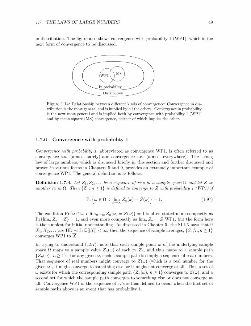
1.7. THE LAWS OF LARGE NUMBERS 49
in distribution. The figure also shows convergence with probability 1 (WP1), which is thenext form of convergence to be discussed.
"!# "!#
Distribution
In probability
WP1MS
Figure 1.14: Relationship between di↵erent kinds of convergence: Convergence in dis-tribution is the most general and is implied by all the others. Convergence in probabilityis the next most general and is implied both by convergence with probability 1 (WP1)and by mean square (MS) convergence, neither of which implies the other.
1.7.6 Convergence with probability 1
Convergence with probability 1, abbreviated as convergence WP1, is often referred to asconvergence a.s. (almost surely) and convergence a.e. (almost everywhere). The stronglaw of large numbers, which is discussed briefly in this section and further discussed andproven in various forms in Chapters 5 and 9, provides an extremely important example ofconvergence WP1. The general definition is as follows:
Definition 1.7.4. Let Z1, Z2, . . . be a sequence of rv’s in a sample space ⌦ and let Z beanother rv in ⌦. Then {Zn; n � 1} is defined to converge to Z with probability 1 (WP1) if
Prn! 2 ⌦ : lim
n!1Zn(!) = Z(!)
o= 1. (1.97)
The condition Pr{! 2 ⌦ : limn!1 Zn(!) = Z(!)} = 1 is often stated more compactly asPr{limn Zn = Z} = 1, and even more compactly as limn Zn = Z WP1, but the form hereis the simplest for initial understanding. As discussed in Chapter 5. the SLLN says that ifX1,X2, . . . are IID with E [|X|] < 1, then the sequence of sample averages, {Sn/n;n � 1}converges WP1 to X.
In trying to understand (1.97), note that each sample point ! of the underlying samplespace ⌦ maps to a sample value Zn(!) of each rv Zn, and thus maps to a sample path{Zn(!); n � 1}. For any given !, such a sample path is simply a sequence of real numbers.That sequence of real numbers might converge to Z(!) (which is a real number for thegiven !), it might converge to something else, or it might not converge at all. Thus a set of! exists for which the corresponding sample path {Zn(!); n � 1} converges to Z(!), and asecond set for which the sample path converges to something else or does not converge atall. Convergence WP1 of the sequence of rv’s is thus defined to occur when the first set ofsample paths above is an event that has probability 1.

50 CHAPTER 1. INTRODUCTION AND REVIEW OF PROBABILITY
For each !, the sequence {Zn(!); n � 1} is simply a sequence of real numbers, so we brieflyreview what the limit of such a sequence is. A sequence of real numbers b1, b2, . . . is said tohave a limit b if, for every ✏ > 0, there is an integer m✏ such that |bn� b| ✏ for all n � m✏.An equivalent statement is that b1, b2, . . . has a limit b if, for every integer k � 1, there isan integer m(k) such that |bn � b| 1/k for all n � m(k).
Figure 1.15 illustrates this definition for those, like the author, whose eyes blur on thesecond or third ‘there exists’, ‘such that’, etc. in a statement. As illustrated, an importantaspect of convergence of a sequence {bn; n � 1} of real numbers is that bn becomes close tob for large n and stays close for all su�ciently large values of n.
b1
b2
b3
b4
b5
b6
b7
m(1)m(2) m(3)
m(4)
b + 1
b + 1/2b + 1/3
b� 1/3b� 1/2
b� 1
b
Figure 1.15: Illustration of a sequence of real numbers b1, b2, . . . that converge to anumber b. The figure illustrates an integer m(1) such that for all n � m(1), bn lies inthe interval b ± 1. Similarly, for each k � 1, there is an integer m(k) such that bn liesin b ± 1/k for all n � m(k). Thus limn!1 bn = b means that for a sequence of evertighter constraints, the kth constraint can be met for all su�ciently large n, (i.e., alln � m(k)). Intuitively, convergence means that the elements b1, b2, . . . get close to band stay close. The sequence of positive integers m(1),m(2), . . . is non-decreasing, butotherwise arbitrary, depending only on the sequence {bn; n � 1}. For sequences thatconverge very slowly, the integers m(1),m(2), . . . are simply correspondingly larger.
Figure 1.16 gives an example of a sequence of real numbers that does not converge. Intu-itively, this sequence is close to 0 (and in fact identically equal to 0) for most large n, butit doesn’t stay close, because of ever more rare outages.
q q q q q q q q q q q q q q q q q q q q q q q q q qb1 b5 b25
0
3/4
Figure 1.16: Illustration of a non-convergent sequence of real numbers b1, b2, . . . . Thesequence is defined by bn = 3/4 for n = 1, 5, 25, . . . , 5j , . . . for all integer j � 0. For allother n, bn = 0. The terms for which bn 6= 0 become increasingly rare as n !1. Notethat bn 2 [�1, 1] for all n, but there is no m(2) such that bn 2 [�1
2 , 12 ] for all n � m(2).
Thus the sequence does not converge.
The following example illustrates how a sequence of rv’s can converge in probability but

1.8. RELATION OF PROBABILITY MODELS TO THE REAL WORLD 51
not converge WP1. The example also provides some clues as to why convergence WP1 isimportant.
Example 1.7.1. Consider a sequence {Yn; n � 1} of rv’s for which the sample pathsconstitute the following slight variation of the sequence of real numbers in Figure 1.16.In particular, as illustrated in Figure 1.17, the non-zero term at n = 5j in Figure 1.16 isreplaced by a non-zero term at a randomly chosen n in the interval34 [5j , 5j+1).
q q q q q q q q q q q q q q q q q q q q q q q q q q q q q q q q q q qq q q q q q q q q q q q q q q q q q q q q q q1 5 25
0
3/4
Figure 1.17: Illustration of a sample path of a sequence of rv’s {Yn;n � 0} where, foreach j � 0, Yn = 1 for an equiprobable choice of n 2 [5j , 5j+1) and Yn = 0 otherwise.
Since each sample path contains a single one in each segment [5j , 5j+1), and contains zeroeselsewhere, none of the sample paths converge. In other words, Pr{! : limYn(!) = 0} = 0.On the other hand Pr{Yn = 0} = 1� 5�j for 5j n < 5j+1, so limn!1 Pr{Yn = 0} = 1.
Thus this sequence of rv’s converges to 0 in probability, but does not converge to 0 WP1.This sequence also converges in mean square and (since it converges in probability) indistribution. Thus we have shown (by example) that convergence WP1 is not implied byany of the other types of convergence we have discussed. We will show in Section 5.2 thatconvergence WP1 does imply convergence in probability and in distribution but not in meansquare (as illustrated in Figure 1.14).
The interesting point in this example is that this sequence of rv’s is not bizarre (although itis somewhat specialized to make the analysis simple). Another important point is that thisdefinition of convergence has a long history of being accepted as the ‘useful,’ ‘natural,’ and‘correct’ way to define convergence for a sequence of real numbers. Thus it is not surprisingthat convergence WP1 will turn out to be similarly useful for sequences of rv’s.
There is a price to be paid in using the concept of convergence WP1. We must then lookat the entire sequence of rv’s and can no longer analyze finite n-tuples and then go to thelimit as n ! 1. This requires a significant additional layer of abstraction, which involvesadditional mathematical precision and initial loss of intuition. For this reason we put o↵further discussion of convergence WP1 and the SLLN until Chapter 5 where it is needed.
1.8 Relation of probability models to the real world
Whenever experienced and competent engineers or scientists construct a probability modelto represent aspects of some system that either exists or is being designed for some applica-tion, they must acquire a deep knowledge of the system and its surrounding circumstances,
34There is no special significance to the number 5 here other than making the figure easy to visualize. Wecould replace 5 by 2 or 3 etc.

52 CHAPTER 1. INTRODUCTION AND REVIEW OF PROBABILITY
and concurrently consider various types of probability models used in probabilistic analysesof the same or similar systems. Usually very simple probability models help in understandingthe real-world system, and knowledge about the real-world system helps in understandingwhat aspects of the system are well-modeled by a given probability model. For a text suchas this, there is insu�cient space to understand the real-world aspects of each system thatmight be of interest. We must use the language of various canonical real-world systems formotivation and insight when studying probability models for various classes of systems, butsuch models must necessarily be chosen more for their tutorial than practical value.
There is a danger, then, that readers will come away with the impression that analysis ismore challenging and important than modeling. To the contrary, for work on real-worldsystems, modeling is almost always more di�cult, more challenging, and more importantthan analysis. The objective here is to provide the necessary knowledge and insight aboutprobabilistic models so that the reader can later combine this with a deep understandingof particular real application areas. This will result in a useful interactive use of models,analysis, and experimentation.
In this section, our purpose is not to learn how to model real-world problems, since, assaid above, this requires deep and specialized knowledge of whatever application area is ofinterest. Rather it is to understand the following conceptual problem that was posed inSection 1.1. Suppose we have a probability model of some real-world experiment involvingrandomness in the sense expressed there. When the real-world experiment being modeled isperformed, there is an outcome, which presumably is one of the outcomes of the probabilitymodel, but there is no observable probability.
It appears to be intuitively natural, for experiments that can be carried out repeatedlyunder essentially the same conditions, to associate the probability of a given event withthe relative frequency of that event over many repetitions. We now have the backgroundto understand this approach. We first look at relative frequencies within the probabilitymodel, and then within the real world.
1.8.1 Relative frequencies in a probability model
We have seen that for any probability model, an extended probability model exists for nIID idealized experiments of the original model. For any event A in the original model,the indicator function IA is a random variable, and the relative frequency of A over n IIDexperiments is the sample average of n IID rv’s each with the distribution of IA. Fromthe weak law of large numbers, this relative frequency converges in probability to E [IA] =Pr{A}. By taking the limit n !1, the strong law of large numbers says that the relativefrequency of A converges with probability 1 to Pr{A}.
In plain English, this says that for large n, the relative frequency of an event (in the n-repetition IID model) is essentially the same as the probability of that event. The wordessentially is carrying a great deal of hidden baggage. For the weak law, for any ✏, � > 0,the relative frequency is within some ✏ of Pr{A} with a confidence level 1 � � whenevern is su�ciently large. For the strong law, the ✏ and � are avoided, but only by lookingdirectly at the limit n ! 1. Despite the hidden baggage, though, relative frequency and

1.8. RELATION OF PROBABILITY MODELS TO THE REAL WORLD 53
probability are related as indicated.
1.8.2 Relative frequencies in the real world
In trying to sort out if and when the laws of large numbers have much to do with real-worldexperiments, we should ignore the mathematical details for the moment and agree that forlarge n, the relative frequency of an event A over n IID trials of an idealized experimentis essentially Pr{A}. We can certainly visualize a real-world experiment that has the sameset of possible outcomes as the idealized experiment and we can visualize evaluating therelative frequency of A over n repetitions with large n. If that real-world relative frequencyis essentially equal to Pr{A}, and this is true for the various events A of greatest interest,then it is reasonable to hypothesize that the idealized experiment is a reasonable model forthe real-world experiment, at least so far as those given events of interest are concerned.
One problem with this comparison of relative frequencies is that we have carefully specifieda model for n IID repetitions of the idealized experiment, but have said nothing about howthe real-world experiments are repeated. The IID idealized experiments specify that theconditional probability of A at one trial is the same no matter what the results of the othertrials are. Intuitively, we would then try to isolate the n real-world trials so they don’t a↵ecteach other, but this is a little vague. The following examples help explain this problem andseveral others in comparing idealized and real-world relative frequencies.
Example 1.8.1. Coin tossing: Tossing coins is widely used as a way to choose the firstplayer in various games, and is also sometimes used as a primitive form of gambling. Itsimportance, however, and the reason for its frequent use, is its simplicity. When tossinga coin, we would argue from the symmetry between the two sides of the coin that eachshould be equally probable (since any procedure for evaluating the probability of one sideshould apply equally to the other). Thus since H and T are the only outcomes (the remotepossibility of the coin balancing on its edge is omitted from the model), the reasonable anduniversally accepted model for coin tossing is that H and T each have probability 1/2.
On the other hand, the two sides of a coin are embossed in di↵erent ways, so that the massis not uniformly distributed. Also the two sides do not behave in quite the same way whenbouncing o↵ a surface. Each denomination of each currency behaves slightly di↵erently inthis respect. Thus, not only do coins violate symmetry in small ways, but di↵erent coinsviolate it in di↵erent ways.
How do we test whether this e↵ect is significant? If we assume for the moment that succes-sive tosses of the coin are well-modeled by the idealized experiment of n IID trials, we canessentially find the probability of H for a particular coin as the relative frequency of H in asu�ciently large number of independent tosses of that coin. This gives us slightly di↵erentrelative frequencies for di↵erent coins, and thus slightly di↵erent probability models fordi↵erent coins.
The assumption of independent tosses is also questionable. Consider building a carefully en-gineered machine for tossing coins and using it in a vibration-free environment. A standardcoin is inserted into the machine in the same way for each toss and we count the numberof heads and tails. Since the machine has essentially eliminated the randomness, we would

54 CHAPTER 1. INTRODUCTION AND REVIEW OF PROBABILITY
expect all the coins, or almost all the coins, to come up the same way — the more precisethe machine, the less independent the results. By inserting the original coin in a randomway, a single trial might have equiprobable results, but successive tosses are certainly notindependent. The successive trials would be closer to independent if the tosses were doneby a slightly inebriated individual who tossed the coins high in the air.
The point of this example is that there are many di↵erent coins and many ways of tossingthem, and the idea that one model fits all is reasonable under some conditions and notunder others. Rather than retreating into the comfortable world of theory, however, notethat we can now find the relative frequency of heads for any given coin and essentially forany given way of tossing that coin.35
Example 1.8.2. Binary data: Consider the binary data transmitted over a communica-tion link or stored in a data facility. The data is often a mixture of encoded voice, video,graphics, text, etc., with relatively long runs of each, interspersed with various protocolsfor retrieving the original non-binary data.
The simplest (and most common) model for this is to assume that each binary digit is 0 or1 with equal probability and that successive digits are statistically independent. This is thesame as the model for coin tossing after the trivial modification of converting {H,T} into{0, 1}. This is also a rather appropriate model for designing a communication or storagefacility, since all n-tuples are then equiprobable (in the model) for each n, and thus thefacilities need not rely on any special characteristics of the data. On the other hand, if onewants to compress the data, reducing the required number of transmitted or stored bits perincoming bit, then a more elaborate model is needed.
Developing such an improved model would require finding out more about where the datais coming from — a naive application of calculating relative frequencies of n-tuples wouldprobably not be the best choice. On the other hand, there are well-known data compressionschemes that in essence track dependencies in the data and use them for compression in acoordinated way. These schemes are called universal data-compression schemes since theydon’t rely on a probability model. At the same time, they are best analyzed by looking athow they perform for various idealized probability models.
The point of this example is that choosing probability models often depends heavily on howthe model is to be used. Models more complex than IID binary digits are usually based onwhat is known about the input processes. Measuring relative frequencies and associatingthem with probabilities is the basic underlying conceptual connection between real-worldand models, but in practice this is essentially the relationship of last resort. For most ofthe applications we will consider, there is a long history of modeling to build on, withexperiments as needed.
Example 1.8.3. Fable: In the year 2008, the financial structure of the USA failed andthe world economy was brought to its knees. Much has been written about the role of greed
35We are not suggesting that distinguishing di↵erent coins for the sake of coin tossing is an importantproblem. Rather, we are illustrating that even in such a simple situation, the assumption of identicallyprepared experiments is questionable and the assumption of independent experiments is questionable. Theextension to n repetitions of IID experiments is not necessarily a good model for coin tossing. In otherwords, one has to question not only the original model but also the n-repetition model.

1.8. RELATION OF PROBABILITY MODELS TO THE REAL WORLD 55
on Wall Street and incompetence in Washington. Another aspect of the collapse, however,was a widespread faith in stochastic models for limiting risk. These models encouragedpeople to engage in investments that turned out to be far riskier than the models predicted.These models were created by some of the brightest PhD’s from the best universities, butthey failed miserably because they modeled everyday events very well, but modeled the rareevents and the interconnection of events poorly. They failed badly by not understandingtheir application, and in particular, by trying to extrapolate typical behavior when theirprimary goal was to protect against highly atypical situations. The moral of the fable isthat brilliant analysis is not helpful when the modeling is poor; as computer engineers say,“garbage in, garbage out.”
The examples above show that the problems of modeling a real-world experiment are oftenconnected with the question of creating a model for a set of experiments that are notexactly the same and do not necessarily correspond to the notion of independent repetitionswithin the model. In other words, the question is not only whether the probability model isreasonable for a single experiment, but also whether the IID repetition model is appropriatefor multiple copies of the real-world experiment.
At least we have seen, however, that if a real-world experiment can be performed many timeswith a physical isolation between performances that is well modeled by the IID repetitionmodel, then the relative frequencies of events in the real-world experiment correspond torelative frequencies in the idealized IID repetition model, which correspond to probabilitiesin the original model. In other words, under appropriate circumstances, the probabilitiesin a model become essentially observable over many repetitions.
We will see later that our emphasis on IID repetitions was done for simplicity. There areother models for repetitions of a basic model, such as Markov models, that we study later.These will also lead to relative frequencies approaching probabilities within the repetitionmodel. Thus, for repeated real-world experiments that are well modeled by these repetitionmodels, the real world relative frequencies approximate the probabilities in the model.
1.8.3 Statistical independence of real-world experiments
We have been discussing the use of relative frequencies of an event A in a repeated real-world experiment to test Pr{A} in a probability model of that experiment. This can bedone essentially successfully if the repeated trials correpond to IID trials in the idealizedexperiment. However, the statement about IID trials in the idealized experiment is a state-ment about probabilities in the extended n-trial model. Thus, just as we tested Pr{A} byrepeated real-world trials of a single experiment, we should be able to test Pr{A1, . . . , An}in the n-repetition model by a much larger number of real-world repetitions of n-tuplesrather than single trials.
To be more specific, choose two large integers, m and n, and perform the underlying real-world experiment mn times. Partition the mn trials into m runs of n trials each. For anygiven n-tuple A1, . . . , An of successive events, find the relative frequency (over m trials ofn tuples) of the n-tuple event A1, . . . , An. This can then be used essentially to test the

56 CHAPTER 1. INTRODUCTION AND REVIEW OF PROBABILITY
probability Pr{A1, . . . , An} in the model for n IID trials. The individual event probabilitiescan also be tested, so the condition for independence can be tested.
The observant reader will note that there is a tacit assumption above that successive ntuples can be modeled as independent, so it seems that we are simply replacing a bigproblem with a bigger problem. This is not quite true, since if the trials are dependentwith some given probability model for dependent trials, then this test for independence willessentially reject the independence hypothesis for large enough n. In other words, we cannot completely verify the correctness of an independence hypothesis for the n-trial model,although in principle we could eventually falsify it if it is false.
Choosing models for real-world experiments is primarily a subject for statistics, and we willnot pursue it further except for brief discussions when treating particular application areas.The purpose here has been to treat a fundamental issue in probability theory. As statedbefore, probabilities are non-observables — they exist in the theory but are not directlymeasurable in real-world experiments. We have shown that probabilities essentially becomeobservable in the real-world via relative frequencies over repeated trials.
1.8.4 Limitations of relative frequencies
Most real-world applications that are modeled by probability models have such a largesample space that it is impractical to conduct enough trials to choose probabilities fromrelative frequencies. Even a shu✏ed deck of 52 cards would require many more than 52! ⇡8⇥ 1067 trials for most of the outcomes to appear even once. Thus relative frequencies canbe used to test the probability of given individual events of importance, but are usuallyimpractical for choosing the entire model and even more impractical for choosing a modelfor repeated trials.
Since relative frequencies give us a concrete interpretation of what probability means, how-ever, we can now rely on other approaches, such as symmetry, for modeling. From sym-metry, for example, it is clear that all 52! possible arrangements of a card deck should beequiprobable after shu✏ing. This leads, for example, to the ability to calculate probabilitiesof di↵erent poker hands, etc., which are such popular exercises in elementary probabilityclasses.
Another valuable modeling procedure is that of constructing a probability model where thepossible outcomes are independently chosen n-tuples of outcomes in a simpler model. Moregenerally, most of the random processes to be studied in this text are defined as variousways of combining simpler idealized experiments.
What is really happening as we look at modeling increasingly sophisticated systems andstudying increasingly sophisticated models is that we are developing mathematical resultsfor simple idealized models and relating those results to real-world results (such as relatingidealized statistically independent trials to real-world independent trials). The associationof relative frequencies to probabilities forms the basis for this, but is usually exercised onlyin the simplest cases.
The way one selects probability models of real-world experiments in practice is to use

1.9. SUMMARY 57
scientific knowledge and experience, plus simple experiments, to choose a reasonable model.The results from the model (such as the law of large numbers) are then used both tohypothesize results about the real-world experiment and to provisionally reject the modelwhen further experiments show it to be highly questionable. Although the results aboutthe model are mathematically precise, the corresponding results about the real-world areat best insightful hypotheses whose most important aspects must be validated in practice.
1.8.5 Subjective probability
There are many useful applications of probability theory to situations other than repeatedtrials of a given experiment. When designing a new system in which randomness (of the typeused in probability models) is hypothesized, one would like to analyze the system beforeactually building it. In such cases, the real-world system does not exist, so indirect meansmust be used to construct a probability model. Often some sources of randomness, such asnoise, can be modeled in the absence of the system. Often similar systems or simulationcan be used to help understand the system and help in formulating appropriate probabilitymodels. However, the choice of probabilities is to a certain extent subjective.
Another type of situation (such as risk analysis for nuclear reactors) deals with a largenumber of very unlikely outcomes, each catastrophic in nature. Experimentation clearlycannot be used to establish probabilities, and it is not clear that probabilities have any realmeaning here. It can be helpful, however, to choose a probability model on the basis ofsubjective beliefs which can be used as a basis for reasoning about the problem.
Choosing a probability model on the basis of subjective beliefs can be helpful here if usedas a basis for reasoning about the problem. When handled well, this can at least make thesubjective biases clear, leading to a more rational approach. When handled poorly (as forexample in some risk analyses of large financial systems) it can hide both the real risks andthe arbitrary nature of possibly poor decisions.
We will not discuss the various, often ingenious, methods for choosing subjective proba-bilities. The reason is that subjective beliefs should be based on intensive and long termexposure to the particular problem involved; discussing these problems in abstract proba-bility terms weakens this link. We will focus instead on the analysis of idealized models.These can be used to provide insights for subjective models, and more refined and preciseresults for objective models.
1.9 Summary
This chapter started with an introduction into the correspondence between probability the-ory and real-world experiments involving randomness. While almost all work in probabilitytheory works with established probability models, it is important to think through whatthese probabilities mean in the real world, and elementary subjects rarely address thesequestions seriously.
The next section discussed the axioms of probability theory, along with some insights about

58 CHAPTER 1. INTRODUCTION AND REVIEW OF PROBABILITY
why these particular axioms were chosen. This was followed by a review of conditionalprobabilities, statistical independence, and random variables. Stochastic processes in theguise of the Bernoulli process was then introduced with an emphasis on asymptotic behavior.The review of probability was then resumed with an emphasis on the underlying structureof the field rather than reviewing details and problem solving techniques.
Next the laws of large numbers were developed and discussed at a somewhat deeper levelthan most elementary courses. This involved a fair amount of abstraction, combined withmathematical analysis. The central idea is that the sample average of n IID rv’s ap-proaches the mean with increasing n. As a special case, the relative frequency of an eventA approaches Pr{A}. What the word approaches means here is both tricky and vital inunderstanding probability theory. The strong law of large numbers and convergence WP1requires mathematical maturity, and was postponed to Chapter 5 where it is first used.
The final section came back to the fundamental problem of understanding the relationbetween probability theory and randomness in the real-world. It was shown, via the lawsof large numbers, that probabilities become essentially observable via relative frequenciescalculated over repeated experiments.
There are too many texts on elementary probability to mention here, and most of themserve to give added understanding and background to the material in this chapter. Werecommend Bertsekas and Tsitsiklis [2], both for a careful statement of the fundamentalsand for a wealth of well-chosen and carefully explained examples.
Texts that cover similar material to that here are [22] and [14]. Kolmogorov [17] is readablefor the mathematically mature and is also of historical interest as the translation of the 1933book that first put probability on a firm mathematical basis. Feller [8] is the classic extendedand elegant treatment of elementary material from a mature point of view. Rudin [23] isan excellent text on measure theory for those with advanced mathematical preparation.

1.10. EXERCISES 59
1.10 Exercises
Exercise 1.1. Let A1 and A2 be arbitrary events and show that Pr{A1S
A2}+Pr{A1A2} =Pr{A1} + Pr{A2}. Explain which parts of the sample space are being double counted onboth sides of this equation and which parts are being counted once.
Exercise 1.2. This exercise derives the probability of an arbitrary (non-disjoint) union ofevents, derives the union bound, and derives some useful limit expressions.
a) For 2 arbitrary events A1 and A2, show that
A1
[A2 = A1
[(A2�A1) where A2�A1 = A2A
c1.
Show that A1 and A2 � A1 are disjoint Hint: This is what Venn diagrams were inventedfor.
b) For an arbitrary sequence of events, {An; n � 1}, let B1 = A1 and for each n � 2 defineBn = An �
Sn�1m=1 Am. Show that B1, B2, . . . , are disjoint events and show that for each
n � 2,Sn
m=1 Am =Sn
m=1 Bm. Hint: Use induction.
c) Show that
Prn[1
n=1An
o= Pr
n[1
n=1Bn
o=
X1
n=1Pr{Bn} .
Hint: Use the axioms of probability for the second equality.
d) Show that for each n, Pr{Bn} Pr{An}. Use this to show that
Prn[1
n=1An
o
X1
n=1Pr{An} .
e) Show that Pr{S1
n=1 An} = limm!1 Pr{Sm
n=1 An}. Hint: Combine parts c) and b). Notethat this says that the probability of a limit of unions is equal to the limit of the probabilities.This might well appear to be obvious without a proof, but you will see situations later wheresimilar appearing interchanges cannot be made.
f) Show that Pr{T1
n=1 An} = limn!1 Pr{Tn
i=1 Ai}. Hint: Remember De Morgan’s equali-ties.
Exercise 1.3. Find the probability that a five card poker hand, chosen randomly from a52 card deck, contains 4 aces. That is, if all 52! arrangements of a deck of cards are equallylikely, what is the probability that all 4 aces are in the first 5 cards of the deck.
Exercise 1.4. Consider a sample space of 8 equiprobable sample points and let A1, A2, A3
be three events each of probability 1/2 such that Pr{A1A2A3} = Pr{A1}Pr{A2}Pr{A3}.
a) Create an example where Pr{A1A2} = Pr{A1A3} = 14 but Pr{A2A3} = 1
8 . Hint: Makea table with a row for each sample point and a column for each of the above 3 events andtry di↵erent ways of assigning sample points to events (the answer is not unique).

60 CHAPTER 1. INTRODUCTION AND REVIEW OF PROBABILITY
b) Show that, for your example, A2 and A3 are not independent. Note that the definitionof statistical independence would be very strange if it allowed A1, A2, A3 to be independentwhile A2 and A3 are dependent. This illustrates why the definition of independence requires(1.14) rather than just (1.15).
Exercise 1.5. This exercise shows that for all rv’s X, FX(x) is continuous from the right.
a) For any given rv X, any real number x, and each integer n � 1, let An = {! : X >x + 1/n}, and show that A1 ✓ A2 ✓ · · · . Use this and the corollaries to the axioms ofprobability to show that Pr
nSn�1 An
o= limn!1 Pr{An}.
b) Show that PrnS
n�1 An
o= Pr{X > x} and that Pr{X > x} = limn!1 Pr{X > x + 1/n}.
c) Show that for ✏ > 0, lim✏!0 Pr{X x + ✏} = Pr{X x}.
d) Define eFX(x) = Pr{X < x}. Show that eFX(x) is continuous from the left. In otherwords, the continuity from the right for the CDF arises from the almost arbitrary (butuniversally accepted) choice in defining the CDF as Pr{X x} rather than Pr{X < x}.
Exercise 1.6. Show that for a continuous nonnegative rv X,Z 1
0Pr{X > x} dx =
Z 1
0xfX(x) dx (1.98)
Hint 1: First rewrite Pr{X > x} on the left side of (1.98) asR1x fX(y) dy. Then think
through, to your level of comfort, how and why the order of integration can be interchngedin the resulting expression.
Hint 2: As an alternate approach, derive (1.98) using integration by parts.
Exercise 1.7. Suppose X and Y are discrete rv’s with the PMF pXY (xi, yj). Show (apicture will help) that this is related to the joint CDF by
pXY (xi, yj) = lim�>0,�!0
[F(xi, yj)� F(xi � �, yj)� F(xi, yj � �) + F(xi � �, yj � �)] .
Exercise 1.8. A variation of Example 1.5.1 is to let M be a random variable that takeson both positive and negative values with the PMF
pM (m) =1
2|m| (|m| + 1).
In other words, M is symmetric around 0 and |M | has the same PMF as the nonnegativerv N of Example 1.5.1.
a) Show thatP
m�0 mpM (m) = 1 andP
m<0 mpM (m) = �1. (Thus show that theexpectation of M not only does not exist but is undefined even in the extended real numbersystem.)

1.10. EXERCISES 61
b) Suppose that the terms inP1
m=�1mpM (m) are summed in the order of 2 positive termsfor each negative term (i.e., in the order 1, 2,�1, 3, 4,�2, 5, · · · ). Find the limiting value ofthe partial sums in this series. Hint: You may find it helpful to know that
limn!1
Xn
i=1
1i�Z n
1
1x
dx
�= �,
where � is the Euler-Mascheroni constant, � = 0.57721 · · · .
c) Repeat (b) where, for any given integer k > 0, the order of summation is k positive termsfor each negative term.
Exercise 1.9. (Proof of Theorem 1.4.1) The bounds on the binomial in this theorem arebased on the Stirling bounds. These say that for all n � 1, n! is upper and lower boundedby
p2⇡n
⇣n
e
⌘n< n! <
p2⇡n
⇣n
e
⌘ne1/12n. (1.99)
The ratiop
2⇡n(n/e)n/n! of the first two terms is monotonically increasing with n towardthe limit 1, and the ratio
p2⇡n(n/e)n exp(1/12n)/n! is monotonically decreasing toward
1. The upper bound is more accurate, but the lower bound is simpler and known as theStirling approximation. See [8] for proofs and further discussion of the above facts.
a) Show from (1.99) and from the above monotone property that✓
n
k
◆<
rn
2⇡k(n� k)nn
kk(n�k)n�k.
Hint: First show that n!/k! <p
n/k nnk�ke�n+k for k < n.
b) Use the result of (a) to upper bound pSn(k) by
pSn(k) <
rn
2⇡k(n� k)pk(1� p)n�knn
kk(n�k)n�k.
Show that this is equivalent to the upper bound in Theorem 1.4.1.
c) Show that✓
n
k
◆>
rn
2⇡k(n� k)nn
kk(n�k)n�k
1� n
12k(n� k)
�.
d) Derive the lower bound in Theorem 1.4.1.
e) Show that D(p̃kp) = p̃ ln( p̃p) + (1� p̃) ln(1�p̃
1�p) is 0 at p̃ = p and nonnegative elsewhere.
Exercise 1.10. Let X be a ternary rv taking on the 3 values 0, 1, 2 with probabilitiesp0, p1, p2 respectively. Find the median of X for each of the cases below.

62 CHAPTER 1. INTRODUCTION AND REVIEW OF PROBABILITY
a) p0 = 0.2, p1 = 0.4, p2 = 0.4.
b) p0 = 0.2, p1 = 0.2, p2 = 0.6.
c) p0 = 0.2, p1 = 0.3, p2 = 0.5.
Note 1: The median is not unique in (c). Find the interval of values that are medians. Note2: Some people force the median to be distinct by defining it as the midpoint of the intervalsatisfying the definition given here.
d) Now suppose that X is nonnegative and continuous with the density fX(x) = 1 for0 x 0.5 and fX(x) = 0 for 0.5 < x 1. We know that fX(x) is positive for all x > 1,but it is otherwise unknown. Find the median or interval of medians.
The median is sometimes (incorrectly) defined as that ↵ for which Pr{X > ↵} = Pr{X < ↵}.Show that it is possible for no such ↵ to exist. Hint: Look at the examples above.
Exercise 1.11. a) For any given rv Y , express E [|Y |] in terms ofRy<0 FY (y) dy andR
y�0 FcY(y) dy. Hint: Review the argument in Figure 1.4.
b) For some given rv X with E [|X|] < 1, let Y = X � ↵. Using (a), show that
E [|X � ↵|] =Z ↵
�1FX(x) dx +
Z 1
↵Fc
X(x) dx.
c) Show that E [|X � ↵|] is minimized over ↵ by choosing ↵ to be a median of X. Hint:Both the easy way and the most instructive way to do this is to use a graphical argumentillustrating the above integrals. Be careful to show that when the median is an interval, allpoints in this interval achieve the minimum.
Exercise 1.12. Let X be a rv with CDF FX(x). Find the CDF of the following rv’s.
a) The maximum of n IID rv’s, each with CDF FX(x).
b) The minimum of n IID rv’s, each with CDF FX(x).
c) The di↵erence of the rv’s defined in a) and b); assume X has a density fX(x).
Exercise 1.13. Let X and Y be rv’s in some sample space ⌦ and let Z = X + Y , i.e., foreach ! 2 ⌦, Z(!) = X(!) + Y (!). The purpose of this exercise is to show that Z is a rv.This is a mathematical fine point that many readers may prefer to simply accept withoutproof.
a) Show that the set of ! for which Z(!) is infinite or undefined has probability 0.
b) We must show that {! 2 ⌦ : Z(!) ↵} is an event for each real ↵, and we start byapproximating that event. To show that Z = X + Y is a rv, we must show that for eachreal number ↵, the set {! 2 ⌦ : X(!) + Y (!) ↵} is an event. Let B(n, k) = {! : X(!) k/n}
T{Y (!) ↵ + (1�k)/n} Let D(n) =
Sk B(n, k) and show that D(n) is an event.
c) On a 2 dimensional sketch for a given ↵, show the values of X(!) and Y (!) for which! 2 D(n). Hint: This set of values should be bounded by a staircase function.

1.10. EXERCISES 63
d) Show that
{! : X(!) + Y (!) ↵} =\
n�1D(n). (1.100)
Explain why this shows that Z = X + Y is a rv.
e) Explain why this implies that if Y = X1 + X2 + · · ·+ Xn and if X1,X2, . . . ,Xn are rv’s,then Y is a rv. Hint: Only one or two lines of explanation are needed.
Exercise 1.14. a) Let X1,X2, . . . ,Xn be rv’s with expected values X1, . . . ,Xn. Showthat E [X1 + · · · + Xn] = X1 + · · ·+Xn. You may assume that the rv’s have a joint densityfunction, but do not assume that the rv’s are independent.
b) Now assume that X1, . . . ,Xn are statistically independent and show that the expectedvalue of the product is equal to the product of the expected values.
c) Again assuming that X1, . . . ,Xn are statistically independent, show that the varianceof the sum is equal to the sum of the variances.
Exercise 1.15. (Stieltjes integration) a) Let h(x) = u(x) and FX(x) = u(x) where u(x) isthe unit step, i.e., u(x) = 0 for �1 < x < 0 and u(x) = 1 for x � 0. Using the definition ofthe Stieltjes integral in Footnote 19, show that
R 1�1 h(x)dFX(x) does not exist. Hint: Look
at the term in the Riemann sum including x = 0 and look at the range of choices for h(x) inthat interval. Intuitively, it might help initially to view dFX(x) as a unit impulse at x = 0.
b) Let h(x) = u(x � a) and FX(x) = u(x � b) where a and b are in (�1, +1). Show thatR 1�1 h(x)dFX(x) exists if and only if a 6= b. Show that the integral has the value 1 for a < b
and the value 0 for a > b. Argue that this result is still valid in the limit of integration over(�1, 1).
c) Let X and Y be independent discrete rv’s, each with a finite set of possible values. Showthat
R1�1 FX(z � y)dFY (y), defined as a Stieltjes integral, is equal to the distribution of
Z = X + Y at each z other than the possible sample values of Z, and is undefined at eachsample value of Z. Hint: Express FX and FY as sums of unit steps. Note: This failure ofStieltjes integration is not a serious problem; FZ(z) is a step function, and the integral isundefined at its points of discontinuity. We automatically define FZ(z) at those step valuesso that FZ is a CDF (i.e., is continuous from the right). This problem does not arise ifeither X or Y is continuous.
Exercise 1.16. Let X1,X2, . . . ,Xn, . . . be a sequence of IID continuous rv’s with thecommon probability density function fX(x); note that Pr{X=↵} = 0 for all ↵ and thatPr{Xi=Xj} = 0 for all i 6= j. For n � 2, define Xn as a record-to-date of the sequence ifXn > Xi for all i < n.
a) Find the probability that X2 is a record-to-date. Use symmetry to obtain a numericalanswer without computation. A one or two line explanation should be adequate.
b) Find the probability that Xn is a record-to-date, as a function of n � 1. Again usesymmetry.

64 CHAPTER 1. INTRODUCTION AND REVIEW OF PROBABILITY
c) Find a simple expression for the expected number of records-to-date that occur overthe first m trials for any given integer m. Hint: Use indicator functions. Show that thisexpected number is infinite in the limit m !1.
Exercise 1.17. (Continuation of Exercise 1.16)
a) Let N1 be the index of the first record-to-date in the sequence. Find Pr{N1 > n} foreach n � 2. Hint: There is a far simpler way to do this than working from (b) in Exercise1.16.
b) Show that N1 is a rv.
c) Show that E [N1] = 1.
d) Let N2 be the index of the second record-to-date in the sequence. Show that N2 is a rv.Hint: You need not find the CDF of N2 here.
e) Contrast your result in (c) to the result from (c) of Exercise 1.16 saying that the expectednumber of records-to-date is infinite over an an infinite number of trials. Note: this shouldbe a shock to your intuition — there is an infinite expected wait for the first of an infinitesequence of occurrences, each of which must eventually occur.
Exercise 1.18. (Another direction from Exercise 1.16) a) For any given n � 2, find theprobability that Xn and Xn+1 are both records-to-date. Hint: The idea in (b) of 1.16 ishelpful here, but the result is not.
b) Is the event that Xn is a record-to-date statistically independent of the event that Xn+1
is a record-to-date?
c) Find the expected number of adjacent pairs of records-to-date over the sequence X1,X2, . . . .Hint: A helpful fact here is that 1
n(n+1) = 1n �
1n+1 .
Exercise 1.19. a) Assume that X is a nonnegative discrete rv taking on values a1, a2, . . . ,and let Y = h(X) for some nonnegative function h. Let bi = h(ai), i�1 be the ith valuetaken on by Y . Show that E [Y ] =
Pi bipY (bi) =
Pi h(ai)pX(ai). Find an example where
E [X] exists but E [Y ] = 1.
b) Let X be a nonnegative continuous rv with density fX(x) and let h(x) be di↵erentiable,nonnegative, and nondecreasing in x. Let A(�) =
Pn�1 h(n�)[F(n�)� F(n�� �)], i.e., A(�)
is a �th order approximation to the Stieltjes integralR
h(x)dF(x). Show that if A(1) < 1,then A(2�k) A(2�(k�1)) < 1 for k � 1. Show from this that
Rh(x) dF(x) converges to
a finite value. Note: this is a very special case, but it can be extended to many cases ofinterest. It seems better to consider these convergence questions as required rather thanconsider them in general.
Exercise 1.20. a) Consider a positive, integer-valued rv Y whose CDF is given at integervalues by
FY (y) = 1� 2(y + 1)(y + 2)
for integer y � 0.

1.10. EXERCISES 65
Use (1.31) to show that E [Y ] = 2. Hint: Note that 1/[(y+1)(y+2)] = 1/(y+1)�1/(y+2).
b) Find the PMF of Y and use it to check the value of E [Y ].
c) Let X be another positive, integer-valued rv. Assume its conditional PMF is given by
pX|Y (x|y) =1y
for 1 x y.
Find E [X | Y = y] and use it to show that E [X] = 3/2. Explore finding pX(x) until you areconvinced that using the conditional expectation to calculate E [X] is considerably easierthan using pX(x).
d) Let Z be another integer-valued rv with the conditional PMF
pZ|Y (z|y) =1y2
for 1 z y2.
Find E [Z | Y = y] for each integer y � 1 and find E [Z].
Exercise 1.21. a) Show that, for uncorrelated rv’s, the expected value of the product isequal to the product of the expected values (by definition, X and Y are uncorrelated ifE⇥(X �X)(Y � Y )
⇤= 0).
b) Show that if X and Y are uncorrelated, then the variance of X + Y is equal to thevariance of X plus the variance of Y .
c) Show that if X1, . . . ,Xn are uncorrelated, then the variance of the sum is equal to thesum of the variances.
d) Show that independent rv’s are uncorrelated.
e) Let X,Y be identically distributed ternary valued random variables with the PMFpX(�1) = pX(1) = 1/4; pX(0) = 1/2. Find a simple joint probability assignment suchthat X and Y are uncorrelated but dependent.
f) You have seen that the moment generating function of a sum of independent rv’s is equalto the product of the individual moment generating functions. Give an example where thisis false if the variables are uncorrelated but dependent.
Exercise 1.22. Suppose X has the Poisson PMF, pX(n) = �n exp(��)/n! for n � 0 andY has the Poisson PMF, pY (n) = µn exp(�µ)/n! for n � 0. Assume that X and Y areindependent. Find the distribution of Z = X + Y and find the conditional distribution ofY conditional on Z = n.
Exercise 1.23. a) Suppose X, Y and Z are binary rv’s, each taking on the value 0 withprobability 1/2 and the value 1 with probability 1/2. Find a simple example in whichX, Y , Z are statistically dependent but are pairwise statistically independent (i.e., X, Yare statistically independent, X, Z are statistically independent, and Y , Z are statistically

66 CHAPTER 1. INTRODUCTION AND REVIEW OF PROBABILITY
independent). Give pXY Z(x, y, z) for your example. Hint: In the simplest example, thereare four joint values for x, y, z that have probability 1/4 each.
b) Is pairwise statistical independence enough to ensure that
EhYn
i=1Xi
i=Yn
i=1E [Xi] .
for a set of rv’s X1, . . . ,Xn?
Exercise 1.24. Show that E [X] is the value of ↵ that minimizes E⇥(X � ↵)2
⇤.
Exercise 1.25. For each of the following random variables, find the endpoints r� and r+
of the interval for which the moment generating function g(r) exists. Determine in eachcase whether gX(r) exists at r� and r+. For parts a) and b) you should also find and sketchg(r). For parts c) and d), g(r) has no closed form.
a) Let �, ✓, be positive numbers and let X have the density
fX(x) =12� exp(��x); x � 0; fX(x) =
12✓ exp(✓x); x < 0.
b) Let Y be a Gaussian random variable with mean m and variance �2.
c) Let Z be a nonnegative random variable with density
fZ(z) = k(1 + z)�2 exp(��z); z � 0.
where � > 0 and k = [Rz�0(1 + z)�2 exp(��z)dz]�1. Hint: Do not try to evaluate gZ(r).
Instead, investigate values of r for which the integral is finite and infinite.
d) For the Z of (c), find the limit of �0(r) as r approaches � from below. Then replace(1 + z)2 with |1 + z|3 in the definition of fZ(z) and K and show whether the above limit isthen finite or not. Hint: no integration is required.
Exercise 1.26. a) Assume that the MGF of the random variable X exists (i.e., is finite)in the interval (r�, r+), r� < 0 < r+, and assume r� < r < r+ throughout. For any finiteconstant c, express the moment generating function of X � c, i.e., g(X�c)(r), in terms ofgX(r) and show that g(X�c)(r) exists for all r in (r�, r+). Explain why g00(X�c)(r) � 0.
b) Show that g00(X�c)(r) = [g00X(r)� 2cg0X(r) + c2gX(r)]e�rc.
c) Use a) and b) to show that g00X(r)gX(r)� [g0X(r)]2 � 0, Let �X(r) = ln gX(r) and showthat �00X(r) � 0. Hint: Choose c = g0X(r)/gX(r).
d) Assume that X is non-deterministic, i.e., that there is no value of ↵ such that Pr{X = ↵} =1. Show that the inequality sign “�” may be replaced by “>” everywhere in a), b) and c).

1.10. EXERCISES 67
Exercise 1.27. A computer system has n users, each with a unique name and password.Due to a software error, the n passwords are randomly permuted internally (i.e. each ofthe n! possible permutations are equally likely. Only those users lucky enough to have hadtheir passwords unchanged in the permutation are able to continue using the system.
a) What is the probability that a particular user, say user 1, is able to continue using thesystem?
b) What is the expected number of users able to continue using the system? Hint: Let Xi
be a rv with the value 1 if user i can use the system and 0 otherwise.
Exercise 1.28. Suppose the rv X is continuous and has the CDF FX(x). Consider anotherrv Y = FX(X). That is, for each sample point ! such that X(!) = x, we have Y (!) =FX(x). Show that Y is uniformly distributed in the interval 0 to 1.
Exercise 1.29. Let Z be an integer-valued rv with the PMF pZ(n) = 1/k for 0 n k�1.Find the mean, variance, and moment generating function of Z. Hint: An elegant way todo this is to let U be a uniformly distributed continuous rv over (0, 1] that is independentof Z. Then U + Z is uniform over (0, k]. Use the known results about U and U + Z to findthe mean, variance, and MGF for Z.
Exercise 1.30. (Alternate approach 1 to the Markov inequality) a) Let Y be a nonnegativerv and y > 0 be some fixed number. Let A be the event that Y � y. Show that y IA Y(i.e., that this inequality is satisfied for every ! 2 ⌦).
b) Use your result in (a) to prove the Markov inequality.
Exercise 1.31. (Alternate approach 2 to the Markov inequality) a) Minimize E [Y ] overall nonnegative rv’s such that Pr{Y � b} = � for some given b > 0 and 0 < � < 1. Hint:Use a graphical argument similar to that in Figure 1.7. What is the rv that achieves theminimum. Hint: It is binary.
b) Use (a) to prove the Markov inequality and also point out the distribution that meetsthe inequality with equality.
Exercise 1.32. (The one-sided Chebyshev inequality) This inequality states that if a zero-mean rv X has a variance �2, then it satisfies the inequality
Pr{X � b} �2
�2 + b2for every b > 0, (1.101)
with equality for some b only if X is binary and Pr{X = b} = �2/(�2 + b2). We prove thishere using the same approach as in Exercise 1.31. Let X be a zero-mean rv that satisfiesPr{X � b} = � for some b > 0 and 0 < � < 1. The variance �2 of X can be expressed as
�2 =Z b�
�1x2fX(x) dx +
Z 1
bx2 fX(x) dx (1.102)

68 CHAPTER 1. INTRODUCTION AND REVIEW OF PROBABILITY
We will first minimize �2 over all zero-mean X satisfying Pr{X � b} = �.
a) Show that the second integral in (1.102) satisfiesR1b x2fX(x) dx � b2�.
b) Show that the first integral in (1.102) is constrained byZ b�
�1fX(x) dx = 1� � and
Z b�
�1xfX(x) dx �b�.
c) Minimize the first integral in (1.102) subject to the constraints in (b). Hint: If you scalefX(x) up by 1/(1� �), it integrates to 1 over (�1, b) and the second constraint becomesan expectation. You can then minimize the first integral in (1.102) by inspection.
d) Combine the results in a) and c) to show that �2 � b2�/(1 � �). Find the minimizingdistribution. Hint: It is binary.
e) Use (d) to establish (1.101). Also show (trivially) that if Y has a mean Y and variance�2, then Pr
�Y � Y � b
�2/(�2 + b2)
Exercise 1.33. (Proof of (1.48)) Here we show that if X is a zero-mean rv with a variance�2, then the median ↵ satisfies |↵| �.
a) First show that |↵| � for the special case where X is binary with equiprobable valuesat ±�.
b) For all zero-mean rv’s X with variance �2 other than the special case in a), show that
Pr{X � �} < 0.5.
Hint: Use the one-sided Chebyshev inequality of Exercise 1.32.
c) Show that Pr{X � ↵} � 0.5. Other than the special case in a), show that this impliesthat ↵ < �.
d) Other than the special case in a), show that |↵| < �. Hint: repeat b) and c) for the rv�X. You have then shown that |↵| � with equality only for the binary case with values±�. For rv’s Y with a non-zero mean, this shows that |↵� Y | �.
Exercise 1.34. We stressed the importance of the mean of a rv X in terms of its associationwith the sample average via the WLLN. Here we show that there is a form of WLLN for themedian and for the entire CDF, say FX(x) of X via su�ciently many independent samplevalues of X.
a) For any given y, let Ij(y) be the indicator function of the event {Xj y} whereX1,X2, . . . ,Xj , . . . are IID rv’s with the CDF FX(x). State the WLLN for the IID rv’s{I1(y), I2(y), . . . }.
b) Does the answer to (a) require X to have a mean or variance?
c) Suggest a procedure for evaluating the median of X from the sample values of X1,X2, . . . .Assume that X is a continuous rv and that its PDF is positive in an open interval aroundthe median. You need not be precise, but try to think the issue through carefully.

1.10. EXERCISES 69
What you have seen here, without stating it precisely or proving it is that the median hasa law of large numbers associated with it, saying that the sample median of n IID samplesof a rv is close to the true median with high probability.
Exercise 1.35. a) Show that for any 0 < k < n✓
n
k + 1
◆✓
n
k
◆n� k
k.
b) Extend (a) to show that, for all ` n� k,✓
n
k + `
◆✓
n
k
◆n� k
k
�`
.
c) Let p̃ = k/n and q̃ = 1� p̃. Let Sn be the sum of n binary IID rv’s with pX(0) = q andpX(1) = p. Show that for all ` n� k,
pSn(k + `) pSn(k)✓
q̃p
p̃q
◆`
.
d) For k/n > p, show that Pr{Sn � k} p̃qp̃�p pSn(k).
e) Now let ` be fixed and k = dnp̃e for fixed p̃ such that 1 > p̃ > p. Argue that as n !1,
pSn(k + `) ⇠ pSn(k)✓
q̃p
p̃q
◆`
and Pr{Sn � k} ⇠ p̃q
p̃� ppSn(k),
where a(n) ⇠ b(n) means that limn!1 a(n)/b(n) = 1.
Exercise 1.36. A sequence {an; n � 1} of real numbers has the limit 0 if for all ✏ > 0,there is an m(✏) such that |an| ✏ for all n � m(✏). Show that the sequences in parts a)and b) below satisfy limn!1 an = 0 but the sequence in (c) does not have a limit.
a) an = 1ln(ln(n+1))
b) an = n10 exp(�n)
c) an = 1 for n = 10` for each positive integer ` and an = 0 otherwise.
d) Show that the definition can be changed (with no change in meaning) by replacing ✏with either 1/k or 2�k for every positive integer k.
Exercise 1.37. Represent the MGF of a rv X by
gX(r) =Z 0
�1erxdF(x) +
Z 1
0erxdF(x).
In each of the following parts, you are welcome to restrict X to be either discrete or con-tinuous.

70 CHAPTER 1. INTRODUCTION AND REVIEW OF PROBABILITY
a) Show that the first integral always exists (i.e., is finite) for r � 0 and that the secondintegral always exists for r 0.
b) Show that if the second integral exists for a given r1 > 0, then it also exists for all r inthe range 0 r r1.
c) Show that if the first integral exists for a given r2 < 0, then it also exists for all r in therange r2 r 0.
d) Show that the range of r over which gX(r) exists is an interval from some r� 0 tosome r+ � 0 (the interval might or might not include each endpoint, and either or both endpoint might be 0, 1, or any point between).
e) Find an example where r+ = 1 and the MGF does not exist for r = 1. Find anotherexample where r+ = 1 and the MGF does exist for r = 1. Hint: Consider fX(x) =e�x for x � 0 and figure out how to modify it to fY (y) so that
R10 eyfY (y) dy < 1 butR1
0 ey+✏yfY (y) = 1 for all ✏ > 0.
Exercise 1.38. Let {Xn; n � 1} be a sequence of independent but not identically dis-tributed rv’s. We say that the weak law of large numbers (WLLN) holds for this sequenceif for all ✏ > 0
limn!1
Pr⇢���Sn
n� E [Sn]
n
��� � ✏
�= 0 where Sn = X1 + X2 + · · · + Xn. (WL).
a) Show that the WLLN holds if there is some constant A such that �2Xn A for all n.
b) Suppose that �2Xn An1�↵ for some ↵ < 1 and for all n. Show that the WLLN holds
in this case.
Exercise 1.39. Let {Xi; i � 1} be IID binary rv’s. Let Pr{Xi = 1} = �, Pr{Xi = 0} =1 � �. Let Sn = X1 + · · · + Xn. Let m be an arbitrary but fixed positive integer. Think!then evaluate the following and explain your answers:
a) limn!1P
i:n��min�+m Pr{Sn = i}
b) limn!1P
i:0in�+m Pr{Sn = i}
c) limn!1P
i:n(��1/m)in(�+1/m) Pr{Sn = i}.
Exercise 1.40. The WLLN is said to hold for a zero-mean sequence {Sn; n � 1} if
limn!1
Pr⇢����Sn
n
���� > ✏
�= 0 for every ✏ > 0.
The CLT is said to hold for {Sn; n � 1} if for some � > 0 and all z 2 R,
limn!1
Pr⇢
Sn
�p
n z
�= �(z),

1.10. EXERCISES 71
where �(z) is the normal CDF. Show that if the CLT holds, then the WLLN holds also.Note 1: If you hate ✏, � arguments, you will hate this. Note 2: It will probably ease thepain if you convert the WLLN statement to: For every ✏ > 0, � > 0 there exists an n(✏, �)such that for every n � n(✏, �),
Pr⇢
Sn
n< �✏
� � and Pr
⇢Sn
n> 1� ✏
� �. (i)
Exercise 1.41. (Details in the proof of Theorem 1.7.4)
a) Show that if X1,X2, . . . are IID, then the truncated versions X̆1, X̆2, . . . are also IID.
b) Show that each X̆i has a finite mean EhX̆i
and finite variance �2X̆
. Show that the
variance is upper bounded by the second moment around the original mean X, i.e., showthat �2
X̆ E
h| X̆ � E [X] |2
i.
c) Assume that X̆i is Xi truncated to X ± b. Show that |X̆ �X| b and that |X̆ �X| |X �X|. Use this to show that �2
X̆ bE
⇥|X �X|
⇤ 2bE [|X|].
d) Let S̆n = X̆1 + · · · + X̆n and show that for any ✏ > 0,
Pr
(�����S̆n
n� E
hX̆i����� �
✏
2
) 8bE [|X|]
n✏2.
e) Use Figure 1.13, along with (1.34), to show that for all su�ciently large b,���E hX � X̆
i ��� ✏/2. Use this to show that
Pr
(�����S̆n
n� E [X]
����� � ✏
) 8bE [|X|]
n✏2for all large enough b.
f) Use the following equation to justify (1.96).
Pr⇢ ����Sn
n� E [X]
���� > ✏
�= Pr
⇢ ����Sn
n� E [X]
���� > ✏\
Sn = S̆n
�
+ Pr⇢ ����Sn
n� E [X]
���� > ✏\
Sn 6= S̆n
�.
Exercise 1.42. Let {Xi; i � 1} be IID rv’s with mean 0 and infinite variance. Assumethat E
⇥|Xi|1+h
⇤= � for some given h, 0 < h < 1 and some finite �. Let Sn = X1+ · · ·+Xn.
a) Show that Pr{|Xi| � y} � y�1�h
b) Let {X̆i; i � 1} be truncated variables X̆i =
8<:
b : Xi � bXi : �b Xi b�b : Xi �b

72 CHAPTER 1. INTRODUCTION AND REVIEW OF PROBABILITY
Show that EhX̆2
i 2�b1�h
1�h . Hint: For a nonnegative rv Z, E⇥X2
⇤=R10 2 z Pr{Z � z} dz
(you can establish this, if you wish, by integration by parts).
c) Let S̆n = X̆1 + . . . + X̆n. Show that PrnSn 6= S̆n
o n�b�1�h
d) Show that Pr���Sn
n
�� � ✏ �
h2b1�h
(1�h)n✏2 + nb1+h
i.
e) Optimize your bound with respect to b. How fast does this optimized bound approach0 with increasing n?
Exercise 1.43. (MS convergence =) convergence in probability) Assume that{Zn; n � 1} is a sequence of rv’s and ↵ is a number with the property that limn!1 E
⇥(Zn � ↵)2
⇤=
0.
a) Let ✏ > 0 be arbitrary and show that for each n � 0,
Pr{|Zn � ↵| � ✏} E⇥(Zn � ↵)2
⇤✏2
.
b) For the ✏ above, let � > 0 be arbitrary. Show that there is an integer m such thatE⇥(Zn � ↵)2
⇤ ✏2� for all n � m.
c) Show that this implies convergence in probability.
Exercise 1.44. Let X1,X2 . . . be a sequence of IID rv’s each with mean 0 and variance �2.Let Sn = X1 + · · · + Xn for all n and consider the random variable Sn/�
pn� S2n/�
p2n.
Find the limiting CDF for this sequence of rv0s as n !1. The point of this exercise is tosee clearly that the CDF of Sn/�
pn� S2n/�
p2n is converging in n but that the sequence
of rv’s is not converging in any reasonable sense.
Exercise 1.45. Verify (1.57), i.e., verify that limy!1 yPr{Y�y} = 0 if Y � 0 and Y < 1.Hint: Show that yPr{Y�y}
Rz�y zdFY (z) and show that limy!1
Rz�y zdFY (z) = 0.
Exercise 1.46. Show thatQ
m�n(1� 1/m) = 0. Hint: Show that✓
1� 1m
◆= exp
✓ln✓
1� 1m
◆◆ exp
✓� 1
m
◆.
Exercise 1.47. Consider a discrete rv X with the PMF
pX(�1) = (1� 10�10)/2,pX(1) = (1� 10�10)/2,
pX(1012) = 10�10.
a) Find the mean and variance of X. Assuming that {Xm; m � 1} is an IID sequence withthe distribution of X and that Sn = X1 + · · · + Xn for each n, find the mean and varianceof Sn. (no explanations needed.)

1.10. EXERCISES 73
b) Let n = 106 and describe the event {Sn 106} in words. Find an exact expression forPr�Sn 106
= FSn(106).
c) Find a way to use the union bound to get a simple upper bound and approximation of1� FSn(106).
d) Sketch the CDF of Sn for n = 106. You can choose the horizontal axis for your sketchto go from �1 to +1 or from �3 ⇥ 103 to 3 ⇥ 103 or from �106 to 106 or from 0 to 1012,whichever you think will best describe this CDF.
e) Now let n = 1010. Give an exact expression for Pr�Sn 1010
and show that this can
be approximated by e�1. Sketch the CDF of Sn for n = 1010, using a horizontal axis goingfrom slightly below 0 to slightly more than 2⇥ 1012. Hint: First view Sn as conditioned onan appropriate rv.
f) Can you make a qualitative statement about how the CDF of a rv X a↵ects the requiredsize of n before the WLLN and the CLT provide much of an indication about Sn.
Exercise 1.48. Let {Yn; n � 1} be a sequence of rv’s and assume that limn!1 E [|Yn|] = 0.Show that {Yn; n � 1} converges to 0 in probability. Hint 1: Look for the easy way. Hint2: The easy way uses the Markov inequality.