stochastic processes and applicationspavl/stoch_proc_notes-ch1-3.pdf · stochastic processes and...
TRANSCRIPT
STOCHASTIC PROCESSES ANDAPPLICATIONS
G.A. PavliotisDepartment of Mathematics
Imperial College London
February 2, 2014

2
Contents
1 Introduction 11.1 Historical Overview . . . . . . . . . . . . . . . . . . . . . . . . . 11.2 The One-Dimensional Random Walk . . . . . . . . . . . . . . . . 31.3 Why Randomness . . . . . . . . . . . . . . . . . . . . . . . . . . 61.4 Discussion and Bibliography . . . . . . . . . . . . . . . . . . . . 71.5 Exercises . . . . . . . . . . . . . . . . . . . . . . . . . . . . . . 7
2 Elements of Probability Theory 92.1 Basic Definitions from Probability Theory . . . . . . . . . . . .. 9
2.1.1 Conditional Probability . . . . . . . . . . . . . . . . . . . 112.2 Random Variables . . . . . . . . . . . . . . . . . . . . . . . . . . 12
2.2.1 Expectation of Random Variables . . . . . . . . . . . . . 162.3 Conditional Expecation . . . . . . . . . . . . . . . . . . . . . . . 182.4 The Characteristic Function . . . . . . . . . . . . . . . . . . . . . 182.5 Gaussian Random Variables . . . . . . . . . . . . . . . . . . . . 192.6 Types of Convergence and Limit Theorems . . . . . . . . . . . . 232.7 Discussion and Bibliography . . . . . . . . . . . . . . . . . . . . 252.8 Exercises . . . . . . . . . . . . . . . . . . . . . . . . . . . . . . 25
3 Basics of the Theory of Stochastic Processes 293.1 Definition of a Stochastic Process . . . . . . . . . . . . . . . . . 293.2 Stationary Processes . . . . . . . . . . . . . . . . . . . . . . . . 31
3.2.1 Strictly Stationary Processes . . . . . . . . . . . . . . . . 313.2.2 Second Order Stationary Processes . . . . . . . . . . . . 323.2.3 Ergodic Properties of Second-Order Stationary Processes . 37
3.3 Brownian Motion . . . . . . . . . . . . . . . . . . . . . . . . . . 393.4 Other Examples of Stochastic Processes . . . . . . . . . . . . . .44
i

ii CONTENTS
3.5 The Karhunen-Loeve Expansion . . . . . . . . . . . . . . . . . . 463.6 Discussion and Bibliography . . . . . . . . . . . . . . . . . . . . 513.7 Exercises . . . . . . . . . . . . . . . . . . . . . . . . . . . . . . 51
Chapter 1
Introduction
In this chapter we introduce some of the concepts and techniques that we will studyin this book. In Section 1.1 we present a brief historical overview on the develop-ment of the theory of stochastic processes in the twentieth century. In Section 1.2we introduce the one-dimensional random walk an we use this example in orderto introduce several concepts such Brownian motion, the Markov property. Somecomments on the role of probabilistic modeling in the physical sciences are of-fered in Section 1.3. Discussion and bibliographical comments are presented inSection 1.4. Exercises are included in Section 1.5.
1.1 Historical Overview
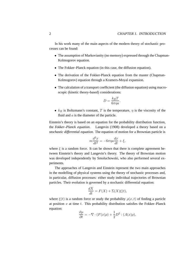
The theory of stochastic processes, at least in terms of its application to physics,started with Einstein’s work on the theory of Brownian motion: Concerning themotion, as required by the molecular-kinetic theory of heat, of particles suspendedin liquids at rest(1905) and in a series of additional papers that were published inthe period1905 − 1906. In these fundamental works, Einstein presented an expla-nation of Brown’s observation (1827) that when suspended inwater, small pollengrains are found to be in a very animated and irregular state of motion. In devel-oping his theory Einstein introduced several concepts thatstill play a fundamentalrole in the study of stochastic processes and that we will study in this book. Usingmodern terminology, Einstein introduced a Markov chain model for the motion ofthe particle (molecule, pollen grain...). Furthermore, heintroduced the idea that itmakes more sense to talk about the probability of finding the particle at positionxat timet, rather than about individual trajectories.
1
2 CHAPTER 1. INTRODUCTION
In his work many of the main aspects of the modern theory of stochastic pro-cesses can be found:
• The assumption of Markovianity (no memory) expressed through the Chapman-Kolmogorov equation.
• The Fokker–Planck equation (in this case, the diffusion equation).
• The derivation of the Fokker-Planck equation from the master (Chapman-Kolmogorov) equation through a Kramers-Moyal expansion.
• The calculation of a transport coefficient (the diffusion equation) using macro-scopic (kinetic theory-based) considerations:
D =kBT
6πηa.
• kB is Boltzmann’s constant,T is the temperature,η is the viscosity of thefluid anda is the diameter of the particle.
Einstein’s theory is based on an equation for the probability distribution function,the Fokker–Planck equation. Langevin (1908) developed a theory based on astochastic differential equation. The equation of motion for a Brownian particle is
md2x
dt2= −6πηa
dx
dt+ ξ,
whereξ is a random force. It can be shown that there is complete agreement be-tween Einstein’s theory and Langevin’s theory. The theory of Brownian motionwas developed independently by Smoluchowski, who also performed several ex-periments.
The approaches of Langevin and Einstein represent the two main approachesin the modelling of physical systems using the theory of stochastic processes and,in particular, diffusion processes: either study individual trajectories of Brownianparticles. Their evolution is governed by a stochastic differential equation:
dX
dt= F (X) + Σ(X)ξ(t),
whereξ(t) is a random force or study the probabilityρ(x, t) of finding a particleat positionx at time t. This probability distribution satisfies the Fokker–Planckequation:
∂ρ
∂t= −∇ · (F (x)ρ) +
1
2D2 : (A(x)ρ),
1.2. THE ONE-DIMENSIONAL RANDOM WALK 3
whereA(x) = Σ(x)Σ(x)T . The theory of stochastic processes was developedduring the20th century by several mathematicians and physicists including Smolu-chowksi, Planck, Kramers, Chandrasekhar, Wiener, Kolmogorov, Ito, Doob.
1.2 The One-Dimensional Random Walk
We let time be discrete, i.e.t = 0, 1, . . . . Consider the following stochasticprocessSn: S0 = 0; at each time step it moves to±1 with equal probability1
2 .
In other words, at each time step we flip a fair coin. If the outcome is heads,we move one unit to the right. If the outcome is tails, we move one unit to the left.
Alternatively, we can think of the random walk as a sum of independent randomvariables:
Sn =
n∑
j=1
Xj ,
whereXj ∈ −1, 1 with P(Xj = ±1) = 12 .
We can simulate the random walk on a computer:
• We need a (pseudo)random number generator to generaten independent ran-dom variables which are uniformly distributed in the interval [0,1].
• If the value of the random variable is> 12 then the particle moves to the left,
otherwise it moves to the right.
• We then take the sum of all these random moves.
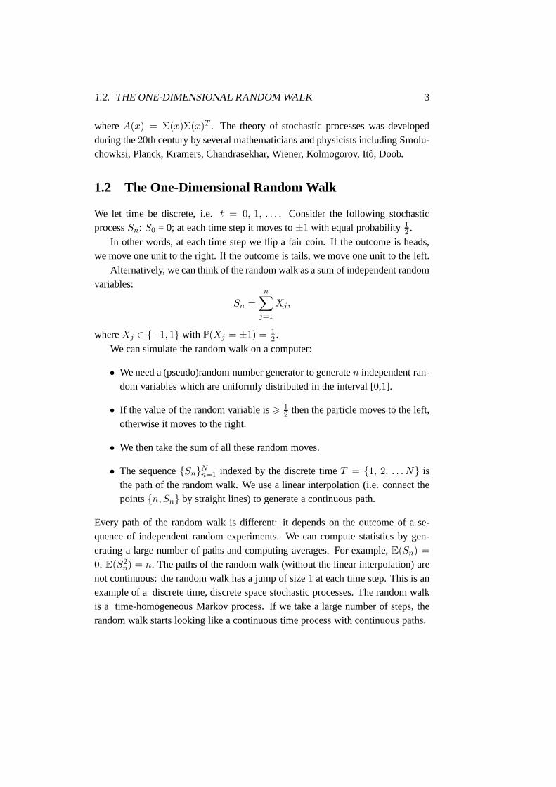
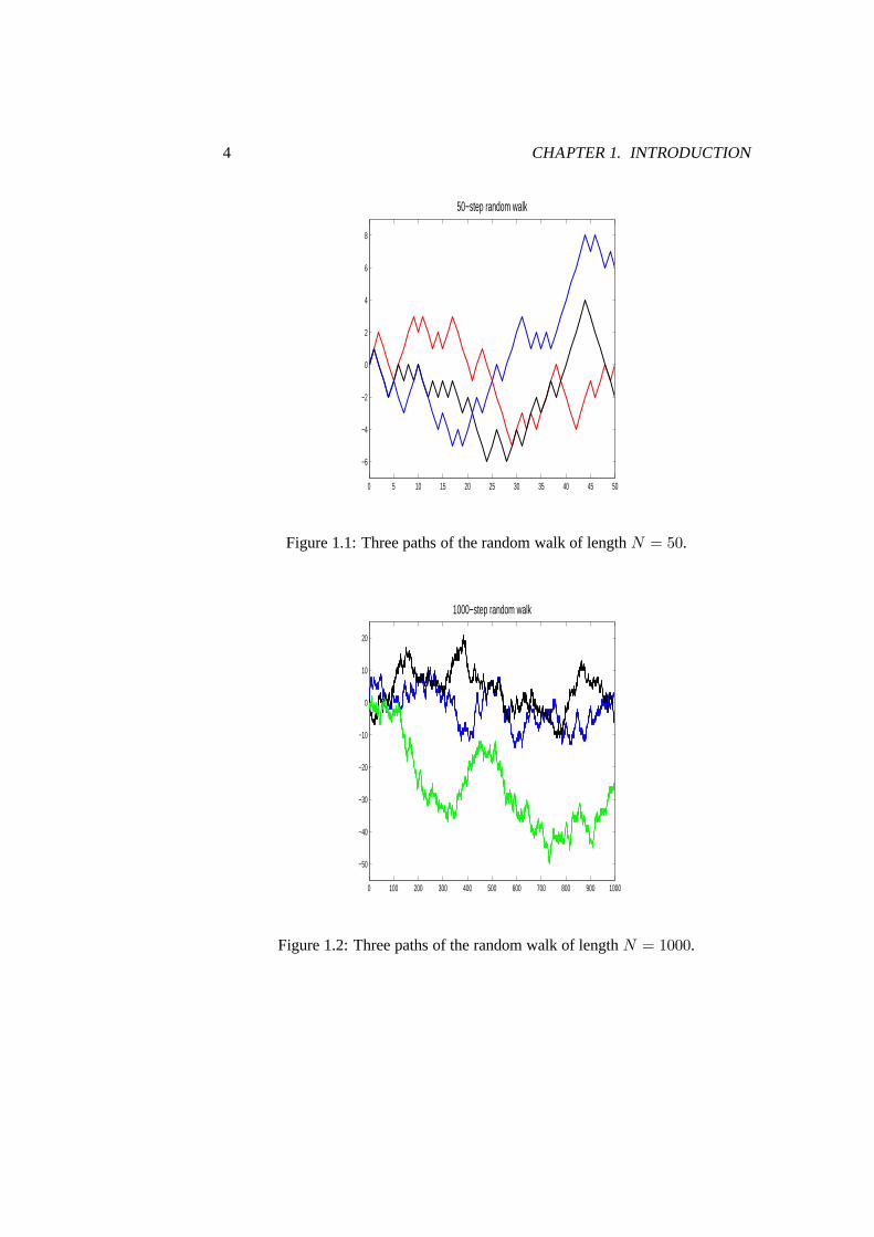
• The sequenceSnNn=1 indexed by the discrete timeT = 1, 2, . . . N is
the path of the random walk. We use a linear interpolation (i.e. connect thepointsn, Sn by straight lines) to generate a continuous path.
Every path of the random walk is different: it depends on the outcome of a se-quence of independent random experiments. We can compute statistics by gen-erating a large number of paths and computing averages. For example,E(Sn) =
0, E(S2n) = n. The paths of the random walk (without the linear interpolation) are
not continuous: the random walk has a jump of size1 at each time step. This is anexample of a discrete time, discrete space stochastic processes. The random walkis a time-homogeneous Markov process. If we take a large number of steps, therandom walk starts looking like a continuous time process with continuous paths.
4 CHAPTER 1. INTRODUCTION
0 5 10 15 20 25 30 35 40 45 50
−6
−4
−2
0
2
4
6
8
50−step random walk
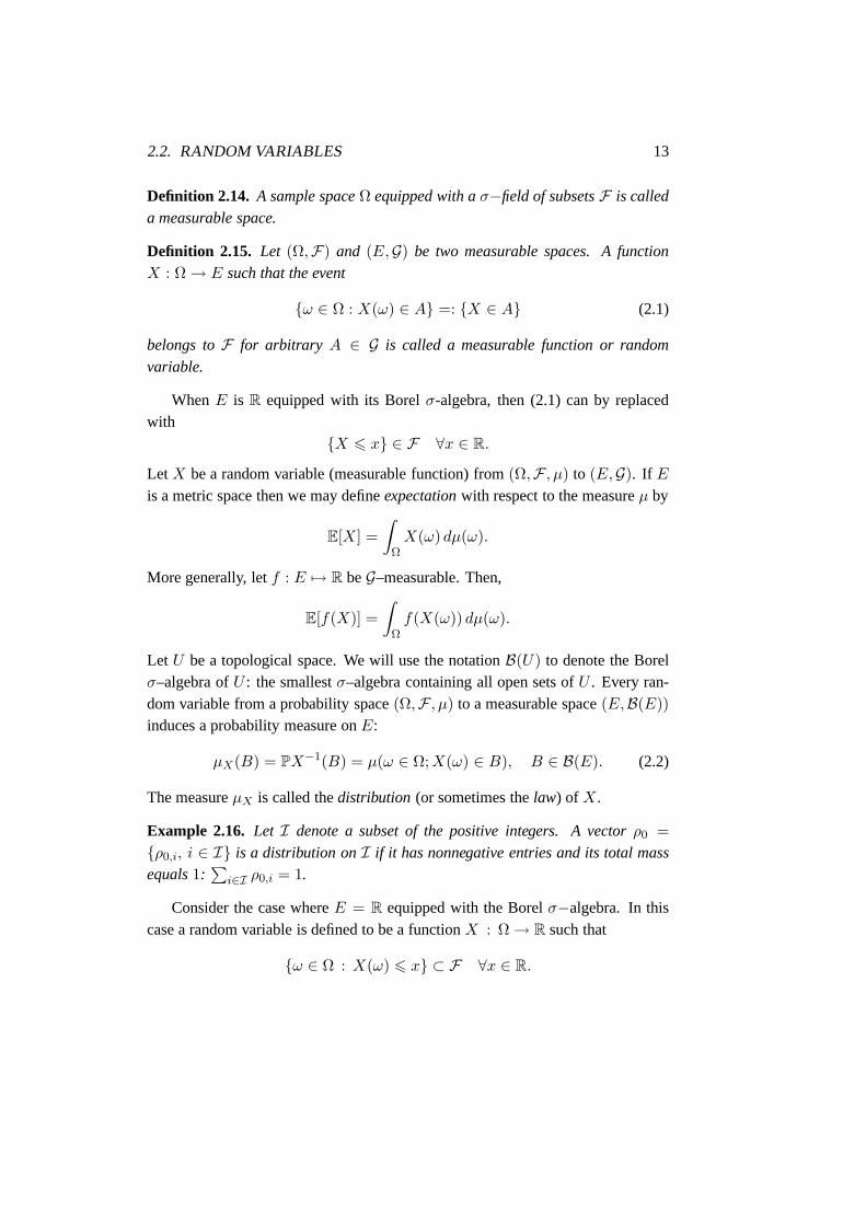
Figure 1.1: Three paths of the random walk of lengthN = 50.
0 100 200 300 400 500 600 700 800 900 1000
−50
−40
−30
−20
−10
0
10
20
1000−step random walk
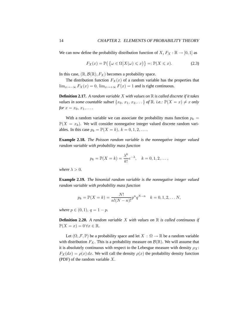
Figure 1.2: Three paths of the random walk of lengthN = 1000.
1.2. THE ONE-DIMENSIONAL RANDOM WALK 5
0 0.2 0.4 0.6 0.8 1−1.5
−1
−0.5
0
0.5
1
1.5
2
t
U(t)
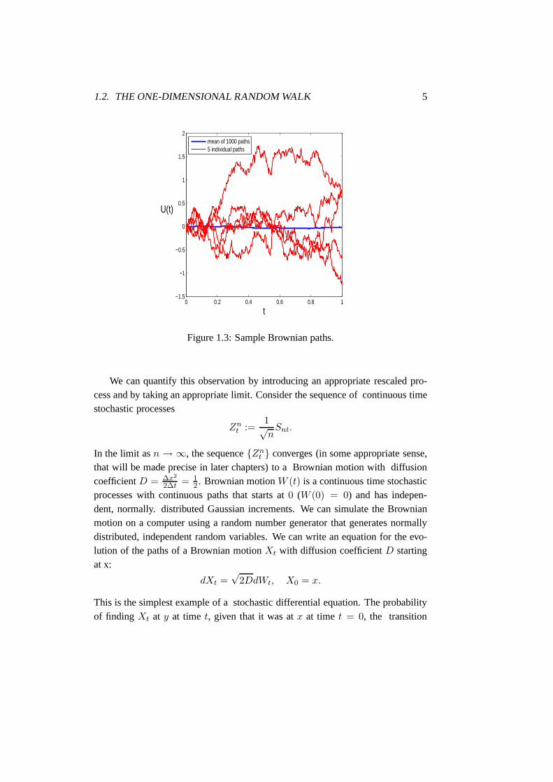
mean of 1000 paths5 individual paths
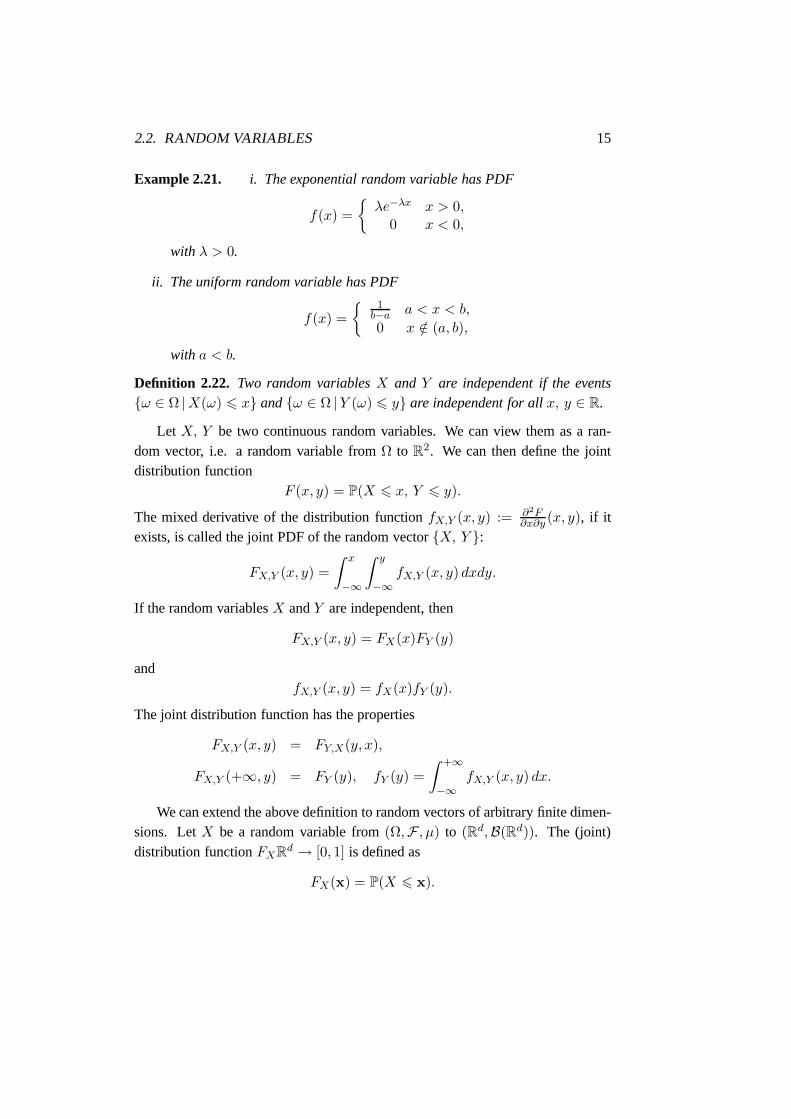
Figure 1.3: Sample Brownian paths.
We can quantify this observation by introducing an appropriate rescaled pro-cess and by taking an appropriate limit. Consider the sequence of continuous timestochastic processes
Znt :=
1√nSnt.
In the limit asn → ∞, the sequenceZnt converges (in some appropriate sense,
that will be made precise in later chapters) to a Brownian motion with diffusioncoefficientD = ∆x2
2∆t = 12 . Brownian motionW (t) is a continuous time stochastic
processes with continuous paths that starts at0 (W (0) = 0) and has indepen-dent, normally. distributed Gaussian increments. We can simulate the Brownianmotion on a computer using a random number generator that generates normallydistributed, independent random variables. We can write anequation for the evo-lution of the paths of a Brownian motionXt with diffusion coefficientD startingat x:
dXt =√
2DdWt, X0 = x.
This is the simplest example of a stochastic differential equation. The probabilityof finding Xt at y at time t, given that it was atx at time t = 0, the transition
6 CHAPTER 1. INTRODUCTION
probability densityρ(y, t) satisfies the PDE
∂ρ
∂t= D
∂2ρ
∂y2, ρ(y, 0) = δ(y − x).
This is the simplest example of the Fokker–Planck equation.The connection be-tween Brownian motion and the diffusion equation was made byEinstein in 1905.
1.3 Why Randomness
Why introduce randomness in the description of physical systems?
• To describe outcomes of a repeated set of experiments. Thinkof tossing acoin repeatedly or of throwing a dice.
• To describe a deterministic system for which we have incomplete informa-tion: we have imprecise knowledge of initial and boundary conditions or ofmodel parameters.
– ODEs with random initial conditions are equivalent to stochastic pro-cesses that can be described using stochastic differentialequations.
• To describe systems for which we are not confident about the validity of ourmathematical model.
• To describe a dynamical system exhibiting very complicatedbehavior (chaoticdynamical systems). Determinism versus predictability.
• To describe a high dimensional deterministic system using asimpler, lowdimensional stochastic system. Think of the physical modelfor Brownianmotion (a heavy particle colliding with many small particles).
• To describe a system that is inherently random. Think of quantum mechan-ics.
Stochastic modeling is currently used in many different areas ranging frombiology to climate modeling to economics.
1.4. DISCUSSION AND BIBLIOGRAPHY 7
1.4 Discussion and Bibliography
The fundamental papers of Einstein on the theory of Brownianmotion have beenreprinted by Dover [7]. The readers of this book are stronglyencouraged to studythese papers. Other fundamental papers from the early period of the developmentof the theory of stochastic processes include the papers by Langevin, Ornsteinand Uhlenbeck [25], Doob [5], Kramers [13] and Chandrashekhar’s famous re-view article [3]. Many of these early papers on the theory of stochastic processeshave been reprinted in [6]. Many of the early papers on the theory of Brown-ian motion are available fromhttp://www.physik.uni-augsburg.de/theo1/hanggi/History/BM-History.html. Very useful historical com-ments can be founds in the books by Nelson [19] and Mazo [18].
The figures in this chapter were generated using matlab programs fromhttp://www-math.bgsu.edu/z/sde/matlab/index.html.
1.5 Exercises
1. Read the papers by Einstein, Ornstein-Uhlenbeck, Doob etc.
2. Write a computer program for generating the random walk inone and two di-mensions. Study numerically the Brownian limit and computethe statistics ofthe random walk.

8 CHAPTER 1. INTRODUCTION

Chapter 2
Elements of Probability Theory
In this chapter we put together some basic definitions and results from probabilitytheory that will be used later on. In Section 2.1 we give some basic definitionsfrom the theory of probability. In Section 2.2 we present some properties of ran-dom variables. In Section 2.3 we introduce the concept of conditional expectationand in Section 2.4 we define the characteristic function, oneof the most usefultools in the study of (sums of) random variables. Some explicit calculations forthe multivariate Gaussian distribution are presented in Section 2.5. Different typesof convergence and the basic limit theorems of the theory of probability are dis-cussed in Section 2.6. Discussion and bibliographical comments are presented inSection 2.7. Exercises are included in Section 2.8.
2.1 Basic Definitions from Probability Theory
In Chapter 1 we defined a stochastic process as a dynamical system whose law ofevolution is probabilistic. In order to study stochastic processes we need to be ableto describe the outcome of a random experiment and to calculate functions of thisoutcome. First we need to describe the set of all possible experiments.
Definition 2.1. The set of all possible outcomes of an experiment is called thesample spaceand is denoted byΩ.
Example 2.2. • The possible outcomes of the experiment of tossing a coin areH andT . The sample space isΩ =
H, T
.
• The possible outcomes of the experiment of throwing a die are1, 2, 3, 4, 5
and6. The sample space isΩ =
1, 2, 3, 4, 5, 6
.
9
10 CHAPTER 2. ELEMENTS OF PROBABILITY THEORY
We defineeventsto be subsets of the sample space. Of course, we would likethe unions, intersections and complements of events to alsobe events. When thesample spaceΩ is uncountable, then technical difficulties arise. In particular, notall subsets of the sample space need to be events. A definitionof the collection ofsubsets of events which is appropriate for finite additive probability is the follow-ing.
Definition 2.3. A collectionF of Ω is called a field onΩ if
i. ∅ ∈ F ;
ii. if A ∈ F thenAc ∈ F ;
iii. If A, B ∈ F thenA ∪B ∈ F .
From the definition of a field we immediately deduce thatF is closed underfinite unions and finite intersections:
A1, . . . An ∈ F ⇒ ∪ni=1Ai ∈ F , ∩n
i=1Ai ∈ F .
When Ω is infinite dimensional then the above definition is not appropriatesince we need to consider countable unions of events.
Definition 2.4 (σ−algebra). A collectionF of Ω is called aσ-field or σ-algebraonΩ if
i. ∅ ∈ F ;
ii. if A ∈ F thenAc ∈ F ;
iii. If A1, A2, · · · ∈ F then∪∞i=1Ai ∈ F .
A σ-algebra is closed under the operation of taking countable intersections.
Example 2.5. • F =
∅, Ω
.
• F =
∅, A, Ac, Ω
whereA is a subset ofΩ.
• The power set ofΩ, denoted by0, 1Ω which contains all subsets ofΩ.
Let F be a collection of subsets ofΩ. It can be extended to aσ−algebra (takefor example the power set ofΩ). Consider all theσ−algebras that containF andtake their intersection, denoted byσ(F), i.e. A ⊂ Ω if and only if it is in everyσ−algebra containingF . σ(F) is aσ−algebra (see Exercise 1 ). It is the smallestalgebra containingF and it is called theσ−algebra generated byF .
2.1. BASIC DEFINITIONS FROM PROBABILITY THEORY 11
Example 2.6. Let Ω = Rn. Theσ-algebra generated by the open subsets ofR
n
(or, equivalently, by the open balls ofRn) is called the Borelσ-algebra ofRn and
is denoted byB(Rn).
LetX be a closed subset ofRn. Similarly, we can define the Borelσ-algebra
of X, denoted byB(X).A sub-σ–algebra is a collection of subsets of aσ–algebra which satisfies the
axioms of aσ–algebra.Theσ−field F of a sample spaceΩ contains all possible outcomes of the ex-
periment that we want to study. Intuitively, theσ−field contains all the informationabout the random experiment that is available to us.
Now we want to assign probabilities to the possible outcomesof an experiment.
Definition 2.7 (Probability measure). A probability measureP on the measurablespace(Ω, F) is a functionP : F 7→ [0, 1] satisfying
i. P(∅) = 0, P(Ω) = 1;
ii. For A1, A2, . . . withAi ∩Aj = ∅, i 6= j then
P(∪∞i=1Ai) =
∞∑
i=1
P(Ai).
Definition 2.8. The triple(
Ω, F , P)
comprising a setΩ, aσ-algebraF of subsetsof Ω and a probability measureP on (Ω, F) is a called a probability space.
Example 2.9. A biased coin is tossed once:Ω = H, T, F = ∅, H, T, Ω =
0, 1, P : F 7→ [0, 1] such thatP(∅) = 0, P(H) = p ∈ [0, 1], P(T ) =
1 − p, P(Ω) = 1.
Example 2.10. TakeΩ = [0, 1], F = B([0, 1]), P = Leb([0, 1]). Then(Ω,F ,P)
is a probability space.
2.1.1 Conditional Probability
One of the most important concepts in probability is that of the dependence be-tween events.
Definition 2.11. A familyAi : i ∈ I of events is called independent if
P(
∩j∈J Aj
)
= Πj∈JP(Aj)
for all finite subsetsJ of I.
12 CHAPTER 2. ELEMENTS OF PROBABILITY THEORY
When two eventsA, B are dependent it is important to know the probabilitythat the eventA will occur, given thatB has already happened. We define this tobeconditional probability, denoted byP(A|B). We know from elementary proba-bility that
P (A|B) =P (A ∩B)
P(B).
A very useful result is that of thelaw of total probability.
Definition 2.12. A family of eventsBi : i ∈ I is called a partition ofΩ if
Bi ∩Bj = ∅, i 6= j and ∪i∈I Bi = Ω.
Proposition 2.13. Law of total probability. For any eventA and any partitionBi : i ∈ I we have
P(A) =∑
i∈I
P(A|Bi)P(Bi).
The proof of this result is left as an exercise. In many cases the calculation ofthe probability of an event is simplified by choosing an appropriate partition ofΩand using the law of total probability.
Let (Ω,F ,P) be a probability space and fixB ∈ F . ThenP(·|B) defines aprobability measure onF . Indeed, we have that
P(∅|B) = 0, P(Ω|B) = 1
and (sinceAi ∩Aj = ∅ implies that(Ai ∩B) ∩ (Aj ∩B) = ∅)
P (∪∞j=1Ai|B) =
∞∑
j=1
P(Ai|B),
for a countable family of pairwise disjoint setsAj+∞j=1. Consequently,(Ω,F ,P(·|B))
is a probability space for everyB ∈ cF .
2.2 Random Variables
We are usually interested in the consequences of the outcomeof an experiment,rather than the experiment itself. The function of the outcome of an experiment isa random variable, that is, a map fromΩ to R.
2.2. RANDOM VARIABLES 13
Definition 2.14. A sample spaceΩ equipped with aσ−field of subsetsF is calleda measurable space.
Definition 2.15. Let (Ω,F) and (E,G) be two measurable spaces. A functionX : Ω → E such that the event
ω ∈ Ω : X(ω) ∈ A =: X ∈ A (2.1)
belongs toF for arbitrary A ∈ G is called a measurable function or randomvariable.
WhenE is R equipped with its Borelσ-algebra, then (2.1) can by replacedwith
X 6 x ∈ F ∀x ∈ R.
LetX be a random variable (measurable function) from(Ω,F , µ) to (E,G). If Eis a metric space then we may defineexpectationwith respect to the measureµ by
E[X] =
∫
ΩX(ω) dµ(ω).
More generally, letf : E 7→ R beG–measurable. Then,
E[f(X)] =
∫
Ωf(X(ω)) dµ(ω).
Let U be a topological space. We will use the notationB(U) to denote the Borelσ–algebra ofU : the smallestσ–algebra containing all open sets ofU . Every ran-dom variable from a probability space(Ω,F , µ) to a measurable space(E,B(E))
induces a probability measure onE:
µX(B) = PX−1(B) = µ(ω ∈ Ω;X(ω) ∈ B), B ∈ B(E). (2.2)
The measureµX is called thedistribution (or sometimes thelaw) of X.
Example 2.16. Let I denote a subset of the positive integers. A vectorρ0 =
ρ0,i, i ∈ I is a distribution onI if it has nonnegative entries and its total massequals1:
∑
i∈I ρ0,i = 1.
Consider the case whereE = R equipped with the Borelσ−algebra. In thiscase a random variable is defined to be a functionX : Ω → R such that
ω ∈ Ω : X(ω) 6 x ⊂ F ∀x ∈ R.
14 CHAPTER 2. ELEMENTS OF PROBABILITY THEORY
We can now define the probability distribution function ofX, FX : R → [0, 1] as
FX(x) = P(
ω ∈ Ω∣
∣X(ω) 6 x)
=: P(X 6 x). (2.3)
In this case,(R,B(R), FX) becomes a probability space.
The distribution functionFX(x) of a random variable has the properties thatlimx→−∞ FX(x) = 0, limx→+∞ F (x) = 1 and is right continuous.
Definition 2.17. A random variableX with values onR is called discrete if it takesvalues in some countable subsetx0, x1, x2, . . . of R. i.e.: P(X = x) 6= x onlyfor x = x0, x1, . . . .
With a random variable we can associate the probability massfunction pk =
P(X = xk). We will consider nonnegative integer valued discrete random vari-ables. In this casepk = P(X = k), k = 0, 1, 2, . . . .
Example 2.18. The Poisson random variable is the nonnegative integer valuedrandom variable with probability mass function
pk = P(X = k) =λk
k!e−λ, k = 0, 1, 2, . . . ,
whereλ > 0.
Example 2.19. The binomial random variable is the nonnegative integer valuedrandom variable with probability mass function
pk = P(X = k) =N !
n!(N − n)!pnqN−n k = 0, 1, 2, . . . N,
wherep ∈ (0, 1), q = 1 − p.
Definition 2.20. A random variableX with values onR is called continuous ifP(X = x) = 0∀x ∈ R.
Let (Ω,F ,P) be a probability space and letX : Ω → R be a random variablewith distributionFX . This is a probability measure onB(R). We will assume thatit is absolutely continuous with respect to the Lebesgue measure with densityρX :FX(dx) = ρ(x) dx. We will call the densityρ(x) the probability density function(PDF) of the random variableX.
2.2. RANDOM VARIABLES 15
Example 2.21. i. The exponential random variable has PDF
f(x) =
λe−λx x > 0,0 x < 0,
with λ > 0.
ii. The uniform random variable has PDF
f(x) =
1b−a a < x < b,
0 x /∈ (a, b),
with a < b.
Definition 2.22. Two random variablesX and Y are independent if the eventsω ∈ Ω |X(ω) 6 x andω ∈ Ω |Y (ω) 6 y are independent for allx, y ∈ R.
Let X, Y be two continuous random variables. We can view them as a ran-dom vector, i.e. a random variable fromΩ to R
2. We can then define the jointdistribution function
F (x, y) = P(X 6 x, Y 6 y).
The mixed derivative of the distribution functionfX,Y (x, y) := ∂2F∂x∂y (x, y), if it
exists, is called the joint PDF of the random vectorX, Y :
FX,Y (x, y) =
∫ x
−∞
∫ y
−∞fX,Y (x, y) dxdy.
If the random variablesX andY are independent, then
FX,Y (x, y) = FX(x)FY (y)
andfX,Y (x, y) = fX(x)fY (y).
The joint distribution function has the properties
FX,Y (x, y) = FY,X(y, x),
FX,Y (+∞, y) = FY (y), fY (y) =
∫ +∞
−∞fX,Y (x, y) dx.
We can extend the above definition to random vectors of arbitrary finite dimen-sions. LetX be a random variable from(Ω,F , µ) to (Rd,B(Rd)). The (joint)distribution functionFXR
d → [0, 1] is defined as
FX(x) = P(X 6 x).
16 CHAPTER 2. ELEMENTS OF PROBABILITY THEORY
Let X be a random variable inRd with distribution functionf(xN ) wherexN =
x1, . . . xN. We define the marginal or reduced distribution functionfN−1(xN−1)
by
fN−1(xN−1) =
∫
R
fN(xN ) dxN .
We can define other reduced distribution functions:
fN−2(xN−2) =
∫
R
fN−1(xN−1) dxN−1 =
∫
R
∫
R
f(xN ) dxN−1dxN .
2.2.1 Expectation of Random Variables
We can use the distribution of a random variable to compute expectations and prob-abilities:
E[f(X)] =
∫
R
f(x) dFX (x) (2.4)
and
P[X ∈ G] =
∫
GdFX(x), G ∈ B(E). (2.5)
The above formulas apply to both discrete and continuous random variables, pro-vided that we define the integrals in (2.4) and (2.5) appropriately.
WhenE = Rd and a PDF exists,dFX(x) = fX(x) dx, we have
FX(x) := P(X 6 x) =
∫ x1
−∞. . .
∫ xd
−∞fX(x) dx..
WhenE = Rd then byLp(Ω; Rd), or sometimesLp(Ω;µ) or even simplyLp(µ),
we mean the Banach space of measurable functions onΩ with norm
‖X‖Lp =(
E|X|p)1/p
.
LetX be a nonnegative integer valued random variable with probability massfunction pk. We can compute the expectation of an arbitrary function ofX usingthe formula
E(f(X)) =
∞∑
k=0
f(k)pk.
Let X, Y be random variables we want to know whether they are correlatedand, if they are, to calculate how correlated they are. We define the covariance ofthe two random variables as
cov(X,Y ) = E[
(X − EX)(Y − EY )]
= E(XY ) − EXEY.

2.2. RANDOM VARIABLES 17
The correlation coefficient is
ρ(X,Y ) =cov(X,Y )
√
var(X)√
var(X)(2.6)
The Cauchy-Schwarz inequality yields thatρ(X,Y ) ∈ [−1, 1]. We will saythat two random variablesX andY are uncorrelated provided thatρ(X,Y ) = 0. Itis not true in general that two uncorrelated random variables are independent. Thisis true, however, for Gaussian random variables (see Exercise 5).
Example 2.23. • Consider the random variableX : Ω 7→ R with pdf
γσ,b(x) := (2πσ)−1
2 exp
(
−(x− b)2
2σ
)
.
Such anX is termed a Gaussian or normal random variable. The mean is
EX =
∫
R
xγσ,b(x) dx = b
and the variance is
E(X − b)2 =
∫
R
(x− b)2γσ,b(x) dx = σ.
• Let b ∈ Rd andΣ ∈ R
d×d be symmetric and positive definite. The randomvariableX : Ω 7→ R
d with pdf
γΣ,b(x) :=(
(2π)ddetΣ)− 1
2
exp
(
−1
2〈Σ−1(x− b), (x − b)〉
)
is termed a multivariate Gaussian or normal random variable. The mean is
E(X) = b (2.7)
and the covariance matrix is
E
(
(X − b) ⊗ (X − b))
= Σ. (2.8)
Since the mean and variance specify completely a Gaussian random variable onR, the Gaussian is commonly denoted byN (m,σ). The standard normal randomvariable isN (0, 1). Similarly, since the mean and covariance matrix completelyspecify a Gaussian random variable onR
d, the Gaussian is commonly denoted byN (m,Σ).
Some analytical calculations for Gaussian random variables will be presentedin Section 2.5.
18 CHAPTER 2. ELEMENTS OF PROBABILITY THEORY
2.3 Conditional Expecation
Assume thatX ∈ L1(Ω,F , µ) and letG be a sub–σ–algebra ofF . The conditionalexpectation ofX with respect toG is defined to be the function (random variable)E[X|G] : Ω 7→ E which isG–measurable and satisfies
∫
GE[X|G] dµ =
∫
GX dµ ∀G ∈ G.
We can defineE[f(X)|G] and the conditional probabilityP[X ∈ F |G] = E[IF (X)|G],whereIF is the indicator function ofF , in a similar manner.
We list some of the most important properties of conditionalexpectation.
Theorem 2.24. [Properties of Conditional Expectation]. Let(Ω,F , µ) be a prob-ability space and letG be a sub–σ–algebra ofF .
(a) If X is G−measurable and integrable thenE(X|G) = X.
(b) (Linearity) IfX1, X2 are integrable andc1, c2 constants, then
E(c1X1 + c2X2|G) = c1E(X1|G) + c2E(X2|G).
(c) (Order) IfX1, X2 are integrable andX1 6 X2 a.s., thenE(X1|G) 6 E(X2|G)
a.s.
(d) If Y andXY are integrable, andX is G−measurable thenE(XY |G) =
XE(Y |G).
(e) (Successive smoothing) IfD is a sub–σ–algebra ofF , D ⊂ G andX is inte-grable, thenE(X|D) = E[E(X|G)|D] = E[E(X|D)|G].
(f) (Convergence) LetXn∞n=1 be a sequence of random variables such that, forall n, |Xn| 6 Z whereZ is integrable. IfXn → X a.s., thenE(Xn|G) →E(X|G) a.s. and inL1.
Proof. See Exercise 10.
2.4 The Characteristic Function
Many of the properties of (sums of) random variables can be studied using theFourier transform of the distribution function. LetF (λ) be the distribution function

2.5. GAUSSIAN RANDOM VARIABLES 19
of a (discrete or continuous) random variableX. The characteristic function ofXis defined to be the Fourier transform of the distribution function
φ(t) =
∫
R
eitλ dF (λ) = E(eitX ). (2.9)
For a continuous random variable for which the distributionfunctionF has a den-sity, dF (λ) = p(λ)dλ, (2.9) gives
φ(t) =
∫
R
eitλp(λ) dλ.
For a discrete random variable for whichP(X = λk) = αk, (2.9) gives
φ(t) =∞∑
k=0
eitλkak.
From the properties of the Fourier transform we conclude that the characteristicfunction determines uniquely the distribution function ofthe random variable, inthe sense that there is a one-to-one correspondance betweenF (λ) andφ(t). Fur-thermore, in the exercises at the end of the chapter the reader is asked to prove thefollowing two results.
Lemma 2.25. Let X1,X2, . . . Xn be independent random variables with char-acteristic functionsφj(t), j = 1, . . . n and letY =
∑nj=1Xj with characteristic
functionφY (t). Then
φY (t) = Πnj=1φj(t).
Lemma 2.26. LetX be a random variable with characteristic functionφ(t) andassume that it has finite moments. Then
E(Xk) =1
ikφ(k)(0).
2.5 Gaussian Random Variables
In this section we present some useful calculations for Gaussian random variables.In particular, we calculate the normalization constant, the mean and variance andthe characteristic function of multidimensional Gaussianrandom variables.

20 CHAPTER 2. ELEMENTS OF PROBABILITY THEORY
Theorem 2.27.Letb ∈ Rd andΣ ∈ R
d×d a symmetric and positive definite ma-trix. Let X be the multivariate Gaussian random variable with probability densityfunction
γΣ,b(x) =1
Zexp
(
−1
2〈Σ−1(x − b),x − b〉
)
.
Then
i. The normalization constant is
Z = (2π)d/2√
det(Σ).
ii. The mean vector and covariance matrix ofX are given by
EX = b
and
E((X − EX) ⊗ (X − EX)) = Σ.
iii. The characteristic function ofX is
φ(t) = ei〈b,t〉− 1
2〈t,Σt〉.
Proof. i. From the spectral theorem for symmetric positive definitematriceswe have that there exists a diagonal matrixΛ with positive entries and anorthogonal matrixB such that
Σ−1 = BT Λ−1B.
Let z = x− b andy = Bz. We have
〈Σ−1z, z〉 = 〈BT Λ−1Bz, z〉= 〈Λ−1Bz, Bz〉 = 〈Λ−1y,y〉
=
d∑
i=1
λ−1i y2
i .
Furthermore, we have that det(Σ−1) = Πdi=1λ
−1i , that det(Σ) = Πd
i=1λi
and that the Jacobian of an orthogonal transformation isJ = det(B) = 1.
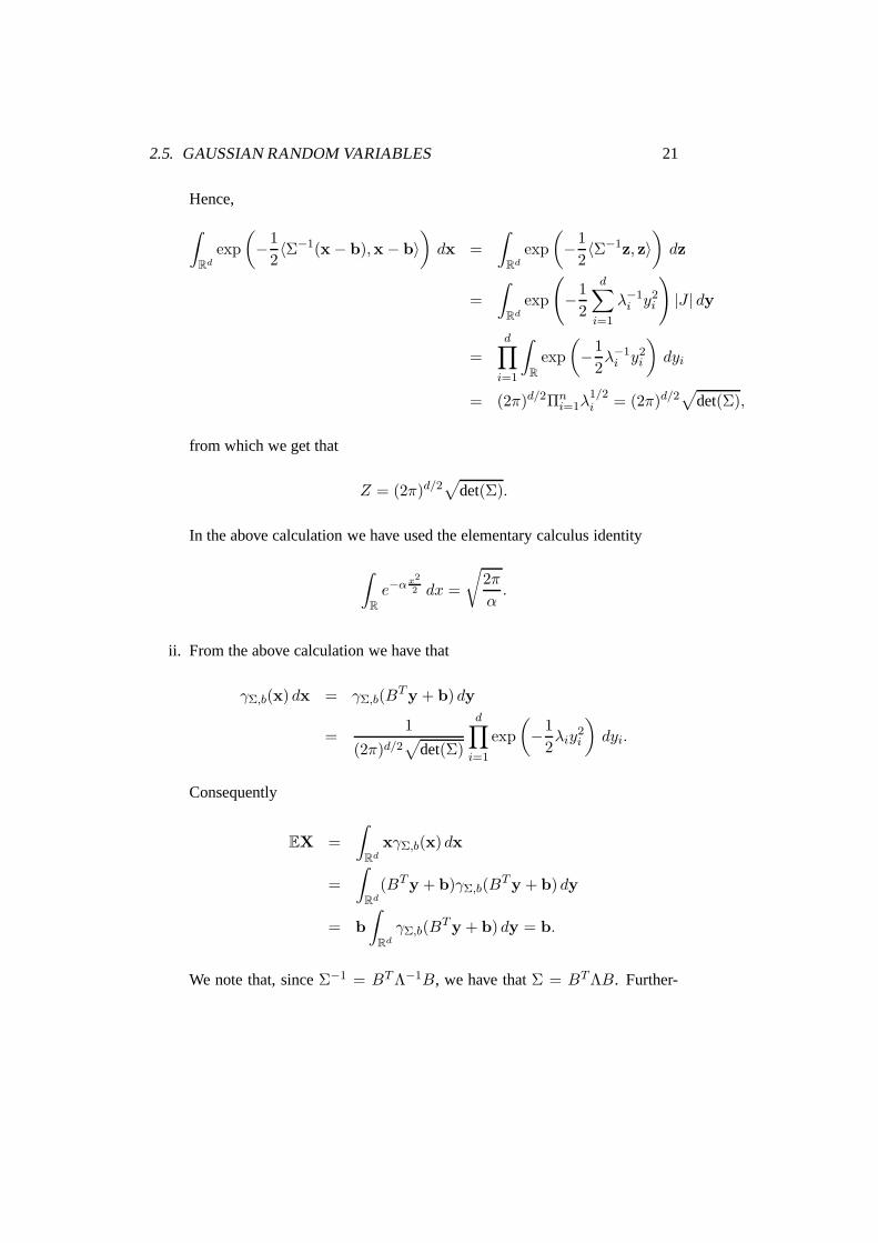
2.5. GAUSSIAN RANDOM VARIABLES 21
Hence,
∫
Rd
exp
(
−1
2〈Σ−1(x − b),x − b〉
)
dx =
∫
Rd
exp
(
−1
2〈Σ−1z, z〉
)
dz
=
∫
Rd
exp
(
−1
2
d∑
i=1
λ−1i y2
i
)
|J | dy
=d∏
i=1
∫
R
exp
(
−1
2λ−1
i y2i
)
dyi
= (2π)d/2Πni=1λ
1/2i = (2π)d/2
√
det(Σ),
from which we get that
Z = (2π)d/2√
det(Σ).
In the above calculation we have used the elementary calculus identity
∫
R
e−α x2
2 dx =
√
2π
α.
ii. From the above calculation we have that
γΣ,b(x) dx = γΣ,b(BTy + b) dy
=1
(2π)d/2√
det(Σ)
d∏
i=1
exp
(
−1
2λiy
2i
)
dyi.
Consequently
EX =
∫
Rd
xγΣ,b(x) dx
=
∫
Rd
(BTy + b)γΣ,b(BTy + b) dy
= b
∫
Rd
γΣ,b(BTy + b) dy = b.
We note that, sinceΣ−1 = BT Λ−1B, we have thatΣ = BTΛB. Further-
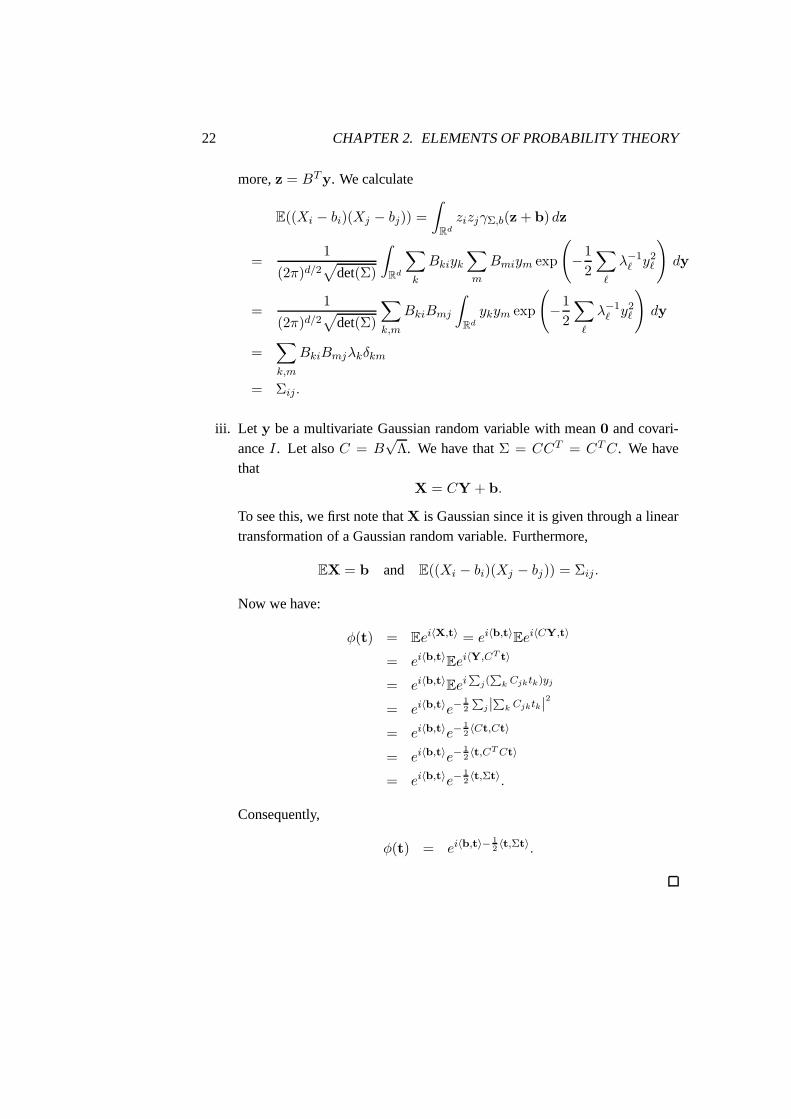
22 CHAPTER 2. ELEMENTS OF PROBABILITY THEORY
more,z = BTy. We calculate
E((Xi − bi)(Xj − bj)) =
∫
Rd
zizjγΣ,b(z + b) dz
=1
(2π)d/2√
det(Σ)
∫
Rd
∑
k
Bkiyk
∑
m
Bmiym exp
(
−1
2
∑
ℓ
λ−1ℓ y2
ℓ
)
dy
=1
(2π)d/2√
det(Σ)
∑
k,m
BkiBmj
∫
Rd
ykym exp
(
−1
2
∑
ℓ
λ−1ℓ y2
ℓ
)
dy
=∑
k,m
BkiBmjλkδkm
= Σij.
iii. Let y be a multivariate Gaussian random variable with mean0 and covari-anceI. Let alsoC = B
√Λ. We have thatΣ = CCT = CTC. We have
thatX = CY + b.
To see this, we first note thatX is Gaussian since it is given through a lineartransformation of a Gaussian random variable. Furthermore,
EX = b and E((Xi − bi)(Xj − bj)) = Σij.
Now we have:
φ(t) = Eei〈X,t〉 = ei〈b,t〉Eei〈CY,t〉
= ei〈b,t〉Eei〈Y,CT t〉
= ei〈b,t〉Eei
P
j(P
k Cjktk)yj
= ei〈b,t〉e−1
2
P
j|Pk Cjktk|2
= ei〈b,t〉e−1
2〈Ct,Ct〉
= ei〈b,t〉e−1
2〈t,CT Ct〉
= ei〈b,t〉e−1
2〈t,Σt〉.
Consequently,
φ(t) = ei〈b,t〉− 1
2〈t,Σt〉.
2.6. TYPES OF CONVERGENCE AND LIMIT THEOREMS 23
2.6 Types of Convergence and Limit Theorems
One of the most important aspects of the theory of random variables is the study oflimit theorems for sums of random variables. The most well known limit theoremsin probability theory are the law of large numbers and the central limit theorem.There are various different types of convergence for sequences or random variables.We list the most important types of convergence below.
Definition 2.28. LetZn∞n=1 be a sequence of random variables. We will say that
(a) Zn converges toZ with probability one if
P(
limn→+∞
Zn = Z)
= 1.
(b) Zn converges toZ in probability if for everyε > 0
limn→+∞
P(
|Zn − Z| > ε)
= 0.
(c) Zn converges toZ in Lp if
limn→+∞
E[∣
∣Zn − Z∣
∣
p]= 0.
(d) Let Fn(λ), n = 1, · · · + ∞, F (λ) be the distribution functions ofZn n =
1, · · · + ∞ andZ, respectively. ThenZn converges toZ in distribution if
limn→+∞
Fn(λ) = F (λ)
for all λ ∈ R at whichF is continuous.
Recall that the distribution functionFX of a random variable from a probabilityspace(Ω,F ,P) to R induces a probability measure onR and that(R,B(R), FX ) isa probability space. We can show that the convergence in distribution is equivalentto the weak convergence of the probability measures inducedby the distributionfunctions.
Definition 2.29. Let (E, d) be a metric space,B(E) theσ−algebra of its Borelsets,Pn a sequence of probability measures on(E,B(E)) and letCb(E) denotethe space of bounded continuous functions onE. We will say that the sequence ofPn converges weakly to the probability measureP if, for eachf ∈ Cb(E),
limn→+∞
∫
Ef(x) dPn(x) =
∫
Ef(x) dP (x).

24 CHAPTER 2. ELEMENTS OF PROBABILITY THEORY
Theorem 2.30.LetFn(λ), n = 1, · · · + ∞, F (λ) be the distribution functions ofZn n = 1, · · · + ∞ andZ, respectively. ThenZn converges toZ in distribution ifand only if, for allg ∈ Cb(R)
limn→+∞
∫
Xg(x) dFn(x) =
∫
Xg(x) dF (x). (2.10)
Notice that (2.10) is equivalent to
limn→+∞
Eng(Xn) = Eg(X),
whereEn andE denote the expectations with respect toFn andF , respectively.
When the sequence of random variables whose convergence we are interestedin takes values inRd or, more generally, a metric space space(E, d) then we canuse weak convergence of the sequence of probability measures induced by thesequence of random variables to define convergence in distribution.
Definition 2.31. A sequence of real valued random variablesXn defined on aprobability spaces(Ωn,Fn, Pn) and taking values on a metric space(E, d) is saidto converge in distribution if the indued measuresFn(B) = Pn(Xn ∈ B) forB ∈ B(E) converge weakly to a probability measureP .
Let Xn∞n=1 be iid random variables withEXn = V . Then, thestrong lawof large numbersstates that average of the sum of the iid converges toV withprobability one:
P
(
limN→+∞
1
N
N∑
n=1
Xn = V)
= 1.
The strong law of large numbers provides us with informationabout the behav-ior of a sum of random variables (or, a large number or repetitions of the sameexperiment) on average. We can also study fluctuations around the average be-havior. Indeed, letE(Xn − V )2 = σ2. Define the centered iid random variablesYn = Xn − V . Then, the sequence of random variables1
σ√
N
∑Nn=1 Yn converges
in distribution to aN (0, 1) random variable:
limn→+∞
P
(
1
σ√N
N∑
n=1
Yn 6 a
)
=
∫ a
−∞
1√2πe−
1
2x2
dx.
This is thecentral limit theorem.
2.7. DISCUSSION AND BIBLIOGRAPHY 25
2.7 Discussion and Bibliography
The material of this chapter is very standard and can be foundin many books onprobability theory. Well known textbooks on probability theory are [2, 8, 9, 16, 17,12, 23].
The connection between conditional expectation and orthogonal projections isdiscussed in [4].
The reduced distribution functions defined in Section 2.2 are used extensivelyin statistical mechanics. A different normalization is usually used in physics text-books. See for instance [1, Sec. 4.2].
The calculations presented in Section 2.5 are essentially an exercise in linearalgebra. See [15, Sec. 10.2].
Random variables and probability measures can also be defined in infinite di-mensions. More information can be found in [20, Ch. 2].
The study of limit theorems is one of the cornerstones of probability theory andof the theory of stochastic processes. A comprehensive study of limit theorems canbe found in [10].
2.8 Exercises
1. Show that the intersection of a family ofσ-algebras is aσ-algebra.
2. Prove the law of total probability, Proposition 2.13.
3. Calculate the mean, variance and characteristic function of the following prob-ability density functions.
(a) The exponential distribution with density
f(x) =
λe−λx x > 0,0 x < 0,
with λ > 0.
(b) The uniform distribution with density
f(x) =
1b−a a < x < b,
0 x /∈ (a, b),
with a < b.
26 CHAPTER 2. ELEMENTS OF PROBABILITY THEORY
(c) The Gamma distribution with density
f(x) =
λΓ(α)(λx)
α−1e−λx x > 0,
0 x < 0,
with λ > 0, α > 0 andΓ(α) is the Gamma function
Γ(α) =
∫ ∞
0ξα−1e−ξ dξ, α > 0.
4. LeX andY be independent random variables with distribution functionsFX
andFY . Show that the distribution function of the sumZ = X + Y is theconvolution ofFX andFY :
FZ(x) =
∫
FX(x− y) dFY (y).
5. LetX andY be Gaussian random variables. Show that they are uncorrelated ifand only if they are independent.
6. (a) LetX be a continuous random variable with characteristic function φ(t).Show that
EXk =1
ikφ(k)(0),
whereφ(k)(t) denotes thek-th derivative ofφ evaluated att.
(b) LetX be a nonnegative random variable with distribution function F (x).Show that
E(X) =
∫ +∞
0(1 − F (x)) dx.
(c) LetX be a continuous random variable with probability density functionf(x) and characteristic functionφ(t). Find the probability density andcharacteristic function of the random variableY = aX+ b with a, b ∈ R.
(d) LetX be a random variable with uniform distribution on[0, 2π]. Find theprobability density of the random variableY = sin(X).
7. LetX be a discrete random variable taking vales on the set of nonnegative inte-gers with probability mass functionpk = P(X = k) with pk > 0,
∑+∞k=0 pk =
1. Thegenerating functionis defined as
g(s) = E(sX) =+∞∑
k=0
pksk.
2.8. EXERCISES 27
(a) Show that
EX = g′(1) and EX2 = g′′(1) + g′(1),
where the prime denotes differentiation.
(b) Calculate the generating function of the Poisson randomvariable with
pk = P(X = k) =e−λλk
k!, k = 0, 1, 2, . . . and λ > 0.
(c) Prove that the generating function of a sum of independent nonnegativeinteger valued random variables is the product of their generating func-tions.
8. Write a computer program for studying the law of large numbers and the centrallimit theorem. Investigate numerically the rate of convergence of these twotheorems.
9. Study the properties of Gaussian measures on separable Hilbert spaces from [20,Ch. 2].
10. Prove Theorem 2.24.

28 CHAPTER 2. ELEMENTS OF PROBABILITY THEORY
Chapter 3
Basics of the Theory of StochasticProcesses
In this chapter we present some basic results form the theoryof stochastic pro-cesses and we investigate the properties of some of the standard stochastic pro-cesses in continuous time. In Section 3.1 we give the definition of a stochastic pro-cess. In Section 3.2 we present some properties of stationary stochastic processes.In Section 3.3 we introduce Brownian motion and study some ofits properties.Various examples of stochastic processes in continuous time are presented in Sec-tion 3.4. The Karhunen-Loeve expansion, one of the most useful tools for repre-senting stochastic processes and random fields, is presented in Section 3.5. Furtherdiscussion and bibliographical comments are presented in Section 3.6. Section 3.7contains exercises.
3.1 Definition of a Stochastic Process
Stochastic processes describe dynamical systems whose evolution law is of proba-bilistic nature. The precise definition is given below.
Definition 3.1 (stochastic process). LetT be an ordered set,(Ω,F ,P) a probabil-ity space and(E,G) a measurable space. A stochastic process is a collection ofrandom variablesX = Xt; t ∈ T where, for each fixedt ∈ T , Xt is a randomvariable from(Ω,F ,P) to (E,G). Ω is called the sample space. andE is the statespace of the stochastic processXt.
The setT can be either discrete, for example the set of positive integersZ+, or
29

30 CHAPTER 3. BASICS OF THE THEORY OF STOCHASTIC PROCESSES
continuous,T = [0,+∞). The state spaceE will usually beRd equipped with the
σ–algebra of Borel sets.A stochastic processX may be viewed as a function of botht ∈ T andω ∈ Ω.
We will sometimes writeX(t),X(t, ω) orXt(ω) instead ofXt. For a fixed samplepoint ω ∈ Ω, the functionXt(ω) : T 7→ E is called a (realization, trajectory) ofthe processX.
Definition 3.2 (finite dimensional distributions). The finite dimensional distribu-tions (fdd) of a stochastic process are the distributions oftheEk–valued randomvariables(X(t1),X(t2), . . . ,X(tk)) for arbitrary positive integerk and arbitrarytimesti ∈ T, i ∈ 1, . . . , k:
F (x) = P(X(ti) 6 xi, i = 1, . . . , k)
with x = (x1, . . . , xk).
From experiments or numerical simulations we can only obtain informationabout the finite dimensional distributions of a process. A natural question arises:are the finite dimensional distributions of a stochastic process sufficient to deter-mine a stochastic process uniquely? This is true for processes with continuouspaths1. This is the class of stochastic processes that we will studyin these notes.
Definition 3.3. We will say that two processesXt and Yt are equivalent if theyhave same finite dimensional distributions.
Definition 3.4. A one dimensional continuous time Gaussian process is a stochas-tic process for whichE = R and all the finite dimensional distributions are Gaus-sian, i.e. every finite dimensional vector(Xt1 ,Xt2 , . . . ,Xtk ) is aN (µk,Kk) ran-
dom variable for some vectorµk and a symmetric nonnegative definite matrixKk
for all k = 1, 2, . . . and for all t1, t2, . . . , tk.
From the above definition we conclude that the finite dimensional distributionsof a Gaussian continuous time stochastic process are Gaussian with probabilitydistribution function
γµk ,Kk(x) = (2π)−n/2(detKk)
−1/2 exp
[
−1
2〈K−1
k (x− µk), x− µk〉]
,
wherex = (x1, x2, . . . xk).
1In fact, what we need is the stochastic process to beseparable. See the discussion in Section 3.6
3.2. STATIONARY PROCESSES 31
It is straightforward to extend the above definition to arbitrary dimensions. AGaussian processx(t) is characterized by its mean
m(t) := Ex(t)
and the covariance (or autocorrelation) matrix
C(t, s) = E
(
(
x(t) −m(t))
⊗(
x(s) −m(s))
)
.
Thus, the first two moments of a Gaussian process are sufficient for a completecharacterization of the process.
3.2 Stationary Processes
3.2.1 Strictly Stationary Processes
In many stochastic processes that appear in applications their statistics remain in-variant under time translations. Such stochastic processes are calledstationary. Itis possible to develop a quite general theory for stochasticprocesses that enjoy thissymmetry property.
Definition 3.5. A stochastic process is called (strictly) stationary if allfinite di-mensional distributions are invariant under time translation: for any integerk andtimesti ∈ T , the distribution of(X(t1),X(t2), . . . ,X(tk)) is equal to that of(X(s + t1),X(s + t2), . . . ,X(s + tk)) for any s such thats + ti ∈ T for alli ∈ 1, . . . , k. In other words,
P(Xt1+t ∈ A1,Xt2+t ∈ A2 . . . Xtk+t ∈ Ak) = P(Xt1 ∈ A1,Xt2 ∈ A2 . . . Xtk ∈ Ak), ∀t ∈ T.
Example 3.6.LetY0, Y1, . . . be a sequence of independent, identically distributedrandom variables and consider the stochastic processXn = Yn. ThenXn is astrictly stationary process (see Exercise 1). Assume furthermore thatEY0 = µ <
+∞. Then, by the strong law of large numbers, we have that
1
N
N−1∑
j=0
Xj =1
N
N−1∑
j=0
Yj → EY0 = µ,
almost surely. In fact, the Birkhoff ergodic theorem statesthat, for any functionfsuch thatEf(Y0) < +∞, we have that
limN→+∞
1
N
N−1∑
j=0
f(Xj) = Ef(Y0), (3.1)
32 CHAPTER 3. BASICS OF THE THEORY OF STOCHASTIC PROCESSES
almost surely. The sequence of iid random variables is an example of an ergodicstrictly stationary processes.
Ergodic strictly stationary processes satisfy (3.1) Hence, we can calculate thestatistics of a sequence stochastic processXn using a single sample path, providedthat it is long enough (N ≫ 1).
Example 3.7. LetZ be a random variable and define the stochastic processXn =
Z, n = 0, 1, 2, . . . . ThenXn is a strictly stationary process (see Exercise 2). Wecan calculate the long time average of this stochastic process:
1
N
N−1∑
j=0
Xj =1
N
N−1∑
j=0
Z = Z,
which is independent ofN and does not converge to the mean of the stochastic pro-cessesEXn = EZ (assuming that it is finite), or any other deterministic number.This is an example of a non-ergodic processes.
3.2.2 Second Order Stationary Processes
Let(
Ω,F ,P)
be a probability space. LetXt, t ∈ T (with T = R or Z) be areal-valued random process on this probability space with finite second moment,E|Xt|2 < +∞ (i.e. Xt ∈ L2(Ω,P) for all t ∈ T ). Assume that it is strictlystationary. Then,
E(Xt+s) = EXt, s ∈ T (3.2)
from which we conclude thatEXt is constant. and
E((Xt1+s − µ)(Xt2+s − µ)) = E((Xt1 − µ)(Xt2 − µ)), s ∈ T (3.3)
from which we conclude that the covariance or autocorrelation or correlationfunctionC(t, s) = E((Xt − µ)(Xs − µ)) depends on the difference between thetwo times,t ands, i.e.C(t, s) = C(t−s). This motivates the following definition.
Definition 3.8. A stochastic processXt ∈ L2 is called second-order stationary orwide-sense stationary or weakly stationary if the first moment EXt is a constantand the covariance functionE(Xt − µ)(Xs − µ) depends only on the differencet− s:
EXt = µ, E((Xt − µ)(Xs − µ)) = C(t− s).

3.2. STATIONARY PROCESSES 33
The constantµ is the expectation of the processXt. Without loss of generality,we can setµ = 0, since ifEXt = µ then the processYt = Xt − µ is mean zero.A mean zero process with be called a centered process. The functionC(t) is thecovariance(sometimes also called autocovariance) or the autocorrelation functionof theXt. Notice thatC(t) = E(XtX0), whereasC(0) = E(X2
t ), which is finite,by assumption. Since we have assumed thatXt is a real valued process, we havethatC(t) = C(−t), t ∈ R.
Remark 3.9. LetXt be a strictly stationary stochastic process with finite secondmoment (i.e.Xt ∈ L2). The definition of strict stationarity implies thatEXt = µ, aconstant, andE((Xt−µ)(Xs−µ)) = C(t−s). Hence, a strictly stationary processwith finite second moment is also stationary in the wide sense. The converse is nottrue.
Example 3.10.LetY0, Y1, . . . be a sequence of independent, identically distributedrandom variables and consider the stochastic processXn = Yn. From Example 3.6we know that this is a strictly stationary process, irrespective of whetherY0 is suchthat EY 2
0 < +∞. Assume now thatEY0 = 0 and EY 20 = σ2 < +∞. Then
Xn is a second order stationary process with mean zero and correlation functionR(k) = σ2δk0. Notice that in this case we have no correlation between the valuesof the stochastic process at different timesn andk.
Example 3.11. Let Z be a single random variable and consider the stochasticprocessXn = Z, n = 0, 1, 2, . . . . From Example 3.7 we know that this is a strictlystationary process irrespective of whetherE|Z|2 < +∞ or not. Assume now thatEZ = 0, EZ2 = σ2. ThenXn becomes a second order stationary process withR(k) = σ2. Notice that in this case the values of our stochastic process at differenttimes are strongly correlated.
We will see in Section 3.2.3 that for second order stationaryprocesses, ergod-icity is related to fast decay of correlations. In the first ofthe examples above,there was no correlation between our stochastic processes at different times andthe stochastic process is ergodic. On the contrary, in our second example there isvery strong correlation between the stochastic process at different times and thisprocess is not ergodic.
Remark 3.12. The first two moments of a Gaussian process are sufficient for acomplete characterization of the process. Consequently, aGaussian stochasticprocess is strictly stationary if and only if it is weakly stationary.

34 CHAPTER 3. BASICS OF THE THEORY OF STOCHASTIC PROCESSES
Continuity properties of the covariance function are equivalent to continuityproperties of the paths ofXt in theL2 sense, i.e.
limh→0
E|Xt+h −Xt|2 = 0.
Lemma 3.13. Assume that the covariance functionC(t) of a second order station-ary process is continuous att = 0. Then it is continuous for allt ∈ R. Further-more, the continuity ofC(t) is equivalent to the continuity of the processXt in theL2-sense.
Proof. Fix t ∈ R and (without loss of generality) setEXt = 0. We calculate:
|C(t+ h) − C(t)|2 = |E(Xt+hX0) − E(XtX0)|2 = E|((Xt+h −Xt)X0)|2
6 E(X0)2E(Xt+h −Xt)
2
= C(0)(EX2t+h + EX2
t − 2EXtXt+h)
= 2C(0)(C(0) − C(h)) → 0,
ash→ 0. Thus, continuity ofC(·) at0 implies continuity for allt.Assume now thatC(t) is continuous. From the above calculation we have
E|Xt+h −Xt|2 = 2(C(0) − C(h)), (3.4)
which converges to0 ash → 0. Conversely, assume thatXt is L2-continuous.Then, from the above equation we getlimh→0C(h) = C(0).
Notice that form (3.4) we immediately conclude thatC(0) > C(h), h ∈ R.
The Fourier transform of the covariance function of a secondorder stationaryprocess always exists. This enables us to study second orderstationary processesusing tools from Fourier analysis. To make the link between second order station-ary processes and Fourier analysis we will use Bochner’s theorem, which appliesto all nonnegative functions.
Definition 3.14. A functionf(x) : R 7→ R is called nonnegative definite if
n∑
i,j=1
f(ti − tj)cicj > 0 (3.5)
for all n ∈ N, t1, . . . tn ∈ R, c1, . . . cn ∈ C.
3.2. STATIONARY PROCESSES 35
Lemma 3.15. The covariance function of second order stationary processis anonnegative definite function.
Proof. We will use the notationXct :=
∑ni=1Xtici. We have.
n∑
i,j=1
C(ti − tj)cicj =
n∑
i,j=1
EXtiXtj cicj
= E
n∑
i=1
Xtici
n∑
j=1
Xtj cj
= E(
Xct X
ct
)
= E|Xct |2 > 0.
Theorem 3.16. [Bochner] LetC(t) be a continuous positive definite function.Then there exists a unique nonnegative measureρ on R such thatρ(R) = C(0)
and
C(t) =
∫
R
eiωt ρ(dω) ∀t ∈ R. (3.6)
Definition 3.17. LetXt be a second order stationary process with autocorrelationfunctionC(t) whose Fourier transform is the measureρ(dω). The measureρ(dω)
is called thespectral measureof the processXt.
In the following we will assume that the spectral measure is absolutely contin-uous with respect to the Lebesgue measure onR with densityS(ω), i.e. ρ(dω) =
S(ω)dω. The Fourier transformS(ω) of the covariance function is called thespectral density of the process:
S(ω) =1
2π
∫ ∞
−∞e−itωC(t) dt. (3.7)
From (3.6) it follows that that the autocorrelation function of a mean zero, secondorder stationary process is given by the inverse Fourier transform of the spectraldensity:
C(t) =
∫ ∞
−∞eitωS(ω) dω. (3.8)
There are various cases where the experimentally measured quantity is the spec-tral density (or power spectrum) of a stationary stochasticprocess. Conversely,
36 CHAPTER 3. BASICS OF THE THEORY OF STOCHASTIC PROCESSES
from a time series of observations of a stationary processeswe can calculate theautocorrelation function and, using (3.8) the spectral density.
The autocorrelation function of a second order stationary process enables us toassociate a time scale toXt, thecorrelation timeτcor:
τcor =1
C(0)
∫ ∞
0C(τ) dτ =
∫ ∞
0E(XτX0)/E(X2
0 ) dτ.
The slower the decay of the correlation function, the largerthe correlation timeis. Notice that when the correlations do not decay sufficiently fast so thatC(t) isintegrable, then the correlation time will be infinite.
Example 3.18. Consider a mean zero, second order stationary process with cor-relation function
R(t) = R(0)e−α|t| (3.9)
whereα > 0. We will writeR(0) = Dα whereD > 0. The spectral density of this
process is:
S(ω) =1
2π
D
α
∫ +∞
−∞e−iωte−α|t| dt
=1
2π
D
α
(∫ 0
−∞e−iωteαt dt +
∫ +∞
0e−iωte−αt dt
)
=1
2π
D
α
(
1
−iω + α+
1
iω + α
)
=D
π
1
ω2 + α2.
This function is called the Cauchy or the Lorentz distribution. The correlationtime is (we have thatR(0) = D/α)
τcor =
∫ ∞
0e−αt dt = α−1.
A Gaussian process with an exponential correlation function is of particularimportance in the theory and applications of stochastic processes.
Definition 3.19. A real-valued Gaussian stationary process defined onR with cor-relation function given by(3.9) is called the (stationary) Ornstein-Uhlenbeck pro-cess.
3.2. STATIONARY PROCESSES 37
The Ornstein Uhlenbeck process is used as a model for the velocity of a Brown-ian particle. It is of interest to calculate the statistics of the position of the Brownianparticle, i.e. of the integral
X(t) =
∫ t
0Y (s) ds, (3.10)
whereY (t) denotes the stationary OU process.
Lemma 3.20. Let Y (t) denote the stationary OU process with covariance func-tion (3.9) and setα = D = 1. Then the position process(3.10) is a mean zeroGaussian process with covariance function
E(X(t)X(s)) = 2min(t, s) + e−min(t,s) + e−max(t,s) − e−|t−s| − 1. (3.11)
Proof. See Exercise 8.
3.2.3 Ergodic Properties of Second-Order Stationary Processes
Second order stationary processes have nice ergodic properties, provided that thecorrelation between values of the process at different times decays sufficiently fast.In this case, it is possible to show that we can calculate expectations by calculatingtime averages. An example of such a result is the following.
Theorem 3.21. Let Xtt>0 be a second order stationary process on a proba-bility spaceΩ, F , P with meanµ and covarianceR(t), and assume thatR(t) ∈L1(0,+∞). Then
limT→+∞
E
∣
∣
∣
∣
1
T
∫ T
0X(s) ds − µ
∣
∣
∣
∣
2
= 0. (3.12)
For the proof of this result we will first need an elementary lemma.
Lemma 3.22. LetR(t) be an integrable symmetric function. Then∫ T
0
∫ T
0R(t− s) dtds = 2
∫ T
0(T − s)R(s) ds. (3.13)
Proof. We make the change of variablesu = t − s, v = t + s. The domain ofintegration in thet, s variables is[0, T ] × [0, T ]. In theu, v variables it becomes[−T, T ] × [0, 2(T − |u|)]. The Jacobian of the transformation is
J =∂(t, s)
∂(u, v)=
1
2.
38 CHAPTER 3. BASICS OF THE THEORY OF STOCHASTIC PROCESSES
The integral becomes
∫ T
0
∫ T
0R(t− s) dtds =
∫ T
−T
∫ 2(T−|u|)
0R(u)J dvdu
=
∫ T
−T(T − |u|)R(u) du
= 2
∫ T
0(T − u)R(u) du,
where the symmetry of the functionR(u) was used in the last step.
Proof of Theorem 3.21.We use Lemma (3.22) to calculate:
E
∣
∣
∣
∣
1
T
∫ T
0Xs ds − µ
∣
∣
∣
∣
2
=1
T 2E
∣
∣
∣
∣
∫ T
0(Xs − µ) ds
∣
∣
∣
∣
2
=1
T 2E
∫ T
0
∫ T
0(X(t) − µ)(X(s) − µ) dtds
=1
T 2
∫ T
0
∫ T
0R(t− s) dtds
=2
T 2
∫ T
0(T − u)R(u) du
62
T
∫ +∞
0
∣
∣
∣
(
1 − u
T
)
R(u)∣
∣
∣du 6
2
T
∫ +∞
0R(u) du→ 0,
using the dominated convergence theorem and the assumptionR(·) ∈ L1.Assume thatµ = 0 and define
D =
∫ +∞
0R(t) dt, (3.14)
which, from our assumption onR(t), is a finite quantity.2 The above calculationsuggests that, forT ≫ 1, we have that
E
(∫ t
0X(t) dt
)2
≈ 2DT.
This implies that, at sufficiently long times, the mean square displacement of theintegral of the ergodic second order stationary processXt scales linearly in time,with proportionality coefficient2D.
2Notice however that we do not know whether it is nonzero. Thisrequires a separate argument.
3.3. BROWNIAN MOTION 39
Assume thatXt is the velocity of a (Brownian) particle. In this case, the inte-gral ofXt
Zt =
∫ t
0Xs ds,
represents the particle position. From our calculation above we conclude that
EZ2t = 2Dt.
where
D =
∫ ∞
0R(t) dt =
∫ ∞
0E(XtX0) dt (3.15)
is thediffusion coefficient. Thus, one expects that at sufficiently long times andunder appropriate assumptions on the correlation function, the time integral of astationary process will approximate a Brownian motion withdiffusion coefficientD. The diffusion coefficient is an example of a transport coefficient and (3.15) isan example of the Green-Kubo formula: a transport coefficient can be calculatedin terms of the time integral of an appropriate autocorrelation function. In thecase of the diffusion coefficient we need to calculate the integral of the velocityautocorrelation function.
Example 3.23. Consider the stochastic processes with an exponential correlationfunction from Example 3.18, and assume that this stochasticprocess describes thevelocity of a Brownian particle. SinceR(t) ∈ L1(0,+∞) Theorem 3.21 applies.Furthermore, the diffusion coefficient of the Brownian particle is given by
∫ +∞
0R(t) dt = R(0)τ−1
c =D
α2.
3.3 Brownian Motion
The most important continuous time stochastic process is Brownian motion. Brow-nian motion is a mean zero, continuous (i.e. it has continuous sample paths: fora.eω ∈ Ω the functionXt is a continuous function of time) process with indepen-dent Gaussian increments. A processXt has independent increments if for everysequencet0 < t1 < . . . tn the random variables
Xt1 −Xt0 , Xt2 −Xt1 , . . . ,Xtn −Xtn−1

40 CHAPTER 3. BASICS OF THE THEORY OF STOCHASTIC PROCESSES
are independent. If, furthermore, for anyt1, t2, s ∈ T and Borel setB ⊂ R
P(Xt2+s −Xt1+s ∈ B) = P(Xt2 −Xt1 ∈ B)
then the processXt has stationary independent increments.
Definition 3.24. • A one dimensional standardBrownian motionW (t) : R+ →
R is a real valued stochastic process such that
i. W (0) = 0.
ii. W (t) has independent increments.
iii. For every t > s > 0 W (t) −W (s) has a Gaussian distribution withmean0 and variancet− s. That is, the density of the random variableW (t) −W (s) is
g(x; t, s) =(
2π(t− s))− 1
2
exp
(
− x2
2(t− s)
)
; (3.16)
• A d–dimensional standard Brownian motionW (t) : R+ → R
d is a collec-tion ofd independent one dimensional Brownian motions:
W (t) = (W1(t), . . . ,Wd(t)),
whereWi(t), i = 1, . . . , d are independent one dimensional Brownian mo-tions. The density of the Gaussian random vectorW (t) −W (s) is thus
g(x; t, s) =(
2π(t− s))−d/2
exp
(
− ‖x‖2
2(t− s)
)
.
Brownian motion is sometimes referred to as theWiener process.Brownian motion has continuous paths. More precisely, it has a continuous
modification.
Definition 3.25. LetXt andYt, t ∈ T , be two stochastic processes defined on thesame probability space(Ω,F ,P). The processYt is said to be a modification ofXt if P(Xt = Yt) = 1 ∀t ∈ T .
Lemma 3.26. There is a continuous modification of Brownian motion.
This follows from a theorem due to Kolmogorov.
3.3. BROWNIAN MOTION 41
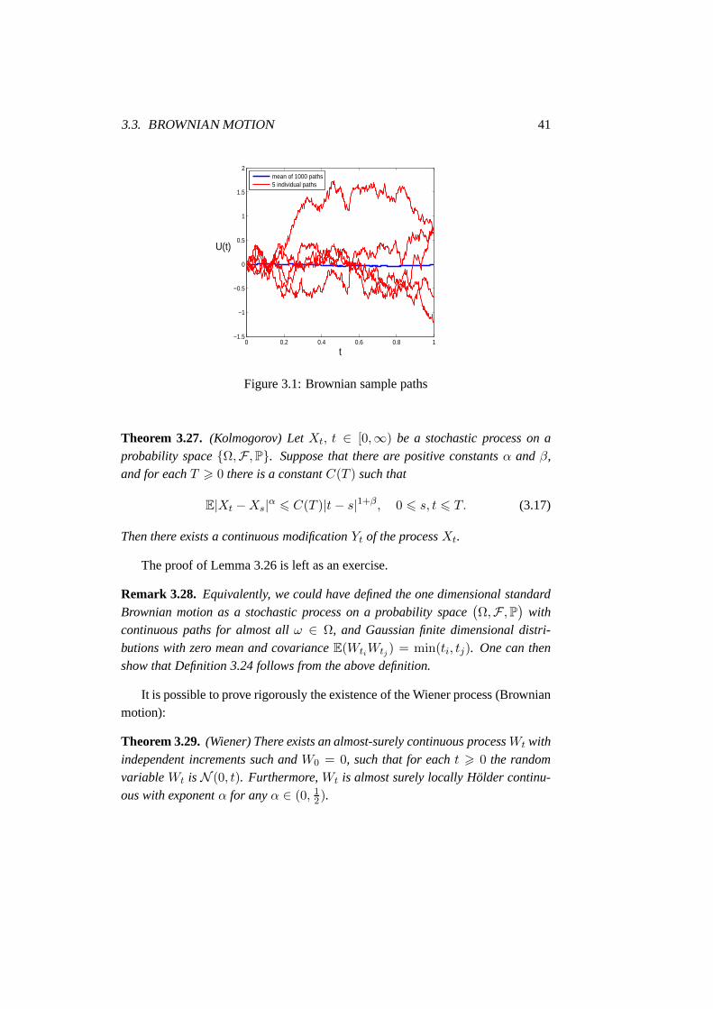
0 0.2 0.4 0.6 0.8 1−1.5
−1
−0.5
0
0.5
1
1.5
2
t
U(t)
mean of 1000 paths5 individual paths
Figure 3.1: Brownian sample paths
Theorem 3.27. (Kolmogorov) LetXt, t ∈ [0,∞) be a stochastic process on aprobability spaceΩ,F ,P. Suppose that there are positive constantsα andβ,and for eachT > 0 there is a constantC(T ) such that
E|Xt −Xs|α 6 C(T )|t− s|1+β, 0 6 s, t 6 T. (3.17)
Then there exists a continuous modificationYt of the processXt.
The proof of Lemma 3.26 is left as an exercise.
Remark 3.28. Equivalently, we could have defined the one dimensional standard
Brownian motion as a stochastic process on a probability space(
Ω,F ,P)
withcontinuous paths for almost allω ∈ Ω, and Gaussian finite dimensional distri-butions with zero mean and covarianceE(WtiWtj ) = min(ti, tj). One can thenshow that Definition 3.24 follows from the above definition.
It is possible to prove rigorously the existence of the Wiener process (Brownianmotion):
Theorem 3.29.(Wiener) There exists an almost-surely continuous processWt withindependent increments such andW0 = 0, such that for eacht > 0 the randomvariableWt is N (0, t). Furthermore,Wt is almost surely locally Holder continu-ous with exponentα for anyα ∈ (0, 1
2).
42 CHAPTER 3. BASICS OF THE THEORY OF STOCHASTIC PROCESSES
Notice that Brownian paths are not differentiable.
We can also construct Brownian motion through the limit of anappropriatelyrescaled random walk: letX1, X2, . . . be iid random variables on a probabilityspace(Ω,F ,P) with mean0 and variance1. Define the discrete time stochasticprocessSn with S0 = 0, Sn =
∑
j=1Xj , n > 1. Define now a continuous timestochastic process with continuous paths as the linearly interpolated, appropriatelyrescaled random walk:
W nt =
1√nS[nt] + (nt− [nt])
1√nX[nt]+1,
where [·] denotes the integer part of a number. ThenW nt converges weakly, as
n→ +∞ to a one dimensional standard Brownian motion.
Brownian motion is a Gaussian process. For thed–dimensional Brownian mo-tion, and forI thed× d dimensional identity, we have (see (2.7) and (2.8))
EW (t) = 0 ∀t > 0
and
E
(
(W (t) −W (s)) ⊗ (W (t) −W (s)))
= (t− s)I. (3.18)
Moreover,
E
(
W (t) ⊗W (s))
= min(t, s)I. (3.19)
From the formula for the Gaussian densityg(x, t − s), eqn. (3.16), we immedi-ately conclude thatW (t) −W (s) andW (t+ u) −W (s+ u) have the same pdf.Consequently, Brownian motion has stationary increments.Notice, however, thatBrownian motion itself is not a stationary process. SinceW (t) = W (t) −W (0),the pdf ofW (t) is
g(x, t) =1√2πt
e−x2/2t.
We can easily calculate all moments of the Brownian motion:
E(xn(t)) =1√2πt
∫ +∞
−∞xne−x2/2t dx
=
1.3 . . . (n− 1)tn/2, n even,0, n odd.
Brownian motion is invariant under various transformations in time.

3.3. BROWNIAN MOTION 43
Theorem 3.30. LetWt denote a standard Brownian motion inR. Then,Wt hasthe following properties:
i. (Rescaling). For eachc > 0 defineXt = 1√cW (ct). Then(Xt, t > 0) =
(Wt, t > 0) in law.
ii. (Shifting). For eachc > 0 Wc+t −Wc, t > 0 is a Brownian motion which isindependent ofWu, u ∈ [0, c].
iii. (Time reversal). DefineXt = W1−t−W1, t ∈ [0, 1]. Then(Xt, t ∈ [0, 1]) =
(Wt, t ∈ [0, 1]) in law.
iv. (Inversion). LetXt, t > 0 defined byX0 = 0, Xt = tW (1/t). Then(Xt, t > 0) = (Wt, t > 0) in law.
We emphasize that the equivalence in the above theorem holdsin law and notin a pathwise sense.
Proof. See Exercise 13.
We can also add a drift and change the diffusion coefficient ofthe Brownianmotion: we will define a Brownian motion with driftµ and varianceσ2 as theprocess
Xt = µt+ σWt.
The mean and variance ofXt are
EXt = µt, E(Xt − EXt)2 = σ2t.
Notice thatXt satisfies the equation
dXt = µdt+ σ dWt.
This is the simplest example of astochastic differential equation.We can define the OU process through the Brownian motion via a time change.
Lemma 3.31. LetW (t) be a standard Brownian motion and consider the process
V (t) = e−tW (e2t).
ThenV (t) is a Gaussian stationary process with mean0 and correlation function
R(t) = e−|t|. (3.20)
44 CHAPTER 3. BASICS OF THE THEORY OF STOCHASTIC PROCESSES
For the proof of this result we first need to show that time changed Gaussianprocesses are also Gaussian.
Lemma 3.32. LetX(t) be a Gaussian stochastic process and letY (t) = X(f(t))
wheref(t) is a strictly increasing function. ThenY (t) is also a Gaussian process.
Proof. We need to show that, for all positive integersN and all sequences of timest1, t2, . . . tN the random vector
Y (t1), Y (t2), . . . Y (tN ) (3.21)
is a multivariate Gaussian random variable. Sincef(t) is strictly increasing, it isinvertible and hence, there existsi, i = 1, . . . N such thatsi = f−1(ti). Thus, therandom vector (3.21) can be rewritten as
X(s1), X(s2), . . . X(sN ),
which is Gaussian for allN and all choices of timess1, s2, . . . sN . HenceY (t) isalso Gaussian.
Proof of Lemma 3.31.The fact thatV (t) is mean zero follows immediatelyfrom the fact thatW (t) is mean zero. To show that the correlation function ofV (t)
is given by (3.20), we calculate
E(V (t)V (s)) = e−t−sE(W (e2t)W (e2s)) = e−t−s min(e2t, e2s)
= e−|t−s|.
The Gaussianity of the processV (t) follows from Lemma 3.32 (notice that thetransformation that givesV (t) in terms ofW (t) is invertible and we can writeW (s) = s1/2V (1
2 ln(s))).
3.4 Other Examples of Stochastic Processes
Brownian Bridge Let W (t) be a standard one dimensional Brownian motion.We define the Brownian bridge (from0 to 0) to be the process
Bt = Wt − tW1, t ∈ [0, 1]. (3.22)
Notice thatB0 = B1 = 0. Equivalently, we can define the Brownian bridge to bethe continuous Gaussian processBt : 0 6 t 6 1 such that
EBt = 0, E(BtBs) = min(s, t) − st, s, t ∈ [0, 1]. (3.23)
3.4. OTHER EXAMPLES OF STOCHASTIC PROCESSES 45
Another, equivalent definition of the Brownian bridge is through an appropriatetime change of the Brownian motion:
Bt = (1 − t)W
(
t
1 − t
)
, t ∈ [0, 1). (3.24)
Conversely, we can write the Brownian motion as a time changeof the Brownianbridge:
Wt = (t+ 1)B
(
t
1 + t
)
, t > 0.
Fractional Brownian Motion
Definition 3.33. A (normalized) fractional Brownian motionWHt , t > 0 with
Hurst parameterH ∈ (0, 1) is a centered Gaussian process with continuous sam-ple paths whose covariance is given by
E(WHt WH
s ) =1
2
(
s2H + t2H − |t− s|2H)
. (3.25)
Proposition 3.34. Fractional Brownian motion has the following properties.
i. WhenH = 12 , W
1
2
t becomes the standard Brownian motion.
ii. WH0 = 0, EWH
t = 0, E(WHt )2 = |t|2H , t > 0.
iii. It has stationary increments,E(WHt −WH
s )2 = |t− s|2H .
iv. It has the following self similarity property
(WHαt , t > 0) = (αHWH
t , t > 0), α > 0, (3.26)
where the equivalence is in law.
Proof. See Exercise 19.
The Poisson Process
Definition 3.35. The Poisson process with intensityλ, denoted byN(t), is aninteger-valued, continuous time, stochastic process withindependent incrementssatisfying
P[(N(t) −N(s)) = k] =e−λ(t−s)
(
λ(t− s))k
k!, t > s > 0, k ∈ N.
The Poisson process does not have a continuous modification.See Exercise 20.
46 CHAPTER 3. BASICS OF THE THEORY OF STOCHASTIC PROCESSES
3.5 The Karhunen-Loeve Expansion
Let f ∈ L2(Ω) whereΩ is a subset ofRd and leten∞n=1 be an orthonormal basisin L2(Ω). Then, it is well known thatf can be written as a series expansion:
f =∞∑
n=1
fnen,
where
fn =
∫
Ωf(x)en(x) dx.
The convergence is inL2(Ω):
limN→∞
∥
∥
∥
∥
∥
f(x) −N∑
n=1
fnen(x)
∥
∥
∥
∥
∥
L2(Ω)
= 0.
It turns out that we can obtain a similar expansion for anL2 mean zero processwhich is continuous in theL2 sense:
EX2t < +∞, EXt = 0, lim
h→0E|Xt+h −Xt|2 = 0. (3.27)
For simplicity we will takeT = [0, 1]. LetR(t, s) = E(XtXs) be the autocorrela-tion function. Notice that from (3.27) it follows thatR(t, s) is continuous in bothtands (exercise 21).
Let us assume an expansion of the form
Xt(ω) =∞∑
n=1
ξn(ω)en(t), t ∈ [0, 1] (3.28)
whereen∞n=1 is an orthonormal basis inL2(0, 1). The random variablesξn arecalculated as
∫ 1
0Xtek(t) dt =
∫ 1
0
∞∑
n=1
ξnen(t)ek(t) dt
=∞∑
n=1
ξnδnk = ξk,
where we assumed that we can interchange the summation and integration. Wewill assume that these random variables are orthogonal:
E(ξnξm) = λnδnm,
3.5. THE KARHUNEN-LOEVE EXPANSION 47
whereλn∞n=1 are positive numbers that will be determined later.Assuming that an expansion of the form (3.28) exists, we can calculate
R(t, s) = E(XtXs) = E
( ∞∑
k=1
∞∑
ℓ=1
ξkek(t)ξℓeℓ(s)
)
=∞∑
k=1
∞∑
ℓ=1
E (ξkξℓ) ek(t)eℓ(s)
=
∞∑
k=1
λkek(t)ek(s).
Consequently, in order to the expansion (3.28) to be valid weneed
R(t, s) =
∞∑
k=1
λkek(t)ek(s). (3.29)
From equation (3.29) it follows that
∫ 1
0R(t, s)en(s) ds =
∫ 1
0
∞∑
k=1
λkek(t)ek(s)en(s) ds
=
∞∑
k=1
λkek(t)
∫ 1
0ek(s)en(s) ds
=
∞∑
k=1
λkek(t)δkn
= λnen(t).
Hence, in order for the expansion (3.28) to be valid,λn, en(t)∞n=1 have to bethe eigenvalues and eigenfunctions of the integral operator whose kernel is thecorrelation function ofXt:
∫ 1
0R(t, s)en(s) ds = λnen(t). (3.30)
Hence, in order to prove the expansion (3.28) we need to studythe eigenvalueproblem for the integral operatorR : L2[0, 1] 7→ L2[0, 1]. It easy to check thatthis operator is self-adjoint ((Rf, h) = (f,Rh) for all f, h ∈ L2(0, 1)) and non-negative (Rf, f > 0 for all f ∈ L2(0, 1)). Hence, all its eigenvalues are realand nonnegative. Furthermore, it is a compact operator (ifφn∞n=1 is a bounded
48 CHAPTER 3. BASICS OF THE THEORY OF STOCHASTIC PROCESSES
sequence inL2(0, 1), thenRφn∞n=1 has a convergent subsequence). The spec-tral theorem for compact, self-adjoint operators implies that R has a countablesequence of eigenvalues tending to0. Furthermore, for everyf ∈ L2(0, 1) we canwrite
f = f0 +∞∑
n=1
fnen(t),
whereRf0 = 0, en(t) are the eigenfunctions ofR corresponding to nonzeroeigenvalues and the convergence is inL2. Finally, Mercer’s Theorem states thatfor R(t, s) continuous on[0, 1] × [0, 1], the expansion (3.29) is valid, where theseries converges absolutely and uniformly.
Now we are ready to prove (3.28).
Theorem 3.36. (Karhunen-Loeve). LetXt, t ∈ [0, 1] be anL2 process withzero mean and continuous correlation functionR(t, s). Letλn, en(t)∞n=1 be theeigenvalues and eigenfunctions of the operatorR defined in(3.36). Then
Xt =∞∑
n=1
ξnen(t), t ∈ [0, 1], (3.31)
where
ξn =
∫ 1
0Xten(t) dt, Eξn = 0, E(ξnξm) = λδnm. (3.32)
The series converges inL2 toX(t), uniformly int.
Proof. The fact thatEξn = 0 follows from the fact thatXt is mean zero. Theorthogonality of the random variablesξn∞n=1 follows from the orthogonality ofthe eigenfunctions ofR:
E(ξnξm) = E
∫ 1
0
∫ 1
0XtXsen(t)em(s) dtds
=
∫ 1
0
∫ 1
0R(t, s)en(t)em(s) dsdt
= λn
∫ 1
0en(s)em(s) ds
= λnδnm.
3.5. THE KARHUNEN-LOEVE EXPANSION 49
Consider now the partial sumSN =∑N
n=1 ξnen(t).
E|Xt − SN |2 = EX2t + ES2
N − 2E(XtSN )
= R(t, t) + E
N∑
k,ℓ=1
ξkξℓek(t)eℓ(t) − 2E
(
Xt
N∑
n=1
ξnen(t)
)
= R(t, t) +
N∑
k=1
λk|ek(t)|2 − 2E
N∑
k=1
∫ 1
0XtXsek(s)ek(t) ds
= R(t, t) −N∑
k=1
λk|ek(t)|2 → 0,
by Mercer’s theorem.
Remark 3.37. Let Xt be a Gaussian second order process with continuous co-varianceR(t, s). Then the random variablesξk∞k=1 are Gaussian, since theyare defined through the time integral of a Gaussian processes. Furthermore, sincethey are Gaussian and orthogonal, they are also independent. Hence, for Gaussianprocesses the Karhunen-Loeve expansion becomes:
Xt =
+∞∑
k=1
√
λkξkek(t), (3.33)
whereξk∞k=1 are independentN (0, 1) random variables.
Example 3.38.The Karhunen-Loeve Expansion for Brownian Motion. The corre-lation function of Brownian motion isR(t, s) = min(t, s). The eigenvalue problemRψn = λnψn becomes
∫ 1
0min(t, s)ψn(s) ds = λnψn(t).
Let us assume thatλn > 0 (it is easy to check that0 is not an eigenvalue). Uponsettingt = 0 we obtainψn(0) = 0. The eigenvalue problem can be rewritten inthe form
∫ t
0sψn(s) ds+ t
∫ 1
tψn(s) ds = λnψn(t).
We differentiate this equation once:∫ 1
tψn(s) ds = λnψ
′n(t).
50 CHAPTER 3. BASICS OF THE THEORY OF STOCHASTIC PROCESSES
We sett = 1 in this equation to obtain the second boundary conditionψ′n(1) = 0.
A second differentiation yields;
−ψn(t) = λnψ′′n(t),
where primes denote differentiation with respect tot. Thus, in order to calcu-late the eigenvalues and eigenfunctions of the integral operator whose kernel isthe covariance function of Brownian motion, we need to solvethe Sturm-Liouvilleproblem
−ψn(t) = λnψ′′n(t), ψ(0) = ψ′(1) = 0.
It is easy to check that the eigenvalues and (normalized) eigenfunctions are
ψn(t) =√
2 sin
(
1
2(2n− 1)πt
)
, λn =
(
2
(2n− 1)π
)2
.
Thus, the Karhunen-Loeve expansion of Brownian motion on[0, 1] is
Wt =√
2
∞∑
n=1
ξn2
(2n − 1)πsin
(
1
2(2n− 1)πt
)
. (3.34)
We can use the KL expansion in order to study theL2-regularity of stochas-tic processes. First, letR be a compact, symmetric positive definite operator onL2(0, 1) with eigenvalues and normalized eigenfunctionsλk, ek(x)+∞
k=1 and con-sider a functionf ∈ L2(0, 1) with
∫ 10 f(s) ds = 0. We can define the one parame-
ter family of Hilbert spacesHα through the norm
‖f‖2α = ‖R−αf‖2
L2 =∑
k
|fk|2λ−α.
The inner product can be obtained through polarization. This norm enables us tomeasure the regularity of the functionf(t).3 LetXt be a mean zero second order(i.e. with finite second moment) process with continuous autocorrelation function.Define the spaceHα := L2((Ω, P ),Hα(0, 1)) with (semi)norm
‖Xt‖2α = E‖Xt‖2
Hα =∑
k
|λk|1−α. (3.35)
Notice that the regularity of the stochastic processXt depends on the decay of theeigenvalues of the integral operatorR· :=
∫ 10 R(t, s) · ds.
3Think of R as being the inverse of the Laplacian with periodic boundaryconditions. In this caseH
α coincides with the standard fractional Sobolev space.
3.6. DISCUSSION AND BIBLIOGRAPHY 51
As an example, consider theL2-regularity of Brownian motion. From Exam-ple 3.38 we know thatλk ∼ k−2. Consequently, from (3.35) we get that, in orderfor Wt to be an element of the spaceHα, we need that
∑
k
|λk|−2(1−α) < +∞,
from which we obtain thatα < 1/2. This is consistent with the Holder continuityof Brownian motion from Theorem 3.29.4
3.6 Discussion and Bibliography
The Ornstein-Uhlenbeck process was introduced by Ornsteinand Uhlenbeck in1930 as a model for the velocity of a Brownian particle [25].
The kind of analysis presented in Section 3.2.3 was initiated by G.I. Taylorin [24]. The proof of Bochner’s theorem 3.16 can be found in [14], where addi-tional material on stationary processes can be found. See also [11].
The spectral theorem for compact, self-adjoint operators which was neededin the proof of the Karhunen-Loeve theorem can be found in [21]. The Karhunen-Loeve expansion is also valid for random fields. See [22] and the reference therein.
3.7 Exercises
1. Let Y0, Y1, . . . be a sequence of independent, identically distributed randomvariables and consider the stochastic processXn = Yn.
(a) Show thatXn is a strictly stationary process.
(b) Assume thatEY0 = µ < +∞ andEY 20 = sigma2 < +∞. Show that
limN→+∞
E
∣
∣
∣
∣
∣
∣
1
N
N−1∑
j=0
Xj − µ
∣
∣
∣
∣
∣
∣
= 0.
(c) Letf be such thatEf2(Y0) < +∞. Show that
limN→+∞
E
∣
∣
∣
∣
∣
∣
1
N
N−1∑
j=0
f(Xj) − f(Y0)
∣
∣
∣
∣
∣
∣
= 0.
4Notice, however, that Wiener’s theorem refers to a.s. Holder continuity, whereas the calculationpresented in this section is aboutL
2-continuity.
52 CHAPTER 3. BASICS OF THE THEORY OF STOCHASTIC PROCESSES
2. LetZ be a random variable and define the stochastic processXn = Z, n =
0, 1, 2, . . . . Show thatXn is a strictly stationary process.
3. LetA0, A1, . . . Am andB0, B1, . . . Bm be uncorrelated random variables withmean zero and variancesEA2
i = σ2i , EB2
i = σ2i , i = 1, . . . m. Letω0, ω1, . . . ωm ∈
[0, π] be distinct frequencies and define, forn = 0,±1,±2, . . . , the stochasticprocess
Xn =
m∑
k=0
(
Ak cos(nωk) +Bk sin(nωk))
.
Calculate the mean and the covariance ofXn. Show that it is a weakly stationaryprocess.
4. Let ξn : n = 0,±1,±2, . . . be uncorrelated random variables withEξn =
µ, E(ξn − µ)2 = σ2, n = 0,±1,±2, . . . . Let a1, a2, . . . be arbitrary realnumbers and consider the stochastic process
Xn = a1ξn + a2ξn−1 + . . . amξn−m+1.
(a) Calculate the mean, variance and the covariance function of Xn. Showthat it is a weakly stationary process.
(b) Setak = 1/√m for k = 1, . . . m. Calculate the covariance function and
study the casesm = 1 andm→ +∞.
5. LetW (t) be a standard one dimensional Brownian motion. Calculate the fol-lowing expectations.
(a) EeiW (t).
(b) Eei(W (t)+W (s)), t, s,∈ (0,+∞).
(c) E(∑n
i=1 ciW (ti))2, whereci ∈ R, i = 1, . . . n and ti ∈ (0,+∞), i =
1, . . . n.
(d) Ee
[
i(
Pni=1
ciW (ti))]
, whereci ∈ R, i = 1, . . . n andti ∈ (0,+∞), i =
1, . . . n.
6. LetWt be a standard one dimensional Brownian motion and define
Bt = Wt − tW1, t ∈ [0, 1].
3.7. EXERCISES 53
(a) Show thatBt is a Gaussian process with
EBt = 0, E(BtBs) = min(t, s) − ts.
(b) Show that, fort ∈ [0, 1) an equivalent definition ofBt is through theformula
Bt = (1 − t)W
(
t
1 − t
)
.
(c) Calculate the distribution function ofBt.
7. Let Xt be a mean-zero second order stationary process with autocorrelationfunction
R(t) =
N∑
j=1
λ2j
αje−αj |t|,
whereαj , λjNj=1 are positive real numbers.
(a) Calculate the spectral density and the correlaction time of this process.
(b) Show that the assumptions of Theorem 3.21 are satisfied and use the argu-ment presented in Section 3.2.3 (i.e. the Green-Kubo formula) to calculatethe diffusion coefficient of the processZt =
∫ t0 Xs ds.
(c) Under what assumptions on the coefficientsαj , λjNj=1 can you study
the above questions in the limitN → +∞?
8. Prove Lemma 3.20.
9. Let a1, . . . an ands1, . . . sn be positive real numbers. Calculate the mean andvariance of the random variable
X =n∑
i=1
aiW (si).
10. LetW (t) be the standard one-dimensional Brownian motion and letσ, s1, s2 >
0. Calculate
(a) EeσW (t).
(b) E(
sin(σW (s1)) sin(σW (s2)))
.
54 CHAPTER 3. BASICS OF THE THEORY OF STOCHASTIC PROCESSES
11. LetWt be a one dimensional Brownian motion and letµ, σ > 0 and define
St = etµ+σWt .
(a) Calculate the mean and the variance ofSt.
(b) Calculate the probability density function ofSt.
12. Use Theorem 3.27 to prove Lemma 3.26.
13. Prove Theorem 3.30.
14. Use Lemma 3.31 to calculate the distribution function ofthe stationary Ornstein-Uhlenbeck process.
15. Calculate the mean and the correlation function of the integral of a standardBrownian motion
Yt =
∫ t
0Ws ds.
16. Show that the process
Yt =
∫ t+1
t(Ws −Wt) ds, t ∈ R,
is second order stationary.
17. LetVt = e−tW (e2t) be the stationary Ornstein-Uhlenbeck process. Give thedefinition and study the main properties of the Ornstein-Uhlenbeck bridge.
18. The autocorrelation function of the velocityY (t) a Brownian particle movingin a harmonic potentialV (x) = 1
2ω20x
2 is
R(t) = e−γ|t|(
cos(δ|t|) − 1
δsin(δ|t|)
)
,
whereγ is the friction coefficient andδ =√
ω20 − γ2.
(a) Calculate the spectral density ofY (t).
(b) Calculate the mean square displacementE(X(t))2 of the position of theBrownian particleX(t) =
∫ t0 Y (s) ds. Study the limitt→ +∞.
19. Show the scaling property (3.26) of the fractional Brownian motion.
3.7. EXERCISES 55
20. Use Theorem (3.27) to show that there does not exist a continuous modificationof the Poisson process.
21. Show that the correlation function of a processXt satisfying (3.27) is continu-ous in botht ands.
22. LetXt be a stochastic process satisfying (3.27) andR(t, s) its correlation func-tion. Show that the integral operatorR : L2[0, 1] 7→ L2[0, 1]
Rf :=
∫ 1
0R(t, s)f(s) ds (3.36)
is self-adjoint and nonnegative. Show that all of its eigenvalues are real andnonnegative. Show that eigenfunctions corresponding to different eigenvaluesare orthogonal.
23. LetH be a Hilbert space. An operatorR : H → H is said to be Hilbert–Schmidt if there exists a complete orthonormal sequenceφn∞n=1 in H suchthat ∞
∑
n=1
‖Ren‖2 <∞.
LetR : L2[0, 1] 7→ L2[0, 1] be the operator defined in (3.36) withR(t, s) beingcontinuous both int ands. Show that it is a Hilbert-Schmidt operator.
24. LetXt a mean zero second order stationary process defined in the interval[0, T ]
with continuous covarianceR(t) and letλn+∞n=1 be the eigenvalues of the
covariance operator. Show that
∞∑
n=1
λn = T R(0).
25. Calculate the Karhunen-Loeve expansion for a second order stochastic processwith correlation functionR(t, s) = ts.
26. Calculate the Karhunen-Loeve expansion of the Brownianbridge on[0, 1].
27. LetXt, t ∈ [0, T ] be a second order process with continuous covariance andKarhunen-Loeve expansion
Xt =
∞∑
k=1
ξkek(t).
56 CHAPTER 3. BASICS OF THE THEORY OF STOCHASTIC PROCESSES
Define the processY (t) = f(t)Xτ(t), t ∈ [0, S],
wheref(t) is a continuous function andτ(t) a continuous, nondecreasing func-tion with τ(0) = 0, τ(S) = T . Find the Karhunen-Loeve expansion ofY (t),in an appropriate weightedL2 space, in terms of the KL expansion ofXt. Usethis in order to calculate the KL expansion of the Ornstein-Uhlenbeck process.
28. Calculate the Karhunen-Loeve expansion of a centered Gaussian stochastic pro-cess with covariance functionR(s, t) = cos(2π(t− s)).
29. Use the Karhunen-Loeve expansion to generate paths of the
(a) Brownian motion on[0, 1].
(b) Brownian bridge on[0, 1].
(c) Ornstein-Uhlenbeck on[0, 1].
Study computationally the convergence of the KL expansion for these pro-cesses. How many terms do you need to keep in the KL expansion in orderto calculate accurate statistics of these processes?

Index
autocorrelation function, 32
Banach space, 16Birkhoff ergodic theorem, 31Bochner theorem, 35Brownian motion, 39Brownian motion
scaling and symmetry properties, 43
central limit theorem, 24characteristic function
of a random variable, 18conditional expectation, 18conditional probability, 12correlation coefficient, 17covariance function, 32
equationFokker–Planck, 2
Fokker–Planck equation, 2fractional Brownian motion, 45
Gaussian stochastic process, 30generating function, 26Green-Kubo formula, 39
Karhunen-Loeve Expansion, 46Karhunen-Loeve Expansion
for Brownian Motion, 49
law
of a random variable, 13law of large numbers
strong, 24law of total probability, 12
Mercer theorem, 48
operatorHilbert–Schmidt, 55
Ornstein-Uhlenbeck process, 36
Poisson process, 45probability density function
of a random variable, 14
random variable, 12random variable
Gaussian, 17uncorrelated, 17
reduced distribution function, 16
sample path, 30sample space, 9spectral density, 35spectral measure, 35stationary process, 31stationary process
second order stationary, 32strictly stationary, 31wide sense stationary, 32
stochastic differential equation, 2, 43
57
58 INDEX
stochastic processdefinition, 29finite dimensional distributions, 30Gaussian, 30sample paths, 30second-order stationary, 32stationary, 31equivalent, 30
stochastic processesstrictly stationary, 31
theoremBochner, 35Mercer, 48
transport coefficient, 39
Wiener process, 40
Bibliography
[1] R. Balescu.Statistical dynamics. Matter out of equilibrium. Imperial CollegePress, London, 1997.
[2] L. Breiman.Probability, volume 7 ofClassics in Applied Mathematics. Soci-ety for Industrial and Applied Mathematics (SIAM), Philadelphia, PA, 1992.Corrected reprint of the 1968 original.
[3] S. Chandrasekhar. Stochastic problems in physics and astronomy. Rev. Mod.Phys., 15(1):1–89, Jan 1943.
[4] A.J. Chorin and O.H. Hald.Stochastic tools in mathematics and science,volume 1 ofSurveys and Tutorials in the Applied Mathematical Sciences.Springer, New York, 2006.
[5] J. L. Doob. The Brownian movement and stochastic equations. Ann. of Math.(2), 43:351–369, 1942.
[6] N. Wax (editor).Selected Papers on Noise and Stochastic Processes. Dover,New York, 1954.
[7] A. Einstein. Investigations on the theory of the Brownian movement. DoverPublications Inc., New York, 1956. Edited with notes by R. F¨urth, Translatedby A. D. Cowper.
[8] W. Feller. An introduction to probability theory and its applications. Vol. I.Third edition. John Wiley & Sons Inc., New York, 1968.
[9] W. Feller. An introduction to probability theory and its applications. Vol. II.Second edition. John Wiley & Sons Inc., New York, 1971.
59
60 BIBLIOGRAPHY
[10] J. Jacod and A.N. Shiryaev.Limit theorems for stochastic processes, vol-ume 288 ofGrundlehren der Mathematischen Wissenschaften [FundamentalPrinciples of Mathematical Sciences]. Springer-Verlag, Berlin, 2003.
[11] S. Karlin and H.M. Taylor.A first course in stochastic processes. AcademicPress [A subsidiary of Harcourt Brace Jovanovich, Publishers], New York-London, 1975.
[12] L. B. Koralov and Y. G. Sinai.Theory of probability and random processes.Universitext. Springer, Berlin, second edition, 2007.
[13] H. A. Kramers. Brownian motion in a field of force and the diffusion modelof chemical reactions.Physica, 7:284–304, 1940.
[14] N. V. Krylov. Introduction to the theory of diffusion processes, volume 142 ofTranslations of Mathematical Monographs. American Mathematical Society,Providence, RI, 1995.
[15] P. D. Lax.Linear algebra and its applications. Pure and Applied Mathematics(Hoboken). Wiley-Interscience [John Wiley & Sons], Hoboken, NJ, secondedition, 2007.
[16] M. Loeve. Probability theory. I. Springer-Verlag, New York, fourth edition,1977. Graduate Texts in Mathematics, Vol. 45.
[17] M. Loeve. Probability theory. II. Springer-Verlag, New York, fourth edition,1978. Graduate Texts in Mathematics, Vol. 46.
[18] R.M. Mazo. Brownian motion, volume 112 ofInternational Series of Mono-graphs on Physics. Oxford University Press, New York, 2002.
[19] E. Nelson. Dynamical theories of Brownian motion. Princeton UniversityPress, Princeton, N.J., 1967.
[20] G. Da Prato and J. Zabczyk.Stochastic Equations in Infinite Dimensions,volume 44 ofEncyclopedia of Mathematics and its Applications. CambridgeUniversity Press, 1992.
[21] Frigyes Riesz and Bela Sz.-Nagy.Functional analysis. Dover PublicationsInc., New York, 1990. Translated from the second French edition by Leo F.Boron, Reprint of the 1955 original.

BIBLIOGRAPHY 61
[22] C. Schwab and R.A. Todor. Karhunen-Loeve approximation of random fieldsby generalized fast multipole methods.J. Comput. Phys., 217(1):100–122,2006.
[23] D.W. Stroock. Probability theory, an analytic view. Cambridge UniversityPress, Cambridge, 1993.
[24] G. I. Taylor. Diffusion by continuous movements.London Math. Soc.,20:196, 1921.
[25] G. E. Uhlenbeck and L. S. Ornstein. On the theory of the Brownian motion.Phys. Rev., 36(5):823–841, Sep 1930.