1

Stochastic Modeling and Direct Simulation of the

Diffusion Media for Polymer Electrolyte Fuel Cells

Yun Wang* and Xuhui Feng

Renewable Energy Resources Lab (RERL) and National Fuel Cell Research Center

Department of Mechanical and Aerospace Engineering

The University of California, Irvine, CA 92697-3975, USA

Ralf Thiedmann and Volker Schmidt

Institute of Stochastics

Ulm University, 89069 Ulm, Germany

Werner Lehnert

Forschungszentrum Jülich GmbH, 52425 Jülich, Germany

A final manuscript submitted to

International J of Heat and Mass Transfer

As a Research Paper

Oct. 2009

*Author to whom correspondence should be addressed:

Email: yunw@uci.edu; phone: 949-824-6004; fax: 949-824-8585

2

Abstract This paper combines the stochastic-model-based reconstruction of the gas diffusion layer

(GDL) of polymer electrolyte fuel cells (PEFCs) and direct simulation to investigate the

pore-level transport within GDLs. The carbon-paper-based GDL is modeled as a stack of

thin sections with each section described by planar 2-dimensional random line

tessellations which are further dilated to three dimensions. The reconstruction is based on

given GDL data provided by scanning electron microscopy (SEM) images. With the

constructed GDL, we further introduce the direct simulation of the coupled transport

processes inside the GDL. The simulation considers the gas flow and species transport in

the void space, electronic current conduction in the solid, and heat transfer in both

phases. Results indicate a remarkable distinction in tortuosities of gas diffusion passage

and solid matrix across the GDL with the former ~1.2 and the latter ~13.8. This

difference arises from the synthetic microstructure of GDL, i.e. the lateral alignment

nature of the thin carbon fiber, allowing the solid-phase transport to occur mostly in

lateral direction. Extensive discussion on the tortuosity is also presented. The numerical

tool can be applied to investigate the impact of the GDL microstructure on pore-level

transport and scrutinize the macroscopic approach vastly adopted in current fuel cell

modeling.

Keywords: polymer electrolyte fuel cell, gas diffusion layer, direct simulation, stochastic

modeling

3

Nomenclature

C molar concentration of species k, mol/m3

D species diffusivity, m2/s

F Faraday’s constant, 96,487 C/equivalent

I current density, A/cm2

j transfer current density, A/cm3

K permeability, m2

P pressure, Pa

R universal gas constant, 8.134 J/mol K

T temperature, K

ur velocity vector, m/s

Greeks

α net water flux per proton flux

ρ density, kg/m3

Φ phase potential, V

ε porosity

τrr shear stress, N/m2

σ electronic or ionic conductivity, S/m;

Superscripts and Subscripts

c cathode

D diffusion

g gas phase

GDL gas diffusion layer

4

k species

o gas channel inlet value; reference value

s solid

5

1. Introduction Fuel cells, converting the chemical energy stored in fuels directly and efficiently to

electricity via electrochemical activity, have become the focus of new energy

development due to their noteworthy features of high efficiency and low emissions [1-3].

Among all types of fuel cells, the polymer electrolyte fuel cells (PEFCs), also called

polymer electrolyte membrane (PEM) fuel cells, have captured the public attention for

both mobile and portable applications [4,5].

Among the PEFC components, the gas diffusion layer (GDL) plays an important

role of electronic connection between the bipolar plate with channel-land structure and

the electrode. In addition, the GDL performs the following functions essential to fuel cell

operation: passage for reactant transport and heat/water removal, mechanical support to

the membrane electrode assembly (MEA), and protection of the catalyst layer from

corrosion or erosion caused by flows or other factors [6,7]. Physical processes in GDLs,

in addition to diffusion, include bypass flow induced by in-plane pressure difference

between neighboring channels [8,9], through-plane flow due to mass source/sink by

electrochemical reactions [10,11], heat transfer [12,13], heat pipe phenomena [14], two-

phase flow [14-18], and electron transport [19-21], to list just a few.

The carbon paper is a common GDL material used in PEFCs. It is non-woven

carbon-fiber-based porous media, where carbon fibers are randomly placed and bonded

by binders. Figure 1 shows a picture of carbon papers. Modeling the transport inside

GDLs is an essential part of a fuel cell model due to the vital role of GDLs. Current effort

in modeling is overwhelmingly through the macroscopic description. This approach

assumes a homogenous structure of GDL and therefore defines several effective

6

parameters accounting for micro structural features, e.g. porosity and permeability. These

parameters are also adopted for modeling other GDL materials, e.g. the carbon cloth and

Sigracet GDLs, and set differently according to their structural characteristics.

Transport in the GDL, e.g. water and oxygen diffusion, are closely related to fuel

cell voltage loss, e.g. the mass transport and Ohmic losses. Typically, diffusion

dominates gaseous species transport in GDLs. Convection may be induced by the local

mass sink/source due to the reaction activities in the catalyst layer [11]. The convection

contributes little comparing with the diffusive one in most cases [11,22]. Some special

designs [8,9] are reported, where convection plays an important role. In addition to

species transport, the reaction heat is removed via the GDL, primarily by heat conduction

in the solid matrix. Recently, liquid water transport within GDLs received much attention.

Liquid may block the pore space, hampering reactant supply. Liquid flow in GDLs is

primarily driven by the capillary action. Its macroscopic modeling is commonly based on

the Darcy’s law and the knowledge of the capillary pressure in porous media [18].

Though great efforts have been made to investigate the macroscopic phenomena,

few are proposed to study the pore-level transport within the GDL. The macroscopic

model requires empirical correlations such as the effective coefficients to account for the

porous media property. These correlations can be developed from the pore-level

information obtained from direct modeling/simulation. In addition, the pore-level study

can provide fundamental details regarding interaction between transport and pore

structure, which is beyond the capability of a usual macroscopic model. The direct

simulation is a powerful numerical tool for studying the transport in porous media. Some

also named it the direct numerical simulation (DNS) [23-25]. To distinguish with the

7

terms in the computational fluid dynamics (CFD), e.g. in the turbulent simulation, we

follow Kaviany [26,27] and choose the term of direct simulation for this numerical

technique. The direct simulation requires precisely capturing the GDL morphology.

Several techniques have been applied to acquire synthetic microstructures of GDLs [28-

32]. An important aspect of a suitable GDL-reconstruction model is the possibility of

fitting it to real data. This paper employs the stochastic model of GDLs developed in

[28]. The optimal parameters of the fitted fiber model are gained using 2D projection

images from electron microscopy. Therefore in Ref. [28] proper segmentation algorithms

are applied to obtain the required structural information from these 2D images. This

means that the model is fitted with respect to structural characteristics but not with

respect to physical properties. The direct simulation model based on realizations of this

stochastic GDL approach is further introduced to study the pore-level phenomena. The

fact that the model is fitted to real data using only structural information of real images

allows the unbiased computations of physical parameters as will be done in this paper. A

typical porosity of ~0.78 of GDLs is considered, which is close to the state of GDLs

without compression or the part of the GDL under the channel [32]. We consider a

typical fuel cell operating condition and solve the fluid, species, heat and electron

equations simultaneously within the GDL. Pore-level information is presented and

discussed.

8

2. Stochastic Modeling of GDLs In this section we give a short description of the stochastic multi-layer model for

reconstructing the GDL microstructure that is based on tools from stochastic geometry

[34, 35]. For details regarding this model and its implementation we refer to Ref. [28].

2.1 Modeling of the fiber system

A look at Figure 1 leads to an impression that the carbon fibers of Toray paper can be

approximated by horizontally orientated straight lines (assume negligible curvature)

which are dilated with respect to 3D. This can also be verified through the production

process of the carbon-paper-based GDL, where fibers are disposed “almost” horizontally.

In addition, it is assumed that the fiber system can be seen as a stack of several thin

sections consisting of such horizontally/laterally orientated fibers which are allowed to

interpenetrate. Therefore the fiber system is modeled as a stack of independent and

identically distributed layers, where adjacent layers are just touching each other. Note

that this assumption is a simplification in comparison to the real GDL because the fibers

in one thin section are crossing each other to a small extent, which is neglected in the

model. Here, the fibers within a given thin section are seen as mutually penetrating

cylinders or filaments. In [28] it was shown that despite of these simplifications the

structure of this model and the structure of physically measured 3D data of such GDLs

are very similar. In [36], tortuosity describing characteristics, pore size distributions, and

connectivity properties of the pore space have been computed for the model and also for

real (physically) measured 3D data. The results for the model and the real measured 3D

data are also very close together with respect to such transport relevant properties. So this

model seems to be appropriate for the here considered kind of GDL.

9

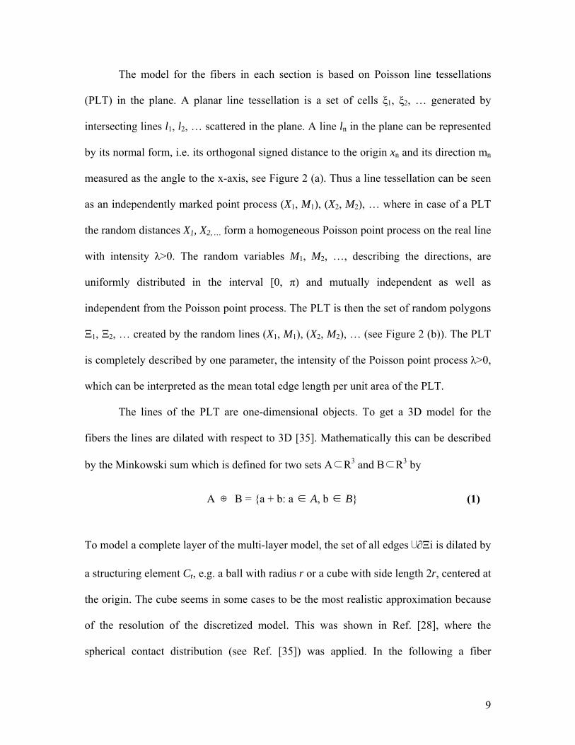
The model for the fibers in each section is based on Poisson line tessellations

(PLT) in the plane. A planar line tessellation is a set of cells ξ1, ξ2, … generated by

intersecting lines l1, l2, … scattered in the plane. A line ln in the plane can be represented

by its normal form, i.e. its orthogonal signed distance to the origin xn and its direction mn

measured as the angle to the x-axis, see Figure 2 (a). Thus a line tessellation can be seen

as an independently marked point process (X1, M1), (X2, M2), … where in case of a PLT

the random distances X1, X2, … form a homogeneous Poisson point process on the real line

with intensity λ>0. The random variables M1, M2, …, describing the directions, are

uniformly distributed in the interval [0, π) and mutually independent as well as

independent from the Poisson point process. The PLT is then the set of random polygons

Ξ1, Ξ2, … created by the random lines (X1, M1), (X2, M2), … (see Figure 2 (b)). The PLT

is completely described by one parameter, the intensity of the Poisson point process λ>0,

which can be interpreted as the mean total edge length per unit area of the PLT.

The lines of the PLT are one-dimensional objects. To get a 3D model for the

fibers the lines are dilated with respect to 3D [35]. Mathematically this can be described

by the Minkowski sum which is defined for two sets A⊂R3 and B⊂R3 by

To model a complete layer of the multi-layer model, the set of all edges ⋃∂Ξi is dilated by

a structuring element Cr, e.g. a ball with radius r or a cube with side length 2r, centered at

the origin. The cube seems in some cases to be the most realistic approximation because

of the resolution of the discretized model. This was shown in Ref. [28], where the

spherical contact distribution (see Ref. [35]) was applied. In the following a fiber

A ⊕ B = {a + b: a ∈ A, b ∈ B} (1)

10

diameter of 7.5 μm and a voxel resolution of 1.5 µm will be considered, following the

real 3D GDL data in [28]. This implies that the fiber diameters have to be modeled by 5

voxels.

The complete multi-layer model consists then of a stack of such dilated PLTs (see

Figure 3), where all layers are assumed to be independent and identically distributed.

Adjacent layers are just touching each other.

2.2 Modeling of the binder

The fibers of the GDL are adhered by means of a binder, which is introduced in the

manufacturing process and can be treated as thin films bounded by fibers. The binder is

modeled by an independent filling of cells, i.e. a cell of the underlying PLT is chosen to

contain binder with probability p ∈ [0,1], see Figure 4.

Structural fitting of the multi-layer model to real data

The considered model for fibers and binder leads to the following formulae for the

volume fractions as described in Ref. [28] and [36], respectively. For notation we use 2r

for describing the side length of the cube which is used to dilate the lines of the PLT, γ

denotes the intensity of the PLT in each layer, and p denotes the probability that a cell is

filled with binder. The expected volume fraction of fibers Vfiber(γ, r) is then given by

The expected volume fraction of binder Vbinder(γ, r, p) is given by

Vfiber(γ, r) = 1 – exp(-2rγ) (2)

Vbinder(γ, r, p) = p exp(-2rγ) (3)

11

Additionally, the relationship ε = 1 – (Vfiber(γ, r) + Vbinder(γ, r, p)) holds, where ε denotes

the (mean) porosity of the considered GDL. In [28], the value γ was estimated from 2D

SEM images for the here considered material where a non-interactive segmentation

algorithm for the detection of the top section has been applied. From the segmented data

the intensity of the PLT was then estimated by 0.025. From 3D images of the same kind

of material, gained by means of synchrotron tomography, in [28] the (mean) porosity ε

was estimated 78%. This value of ε for Toray 090 GDL structures is also known from

literature, see [33]. If these values are plugged in the above given relationship, the

estimated value for p is 0.059 which corresponds to a volume fraction of binder of 4.9%

in the 3D GDL structure. A realization of the complete model can be seen in Figure 5. A

validation of the model with its fitted parameters was done in [28] by the spherical

contact distribution function, see [35]. This characteristic describes the minimum distance

of an arbitrarily chosen point of the pore space to the fiber or binder system, respectively.

Additionally, in [36] it is reported that the model and real measured 3D data are also very

similar with respect to tortuosity describing characteristics, pore size distribution, and

connectivity properties of the pore space.

3. Direct Simulation

3.1 Mathematical modeling

In this section, a small representative GDL is considered for numerical simulation, see

Figure 5. One side surface of the GDL normal to x direction attaches the catalyst layer or

MPL (microscopic layer), while the other in connection to the channel/land region. The

12

physical transports within GDLs are linked to the electrochemical activities in the catalyst

layer, where the following electrochemical reaction takes places:

The reaction consumes oxygen, protons, and electrons, and produces both heat and water.

Among these species, the electron and oxygen supplies rely on the GDL, while heat and

water are removed via both GDL and the electrolyte membrane. In addition, the

electronic current is conducted through the solid matrix of carbon fibers, oxygen and

water transport in the void, while heat transfer occurs in both phases. When excess water

is present, liquid water will emerge, flooding the electrode and GDL. Two-phase (liquid-

gas) transport in fuel cell GDL is a complex phenomenon. It has been widely investigated

in fuel cell literature, mostly in the macroscopic view, and the research is still on-going.

In this paper, our focus is placed on introduction of the combination of the stochastic

modeling and direct simulation; therefore we exclude the liquid transport in the work.

The results can benefit the study of the low-humidity operation and transport

characteristics of the carbon-paper GDL.

3.1.1 Void space

The void space in the GDL is mostly interconnected and allows gas flow. In the direct

simulation of GDL, a fine mesh is applied that is able to distinguish the void and solid. In

the void space, the Navier-Stokes equation can be applied to describe the fluid motion:

O2+4e- +4H+→ 2H2O+heat (4)

13

Note that the quantities in the above are defined at the pore level, therefore macroscopic

characteristics of porosity and permeability no longer appear in the equation.

The void pores also provide passages for species transport. In addition to the

convection induced by the mass flow, diffusion is a major mechanism for water and

oxygen transport. At the pore level of the GDL, the molecular diffusion still dominates

and the transport equations can be unified as:

where the superscript k denotes species and the diffusion coefficient kD depends on the

local condition:

Note that different with the macroscopic model no modifications on the diffusion

coefficient are needed in the direct simulation description. The characteristics of the GDL

structure are already contained in the fine mesh of the direct simulation.

In addition, in the gaseous phase heat transfer occurs and the energy equation

reads

( ) 0)()()(

=⋅∇+∂

∂ ggg

ut

rρρ (5)

( ) τρρ rrrrr

⋅∇+−∇=⎥⎦

⎤⎢⎣

⎡⋅∇+

∂∂ )()()()(

)()(gggg

gg

Puutu (6)

)()( )( kkkgk

CDCut

C∇⋅∇=⋅∇+

∂

∂ r (7)

⎟⎠⎞

⎜⎝⎛

⎟⎠⎞

⎜⎝⎛=

PTDD kk 1

353

2/3

0 (8)

( ) )( )()()()()()()(

)()( gggggp

gg

gp

g TkTuct

Tc ∇⋅∇=⋅∇+∂

∂ rρρ (9)

14

3.1.2 Solid phase

The solid matrix consists of the carbon fibers and binder. The solid matrix is the media

for the electron transport, which can be described by

The above equation is applied to both carbon fibers and binders by setting proper values

of model parameters according to the material properties. In practice the binder material

may vary. We assume identical properties of these two solids in this study.

In both phases, energy equation is applied and can be unified as

where the electronic current flux

3.2 Boundary conditions

Though a 3D GDL is considered, we focus on phenomena in the through-plane (x)

direction, i.e. from the catalyst layer to the channel. The lateral transport will occur due to

the 3D structure of the GDL. In addition, to simplify setting boundary conditions, a

highly-conductive artificial layer is added to the left side of the GDL where each

computational grid contains both solid and gas, and thus allows solid- and gas-phase

transport in each grid, i.e. the conservation equations apply in the region of this layer

without distinguishing the solid and gas phases. Note that due to the conservation

principle applied, the fluxes set on the surface of this pseudo layer, such as heat and

electron, will equal to the ones into/out of the GDL.

3.2.1 GDL surface near the catalyst layer

( ))(0 ss Φ∇⋅∇= σ (10)

s

essss

ps iTk

tTc

σρ 2

)()()()()(

)(r

+∇⋅∇=∂

∂ (11)

)(ssei Φ∇−= σ

r (12)

15

In the catalyst layer, water and heat are produced while oxygen and electrons are

consumed. At the boundary or the interface between the GDL and catalyst layer, fluxes of

oxygen, water, heat and electrons will be induced. The magnitude of the flux is

determined by the reaction rate and transport to the anode side.

Water is added to the cathode by water production and electro-osmatic drag. Both

are proportional to the current density. Part of water will return back to the anode through

back-diffusion. Quantifying the amount of water back diffused requires information of

water level in the anode. In absence of anode water content, the net water transfer

coefficient,α , is frequently used to combine the effects of water back-diffusion and

electro-osmatic drag. Its value is around 0, typically positive. The water flux at this

boundary can then be written as

where F is the Faraday constant and I current density. In fuel cell operation, I may vary

spatially according to local operating condition.

Oxygen is consumed in the cathode. In real case, a small amount of oxygen may

cross the membrane reaching the anode. Neglecting the oxygen cross-over, its flux at the

boundary can be expressed according to its consumption rate

In the cathode, electrons are consumed in the electrochemical reaction in Eq. (4).

The electrolyte membrane typically has an extremely low electronic conductivity,

FICnu

xCD OH

OHOH

2)21(2

22 α+=⎟⎟

⎠

⎞⎜⎜⎝

⎛⋅−

∂∂

−rr (13)

FICnu

xCD O

OO

42

22 −=⎟⎟

⎠

⎞⎜⎜⎝

⎛⋅−

∂∂

−rr (14)

16

therefore most studies only consider electrons from the GDL side. Following the same

assumption, the electronic current at the boundary can then be written as

Mass flows will be induced in the cathode due to the reaction activities. Ref. [11]

identifies three major mechanisms that may contribute the mass source/sink in the gas

phase. Based on their evaluation, electro-osmatic drag and back-diffusion may play an

important role in the induced mass flow. This mass source/sink occurs in the catalyst

layer, which, expressed as rate per volume, can be derived as

where j is the transfer current density and piv

the protonic current flux. j also varies from

place to place including across the catalyst layer [37]. An integral can be taken for the

above equation across the catalyst layer to obtain the surface flux. Again by adopting the

net water transfer coefficient α , the mass flux can be set

The produced heat is taken away from the electrode via the GDL. Most of heat is

generated in the cathode due to the irreversible process. Other heating mechanisms such

as Joule heat arising from the ionic resistance and anode reaction heat also occur in the

MEA. The heat in the MEA is removed via both anode and cathode GDLs. Assuming

half of the heat enters the cathode GDL, the boundary condition for energy equation can

be written as:

Ix

s

s =∂Φ∂

−)(

σ (15)

)(24

)( 2222,22p

dOHOHOOHeffOHm

OHm i

FnM

FjM

FjMCDMS

v⋅∇−−+∇⋅∇= (16)

⎟⎠⎞

⎜⎝⎛ +=⋅− OHH M

FIM

FInu 22

2αρ rr

(17)

17

where oE is defined as Fh

2Δ

− and represents the EMF (electromotive force) that all the

energy from hydrogen/oxygen, the ‘calorific value’, heating value, or enthalpy of

formation, were transformed into electrical energy with water vapor as the reaction

product.

3.2.2 GDL surface near the gas channel

On the right side, GDL connects to the gas channel. In the channel, a stoichiometry

around 1.5-2 is typically used in practice. The air flow is also partially or fully hydrated

prior to injection. The channel velocity is typically ~1 m/s, therefore channel stream is

featured as a low Re laminar flow. The gradients of quantities such as oxygen and water

contents along the channel are small comparing with the in- or through-plane ones,

therefore, we assume constant values at the outer surface of the small part of GDL

considered. The conditions at this boundary are

3.2.3 Void-solid interface

Within the computational domain, we apply equations in each grid according to the phase

it represents. For the void, flow and species equations are applied. At the surface of the

solid matrix, the no-slip and no-flux boundary conditions are set. For electron equation in

IVcellEoTCnuxTk p )(

21

−=⋅−∂∂

− ρrr (18)

0=⎟⎟⎠

⎞⎜⎜⎝

⎛∂∂

Pu

n

r

and

⎟⎟⎟⎟⎟

⎠

⎞

⎜⎜⎜⎜⎜

⎝

⎛

=

⎟⎟⎟⎟⎟

⎠

⎞

⎜⎜⎜⎜⎜

⎝

⎛

Φ VcellTC

C

TC

C

cell

chw

chO

s

w

O 2

)(

2

(19)

18

the solid, no-flux condition is applied at the solid surface. As to energy equation,

temperature and heat flux are continuous across the interface.

3.3 Numerical procedures

The construction of the random lines or PLT, respectively, has already been described in

Section 2, where also the filling of the cells with binder can be found. For the numerical

simulations, the realizations of the stochastic multi-layer model are discretized, where a

voxel resolution of 1.5µm is applied. The governing equations, Eqs.(5)-(11), along with

their appropriate boundary conditions, are discretized by the finite volume method, with

SIMPLE (semi-implicit pressure linked equation) algorithm [38]. The SIMPLE algorithm

is to update the pressure and velocity fields from the solution of the pressure correction

equation, solved by algebraic multi-grid (AMG) method. Following the solution of the

flow field, energy, species, and electron equations are solved. Detailed numerical

discretization can be found in Ref. [18]. About ~2 million (140×140×100) uniform

computational cells are used to describe the complex structure of a GDL (0.21×0.21×0.15

mm) and internal transport phenomena. Geometrical parameters and physical properties

are listed in Table 1. In all the numerical simulations to be presented in the next section,

the equation residuals in all are smaller than 10-6 and the values of species (e.g. O2 and

H2O) and energy global imbalances are all less than 0.1%. A typical simulation takes

about 5 hours with ~2000 iterations based on a single personal computer (CPU 3.0GHz

and 3.5 GB RAM).

4. Results and Discussion The GDL is reconstructed by setting the parameter for the fibers as detected from 2D

images and the (mean) porosity as detected from 3D images, see Ref. [28], which is about

19

78%. This level of porosity fits the portion of the GDL under channels where no

compression is imposed on the GDL [33]. The realization of the GDL model is shown in

Fig. 5. A standard operating condition, 0.5 V and 1.0 A/cm2, is considered in the direct

simulation to display the microscopic transport occurring in the GDL.

Figure 6 shows the velocity distributions at three typical locations. It can be seen

that the local velocity can reach ~0.001 m/s caused by the mass addition in the cathode,

mostly velocity is order-of-magnitude smaller, which is consistent with the prediction by

the macroscopic models [11,18]. The carbon fibers are 7.5 μm in diameter, therefore the

flow can easily go around the fibers. However, the binders are typically flat connecting

fibers and have much larger blocking areas than a single fiber, forcing the flow to go

horizontally/laterally. Strong flows are indicated near the interstitial space primarily due

to blockage of the binders. This figure also indicates that the flow is highly non-uniform

due to the stochastic microstructure of the GDL. Despite that local flow may reach 0.003

m/s, the induced convective transport of species is weak comparing with the diffusion as

indicated by the local Peclet number:

In addition, through the average pressure drop one can obtain the through-plane

permeability K of 3.1×10-12 m2 for this part of porous media using the Darcy’s law

1.0<=g

GDL

Du

Peδ (20)

PKu ∇−=μ

r (21)

20

This value is consistent with that used in literature [6, 18, 39] and is slightly lower than

the one calculated from the Carman-Kozeny model primarily due to the role of the binder

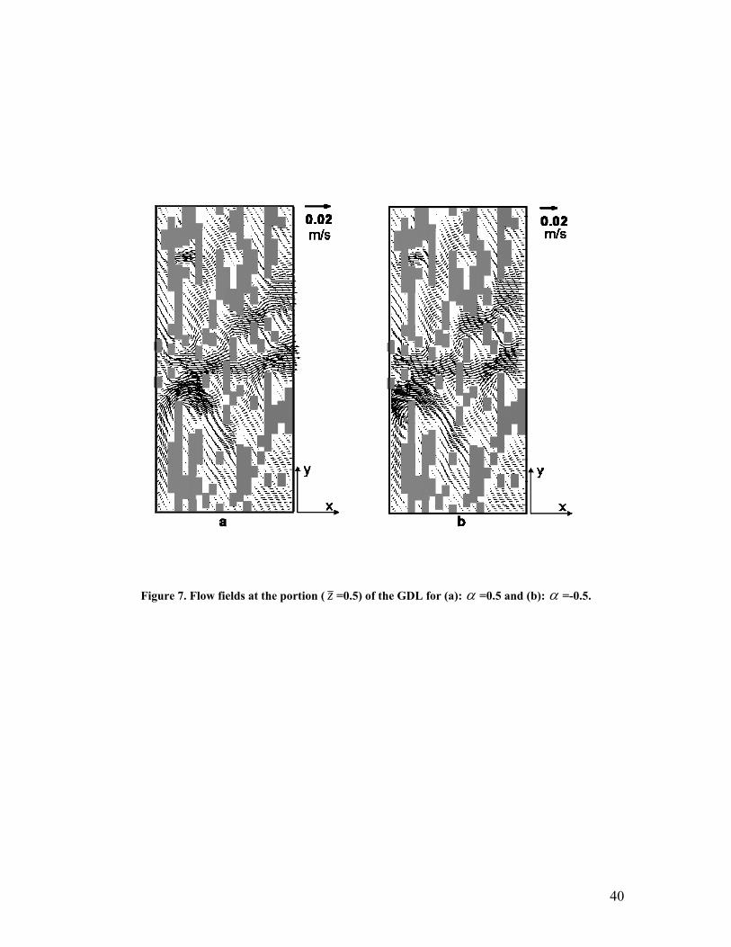
In addition, Figure 7 displays the flow distributions for two different net water

transfer coefficients, α =0.5 and -0.5. At the case of α =0.5, more water mass is added to

the cathode, which may happen at the beginning of the cathode channel when dry

condition is applied in the cathode while the anode is fed with hydrogen at high

humidification. Such an example can be found in Ref. [11]. Due to the increased mass

addition, the magnitude of the induced velocity is significantly increased (over 5 times).

This is also consistent with the conclusion from Ref. [11], which shows that water

activity plays vital role in the mass flow in GDLs. Despite of the flow magnitude, the

flow direction varies little. For the other case, i.e. α =-0.5, the flow reverses with slightly

smaller magnitude in its velocity. The case of a negative α frequently happens for the

counter flow near the cathode outlet and anode inlet, where abundance of produced water

can diffuse to the anode to humidify the dry hydrogen. As mass is withdrawn in the

cathode in this case, the flow will be promoted from the channel to the catalyst layer. As

the flow conductance is determined by the structure of solid matrix which is the same as

the case of the positive α , the flow distribution is similar to Fig. 7 (a) except the

direction.

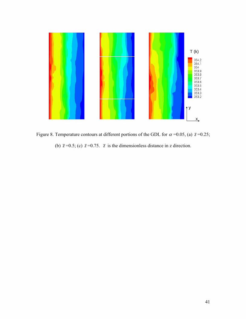
Figure 8 shows the temperature distributions at the three locations of the GDL. As

the thermal conductivity of the solid matrix is several-order-of-magnitude higher than the

air, heat conduction mostly takes place via the randomly placed fibers. Therefore,

22

3

)1(180dK

εε−

= (22)

21

temperature varies in all the directions (x, y, and z directions) as indicated in this figure.

In addition, the temperature variation within the local pore △Td is ~0.2 K. The locations

of carbon fibers are indistinguishable from voids in the contours. This can be explained

by the small pore dimension and negligible convection in the gas phase. Note that the

temperature variation through the GDL, the system level △TL, is only ~1 K, which is

comparable to the pore one △Td, raising the concern of local thermal equilibrium [26].

In addition, the △TL of ~1 K is consistent with our previous prediction and analysis [14,

22].

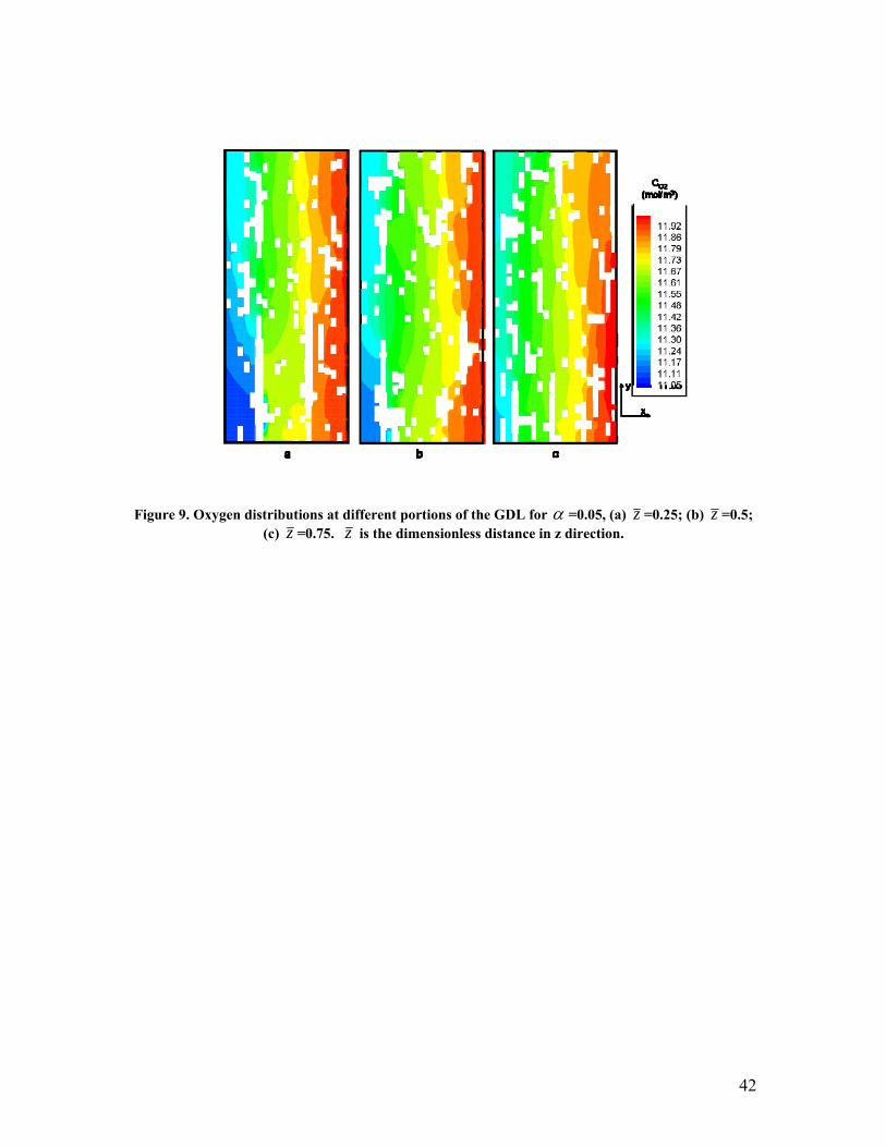
Figure 9 shows the oxygen concentration contours in the void. A small variation

of the oxygen content, ~1 mol/m3, in the through-plane direction is indicated. In addition,

a low oxygen concentration appears in the lower-left corner of Fig. 9 (a), which can be

explained by the local binder blockage, see Fig. 6 (a). Similar contours can be drawn for

water vapor concentration except that the gradients reverse. Also from the structure of the

diffusion media it is evident that the tortuosity of the pore space is much smaller than that

of the solid matrix. This characteristic can be defined as the ratio of the mean effective

path length through the pore space of a porous material and the material thickness [40,

41]. In literature, the tortuosity is usually described as a property of porous media,

defined as the ratio of the actual path length through the pores to the shortest distance

between two points, which lowers in combination with the porosity the effective mass

transport in the medium:

kg

effkg DD

τε

=, (23)

22

The above formula was suggested from the straight-capillary-tube model [42] and

volume averaging [43]. Note that several empirical and analytical relations between the

porosity and the tortuosity exist because in contrast to the porosity the tortuosity can not

be measured directly [44]. Another relationship kg

effkg DD 2

,

τε

= as indicated from the

incline-capillary-tube model [45] is also frequently used [46,47]. Furthermore, it was

shown that the tortuosity may be a function of the temperature, the diffusing species and

the pressure [40, 48]. Besides this, Sharratt and Mann [49] indicated that the tortuosity

may depend on the Thiele modulus if reactions take place inside the porous structures

(which is not the case here). Therefore, the tortuosity as defined in Eq. (23) is not a

unique defined material constant but a parameter which takes into account several effects.

For this reason we would like to name the tortuosity defined above as a “transport based”

tortuosity which takes into account the dynamics of the gas transport. In contrast to this in

Ref. [36] tortuosity is introduced as a (uniquely defined) local material characteristic

which was calculated based on the stochastic model of the GDL. It is also worthy to note

that the “transport-based” tortousity is of significance when dealing with transport

phenomena in the GDL.

Due to the anisotropic GDL material the tortuosity differs in through-plane and

the in-plane directions. We will focus here on the through-plane one. The “transport

based” through-plane tortuosity as calculated with the direct simulation results in an

average value of τ = 1.2. (Notice, that only a small cutout with a small amount of binder

was considered.) This is in good agreement with the calculations presented in Ref. [44].

They also examined Toray material but used a slightly different model for the material.

They simulated the mass transport using the Lattice-Boltzmann technique. In order to

23

determine the tortuosity they computed the flow path length and averaged over the actual

lengths of the flow lines and the flow lines weighted by flux, respectively. Both methods

resulted in values which are very close to each other, the flux weighted tortuosity slightly

lower. As can be seen in Figure 11 of Ref. [44] the calculated tortuosity is about τ = 1.19.

Considering the tortuosity as defined in [36] and calculating its value from

geometric arguments as was done in Ref. [36] results in slightly higher values. The

tortuosities were calculated in three different ways. In the first case the tortuosity was

calculated as the shortest pathways from one side to the other side which results in a

mean value of τ = 1.73. In the other two cases these pathways were weighted with the

capacity (τ = 1.71) and the area (τ = 1.73), respectively.

Only for comparison the well-known Bruggemann equation would result in τ =

1.13 but this relation is unsuitable for describing this kind of porous structure (see e.g.

[34]). Overall it can be said, that all calculated tortuosities are in the same order of

magnitude, the tortuosities calculated from pure geometric arguments show the highest

values. The reason for the deviations is due to the different calculation procedures. The

direct simulation (and the Lattice-Boltzmann simulation) calculate the tortuosity with the

help of mass transport processes in the fibrous structure and are therefore directly linked

to the standard definition of the tortuosity but the information about the structure of the

material under observation is limited.

If calculating the tortuosity from pure geometric arguments using the weighted

graph of the pore structure, one gets information about the structure of the material (e.g.

tortuosity distribution) but the results are not directly linked to mass transport. In order to

24

link the two tortuosities together further examinations are necessary which are beyond the

scope of this paper.

In addition, several studies report utilizing electrical properties in the study of

flow through porous media [50, 51]. The MacMullin number is defined to measure the

ratio of resistance of the porous media saturated with an electrolyte to the bulk resistance

of the same electrolyte [50, 51], i.e. effkg

kg

DD

, for a specific species. This ratio was also

called the formation resistivity factor in an earlier work by Archie [52]. In Eq. 23, the

MacMullin number is implicitly defined as ετ , and its value from the direct simulation is

~1.6 for the carbon paper considered.

Figure 10 shows the oxygen and temperature profiles at the cross line of the mid-

planes in z and x directions for both α =0.05 and 0.5. These two cases indicate similar

flow distribution but with quite different magnitudes. For the oxygen, the concentration

along this line shows a small variation in each case, which is attributed to the diffusion

that dominates the mass transport. The random solid matrix either leads to blockage of

the diffusion or varies local flow, leading to fluctuation of oxygen concentration from

place to place. The case of the higher α shows a lower oxygen profile. This can be

explained by the fact that a higher α induces a stronger flow towards the gas channel,

see Fig. 6 (b) and 7 (a). Note that the convection by the flow is against the direction of

oxygen diffusion for the reaction. Again the difference is small (~0.1 mol/m3) due to the

relatively weak convection force. Fig. 10 (b) presents the temperature profiles, showing

the two are very close with the case of α =0.5 slightly lower. This is due to the fact that

the flow from the electrode delivers thermal energy therefore helps heat removal,

25

however the amount is small and most is still removed by the highly conductive carbon

fiber. Temperature variation near the solid-gas interface is moderate, indicating little heat

is transferred between two phases partly due to the small gas heat capacity. However, the

gas temperature is largely affected by the neighboring carbon fiber due to the small scale

of the pore.

Figure 11 displays the electronic phase potential distributions in the solid matrix

at the three locations. Though the figure shows disconnected solid matrix, the fibers are

connected in the 3D structure. A small but discernible drop of the electronic phase

potential can be observed from the electrode side to the channel. This is because though

the carbon fiber is a good thermal conductor, the highly tortuous nature of the solid

matrix leads to non-negligible ohmic resistance. Similar to oxygen transport in the pore,

electron transport totally relies on the highly tortuous solid matrix. The high tortuosity

arises from the fact that the fibers are arranged in the in-plane direction and the through-

plane conduction only occurs at the joint points of fibers. By applying a similar approach

as Eq. (23) ( ss

effs σ

τεσ )1( −

= ), the tortuosity sτ is 13.8 for the solid matrix. Again from

previous discussion, this tortuosity is referred to the “transport-based” one and may

slightly deviate from the material intrinsic property. Further, the obtained tortuosity is for

the through-plane transport, which may be different with the in-plane one as the carbon

paper is anisotropic. Ref. [6] indicates that the through-plane conductivity is an-order-of-

magnitude lower than the in-plane one. This figure shows that the unique structure of the

carbon paper, the high through-plane tortuosity, may be a major reason for the relatively

lower conductivity in the through-plane direction.

26

5. Conclusions

This paper combined the stochastic modeling for reconstruction of microstructure of

GDLs and direct simulation for study of the mass transport at the pore level. A stochastic

model was applied for the carbon-paper-based GDL, which models the GDL as a stack of

thin sections with each section described by planar 2-dimensional random line

tessellations extended to three dimensions by dilation. The direct simulation was then

introduced to the reconstructed GDL structure to simulate the flow and species transport

in the void, electronic current conduction in the solid matrix, and heat transfer in both

phases. Standard conditions of fuel cells are considered in the simulation. Distributions of

the flow, species concentration, temperature, and electronic phase potential in the GDL

are presented at the pore level. Simulation results indicated that the through-plane

tortuosity of the solid matrix is an-order-of-magnitude larger than the one of the pore

structure. The predicted values of tortuosity and permeability are in good agreement with

the ones in the literature. In addition, diffusion dominates the species transport in the pore

even at high values of net water transfer coefficient. The developed numerical tools can

be applied to investigate the pore-level phenomena within the carbon paper based GDL.

Future study includes investigation of the different realizations of porous materials which

allows a statistical analysis of the numerical simulation results and the influence of the

compression over the GDL on in-plane and through-plane mass transport.

Acknowledgements: This research has been supported by the Faculty Career

Development Award at UCI and the German Federal Ministry for Education and Science

(BMBF) under Grant No. 03SF0324.

27

References

1. M.L. Perry and T.F. Fuller, J. Electrochem. Soc., 149 (2002) S59-67.

2. J. Larminie and A. Dicks, Fuel Cell Systems Explained (2nd Edition), John Wiley

& Sons (2003).

3. C.Y. Wang, Chemical Reviews, 104 (2004) 4727-4765.

4. P. Costamagna and S. Srinivasan, J. Power Sources, 102 (2001) 242-252.

5. P. Costamagna and S. Srinivasan, J. Power Sources, 102 (2001) 253-269.

6. M. Mathias, J. Roth, J. Fleming, and W. Lehnert, “Diffusion Media Materials and

Characterization”, in: W. Vielstich, H. Gasteiger, A. Lamm (Eds.), Handbook of

Fuel Cells: Fundamentals, Technology and Applications, vol .3, John Wiley &

Sons, Ltd, (2003).

7. C.H. Hartnig, L. Jörissen, J. Kerres, W. Lehnert, J. Scholta, Polymer electrolyte

membrane fuel cells (PEMFC) in: Materials for Fuel Cells, Ed. M. Gasik,

Woodhead Publishing Limited, 2008.

8. J.S. Yi and T. V. Nguyen, J. Electrochem. Soc., 146 (1999) 38.

9. Y. Wang and C. Y. Wang, J. Power Sources, 147 (2005) 148.

10. S. Dutta, S. Shimpalee, and J.W. Van Zee, J. Appl. Electrochem., 30 (2000) 135.

11. Y. Wang and C.Y. Wang, J. Electrochem. Soc., 152(2) (2005) A445.

12. S. Mazumder and J.V. Cole, J. Electrochem. Soc., 150 (2003) 1503.

13. J. J. Hwang, J. Electrochem. Soc., 153 (2006) A216.

14. Y. Wang and C.Y. Wang, J. Electrochem. Soc., 153 (2006) A1193

28

15. E. Birgersson, M. Noponen, and M. Vynnycky, J. Electrochem., 152 (2005)

A1021.

16. U. Pasaogullari and C.Y. Wang, J. Electrochem. Soc., 151 (2004) A399.

17. J.-H. Nam and M. Kaviany, Int. J. Heat and Mass Transfer, 46 (2003) 4595.

18. Y. Wang, Journal of Power Sources, 185 (2008) 261–271.

19. D.M. Bernardi and M.W.Verbrugge, J. Electrochem. Soc., 139 (1992) 2477.

20. H. Meng and C. Y. Wang, J. Electrochem. Soc., 151 (2004) A358.

21. H. Meng, J. Power Sources 162 (2006) 426.

22. Y. Wang, J. Electrochem. Soc., 154 (2007) B1041-B1048.

23. P. P. Mukherjee and C. Y. Wang, J. Electrochem. Soc., 153 (2006) A840.

24. M. Piller, G. Schena, M. Nolich, S. Favretto, F. Radaelli and E. Rossi, Transport

in Porous Media, 80, (2009) 57.

25. V. P. Schulz, P. P. Mukherjee, J. Becker, A. Wiegmann, and C. Y. Wang, ECS

Transactions, 3 (2006) 1069.

26. M. Kaviaty, Principles of Heat Transfer in Porous Media, 2nd edition, Springer,

1999.

27. M. Kaviany, Principles of convective heat transfer, Springer, 2nd edition, 2001.

28. R. Thiedmann, F. Fleischer, Ch. Hartnig, W. Lehnert, and V. Schmidt, J.

Electrochem. Soc., 155 (2008) B391-B399.

29. V.P. Schulz, J. Becker, A. Wiegmann, P.P. Mukherjee, and C.-Y. Wang. J.

Electrochem. Soc., 154(4) (2007) B419-B426.

30. G. Inoue, Y. Matsukuma, M. Minemoto. Proceedings of the 2nd European Fuel

Cell Technology and Applications Conference, EFC2007-39024 (2007).

29

31. M. Yoneda, M. Takimoto, S. Koshizuka. ECS Transactions, 11 (2007) 629-635.

32. G. Inoue, T. Yoshimoto, Y. Matsukuma, M. Minemoto. Journal of Power Sources

175 (2008) 145-158.

33. J. T. Gostick, M. W. Fowler, M. A. Ioannidis, M. D. Pritzker, Y. M. Volfkovich,

and A. Sakars, J. Power Sources, 156 (2006) 375-387.

34. R. Schneider and W. Weil, Stochastic and Integral Geometry. Springer, Berlin

(2008).

35. D. Stoyan, W.S. Kendall, and J. Mecke. Stochastic Geometry and its

Applications. 2nd ed. J. Wiley & Sons, Chichester (1995).

36. R. Thiedmann, Ch. Hartnig, I. Manke, V. Schmidt, and W. Lehnert. J.

Electrochem. Soc., 156(11) (2009), B1339 – B1347.

37. Y. Wang and X. Feng, J. Electrochem. Soc., 155(12) (2008) B1289-B1295.

38. S.V. Patankar, Numerical Heat Transfer and Fluid Flow, Hemisphere Publishing

Corp., New York (1980).

39. J.P. Feser, A.K. Prasad and S.G. Advani, J. Power Sources 162 (2006) 1226–

1231.

40. F. Keil, Diffusion und Chemische Reaktionen in der Gas/Feststoff–Katalyse.

Springer, Berlin (1999).

41. L. Shen and Z. Chen, Critical Review of the Impact of Tortuosity on Diffusion.

Chem. Eng. Sci., 62 (2007) 3748–3755.

42. M. R. J. Wyllie and M. B. Spangler, Am. Assoc. Pet. Geol. Bull., 36, 359 (1952).

43. S. Liu and J. H. Masliyah, in Handbook of Porous Media, pp. 81–140, K. Vafai,

Editor, CRC Press, Boca Raton FL (2005).

30

44. Y. S. Wua, L. J. van Vliet, H. W. Frijlink, K. van der Voort Maarschalk,

European Journal of Pharmaceutical Sciences 28 (2006) 433–440.

45. D. Cornell and D. L. Katz, Ind. Eng. Chem., 45, 2145 (1953).

46. K. M. Abraham, Electrochim. Acta, 38, 1233 (1993).R5. K. K. Patel, J. M.

Paulsen, and J. Desilvestro, J. Power Sources, 122, 144 (2003).

47. D. Djian, F. Alloin, S. Martinet, H. Lignier, and J. Y. Sanchez, J. Power Sources,

172, 416 (2007).

48. S.K. Bhatia, Chem. Eng. Sci. 41 (1986) 1311.

49. P.N. Sharratt and R. Mann, Some observations on the variation of tortuosity with

Thiele modulus and pore size distribution. Chemical Engineering Science 42(7)

(1987), 1565–1576.

50. R. B. MacMullin and G. A. Muccini, AIChE J., 2, 393 (1956).

51. M. J. Martinez, S. Shimpalee, and J. W. Van Zee, J.Electrochem. Soc., 156, B80

(2009).

52. G. E. Archie, Trans. Am. Inst. Min., Metall. Pet. Eng., 146, 54 (1942).

31

Table 1. Geometrical, physical, and operating parameters.

Quantity Value

Fiber cross-section dimension, (side length) 7.5 μm

GDL thickness, δ 0.015 mm

Pressures, P 2.0 atm

Porosity of GDLs, ε 0.78

Thermal conductivity of air, )(gk 0.025 W/m K

Thermal conductivity of carbon fibers and binders, )(sk 10 W/m K

Electronic conductivity of carbon fibers, sσ 20000 S/m

Species diffusivity in cathode gas @standard condition, Do,O2/w 3.24/3.89×10-5 m2/s

32

List of the figures

1. Figure 1. Microscope image of carbon paper diffusion media used in PEFCs..... 34

2. Figure 2. a) Construction of a line, b) A cell Ξn of a PLT. ................................... 35

3. Figure 3: Schematic display of the multilayer model: a= one layer, b) two layers,

c) several layers..................................................................................................... 36

4. Figure 4. a) Cells without binder, b) Some cells filled with binder...................... 37

5. Figure 5 (a). A realization of the stochastic model for carbon paper GDL

reconstruction; (b). The solid matrix; (c) Solid matrix cross-section at x =20%;

(d) Solid matrix cross-section at x =80%. ............................................................ 38

6. Figure 6. Flow fields at different portions of the GDL for α =0.05, (a) z =0.25;

(b) z =0.5; (c) z =0.75. z is the dimensionless distance in z direction ranging

from 0 to 1. The gray region denotes the solid with the light gray being the carbon

fibers and the dark the binders. ............................................................................. 39

7. Figure 7. Flow fields at the portion ( z =0.5) of the GDL for (a): α =0.5 and (b): -

0.5.......................................................................................................................... 40

8. Figure 8. Temperature contours at different portions of the GDL for α =0.05, (a)

z =0.25; (b) z =0.5; (c) z =0.75. z is the dimensionless distance in z direction

ranging from 0 to 1. .............................................................................................. 41

9. Figure 9. Oxygen distributions at different portions of the GDL for α =0.05, (a)

z =0.25; (b) z =0.5; (c) z =0.75. z is the dimensionless distance in z direction

ranging from 0 to 1. .............................................................................................. 42

33

10. Figure 10. Distributions of quantities at the cross line of the planes z =0.5 and

5.0=x ; (a). the oxygen concentration; (b) temperature. z and x are the

dimensionless distances in z and x directions, respectively. ................................ 43

11. Figure 11. Electronic phase potential distributions at different portions of the

GDL for α =0.05, (a) z =0.25; (b) z =0.5; (c) z =0.75, where z is the

dimensionless distance in z direction ranging from 0 to 1.................................... 44

34

Figure 1. Microscope images of the carbon paper diffusion media used in PEFCs.

35

Figure 2. a) Construction of a line, b) A cell Ξn of a PLT.

36

Figure 3: Schematic display of the multilayer model: a= one layer, b) two layers, c) several layers.

37

Figure 4. a) Cells without binder, b) Some cells filled with binder.

38

Figure 5 (a). A realization of the stochastic model for carbon paper GDL reconstruction; (b). The solid matrix; (c) Solid matrix cross-section at x =20%; (d) Solid matrix cross-section at x =80%.

39

Figure 6. Flow fields at different portions of the GDL for α =0.05, (a) z =0.25; (b) z =0.5; (c) z =0.75. z is the dimensionless distance in z direction ranging from 0 to 1. The gray region denotes

the solid with the light gray being the carbon fibers and the dark the binders.

40

Figure 7. Flow fields at the portion ( z =0.5) of the GDL for (a): α =0.5 and (b): α =-0.5.

41

x

y

T (k)

x

y

T (k)

Figure 8. Temperature contours at different portions of the GDL for α =0.05, (a) z =0.25;

(b) z =0.5; (c) z =0.75. z is the dimensionless distance in z direction.

42

Figure 9. Oxygen distributions at different portions of the GDL for α =0.05, (a) z =0.25; (b) z =0.5; (c) z =0.75. z is the dimensionless distance in z direction.

43

z0 0.2 0.4 0.6 0.8 1

11.4

11.5

11.6

11.7

11.8

11.9

V2

0 0.2 0.4 0.6 0.8 111.4

11.5

11.6

11.7

11.8

11.9

V2

=0.5

=0.05

αα

Solid matrix location

y

O2

conc

entra

tion

(mol

/m3 )

z0 0.2 0.4 0.6 0.8 1

11.4

11.5

11.6

11.7

11.8

11.9

V2

0 0.2 0.4 0.6 0.8 111.4

11.5

11.6

11.7

11.8

11.9

V2

=0.5

=0.05

αα

Solid matrix location

y

O2

conc

entra

tion

(mol

/m3 )

(a)

0 0.2 0.4 0.6 0.8 1353.2

353.4

353.6

353.8

354

354.2

V3

z0 0.2 0.4 0.6 0.8 1

353.2

353.4

353.6

353.8

354

354.2

V3=0.5=0.05

αα

Solid matrix location

y

Tem

pera

ture

(K)

0 0.2 0.4 0.6 0.8 1353.2

353.4

353.6

353.8

354

354.2

V3

z0 0.2 0.4 0.6 0.8 1

353.2

353.4

353.6

353.8

354

354.2

V3=0.5=0.05

αα

0 0.2 0.4 0.6 0.8 1353.2

353.4

353.6

353.8

354

354.2

V3

z0 0.2 0.4 0.6 0.8 1

353.2

353.4

353.6

353.8

354

354.2

V3=0.5=0.05

αα

Solid matrix location

y

Tem

pera

ture

(K)

(b)

Figure 10. Distributions of quantities at the cross line of the planes z =0.5 and 5.0=x ; (a). the oxygen concentration; (b) temperature. z and x are the dimensionless distances in z and x

directions, respectively.

44

Figure 11. Electronic phase potential distributions at different portions of the GDL for

α =0.05, (a) z =0.25; (b) z =0.5; (c) z =0.75, where z is the dimensionless distance in z

direction ranging from 0 to 1.