stochastic model for detection of signals in noisecornea.berkeley.edu/pubs/195.pdf · stochastic...

1Iaottdsnrmpoken

trtntgepuw

waa

B110 J. Opt. Soc. Am. A/Vol. 26, No. 11 /November 2009 S. A. Klein and D. M. Levi

Stochastic model for detection of signals in noise

Stanley A. Klein* and Dennis M. Levi

School of Optometry, University of California, Berkeley, Berkeley, California 94720, USA*Corresponding author: [email protected]

Received June 19, 2009; revised October 2, 2009; accepted October 5, 2009;posted October 5, 2009 (Doc. ID 113069); published October 30, 2009

Fifty years ago Birdsall, Tanner, and colleagues made rapid progress in developing signal detection theory intoa powerful psychophysical tool. One of their major insights was the utility of adding external noise to the sig-nals of interest. These methods have been enhanced in recent years by the addition of multipass andclassification-image methods for opening up the black box. There remain a number of as yet unresolved issues.In particular, Birdsall developed a theorem that large amounts of external input noise can linearize nonlinearsystems, and Tanner conjectured, with mathematical backup, that what had been previously thought of as anonlinear system could actually be a linear system with uncertainty. Recent findings, both experimental andtheoretical, have validated Birdsall’s theorem and Tanner’s conjecture. However, there have also been experi-mental and theoretical findings with the opposite outcome. In this paper we present new data and simulationsin an attempt to sort out these issues. Our simulations and experiments plus data from others show that Bird-sall’s theorem is quite robust. We argue that uncertainty can serve as an explanation for violations of Birdsall’slinearization by noise and also for reports of stochastic resonance. In addition, we modify present models tobetter handle detection of signals with both noise and pedestal backgrounds. © 2009 Optical Society ofAmerica

OCIS codes: 330.4060, 330.5510.

ag

wbcep

pnllw1nittalc

mp

dpdmpiOe

. INTRODUCTIONt is fitting for this special issue commemorating Birdsallnd Tanner to explore, in depth, the topic of the detectionf signals in noise. “Google” Birdsall and Tanner and seehe richness of the research on this topic in the mid-1950so 1960s at the University of Michigan. Ted Cohn, a stu-ent there in the latter part of that era, edited a book, Vi-ual Detection [1], with a multiplicity of articles by Tan-er, Birdsall, and dozens of others. The articles areemarkable in their depth and sophistication, and itakes one wonder whether much new has been accom-

lished in the past 50 years. The present article will focusn an important contribution from Ted Birdsall that isnown as Birdsall’s theorem, and in the process we willxamine the general topic of modeling the detection of sig-als in both noise and known backgrounds.Birdsall’s theorem has relevance to any study of detec-

ion of signals in noise. A concise statement of the theo-em was given by Lasley and Cohn [2], p. 275: “Accordingo Birdsall’s Theorem, when the variance of any source ofoise prior to the nonlinear transducer is large enough sohat other sources of noise in an experiment can be ne-lected, the resulting d� psychometric function will be lin-ar.” A mathematical derivation of Birdsall’s theorem wasrovided by Lasley and Cohn (Appendix A) [2]. It can benderstood by considering a simple nonlinear systemith external noise:

y�ctest,�ext� = �ctest + �extR1�� + �intR2, �1�

here ctest is the contrast of the test pattern, �ext and �intre the external and internal noise standard deviations,nd R is a Gaussian random number with a mean of zero
i
1084-7529/09/11B110-17/$15.00 © 2

nd unity standard deviation. Three cases can be distin-uished:

Case 1. If �ext is negligible then by the definition of d�e have d�=ctest

� /�int, the ratio of signal strength dividedy noise standard deviation. The astute reader may beonfused by �ext

� and �int having the same units. In futurequations we will be more careful; however, this confusingractice is common.Case 2. If �int is negligible then we are faced with the

roblem of Gaussian noise raised to a power making theoise non-Gaussian. Non-Gaussian noise produces a prob-

em in defining d� that is based on Gaussian noise. Asong as �int is negligible, the Gaussian nature of the noiseould be restored by raising both sides of Eq. (1) to the/� power. The new response variable y1/� has Gaussianoise, so it is the appropriate variable for defining d�, giv-

ng d�=ctest /�ext. This linearization of the dependence onest contrast is Birdsall’s theorem. This value of d� is alsohe value of d� for a generic ideal observer as long as ctestnd �ext are defined in terms of the overlap of the stimu-us with a template matched to the test pattern, as is dis-ussed following Eq. (2).

Case 3. If neither �int nor �ext is negligible, a simple for-ula for d� isn’t possible. This case is the focus of the

resent paper.Dosher and Lu [3] and Lu and Dosher [4,5] report their

ata and data of others where the linearizing effect ex-ected from strong external noise and Birdsall’s theoremoesn’t hold, and they have developed a model based onultiplicative noise consistent with their finding. In this

aper we examine both the experimental and the theoret-cal underpinnings of the Birdsall linearization effect.ur simulations and our experiments plus data from oth-rs show that Birdsall’s theorem is more robust than had

009 Optical Society of America

bt

cntrttcs

cocTna

Tioi

2TtsL

wnounotan��pRq

ismtuttdtatt

L“bbaatwnt

n�spnt(E

Arcl

cttfDh

atp1fiPcvEit

maofdptstp

S. A. Klein and D. M. Levi Vol. 26, No. 11 /November 2009 /J. Opt. Soc. Am. A B111

een expected. We explore how this apparent conflict be-ween different sets of data might be resolved.

We will also consider a related topic of concern to Cohn,alled “stochastic resonance,” whereby small amounts ofoise backgrounds can produce a pedestal effect facilita-ion similar to that of nonrandom backgrounds [6,7]. Ofelevance is Tanner’s finding that the presence of uncer-ainty can mimic a nonlinear transduction. We will arguehat uncertainty can serve as an explanation for the sto-hastic resonance findings and also for violations of Bird-all’s linearization by noise.

Although all of our simulations will be based on a dis-rimination model with multiplicative noise, we will pointut that the same conclusions would apply to a class ofontrast gain control models with no multiplicative noise.he identity between this broad class of multiplicativeoise models and gain control models deflates some of therguments associated with distinguishing the two [8–11].Finally, we will thoroughly examine the Perceptual

emplate Model (PTM) that has the potential for describ-ng both the detection of signals on known pedestals andn unknown noise [3–5]. We modify that model slightly tomprove its performance on known pedestals.

. METHODShe following simple, plausible, stochastic (inclusion ofrial-by-trial noise) model for the response of the visualystem to a test pattern is the PTM used by Dosher andu [3] (Appendix A):

y�ctest,�ext� = �ctest/Ttest + �ext/TextR1�� + �addR2 + �multR3,

�2�

here ctest is the overlap of a template with the originaloisy stimulus and �ext is the standard deviation of thatverlap with multiple samples of the external noise. Wese the notation Ri as in Eq. (1) for different randomumbers on each trial [12]. The first term in Eq. (2) is theutput of a single channel that gets stimulation from theest stimulus plus the external random noise, followed bynonlinear transduction. The last two terms are additiveoise following the nonlinearity with the second term

�addR2� being a fixed additive noise and the final term�multR3� being a noise contribution whose strength de-ends on the stimulus strength of the first term. Becausei can be negative and is raised to a power, we define a

uantity raised to a power to be Q�=sign�Q�abs�Q�� [3].Before discussing the role of the various parameters, it

s useful to specify the performance of the ideal observerpecified by �add=0, �mult=0, with the template beingatched to the image of the test pattern. The matched fil-

er is the ideal template as long as the noise samples arencorrelated (white noise). As was derived in Case 2 ofhe Introduction (Section 1), the d� of the ideal observer ishe ratio of the test strength ctest divided by the standardeviation of the test strength, �ext: dideal� =ctest /�ext. Forhis simple formula it is important that both ctest and �extre measured using a template matched to the test pat-ern. If the ideal observer is modified by using a templatehat differs from the ideal template then d becomes
�
dtemplate� = �ctest/Ttest�/��ext/Text�. �3�

evi and Klein [12] called this near-ideal observer theTemplate Observer” with the nonideal template able toe estimated using classification images [13,14]. Usingoth multipass and classification-image techniques welso showed that the mismatched template accounted forlmost all of the noise that was consistent across repeatedrials. It is useful to note that the conditions for Eq. (3),ith the external input noise dominating other sources ofoise, are precisely the conditions needed for Birdsall’sheorem to produce a linear d� function.

For realistic models the additive and multiplicativeoise standard deviations are given in Eq. (2) by �add andmult. yi (Eq. (2)) can be multiplied by an arbitrary con-tant without changing d�, because d�, the measure ofsychophysical performance, is based on a ratio of the sig-al term and the noise terms. We will follow the conven-ional choice for scaling the parameters by dividing Eq.2) by �add [15] and redefining the various parameters soq. (2) becomes

y�ctest,1,�ext� = �ctest,1/Ttest + �ext/TextR1�� + R2 + �multR3.

�4�

subscript, 1, has been added to ctest for later use to rep-esent one of the intervals of a two-alternative forced-hoice (2AFC) experiment. Each term of Eq. (4) is unit-ess, simplifying its interpretation.

The same formalism can be applied to tasks other thanontrast detection or contrast discrimination (like orien-ation discrimination) by having the single template behe difference of the two stimuli being discriminated. Byocusing on the output of a single template, Lu andosher simplified the specification of the model while stillaving it apply to a wide range of tasks [4].The variables Ttest and Text are model parameters that

re used in data fitting, and �mult that specifies the mul-iplicative noise will be clarified in Eq. (5). Ttest and Textlay the same role as the Lu and Dosher [4] parameters/� and 1/�, respectively (see Dosher and Lu [3] p. 1287

or a discussion of their � parameter). Although Eq. (2) isdentical to the stochastic version of Lu and Dosher’sTM, we have chosen to slightly modify their notation be-ause their parameters, such as �, are for the analyticersion of their model after taking expectation values ofq. (2) that introduces different relative scaling factors. It

s useful to keep the stochastic and analytic versions ofhe PTM separate, by using separate parameters.

There is some freedom in choosing how the amount ofultiplicative noise ��mult� depends on the test stimulus

nd the external noise. In order for the TvN (test thresh-ld vs. external noise) curve to have the experimentallyound unity log–log slope, the multiplicative noise depen-ence on external noise needs to have the same power ex-onent, �, as the nonlinearity in Eq. (4). For the TvC (testhreshold vs. test pedestal contrast) curve the situation islightly different. The TvC curve typically has a less-han-unity slope [16,17], so the multiplicative noise de-endence on the pedestal contrast needs to have a slightly

lfE(

WpalttecldtNscsa

qcep

ftbsf6wd

fibiantawtwpgnatnnr

2tt

Fis

Tts1loitcfi−acfdpr

famEa�

Ic

Tttfnfmsnadtitatsppsgf


ower power exponent, �t, where �−�t is the deviationrom a unity log–log slope [see the derivation followingq. (10)]. The multiplicative noise strength �mult in Eq.

4) can therefore be written as

�mult2 = Mtest

2�ctest/Ttest�2�t + Mext2��ext/Text�2�. �5�

e have replaced the Lu and Dosher multiplicative noisearameters Nmul and �2 with Mtest and Mext partly tovoid confusing this stochastic model with the PTM ana-ytic model and partly to cleanly separate the test and ex-ernal noise contributions of the multiplicative noise. Inhe PTM, the exponent, �t would have been chosen to bequal to �. However, just as Lu and Dosher [5] allowed theoefficients corresponding to Mtest and Mext to differ, al-owing the exponents to also differ is easily accommo-ated into the PTM, and we will show that pinning downhat extra parameter is not a burden for the data fitting.ote that we have omitted the interval-dependent sub-

cript on ctest in Eq. (5) that was present in Eq. (4) be-ause the value of �mult depends on the history of priortimuli rather than on the trial-by-trial value of ctest, son average of ctest values is used in Eq. (5).Equation (5) brings up a most interesting and troubling

uestion: What is the mechanism that takes the singlehannel input and breaks it into a pair of branches gen-rating different amounts of multiplicative noise? Two hy-otheses can be considered.Hypothesis 1 is that there is more than one channel

rom the beginning, each with its own nonlinearity. Givenhe wide array of spatial frequency channels, it seems ar-itrary to have reduced them to a single channel with aingle nonlinearity. In fact, multiple channels are neededor the uncertainty explanation of our results (see Section, Discussion), so this is the approach we will considerhen we discuss uncertainty as an explanation of theata.Hypothesis 2 is that there is a single input channel [the

rst term of Eq. (4)] with two multiplicative noiseranches [Eq. (5)]. One can now ask the following: Whats the characteristic of the stimulus that controls whichspect of the stimulus is the test and which is the exter-al noise channel? Smith and Swift [16] in an articleitled “Spatial frequency masking and Birdsall’s theorem”rgue that the branching has to do with the distinction ofhich aspect of the stimulus corresponds to an identifica-

ion task (the Weber, “noise” branch with exponent, �) andhich corresponds to a detection task (the power law, testattern branch with exponent �t for simpler back-rounds). Their experiments show that it is possible foroise patterns to behave as the test branch both by usingsimultaneous 3AFC method or by having a lot of prac-

ice with the observers becoming very familiar with theoise patterns. The connection between TvN/TvC expo-ents and the detection/identification distinction will beevisited in the Discussion (Section 6).

All the simulations of this paper will be based on aAFC method. The internal response to the interval withhe test pattern was given in Eq. (4), and the response tohe interval with the reference is

y2�ctest,2,�ext� = �ctest,2/Ttest + �ext/TextR4�� + R5 + �multR6.

�6�

or a detection task, ctest,2=0. The standard understand-ng for how 2AFC decisions are made is given by thisimple rule:

choose interval 1 if y1 � y2, otherwise choose interval 2.

�7�

his simple rule is what allows us to do the nonlinearransformation that was used for obtaining the ideal ob-erver prediction [see Case 2 of the Introduction (Section) and Eq. (13)], where all that is required is that the non-inearity in Eqs. (4) and (6) be monotonic. From Eq. (7)ne calculates the probability, p, of guessing the correctnterval by dividing the number of correct guesses by theotal number (see the Matlab program in Appendix A). pan then be converted to 2AFC d� by using the Matlab er-nv function (see Appendix A): d�=sqrt�2�z=erfinv�2*p1�*2. In our discussion comparing the stochastic and thenalytic methods we will show using receiver operatingharacteristics (ROC) curves that the same results areound using a yes/no paradigm as well as a 2AFC para-igm. All that is needed for the yes/no paradigm is to re-lace y2 with one fixed criterion (or multiple criteria forating responses).

Although we will be using the multiplicative noiseramework of Lu and Dosher’s PTM, all of our simulationsnd conclusions also apply to a broad class of gain controlodels, whose structure is mathematically identical toqs. (4) and (6). To see that, we first combine the last twodditive internal noise terms of Eq. (4) to a single term,totR2, with

�tot = �1 + �mult2�1/2. �8�

f we now divide Eq. (4) by �tot, Eq. (4) becomes a gainontrol model:

y�ctest,�ext� = �ctest/Ttest + �ext/TextR1��/�tot + R2. �9�

he numerator of Eq. (9) is the same as before (omittinghe index 1 or 2 for simplicity). The denominator is nowhe divisive gain control factor. It could be a more generalunction than that specified by Eqs. (5) and (8) just as theumerator could have been a more complex transducerunction rather than a simple power function. Whatakes this particular gain control model special is the

ame assumption that makes the PTM multiplicativeoise model special: Namely, Eq. (5) that specifies themount of multiplicative noise [and thus �tot in Eq. (8)]oes not depend on the particular stimulus for a givenrial. Rather, it is a time average of previous stimuli. Thiss an important assumption that is an essential part ofhe Lu and Dosher PTM. The assumption is reasonablend is in agreement with prior use of the meaning of mul-iplicative noise [9] as including changes in the subject’state such as caused by adaptation to prior stimuli. Weoint out this extension to gain control models (no multi-licative noise) because all of our stimulations and discus-ion apply equally well to that broad class of models. Theain control models of Eq. (9) are barely distinguishablerom the gain control models of past studies [7,17,18]. The

anccdatt

mfidpnwtsEa

Td[m(h�a−t�at=utntdpiuawmm

fttwceadmfn%o

si

3Tapgsp

pttnaccTdorbo[nnrL(TThcnw�Tos

(vpptesiFt=ht

tr[tM


ppendix of Legge et al. [19] presents a derivation con-ecting a compressive nonlinearity model to the multipli-ative noise model. Their derivation does not consider theomplication of how to deal with the non-Gaussian noiseistribution following the nonlinearity. Although we toovoid that complication [but see our discussion in connec-ion with Figs. 4(d) and 4(e)], our derivation above showshat the two models we consider are identical.

We now turn our attention to how to estimate the sixodel parameters: �, �t, Ttest, Mtest, Text, and Mext. The

rst four parameters can be determined just from theata with no external noise ��ext=0�. The last two can beinned down from a combination of the high externaloise thresholds plus the double pass % agreement thatill be examined in connection with the simulations. For

he first four parameters, simulations are not neededince for �ext=0 the signal and its standard deviation inqs. (4) and (5) simplify, giving, with no approximations,n analytic expression for d�:

d� = �ctest/Ttest��/�1 + Mtest2�ctest/Ttest�2�t�1/2. �10�

he denominator of Eq. (10) is barely different from the� formula proposed in Eq. (3) of Stromeyer and Klein

19] that has the form d�=ctest� / �a+bctest

�t� and is com-only used for fitting TvC functions [17,20]. Equation

10) allows one to estimate Ttest, Mtest, �, and �t. The be-avior at low values of ctest enables estimation of Ttest andsince the denominator �1. At high values of ctest the

symptotic form of Eq. (10) is d��cg /Mtest, where g=��t and c=ctest /Ttest. Threshold for contrast discrimina-

ion is defined to be the contrast change needed to gived�=1=g /Mtestcg−1 �c, so �c=c1−gMtest /g. If thesymptotic d� function has a log–log slope of g=0.3, thenhe discrimination TvC curve will have a slope of 1−g0.7, slightly shallower than the TvN function that hasnity slope. The parameter Mtest in Eq. (10) correspondso the point at which the TvC curve begins to saturateear the trough of the TvC dipper function. These rela-ionships correspond to the most standard approach toealing with contrast discrimination [8,9] because at highedestal contrasts the contrast discrimination TvC curves well fitted by a power function. The basic assumptionnderlying our approach using the ambitious PTM is thatsingle model is able to fit the TvC curve for �ext=0, asell as the TvN curve for �ext�0. Our point here is thatost [Eq. (4)] of the PTM parameters can be well esti-ated in the �ext=0 regime.Pinning down the last two parameters, Text and Mext,

rom experimental data is more subtle than measuringhe first four. If classification images had been measured,hen in the Dosher and Lu [3] stochastic framework itould be possible to pin down Text, in which case Mext

ould be determined by the height of the TvN curve. How-ver, without classification images the parameters Textnd Mext are totally correlated [see Eq. (23)]. Thus, in or-er to disambiguate Text and Mext, Lu and Dosher [5]ust use both the TvN curve and also the double-pass in-

ormation. The larger the value of Mext (more additiveoise) for a given Text, the smaller will be the double-passagreement. We will clarify this claim in connection with

ur simulations, to be discussed next. Levi et al. [14] con-

ider the consequence of having additional classification-mage constraints for pinning down parameters.

. PARAMETERS FOR SIMULATIONShe simulations are surprisingly simple to do and justmount to writing down Eqs. (4)–(7) in Matlab and thenlotting the results. The full program for the calculationsoing into Figs. 1 and 3 (Fig. 2 is from human data) is pre-ented in Appendix A. We start by discussing how the sixarameters of the model were chosen for the simulations.The two parameters Ttest and Text are merely scaling

arameters for the abscissa and ordinate of the TvN curveo be shown as the second column of panels in Fig. 1. Thatheir only role is scaling the test contrast and the externaloise contrast can be seen in Eqs. (4)–(6), where the onlyppearance of ctest and Ttest is in the combinationtest/Ttest and the only appearance of �ext and Text is in theombination �ext/Text. For example, by doubling Ttest allvN curves shift rightward by a factor of 2. In fitting realata, Ttest would be very close to the detection thresholdf the test pattern when �ext=0 [see Eq. (20) for the exactelationship]. Given this flexibility in defining Text, we ar-itrarily choose a value of Text=1 for our simulations. Inur simulations we fix Ttest=1.25. Figure 2 of Levi et al.14] shows that based on their classification images theonamblyopic eye of amblyopic observers as well as oformal observers had Ttest�1.25 [note Ttest is the recip-ocal of the square root of efficiency as shown in Fig. 2 ofevi et al. [14] and as noted in connection with our Eq.

3)]. Several of the amblyopic eyes of the amblyopes hadtest as high as 2.0. This small vertical TvN shift due totest�1 is pointed out in the top panel of Fig. 1(b). Weave arbitrarily chosen Text=1 since this is the defaulthoice of the Dosher and Lu PTM [3]. That is, they tend toormalize Eq. (2) by dividing both sides by Text, wherease tend to normalize it by dividing both sides of Eq. (2) byadd to obtain Eq. (4). When fitting real data, the value ofext is tightly correlated with the value of Mext so the twof them must be fit together, a topic to be explored in ourimulations and Discussion (Section 6).

For the exponent, �, specifying the low-contrast d�transducer) function exponent, Lu and Dosher [5] reportalues between 2.05 and 2.36 in their Table 4. For sim-licity, we fix it at �=2 for the simulations. This is the ex-onent that characterizes the numerator of the d� func-ion in Eq. (10). As was discussed following Eq. (10), thexponent �t can be obtained by looking at the asymptoticlope of the TvC function that is specified by 1− ��−�t�. Its found to have slopes ranging from 0.5 to 0.8 [17,16,20].or our simulations we take the log–log TvC to be 0.7 so

hat the asymptotic d� slope is 0.3, giving a value of �t�−0.3=1.7. The Lu and Dosher [5] choice would havead �t=�=2 corresponding to an implausible ceiling ofhe d� function with a hard saturation at d�=1/Mtest.

For our simulations we have chosen three sets of mul-iplicative noise parameters corresponding to the threeows of Figs. 1 and 3: �Mtest ,Mext�= �0,0�, [0.33, 1.5], and0.33, 5]. The first pair corresponding to zero multiplica-ive noise is a baseline simulation. The specific value of

=0.33 was chosen because, as will be discussed
test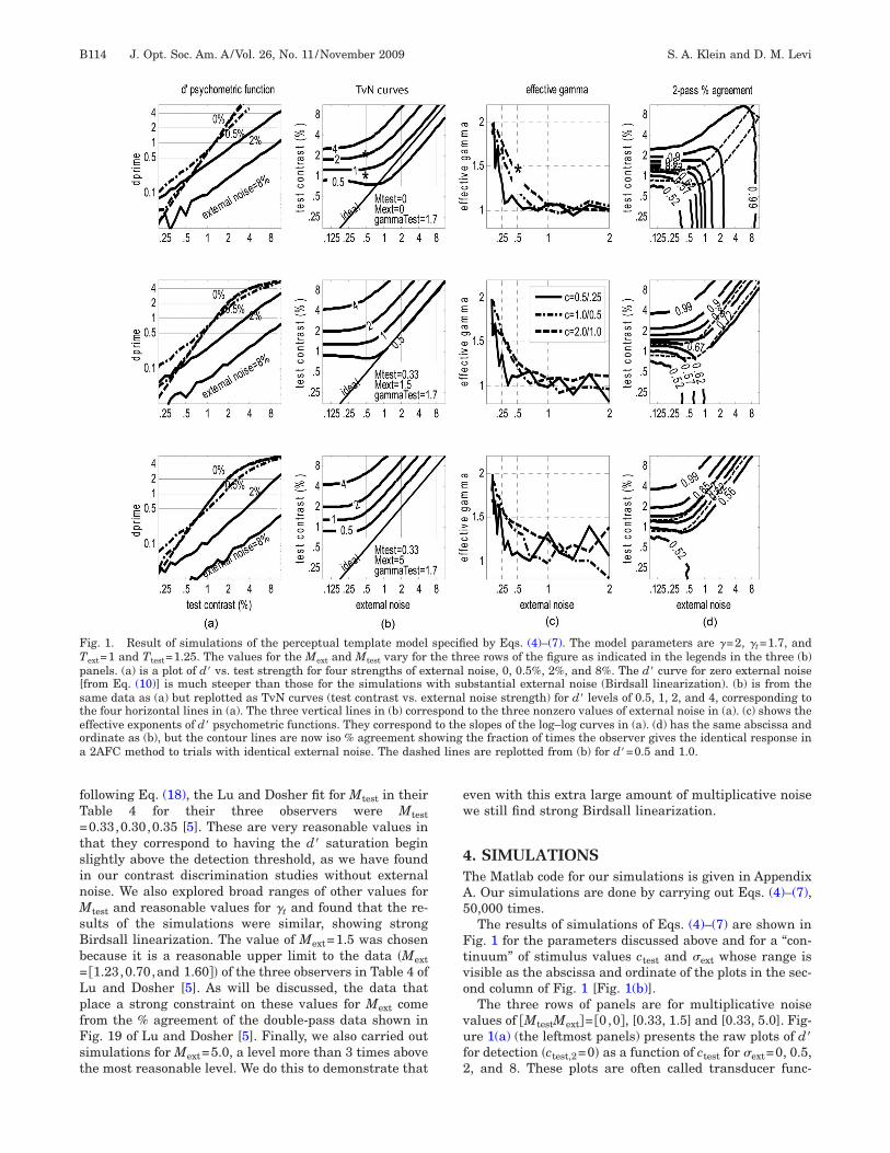

fT=tsinMsBb=LpfFst

ew

4TA5

Ftvo

vuf2

FTp[steoa


ollowing Eq. (18), the Lu and Dosher fit for Mtest in theirable 4 for their three observers were Mtest0.33,0.30,0.35 [5]. These are very reasonable values in

hat they correspond to having the d� saturation beginlightly above the detection threshold, as we have foundn our contrast discrimination studies without externaloise. We also explored broad ranges of other values fortest and reasonable values for �t and found that the re-

ults of the simulations were similar, showing strongirdsall linearization. The value of Mext=1.5 was chosenecause it is a reasonable upper limit to the data �Mext�1.23,0.70,and 1.60�� of the three observers in Table 4 ofu and Dosher [5]. As will be discussed, the data thatlace a strong constraint on these values for Mext comerom the % agreement of the double-pass data shown inig. 19 of Lu and Dosher [5]. Finally, we also carried outimulations for Mext=5.0, a level more than 3 times abovehe most reasonable level. We do this to demonstrate that

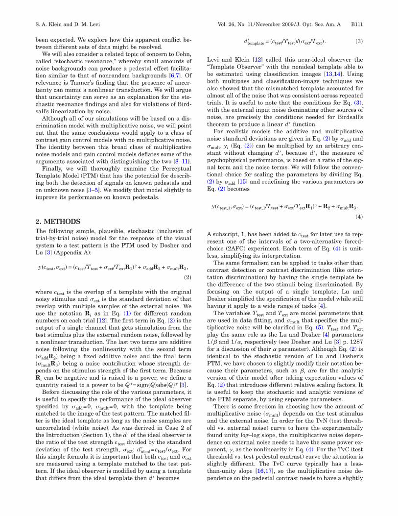
ig. 1. Result of simulations of the perceptual template modelext=1 and Ttest=1.25. The values for the Mext and Mtest vary foranels. (a) is a plot of d� vs. test strength for four strengths of exfrom Eq. (10)] is much steeper than those for the simulations wame data as (a) but replotted as TvN curves (test contrast vs. exhe four horizontal lines in (a). The three vertical lines in (b) correffective exponents of d� psychometric functions. They correspondrdinate as (b), but the contour lines are now iso % agreement sh2AFC method to trials with identical external noise. The dash

ven with this extra large amount of multiplicative noisee still find strong Birdsall linearization.

. SIMULATIONShe Matlab code for our simulations is given in Appendix. Our simulations are done by carrying out Eqs. (4)–(7),0,000 times.The results of simulations of Eqs. (4)–(7) are shown in

ig. 1 for the parameters discussed above and for a “con-inuum” of stimulus values ctest and �ext whose range isisible as the abscissa and ordinate of the plots in the sec-nd column of Fig. 1 [Fig. 1(b)].

The three rows of panels are for multiplicative noisealues of �MtestMext�= �0,0�, [0.33, 1.5] and [0.33, 5.0]. Fig-re 1(a) (the leftmost panels) presents the raw plots of d�or detection �ctest,2=0� as a function of ctest for �ext=0, 0.5,, and 8. These plots are often called transducer func-

ed by Eqs. (4)–(7). The model parameters are �=2, �t=1.7, andee rows of the figure as indicated in the legends in the three (b)noise, 0, 0.5%, 2%, and 8%. The d� curve for zero external noisebstantial external noise (Birdsall linearization). (b) is from thenoise strength) for d� levels of 0.5, 1, 2, and 4, corresponding toto the three nonzero values of external noise in (a). (c) shows theslopes of the log–log curves in (a). (d) has the same abscissa andthe fraction of times the observer gives the identical response ins are replotted from (b) for d�=0.5 and 1.0.

specifithe thrternalith suternalspondto the

owinged line

tsans

s

wpgs1a[ini1tfca

wlpdcuh

scharsqcOtdpp(btiacb

f�gtoh

1Tnpb

acbpo4titftPiaT=tim

tn(i

Tst

fanuchdba

p�mtipF1nnaEsicc


ions. We prefer to call them d� psychometric functionsince d� is directly related to the 2AFC probability correctnd since complexities associated with multiplicativeoise or stimulus uncertainty or gain control distort theirhape from what goes on at the early transduction stage.

The case �ext=0 in the three panels of Fig. 1(a) arehown as a dashed curve, given by Eq. (10) to be

d� = �ctest/1.25��/�1 + Mtest2�ctest/1.25�2�t�1/2, �11�

here �=2 and �t=1.7 as discussed above. In the upperanel of Fig. 1(a) �Mtest=0�, this dashed curve ��ext=0� isiven by d�= �ctest /1.25�� so on the log–log axes it is atraight line of slope �=2. The lower two panels of Fig.(a) show the dramatic change in slope of the d� functions external noise is added. The third column of panelsFig. 1(c)] give the effective ��eff� of the simulations, andt is seen that �eff is indeed equal to 2 for zero externaloise. In order to show how �eff was calculated, an aster-

sk is placed on one of the points in the upper panel of Fig.(c). The three curves in Fig. 1(c) are for three ranges ofest contrast used for calculating the effective slope. Theormula used for �eff is based on the assumption that lo-ally d��c��kc�eff. Thus d��c� /d��c /2�=c�eff / �c /2��eff=2�eff,nd

�eff�ctest� = log�d��ctest�/d��ctest/2��/log�2�, �12�

here d� is shown in panels 1(a) and 1(b) from the simu-ations. This is the log–log slope of the d� function. Theoint with the asterisk is for �ext=0.5 and ctest=2 [theashed curve in Fig. 1(c)]. Asterisks are also placed on theorresponding points for �ext=0.5 and ctest=1 and 2 in thepper panel of Fig. 1(b) to provide further clarification ofow �eff was calculated.When a slight amount of external noise is introduced,

omething unusual occurs as seen in the dotted–dashedurves for �ext=0.5 of Fig. 1(a). The psychometric functionas become shallower than the �ext=0 plot, pivotinground a point below d�=1. By the time the external noiseeaches �ext=1, the log–log slope has fallen to unity ashown in Fig. 1(c), where �eff reaches its asymptotic leveluite rapidly. This dramatic linearization of the d� psy-hometric function is a consequence of Birdsall’s theorem.ne fascinating consequence of the pivoting is that for

est contrasts below the pivot point, d� actually increasedue to the presence of external noise. This facilitationhenomenon has been called stochastic resonance by thehysics community. As will be clarified in the DiscussionSubsection 6.D), it is quite possible that the facilitationy noise is due to uncertainty reduction rather than byhe nonlinear model of Eq. (4). Uncertainty is the compet-ng explanation for both the linearization of the TvC (dis-ppearance of the dipper at high noise levels) and the fa-ilitation (stochastic resonance at low noise levels) as wille clarified in Subsection 6.D.Figure 1(b) is the same data as Fig. 1(a) but plotted dif-

erently (see Appendix A) and for a continuum of values ofext. Figure 1(b) plots the values of ctest that are needed toive d� values of 0.5, 1, 2, and 4. Note that the values forhe levels were chosen to be equally spaced on log–log co-rdinates. These d� levels are indicated in Fig. 1(a) by theorizontal lines, just as the external noise levels of Fig.

(a) are indicated in Fig. 1(b) by the three vertical lines.he plots in Fig. 1(b) are the commonly used threshold vs.oise, TvN, plots. As seen in the Matlab program of Ap-endix A, the TvN plots of Fig. 1(b) are simply producedy Matlab’s “contour” function.Birdsall’s theorem is “evident” in these Fig. 1(b) plots

s we note that the TvN curves for d�=0.5 and 1 areloser together for �ext�1 than for �ext�1. Quotes haveeen placed around the word (evident) because it isn’terceptually evident. One must use a ruler to convinceneself because of an illusion that the tilted lines at5 deg appear closer together than their vertical separa-ion indicates. Surprisingly, this illusion was also presentn a demonstration of Birdsall linearization in Fig. A1 ofhe appendix of Dosher and Lu [3] that shows resultsrom the stochastic PTM! Again a ruler is needed to seehe stunning Birdsall effect. The analytic version of theTM model is not in accord with these simulations since

t predicts a constant vertical shift of the TvN curves (logxes) for different d� values [see Eq. (19) of Section 6].he Birdsall effect is diminished for the ctest=2.0 to ctest1.0 comparison because for ctest=2 the nonlinear satura-

ion has already begun to linearize the TvC function evenn the absence of external noise. Thus to see the Birdsall

echanism one needs to look at low d� levels.Also shown in Fig. 1(b) is a straight line representing

he ideal observer prediction for �add=�mult=0 (no inter-al noise). As was discussed for Case 2 in the IntroductionSection 1) and in the discussion leading to Eq. (3), thedeal observer’s performance is given by

dideal� = ctest/�ext. �13�

he detection or discrimination threshold for the ideal ob-erver plotted in Fig. 1(b) is given by ctest=�ext sincehreshold is defined to be at d�=1.

Also present in Fig. 1(b) is a small stochastic resonanceacilitation that is produced by the external noise. Themount of the dip is less than what is seen in Fig. 1(a)ear d�=0.1 because the dip appears only for very low val-es of d�. It is gone by d�=1. In Fig. 1(b) the dip is for theurve with d�=0.5, corresponding to the lowest of theorizontal lines in Fig. 1(a). If we had plotted the case of�=0.1, a deeper dip (on log axes) would have been found,ut the percent error of the curves make measurementst such low values of d� impractical.As pointed out following Eq. (10), the data for the d�

sychometric function for the zero external noise case�ext=0� can determine Ttest, Mtest, � and �t. Left undeter-ined in Eqs. (4) and (5) are Text and Mext. Unfortunately

hese two parameters are highly correlated and the datas sufficiently noisy that they are not able to be accuratelyinned down based on the discrimination data shown inigs. 1(a)–1(c), This is because all the TvN curves of Fig(b) can be shifted right or left either by multiplicativeoise or by the unknown sensitivity of the template to theoise, Text. This ambiguity is especially apparent in thenalytic version of the PTM as will be explicitly shown inqs. (22) and (23). Lu and Dosher realized this problem,o they made use of the double-pass method for estimat-ng the amount of multiplicative noise [5]. The ambiguityan also be resolved using classification images, as is dis-ussed in Levi et al. [14]. By combining both classification

idc

Eair(isdcntdbaondts

5FnaoatthpcsSatmsadpn(

aoas2sddsscpt

nslanit16Dez

FntndltTp


mages and the double-pass method one has the ability toetect additional sources of double-pass consistency notaptured by the classification-image template.

The double-pass method repeats trials using the sameqs. (4) and (6) values for ctest,1, ctest,2, �test, R1 and R4nd with the additive and multiplicative noise free to varyn the second pass [21]. One then calculates the percent ofesponses that are in agreement in the repeated trialsthe line agree=mean�w2= =w1�, in the Matlab programn Appendix A). Figure 1(d) is a contour plot with theame axes as Fig. 1(b), but now the contour lines are theouble-pass % agreement. Figure 1(d) shows that theseontour lines are sensitive to the amount of multiplicativeoise. The double-pass data together with the location ofhe TvN curves at large values of noise are able to pinown Text and Mext, the two parameters not determinedy the �ext=0 data discussed above. The plots of Fig. 1(d)re a complement to the more common Burgess-type plotsf % correct vs. % agreement that will be discussed in theext section. The two dashed curves in Fig. 1(d) are the�=0.5 and 1.0 curves from Fig. 1(b). They are presentedo show a region where the double-pass constraint can re-trict parameters effectively.

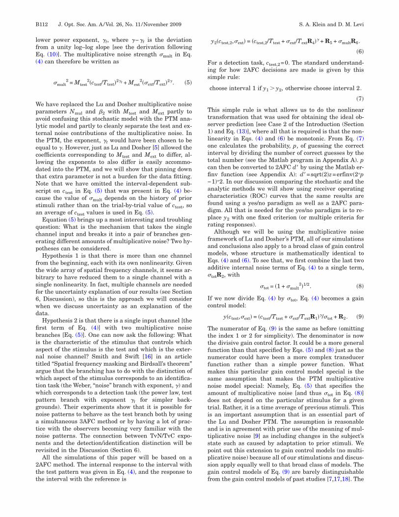
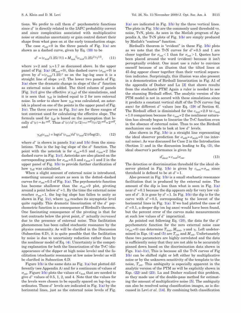
. RESULTS OF EXPERIMENTSigure 2 summarizes our experiments, averaged over fiveormal observers and representing in excess of 40,000 tri-ls on contrast detection of a Gabor, bar-like pattern inne-dimensional noise. Details of the stimuli and methodsre given in Levi et al. [14]. However, here we emphasizehat particular attention was given to minimizing uncer-ainty in the experiments. Specifically, the stimulus was aighly localized bar-like pattern with fixed phase and aosition that was clearly marked by a fixation line adja-ent to the target. Without that fixation line there wouldurely have been position uncertainty of the test pattern.econd, it was presented with a long duration �0.75 s�,nd the onset was clearly marked by a tone, minimizingemporal uncertainty. Third, for each noise level, perfor-ance was measured using the method of constant

timuli (four signal contrasts including a blank) that en-bled us to measure d� at three contrast levels. Finally,ata were collected in runs of 410 trials, preceded by 20ractice trials. Each condition (identical signals andoise) was performed three or four times in separate runs1230–1630 trials), before moving to the next condition.

The format of Fig. 2(a) is the same as that of Fig. 1(a),nd Fig. 2(b) is the same as that of Fig. 1(c). The abscissaf Fig. 2(a) is the peak contrast of the Gabor test patch,nd the ordinate is the d�. The five sets of data, coded byymbol size, are for five noise strengths of 0, 2, 5, 10, and0 NTU (noise threshold units), and 5 NTU means a noisetrength 5 times the noise detection threshold. The noiseetection threshold was measure separately. The noiseetection threshold has special relevance to TvN plotsuch as those shown in Fig. 1(b) because Levi et al. [13,14]howed that the noise detection threshold is typically verylose to the equivalent input noise, Neq, that is the kinkoint in the TvN curves. Equation (23) expresses Neq inerms of Text and Mext.

On log–log axes the d vs. test contrast plot for each
�
oise strength falls remarkably close to being on atraight line (power functions fitted to the data). The log–og slopes of these lines are shown in Fig. 2(b), where thebscissa is in NTU and the ordinate is the effective expo-ent, �eff, of the d� psychometric function. The plot shown

n Fig. 2(b) with a rapid decay to �eff=1, is well matchedo the results of the stochastic PTM model shown in Fig.(c). However, as will be noted in the Discussion (Section), there are also experiments, including that of Lu andosher [5] where the d� exponent in moderate and highxternal noise is barely different from the exponent atero external noise. Uncertainty reduction models will be

ig. 2. Reanalysis of the data of Fig. 15 of Levi et al. [14] for fiveormal observers. (a) is similar to Fig. 1(a), except that the ex-ernal noise is specified in noise threshold units (NTU) (see theumbers above the data). NTU=2 means the noise was twice itsetection threshold at d�=1. The abscissa and ordinate show thatogarithmic axes are being used. (b) is the effective exponent ofhe d� function and is given by the log–log slope of the data in (a).here is a dramatic reduction of the slope once external noise isresent, as would be suggested by Birdsall’s theorem.

cl

tmldr[cta=03tpcFidainwm1tBb�oi(=f

nptnttrtsctmto=

APFfooog

sm

zmscafit

Fpbatlrmsasncags


onsidered as a possible explanation for the apparent vio-ation of Birdsall’s theorem in those experiments.

It is important for our Birdsall theorem argument inhe context of the PTM to place limits on the amount ofultiplicative noise. If it is much larger than the postnon-

inearity external input noise, then the assumptions un-erlying Birdsall’s theorem wouldn’t hold. Data that iselevant to this question come from Fig. 2 of the Levi et al.14] study that shows the square root of detection effi-iency of the data in our Fig. 2. For the normal observershe human to ideal threshold ratio is about 1/0.55=1.82nd the template to ideal threshold ratio is about 1/0.81.25. Thus the human-to-template ratio is about.8/0.55�1.45. As discussed at the beginning of Section, we have fixed the parameters of all of our simulationso have Ttest /Text=1.25, to be in agreement with the tem-late inefficiency that is found in normal observers. Thishoice can be validated by inspection of the top panel ofig. 1(b), where the d�=1 TvN curve is elevated above the

deal observer prediction by a factor of about 1.25. The�=1 TvN curve in the middle panel of Fig. 1(b) is almostfactor of 2 above the ideal observer prediction, compat-

ble with the factor of 1.82 for the Levi et al. (Fig. 2) [14]ormal observers mentioned above. This middle panelith the multiplicative noise parameter of Mext=1.5atches the human data estimate calculated above of

.45 very well. As seen in the middle panel of Fig. 1(c),his amount of multiplicative noise still has a dramaticirdsall theorem decline in the effective exponent. Theottom panels of Fig. 1 are for the case of more than tripleMext=5� the amount of multiplicative noise exhibited byur human observers. Yet the effect of Birdsall’s theorems still present and especially visible at low d�. Our Eq.18) provides further evidence that our value of Mext1.5 is near the upper limit of the experimental values

ound by Lu and Dosher [5].Further validation that the amount of multiplicative

oise must be relatively small is provided by the multi-ass agreement data in Fig. 16 of Levi et al. [14]. Acrosshe entire range of spatial frequencies the ratio of randomoise power to total noise power is between 0.4 and 0.6 forhe normal observers. This is for data with substantial ex-ernal noise, so the internal noise is negligible and theandom noise is entirely multiplicative noise. Thus thehreshold elevation due to the random noise is a factor ofqrt(2) larger than the consistent noise (the sqrt is be-ause Fig 16 is for power rather than contrast). This fac-or is compatible with the factor of 0.8/0.55=1.45. Asentioned above in connection with threshold elevation,

his amount of multiplicative noise matches that found inur simulations for the multiplicative noise being Mext1.5.

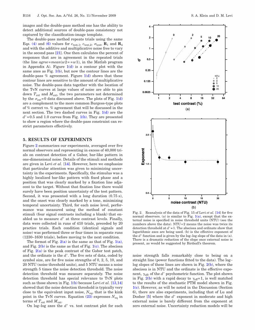
. Double-Pass Data of Lu and Dosher and the Burgesslotsigure 19 of Lu and Dosher [5] presents double-pass data

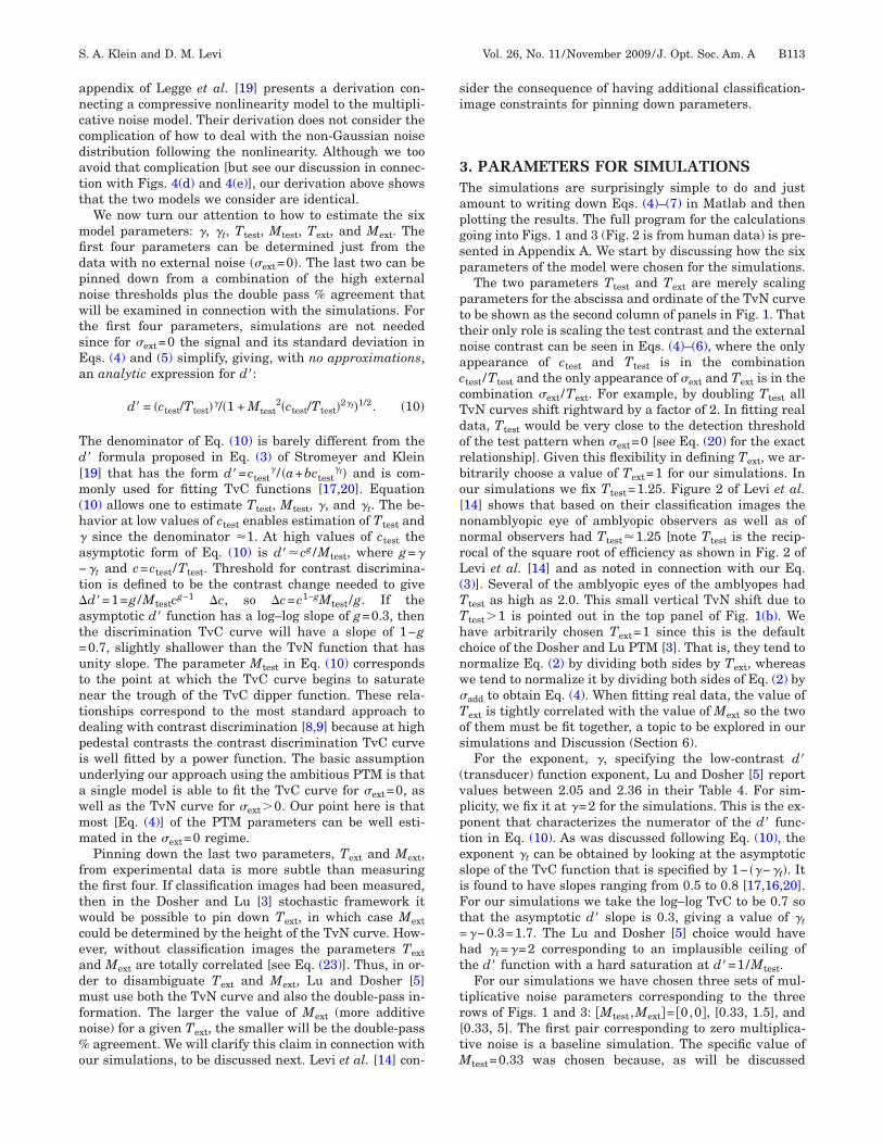
rom their three observers plotted in a Burgess-style plotf % correct vs. % agreement for a 2AFC method [21]. Inrder to make contact with their data, in Fig. 3 we replotur Fig. 1(c) in the more common Burgess format. Beforeetting to the Lu & Dosher data [5] (Fig. 19) we discuss

everal enhancements to the usual Burgess plots that areade in Fig. 3.One enhancement is an analytic formula for the case of

ero external noise ��ext=0�. This is the leftmost (theinimum) part of the allowable values for pagree that is

hown as a thick curve. This case is especially simple be-ause the correlation of responses in the two repeated tri-ls is zero, i.e., if the probability of being correct in therst interval is p, then the probability of being correct inhe second interval is also p. Thus the probability of

ig. 3. The double-pass % agreement data from Fig. 1(c) is re-lotted “inside-out” with axes following the Burgess and Col-orne [21] diagram. The three panels have the same parameterss Fig. 1. The axes are the % agreement and % correct with con-our lines being strength of test pattern and external noise. Theeftmost parabola is independent of model parameters and rep-esents the limiting case where the probability of a correct judg-ent does not depend on the particular external noise being

hown. It is seen that as the external noise increases, the %greement also increases. Also shown are lines of constant signaltrength of ctest=0.5, 1.0, and 2 as well as lines of constant exter-al noise. The positive slope at the left portion of the ctest=0.5urve shows the stochastic resonance effect. The horizontal linet 76% correct �d�=1� shows how the % agreement can distin-uish among the three values of Mext=0, 1.5, and 5.0 that arehown in the three panels.

ar

aoapisc

fnpata1zttentt

%atoittra

BTtahmtgs

Aspn[ccitn

tastae

ucitcccaeusm

mtnsfitccwte

6AOdttrtasoon

[ctdfsMFfHttfitt


greement is the probability of both intervals being cor-ect plus both being incorrect:

pagree-min = p2 + �1 − p�2 = 12 + 2�p − 1

2�2 for �ext = 0,

�14�

nd it is seen that the Burgess curve is a simple parabolaf pagreement as a function of the probability correct, p. Thisnalytic curve for pagree-min is independent of any modelarameters. This curve of minimum agreement is the lim-ting case as the multiplicative noise increases, as can beeen in the three panels where the multiplicative noise in-reases from Mext=0 to 5.

A second innovation in our plots is that we present aew iso-test strength curves as well as the iso-externaloise curves on the plot. The resulting “spiderweb” meshrovides all the information linking % correct and %greement to the stimulus parameters that had requiredwo plots [Figs. 1(b) and 1(d)] previously. Finally, we makeconnection with the d�=1 curves that are shown in Figs.(b) and 1(c). In Fig. 3, the d�=1 curve is simply the hori-ontal line at p=76% that corresponds to d�=1 for a 2AFCask. We extend the d�=1 line to the rightmost portion ofhe % agreement, corresponding to higher values of thexternal noise. For increasing amounts of multiplicativeoise the % agreement saturates. For Mext=1.5 and 5.0he saturation is at 76% and 71%, respectively, as seen inhe vertical line that intersects the d�=1 point.

For all three of observers in Lu and Dosher’s Fig. 19 theagreement is at least 70% correct at d�=1 �p=76% �,

nd for observer SJ, pagree is greater than 80% [5]. For SJhis large amount of agreement means Mext�1.5. For thether two subjects Mext�3. Any larger values would haventroduced more randomness that would have degradedhe % agreement. Yet even for values as large as Mext=5,he bottom panel of Fig. 1(d) shows that Birdsall’s theo-em holds. The Discussion (Subsection 6.A) will examinenother aspect of SJ’s interesting results.

. Departures from the PTM in Amblyopic Visionhe preceding discussion was based on the PTM assump-ion that before the nonlinearity only the fixed, system-tic noise coming from the external noise was present. If,owever, the template has trial-to-trial instability [23], asay be expected in the presence of stimulus uncertainty,

hen a random multiplicative term, whose strength isiven by Mearly, would be present before the nonlinearity,o Eq. (4) becomes

y�ctest,1,�ext� = �ctest,1/Ttest + �ext/TextR1 + �extMearlyRm��

+ R2 + �multR3. �15�

fluctuating template is multiplicative because thetronger the external noise, the stronger will be the out-ut of the fluctuating template. Evidence for this earlyonlinearity may be found in several figures of Levi et al.14] data on amblyopes. Their Fig. 6 shows degraded effi-iency in the presence of noise; their Fig. 12 shows de-reased % agreement, yet Fig. 16 shows as much linear-zation as in normal observers. Thus, by departing fromhe PTM model and by putting some of the multiplicativeoise before the nonlinearity, one is able to have arbi-

rarily large amounts of Birdsall linearization even withrbitrarily large amounts of multiplicative noise. Ithould be noted that Mearly isn’t an extra parameter sincehe extra amount of pre-nonlinearity noise could bechieved by a reduction of the previously present param-ter, Text.

If one calls the fluctuating template a case of templatencertainty, then we have the curious situation that un-ertainty can either increase or decrease the d� nonlinear-ty. Template uncertainty, as in Eq. (15), that comes beforehe nonlinearity will have the effect of linearizing the psy-hometric function (reducing the dipper facilitation in aontrast discrimination task). However, decision stage un-ertainty about which mechanism has the signal will acts an accelerating nonlinearity even at large amounts ofxternal noise. This latter, more standard, definition ofncertainty cannot be put into the single-channel formulauch as Eq. (15) because that form of uncertainty requiresultiple channels.In summary, data from human observers show a dra-atic drop in the effective exponent of the d� vs. test con-

rast plot as the external noise increases. This finding isot surprising since the simulations showed that for theseame observers the amount of multiplicative noise is suf-ciently low �Mext�3� that for the stochastic PTM the ex-ernal noise provides strong linearization of the d� psy-hometric function. That is, the dipper is removed. Onehallenge that needs to be addressed in the Discussion ishy are there such a diversity of data with no lineariza-

ion [4,5,22], modest linearization [15,24], or strong lin-arization [14,25]?

. DISCUSSION. Experimental Conditions and Uncertaintyur data in Fig. 2 show that once external noise is intro-uced, the effective exponent of the d� psychometric func-ion falls dramatically from a value above 2 for zero noiseo a value very close to 1, consistent with Birdsall’s theo-em. However, there is a great mixture of findings on thisopic. This is quite perplexing. Why should there be suchdiversity of findings? This section will consider the pos-

ibility that the diversity of results is due to the diversityf uncertainty across experimental conditions and acrossbservers [26]. But we first examine a representativeumber of these discordant findings.The psychometric functions found by Lu and Dosher

4,5] and Dosher and Lu [3] consistently show strongly ac-elerating functions with similar slopes independent ofhe amount of noise masking including the no-noise con-ition. Pelli [22] shows a similar strong dipper functionor both with noise and no noise, with the dipper being theign of a steeply accelerating psychometric function.any reports, on the other hand, show a mixed finding.igure 1(a) of Goris et al. [15] shows that the no-noise d�

unction is much steeper than when noise is present.owever, full linearization is not achieved, as is seen by

he presence of the dipper in their Fig. 1(c), indicatinghere is still more acceleration of the d� function than wend in our Fig. 2 or than in our Birdsall theorem predic-ions in Fig. 1. Henning and Wichmann [24] have a mix-ure of results across subjects, with observer GBH show-

idtcbn“fteliasmtHsc

wiewpalnaii1bd�0tob

KdodatjlTia

edmwtfHrii

trwptwwsddat[mppmnif[etsdctGtveofifidcni

h“mpeftternstp

tsisnptt


ng a very deep dipper in the no-noise condition. Theipper pretty much disappears in the white-noise condi-ion. On the other hand, observer NAL shows a relativelyonstant dipper across conditions, while TCC’s dipper isetween the other two. It is worth pointing out that Hen-ing and Wichmann [24] also had a condition withnotched noise” where the noise background had a noise-ree notch, nearly two octaves in width, with the test pat-ern in the center. This notched noise was the most pow-rful of all maskers in raising thresholds and also ininearizing the psychometric function. One would hesitaten calling this linearization a Birdsall linearization sincen observer with a well-matched template would barelyee the noise at all. Their finding provides a wonderful re-inder that there is still much to learn about the detec-

ion of targets in noise. Happily, Goris, Wichmann, andenning [27] have more recently developed a quite plau-

ible model based on detailed physiological reasoning thatan account for their surprising data.

Since even a small departure from constancy of slopeill cause a problem for the analytic version of the PTM,

t is useful to look closely at another case of partial lin-arizing in the Lu and Dosher [5] data for observer SJ. To-ard the end of the Results section (Section 5), weointed out that observer SJ had a substantially largermount of % agreement than the other two subjects. Aarger % agreement could be a sign of less multiplicativeoise and/or less uncertainty. Inspection of Fig. 20 of Lund Dosher [5] shows that indeed the high % agreements associated with a reduction of the effective d� exponentn going from �eff�2.5 in the no-noise condition to around.8 in the presence of noise. This exponent was calculatedy comparing the threshold ratios for their top plot for�=1.47 �pcorrect=85% � to their bottom plot for d�=0.54

pcorrect=65% �. Although it may not be significant at the.05 level for a slope change, that datuma is worth men-ioning because it also shows a stochastic resonance hintf facilitation by the noise, a topic soon to be consideredelow.One of the most interesting reports of mixed findings is

ersten’s [25] (Table 2) finding in two observers that theetection of low-spatial-frequency bars (0.25 deg in width)n a blank field had slopes of �=2.34 and 2.86, and with aynamic white-noise background the slopes were �=1.15nd 1.04. However, for thin bars (0.016 deg in width) onhe same dynamic noise, the slopes for the same observersumped to �=2.67 and 2.62! Legge et al. (Table 1) [19] rep-icated the wide bar finding of very strong linearization.hese results on how the stimulus can affect slope linear-

zation are compatible with an uncertainty explanation,s we now consider.We believe that an important contribution to the differ-

nces in Birdsall linearization between datasets may beue to differences in uncertainty associated with experi-ental considerations. In Kersten’s experiments thereould be much more position uncertainty with the very

hin stimuli so any accelerated of the d� function would beound no matter what type of background was present.owever, with the wider stimuli, position uncertainty is

educed and the noise mask could well be sufficient todentify which are the responsive neurons worth attend-ng, thereby removing the remaining uncertainty and

hereby linearizing the psychometric function. For thiseason our stimuli, discussed in connection with Fig. 2,ere designed to maximize the visual system’s ability torecisely attend to the relevant features of the target. Thearget was a local one-dimensional Gabor-like gratingith approximately two cycles. The location of the peakas carefully identified by short bars at the edge of the

timulus (see the inset of Fig. 1 of Levi et al. [14] for moreetails). The long duration and the presence of one-imensional external noise should dramatically reduceny uncertainty about the orientation and timing of theest pattern. Lu and Dosher [5], Pelli [22], and Goris et al.28] used very brief stimuli. They also used stimuli withultiple cycles (7 c /deg in the Goris case), producing

hase uncertainty. For some of the studies an additionalroblem is that all noise and test conditions were inter-ixed. For example in the Goris et al. [15] study, threeoise powers and ten test pedestal levels were intermixed

n a single run. Lu and Dosher typically intermixed dif-erent noise levels (also see Experiment 2 of Goris et al.28]). Randomizing the noise levels may result in observ-rs using different neuronal populations on some trialshan on others (for example when the noise is weak vs.trong). Even without intermixing conditions, the two-imensional white noise that is typically used provides noues to the observer as to which oriented neurons to at-end. As will be discussed later in connection with theoris et al. finding [15,28] of facilitation by noise (stochas-

ic resonance), we believe uncertainty reduction is also aiable explanation of that effect as well as for the pres-nce of a dipper function ��eff�1�. We are by no meansriginal in suggesting uncertainty as an explanation forndings of the dipper across noise conditions. Pelli [22]ts his data in his Fig. 11 with his uncertainty model andemonstrates the ability of uncertainty to produce the fa-ilitation that is at the left of the dipper. Other mecha-isms are needed to produce the threshold elevation that

s at the right of the dipper.There are reports of data that violate the uncertainty

ypothesis. For example, Legge et al. [21] (p. 400) sayOur data pose an additional problem for the uncertaintyodel. The model predicts that the slopes of detection

sychometric functions should be the same in the pres-nce or absence of external noise. As Table 1 shows, weound lower slopes for detection in noise than for detec-ion in the absence of noise.” Their finding a violation ofhe uncertainty model (also found in their supplementalxperiment of their Fig. 7) bothered us for awhile until weealized that their statement is actually a tautology,amely, that there are some experimental conditions andome observers for whom there is minimal uncertainty athe decision stage and these observers will violate theresumption that there is uncertainty.It is appropriate to bring up the topic of uncertainty in

his special issue of JOSAA dedicated to Tanner and Bird-all because of Tanner’s contribution to our understand-ng of uncertainty. The modern history of uncertainty in aignal detection framework began 48 years ago when Tan-er pointed out [30] that the finding of an accelerating d�sychometric function does not necessarily imply an in-rinsic nonlinear transducer function. The same accelera-ion could be caused by stimulus uncertainty at the deci-

sttufb

BImofiPdadv0dj2ifimt8tTsfppTLspPt

dcTtDmtpdeamataettcDn

CLrdtiipritcqeh1tPnsfoaesstsjaco

swmaiSstcllbinni

DTeaa(htittt


ion stage. Cohn followed this up in his Ph.D. research athe University of Michigan (with Tanner as an adviser) inhe early 1970s with a series of papers in JOSA on signalncertainty [29,31]. These papers showed a nonlinear d�

unction that was definitely due to stimulus uncertaintyecause of controls eliminating alternative mechanisms.

. Fitting TvN Datat is easy to get caught up in the minutiae of data andodels, so it is useful to step back and take a broad view

f what actual TvN data look like and what is needed tot the data. Since this paper has focused on the versatileTM model platform, it is useful to look at the type ofata that the PTM model was design to fit. Before the Lund Dosher [5] paper that included double-pass data, theata to be fitted by the PTM were TvN plots of thresholds. external noise for three d� levels ranging from about.5 to 1.5 (2AFC % correct of 65%, 75,% and 85%). A re-uced PTM (rPTM in Table 4 of Lu and Dosher [5]) with

ust four parameters was adequate for fitting the pre-008 PTM data. The parameters of rPTM were the follow-ng: Ttest (or �) for the d�=1 detection threshold and � fortting the log–log slope in the 65%–75% range, and aultiplicative noise parameter was needed for adjusting

he slope due to the beginning of saturation in the 75%–5% range. A final fourth parameter was needed to adjusthe horizontal location of the kink point of the TvN curve.wo additional parameters would have been needed topecify the Birdsall linearization that specifies how the ef-ective � depends on noise contrast: one to specify the ap-roximate noise contrast at which the linearization takeslace and one to specify the extent of the linearization.hese last two parameters haven’t been needed for fittingu and Dosher’s data because the shapes of their mea-ured psychometric functions have been relatively inde-endent of the amount of external noise, so the analyticTM was ideal for their data. It is the stochastic PTMhat has problems for fitting that constant shape data.

For the stochastic PTM to fit data when � is indepen-ent of �ext, rather than introducing a nonlinearity, oneould fit the data with a flexible amount of uncertainty.he most detailed study applying the uncertainty modelo TvN data was the paper by Eckstein, et al. [32]. Lu andosher [4] compared the Eckstein, Ahumada, Watsonodel to the PTM and found them to be similar in fitting

he earlier data. Lu and Dosher [5] in their Table 4 com-are the PTM to seven other models for fitting their newata and find that the PTM outshines all the other mod-ls. The important point to emphasize here is that if thenalytic PTM does a good job of fitting the data, then thateans shape of the psychometric function is constant-for

ll noise levels and any four-parameter model that is ableo shift the location of the TvN curve (2 parameters) anddjust the spacing of the three d� levels (two more param-ters) should do an excellent job of fitting the data. Only ifhe d� function shape depends on noise strength (a viola-ion of the analytic PTM) or if more types of data are in-luded, such as the double-pass data used by Lu andosher [5] would more than four fitting parameters beeeded.

. Birdsall’s Theoremu and Dosher [5] (p. 67) point out that Birdsall’s theoremests on the assumption that sources of noise before theominant nonlinearity are larger than the noise followinghe nonlinearity. That is correct. However, the nonlinear-ty might magnify the effectiveness of the input noise, sot might be difficult to compare relative magnitudes of in-ut and output noise. It was for that reason that we car-ied out simulations for a simple model with a nonlinear-ty sandwiched between two noise sources. The modelhat we simulated was the Lu and Dosher [4] PTM be-ause it has been applied to a wide variety of importantuestions. To our surprise the nonlinearity magnified theffectiveness of the external input noise beyond what wead expected, and in all the simulations presented in Fig.the input noise was able to effectively linearize the sys-

em, a feature not present in the analytic version of theTM. One needs to worry that maybe the multiplicativeoise parameter, Mext wasn’t strong enough. However, wehowed at the end of the Results section (Section 5) thator Mext�1.5 (second row of panels in Fig. 1) the randomutput noise would have raised thresholds by a greatermount than that indicated by the human efficiency. Yetven with Mext=5, the Birdsall linearization still holds. Aimilar analysis was done looking at the double-pass re-ults of Lu and Dosher [5] where limits can be placed onhe % agreement of the responses when the subjects werehown identical 2AFC stimuli. We showed that the sub-ects had a sufficiently large percentage of agreements at

d�=1 level of performance, that the amount of multipli-ative noise could not have been stronger than the levelsf our simulations with Mext=5.

The above discussion is about whether the strong Bird-all linearization in our data (see Fig. 2) is compatibleith the stochastic PTM of Eq. (4). One should keep inind that there is a simple alternative to the PTM that

llows arbitrary amounts of multiplicative noise and yets compatible with Birdsall linearization. In the Resultsection 5 on amblyopic observers, we introduced the pos-ibility of trial-to-trial fluctuations in the shape of theemplate [23]. That type of fluctuation results in multipli-ative noise that comes before the nonlinearity, so Birdsallinearization would be expected. We suspect that thearge amounts of multiplicative noise that we find in am-lyopes [13,14] together with their strong Birdsall linear-zation would require some amount of multiplicativeoise, such as template instability, to come before theonlinearity, effectively reducing the value of Text as seen

n Eq. (15).

. Stochastic Resonance and Uncertaintyhe stochastic resonance literature suggests that nonlin-ar transducer functions will produce facilitation by noiset low d� levels. At Ted Cohn’s memorial service one of theuthors (SK) focused his talk on the stochastic resonanceSR) research Ted had been doing in the last two years ofis life. There is no question that in a system with a hardhreshold the presence of noise can act as a pedestal, lift-ng a very weak signal above threshold. In fact, the leftwo columns of panels of Fig. 1 (Figs 1(a) and 1(b)) showhat the stochastic PTM for low d� levels does show facili-ation by noise. This effect has also been found experi-

mGtticcspcwaSdTbTmt3htobplktwtneaptisttsn

tDbwscweopbcasvctdnn

t[Ctnefh

EBdmtppsnaa2dpwememfstacafsce[sd+mra

FOtmasnI

etpcwo


entally, first by Blackwell [33] and more recently byoris et al. [28,15]. The same question that came up for

he Birdsall effect comes up regarding the mechanism ofhis facilitation by noise. Is it due to the early nonlinear-ty such as found in the stochastic PTM or is it due to un-ertainty, or both? Cohn believed it was an artifact of un-ertainty reduction. He felt that nobody had doneufficiently well-controlled experiments to eliminate theossibility that the accelerated d� function is due to un-ertainty reduction rather than to a transducer functionith ��1. In a posthumously published paper [34] Cohnnd colleagues provide the first convincing evidence thatR in a human sensory system is due to uncertainty re-uction rather than an accelerated transduction process.he experiments involved detection of a rectangular vi-ration pulse applied to a finger with and without noise.he somatosensory system was best for this purpose sinceost of the human SR research has been in the touch sys-

em. A 2AFC method was used with both intervals having00 ms noise bursts and with one of the intervals alsoaving the rectangular pulse. In talks and discussionswo years before his article with Perez, Ted had pointedut that an alternative explanation of the SR data coulde that the presence of the noise acted to reduce the tem-oral uncertainty of when the test stimulus would be de-ivered. He pointed out that a simple control experiment,eeping the noise on continuously, could address this al-ernative hypothesis. An early nonlinearity explanationould still predict facilitation by the noise, but the uncer-

ainty reduction hypothesis predicts that with continuousoise there would be no SR-like facilitation. That controlxperiment was performed in the Perez et al. [34] papernd the data were clearly in favor of the uncertainty ex-lanation rather than the nonlinear transducer explana-ion. Blackwell [33] came to a similar conclusion by show-ng that SR facilitation was present for detection ofinusoids with a noise masker far outside the pass band ofhe test pattern. This is an excellent argument for facili-ation due to reduction of uncertainty in the timing of thetimulus, providing a viable alternative to rectificationonlinearities that enable a PTM type facilitation.This discussion is relevant to our Birdsall effect inves-

igation for two reasons. First, as pointed out by Lu andosher [4,5], the main contender to the PTM model haseen the uncertainty model of Eckstein et al. [32]. Thuse should remain open minded about the possibility that

ome amount of uncertainty reduction needs to be in-luded in explanations of the detection of signals in noisehen the noise strength is low, as it is in both Birdsall lin-arization and in facilitation by noise. Second, the themef the Goris et al. [15] paper is given by the title of theiraper “Modelling contrast discrimination data suggestoth the pedestal effect and stochastic resonance to beaused by the same mechanism.” They find that weakmounts of noise produce both some SR facilitation andome Birdsall linearization. They happen to argue in fa-or of a PTM-like stochastic model or the equivalent gainontrol model. Goris et al. [28] say in their abstract thathat “Both simple uncertainty reduction and an energyiscrimination strategy can be excluded as possible expla-ations for this effect” (referring to the SR facilitation byoise). However, in the first section of the Discussion (Sec-

ion 6) we pointed out a number of aspects of the Goris15,28] methods that would magnify uncertainty. Untilohn’s simple manipulation of leaving the noise on con-

inuously is carried out, we believe the uncertainty expla-ation is equally viable. The variability of the Birdsall lin-arization and the noise facilitation across subjects mayavor the uncertainty explanation. We look forward toaving this uncertainty of explanations resolved.

. Multiplicative Noise vs. Saturating Transducerehind much of the interest in the shape of the trans-ucer function (c� in the present case) and the extent ofultiplicative noise is the desire to connect psychophysics

o underlying mechanisms that could possibly be testedhysiologically. It is thus not surprising that just as thisroblem has been investigated using the task of detectingignals in noise, it has also been investigated using sig-als with the same signal as a pedestal. Recently severalrticles have been published based on the Kontsevich etl. [8] (KCT) contrast discrimination dataset. KCT usedAFC with hundreds of trials at each of more than aozen pedestal levels. They argued that their dataointed to a large amount of multiplicative noise togetherith a constantly accelerating transducer function. Thensuing articles pointed out the difficulty of pinning downultiplicative noise vs. a saturating transducer function,

specially when based on 2AFC data. Part of the argu-ent hinges on the issue that assuming a particular form

or the underlying transducer function (c� both for Kont-evich et al. and for Lu and Dosher) was much too restric-ive. Katkov et al. [11] noted that pinning down themount of multiplicative noise was especially difficult be-ause of an intrinsic nonlinearity in the equations. Theyrgued that the Kontsevich data did not provide evidenceor multiplicative noise. Klein [9] agreed that aingularity-like structure was present but that specialharacteristics of the Kontsevich data provided strongvidence for the presence of multiplicative noise. Klein10] provided further evidence for multiplicative noise byhowing that the Kontsevich data failed a just-noticeable-ifference additivity test whereby d��AC�=d��AB�d��BC� (where A, B, C are contrast levels) if there is noultiplicative noise. We suspect that many of the issues

aised in the context of backgrounds known exactly alsopply to noise backgrounds.

. Analytic vs. Stochastic Modelsur analyses in Fig. 1 were based on the fixed-template,

rial-by-trial prediction of the underlying stochasticodel described in the Dosher and Lu [3] appendix. For

ll their data fitting however, Lu and Dosher [4,5] makeeveral strong assumptions about the expectation value ofon-zero-mean Gaussian noise that is raised to a power.n a footnote to Appendix E, Lu and Dosher [5], p. 80, say

“After nonlinear transduction, the distribution of thexternal noise might deviate from the Gaussian distribu-ion. However, spatial and temporal summation in theerceptual system should reduce this deviation. Whenombined with additive and multiplicative noises, both ofhich are Gaussian distributed, we assume that the sumf the noises is approximately Gaussian. However, we re-

sa

wYflttnsdnp

i�TtU

TsnHDonl

ptfrPg[

TtsccsS

wfFcrwfstFobft

c

w=

we

Lttitdfmo

efEtdoTistcnt

o(o�


trict ourselves to performance levels below 90% so as tovoid the tails of the distribution.”

In our simulations we, too, are combining the signalith large amounts of additive and multiplicative noise.et no matter how we manipulate the model, we haveound that Birdsall’s theorem kicks in at levels much be-ow 90% correct (below d�=2). Lu and Dosher commentedhat spatial and temporal summation in the visual sys-em might convert the first term of Eq. (2) into a Gaussianoise distribution. That would be a miraculous conversionince it could connect the analytic PTM model to the un-erlying mechanistic model of Eq. (2). However, that con-ection would involve a transformation of the underlyingarameters that is not yet available.This section will examine the consequences of assum-

ng that �ctest /Ttest+�ext/TextR1�� has an expectation ofctest /Ttest�� and a standard deviation of k��ext/Text��.hat assumption leads to the analytic version of the PTMhat Dosher and Lu have applied to numerous situations.sing our notation the analytic d� for the PTM becomes

d�2 = �ctest/Ttest�2�/�k��ext/Text�2� + 1 + Mtest2�ctest/Ttest�2�t

+ Mext2��ext/Text�2��. �16�

he parameter k appears in the denominator because thetandard deviation of the Gaussian noise followed by aonlinearity term introduces a factor that depends on �.owever, for simplicity of notation we follow Lu andosher [4] in assuming that k=1. The surprise at the end

f this section is that no renormalization of parameters iseeded in going from the stochastic to the analytic formu-

ae if d�=1.We would now like to invert Eq. (16) from being an ex-

ression of d� in terms of ctest to an expression of ctest inerms of d�. It is not possible to get a simple expressionor ctest for arbitrary values of �t. For that reason we willevert to the original PTM and set �t=�. The analyticTM prediction for the threshold signal strength at aiven d� criterion can then be written as [Lu and Dosher5] Eq. (14) transformed to our notation]

�ctest/Ttest�2� = �1 + �1 + Mext2��ext/Text�2��/�1/d�2 − Mtest

2�.

�17�

he only difference from the Lu–Dosher equation (otherhan the minor change in variables) is that we have ab-orbed a factor of 1

2 into our definition of Mtest2 as dis-

ussed earlier. By comparing Eqs. (16) and (17) with theomparable Eqs. (E6) and (E7) of Lu and Dosher [5], weee that their best-fitting parameters for observers CC,J, and WC in terms of our parameters are as follows:

CC SJ WC

� = �t 2.05 2.27 2.36 =�,

Ttest= 0.055 0.048 0.086 =�add1/�/�,

Text= 0.103 0.086 0.128 =�add1/�,

Mext= 1.23 0.70 1.60 =Nmul,

Mtest= 0.33 0.30 0.35 =Nmul��2/��/sqrt�2�,

�18�

here �, �add, Nmul, �, and �2 are the PTM parametersrom Table 4 of Lu and Dosher [5]. In the simulations ofig. 1 the only parameter that can distinguish the sto-hastic and analytic PTM are �, Mext and Mtest. The pa-ameters Ttest and Text are always used in conjunctionith ctest and �ext and thus simply shift the log–log TvN

unctions vertically or horizontally without changinghape or relative position in going from the stochastic tohe analytic PTM. In the simulations of the middle row ofig. 1 we have used parameters closely matched to thosef the Lu and Dosher data [5] presented in Eq. (18). In theottom row of Fig. 1 we increased Mext more than three-old to show that Birdsall linearization holds even athose extreme levels.

On pp. 15–16 of Levi et al. [14] we showed that Eq. (17)an be rewritten as

ctest = Th0C�d��F��ext� �19�

here Th0 is the threshold for �ext=0 at d�=1 since C�1�1 and F�0�=1. Comparing Eqs. (17) and (19) we find

Th0 = Ttest/�1 − Mtest2�1/2� = 0.061, 0.053, 0.096

for the three observers of Eq . �18�. �20�

C�d�� = ��1 − Mtest2�/�1/d�2 − Mtest

2��1/2�. �21�

F��ext� = ��1 + ��ext/Neq�2��1/2�, �22�

here Neq, similar to the equivalent input noise of a lin-ar amplifier model, is given by

Neq = Text/�1 + Mext2�1/2� = 0.083, 0.079, 0.097

for the three observers of Eq . �18�. �23�

evi et al. [13,14] showed that Neq is typically very closeo the noise detection threshold. The values of Neq for thehree observers are quite similar to each other. C�d��, thenverse contrast response function, is proportional to theest contrast as a function of d�, normalized to unity for�=1. Levi et al. [14] not only provide further clarification

or this simpler way of expressing the analytic PTModel, but also suggested modifications to Eq. (16) based

n their data.It is worthwhile examining the meaning of the param-

ters that we have been using, whose best-fitting valuesor the three Lu and Dosher [5] observers are shown inq. (18). Ttest is very close to the contrast threshold for

he Lu and Dosher orientation task. The true threshold at�=1 includes a minor correction term in the denominatorf Eq. (20). The horizontal location of the kink point of thevN curve, obtained by extrapolating its two asymptotes,

s given by a simple combination of Text and Mext ashown in Eq. (23). Finally, the two multiplicative noiseerms, Mtest and Mext, are simply the amount of multipli-ative noise when both the test strength and the externaloise strength have been normalized to unitless quanti-ies by Ttest and Text.

An important outcome of rewriting Eq. (17) in the formf Eq. (19) is that it emphasizes the separability of Eq.17) into the C�d�� term that depends on d� independentf �ext times the last term of Eq. (19) that depends just on

, independent of d . This separability means that the
ext �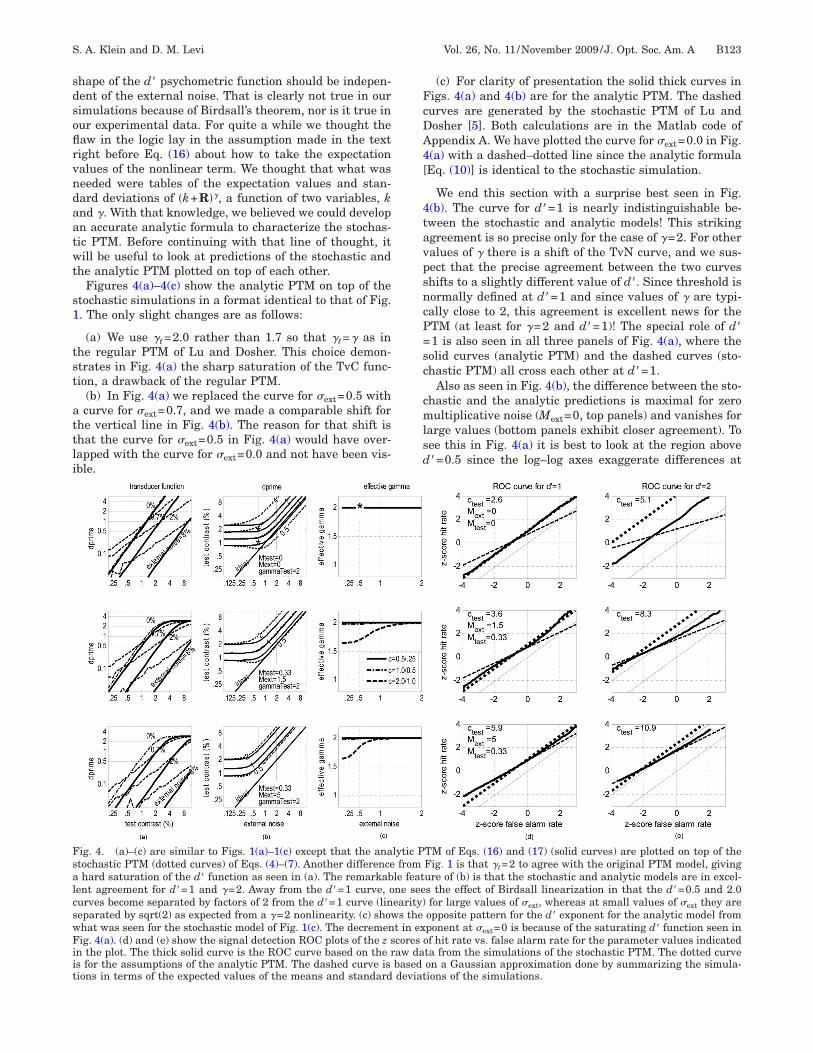

sdsoflrvndaatwt

s1

tst

attli

FcDA4[

4tavpsncP=sc

cmlsd

FsalcswFiit


hape of the d� psychometric function should be indepen-ent of the external noise. That is clearly not true in ourimulations because of Birdsall’s theorem, nor is it true inur experimental data. For quite a while we thought theaw in the logic lay in the assumption made in the textight before Eq. (16) about how to take the expectationalues of the nonlinear term. We thought that what waseeded were tables of the expectation values and stan-ard deviations of �k+R��, a function of two variables, knd �. With that knowledge, we believed we could developn accurate analytic formula to characterize the stochas-ic PTM. Before continuing with that line of thought, itill be useful to look at predictions of the stochastic and

he analytic PTM plotted on top of each other.Figures 4(a)–4(c) show the analytic PTM on top of the

tochastic simulations in a format identical to that of Fig.. The only slight changes are as follows:

(a) We use �t=2.0 rather than 1.7 so that �t=� as inhe regular PTM of Lu and Dosher. This choice demon-trates in Fig. 4(a) the sharp saturation of the TvC func-ion, a drawback of the regular PTM.

(b) In Fig. 4(a) we replaced the curve for �ext=0.5 withcurve for �ext=0.7, and we made a comparable shift for

he vertical line in Fig. 4(b). The reason for that shift ishat the curve for �ext=0.5 in Fig. 4(a) would have over-apped with the curve for �ext=0.0 and not have been vis-ble.

(c) For clarity of presentation the solid thick curves inigs. 4(a) and 4(b) are for the analytic PTM. The dashedurves are generated by the stochastic PTM of Lu andosher [5]. Both calculations are in the Matlab code ofppendix A. We have plotted the curve for �ext=0.0 in Fig.(a) with a dashed–dotted line since the analytic formulaEq. (10)] is identical to the stochastic simulation.

We end this section with a surprise best seen in Fig.(b). The curve for d�=1 is nearly indistinguishable be-ween the stochastic and analytic models! This strikinggreement is so precise only for the case of �=2. For otheralues of � there is a shift of the TvN curve, and we sus-ect that the precise agreement between the two curveshifts to a slightly different value of d�. Since threshold isormally defined at d�=1 and since values of � are typi-ally close to 2, this agreement is excellent news for theTM (at least for �=2 and d�=1)! The special role of d�1 is also seen in all three panels of Fig. 4(a), where theolid curves (analytic PTM) and the dashed curves (sto-hastic PTM) all cross each other at d�=1.

Also as seen in Fig. 4(b), the difference between the sto-hastic and the analytic predictions is maximal for zeroultiplicative noise (Mext=0, top panels) and vanishes for

arge values (bottom panels exhibit closer agreement). Toee this in Fig. 4(a) it is best to look at the region above�=0.5 since the log–log axes exaggerate differences at

ig. 4. (a)–(c) are similar to Figs. 1(a)–1(c) except that the analytic PTM of Eqs. (16) and (17) (solid curves) are plotted on top of thetochastic PTM (dotted curves) of Eqs. (4)–(7). Another difference from Fig. 1 is that �t=2 to agree with the original PTM model, givinghard saturation of the d� function as seen in (a). The remarkable feature of (b) is that the stochastic and analytic models are in excel-

ent agreement for d�=1 and �=2. Away from the d�=1 curve, one sees the effect of Birdsall linearization in that the d�=0.5 and 2.0urves become separated by factors of 2 from the d�=1 curve (linearity) for large values of �ext, whereas at small values of �ext they areeparated by sqrt(2) as expected from a �=2 nonlinearity. (c) shows the opposite pattern for the d� exponent for the analytic model fromhat was seen for the stochastic model of Fig. 1(c). The decrement in exponent at �ext=0 is because of the saturating d� function seen inig. 4(a). (d) and (e) show the signal detection ROC plots of the z scores of hit rate vs. false alarm rate for the parameter values indicated

n the plot. The thick solid curve is the ROC curve based on the raw data from the simulations of the stochastic PTM. The dotted curves for the assumptions of the analytic PTM. The dashed curve is based on a Gaussian approximation done by summarizing the simula-ions in terms of the expected values of the means and standard deviations of the simulations.

ltas

anb�=ltbvptelifspaippc

i(ttv4

cab

Pbdawts�lpctri

stdpmpc

dGvaalaf

tsFttp[icctpGpn

leTwtcmcftct[tnctaft

7WdtunaeuoWafiso


ow d�. Figure 4(b) also shows that for small values of �exthe analytic and the stochastic predictions are the same,s expected from Eq. (10). For larger values of �ext, Bird-all linearization and noise facilitation appear.

The agreement of the analytic and the stochastic PTMt d�=1 can be readily understood for zero multiplicativeoise �Mext=Mtest=0� as follows: For low values of �extoth versions must agree with Eq. (10). At large values ofext the analytic equation [Eq. (17)] gives ctest /Ttestd�1/��ext/Text, while the stochastic PTM after Birdsall

inearization gives ctest /Ttest=d��ext/Text [Eq. (3)]. Thushey agree for d�=1. Only near the kink point will theree a slight, nearly invisible, difference between the twoersions. However, for nonzero values of Mext or Mtest theroblem is more challenging since we are no longer ableo make a simple transformation to eliminate the nonlin-arity. Figures 4(d) and 4(e) present ROC curves that il-ustrate why the stochastic and analytic formulations aren conflict. An ROC curve is a plot of the z scores of hit vs.alse alarm rates. The three rows of panels are for theame conditions as in Figs. 4(a)–4(c) but just for twooints of those plots given by �ext=2 with d�=1 [Fig. 4(d)]nd d�=2 [Fig. 4(e)]. The value of ctest is given by its valuen Figs. 4(a) and 4(b) from the stochastic prediction (therediction with no approximations). The three curveslotted in each panel correspond to three methods for cal-ulating the ROC curves:

Method 1: Stochastic PTM (solid curves). This methods based on histograms of the 50,000 simulation pointssee Appendix A) producing probability distribution func-ions for the blank (false alarms) and the signal (hits) in-ervals. The ROC curve is a plot of the cumulative hit rates. false alarm rate [z scores plotted in Figs. 4(d) and(e)].Method 2: Analytic PTM (dotted curves). The ROC

urve is given by zhit=zfa+danalytic� where fa means falselarm, and d� is given by Eq. (16) (with k=1 as specifiedy the analytic PTM).Method 3: Gaussian approximation to the stochastic

TM (dashed cures). One can improve the analytic PTMy taking expectation values of the mean and standardeviation of the nonlinear term of Eq. (4) and generatingn ROC curve given by: zhit=zfa�fa/�hit+ ��hit−�hit��hit,here �hit and �hit are the mean and the standard devia-

ion of the first term of Eq. (4) and �fa and �fa are theame but with ctest=0. The cross terms of Eq. (4) makehit��fa for ��1 so the ROC slope of the dashed line is

ess than 1, even without multiplicative noise. The multi-licative noise terms of Eq. (4) does not alter the ROCurve because we are following the PTM assumption thathe multiplicative noise is based on an average stimulusather than the particular stimulus in the first or secondnterval.

These ROC curves are generated for a yes–no task of aignal vs. a blank. The 2AFC predictions of d� for rela-ively straight ROC curve (as ours are) is sqrt(2) times theistance from the origin to the ROC curve [35]. The threelots shown in Fig. 4(d) show that for d�=1 the threeethods are in quite close agreement. However, the three

lots of Fig. 4(e) for d�=2, show that the analytic PTMan depart substantially from the correct (stochastic) pre-

iction, as was expected from the previous figures. Theaussian approximation method also has substantial de-iations from the stochastic value. We have not yet beenble to find an analytic expression that provides a goodpproximation to the stochastic model that works both forarge external noise where Birdsall linearization occursnd near the kink point where stochastic resonance isound.

By plotting the analytic and the stochastic predictionsogether as in Fig. 4(b), one obtains a new insight into thetochastic resonance mechanism. In the bottom curves ofig. 4(b), for d�=0.5, facilitation by noise extends beyond

he low-noise-contrast regime. Everyone who has foundhis stochastic resonance facilitation experimentally re-orts that it is found only at very low noise levels15,28,29,36]. However, that is because they are compar-ng thresholds relative to zero-noise performance. If weompare the “true” behavior of the simulation (dottedurves) with the analytic prediction (solid curves) we seehat the facilitation begins slightly below the TvN kinkoint and persists to high external noise. The non-aussian nature of the nonlinearity keeps the facilitationersisting in comparison with the outcome for Gaussianoise.In this paper we did the easy forward model with simu-

ations where we are given a model with known param-ters, and we made predictions of d� and % agreement.he greater challenge lies with the inverse problemhere one is given the data of d� and % agreement and

he goal is to determine the best-fitting model. This is ahallenge because there is no way to rapidly calculate theodel prediction [unless �=2 and d�=1 as discussed in

onnection with Figs. 4(a) and 4(b)]. The standard searchor optimal parameters requires many thousands of itera-ions, so a very rapid model calculation is needed. Onean always invent analytic models, but the more ambi-ious project would be to follow the lead of Lu and Dosher4] to develop a stochastic model that includes the trial-o-trial dependence on the specific sample of externaloise. That model would include improved predictions oflassification images and allow for a noisy template beforehe nonlinearity. A new approach is needed to get a goodnalytic approximation that includes the nonlinear trans-orms of random data. The improved analytic approxima-ion would enable efficient data fitting.

. CONCLUSION AND SUMMARYe began by citing the revolution in our understanding of

etection and identification that took place 50 years agohrough the work of Tanner, Birdsall, and colleagues whoshered in our modern understanding of detection of sig-als in noise. It is interesting that the two compilations ofrticles of direct relevance to their pioneering work weredited by Ted Cohn. The first was the Visual Detection vol-me [1] that Ted edited, published by the Optical Societyf America in 1993. The second, in collaboration withalter Makous was the compilation of articles 24 years

go in a special issue of JOSAA on Detection and Identi-cation [37]. There were many articles in that special is-ue of relevance to the present special issue. We will pointut a few of them. We already mentioned Smith and

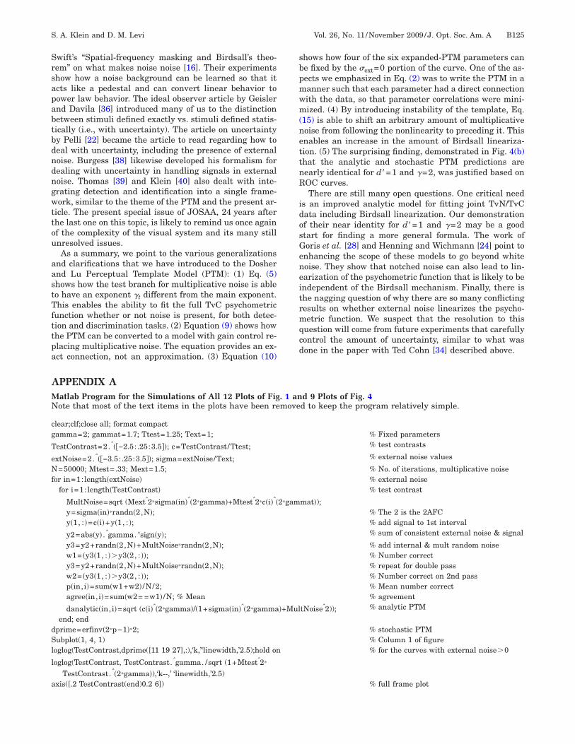
Srsapabtbdndngwttou

aastTfttpa

sbpmwm(nettnR

idosGeneitrmqcd

AMN

cg

T

eNf

dSl

l

a


wift’s “Spatial-frequency masking and Birdsall’s theo-em” on what makes noise noise [16]. Their experimentshow how a noise background can be learned so that itcts like a pedestal and can convert linear behavior toower law behavior. The ideal observer article by Geislernd Davila [36] introduced many of us to the distinctionetween stimuli defined exactly vs. stimuli defined statis-ically (i.e., with uncertainty). The article on uncertaintyy Pelli [22] became the article to read regarding how toeal with uncertainty, including the presence of externaloise. Burgess [38] likewise developed his formalism forealing with uncertainty in handling signals in externaloise. Thomas [39] and Klein [40] also dealt with inte-rating detection and identification into a single frame-ork, similar to the theme of the PTM and the present ar-

icle. The present special issue of JOSAA, 24 years afterhe last one on this topic, is likely to remind us once againf the complexity of the visual system and its many stillnresolved issues.As a summary, we point to the various generalizations

nd clarifications that we have introduced to the Doshernd Lu Perceptual Template Model (PTM): (1) Eq. (5)hows how the test branch for multiplicative noise is ableo have an exponent �t different from the main exponent.his enables the ability to fit the full TvC psychometric

unction whether or not noise is present, for both detec-ion and discrimination tasks. (2) Equation (9) shows howhe PTM can be converted to a model with gain control re-lacing multiplicative noise. The equation provides an ex-ct connection, not an approximation. (3) Equation (10)

hows how four of the six expanded-PTM parameters cane fixed by the �ext=0 portion of the curve. One of the as-ects we emphasized in Eq. (2) was to write the PTM in aanner such that each parameter had a direct connectionith the data, so that parameter correlations were mini-ized. (4) By introducing instability of the template, Eq.

15) is able to shift an arbitrary amount of multiplicativeoise from following the nonlinearity to preceding it. Thisnables an increase in the amount of Birdsall lineariza-ion. (5) The surprising finding, demonstrated in Fig. 4(b)hat the analytic and stochastic PTM predictions areearly identical for d�=1 and �=2, was justified based onOC curves.There are still many open questions. One critical need

s an improved analytic model for fitting joint TvN/TvCata including Birdsall linearization. Our demonstrationf their near identity for d�=1 and �=2 may be a goodtart for finding a more general formula. The work oforis et al. [28] and Henning and Wichmann [24] point tonhancing the scope of these models to go beyond whiteoise. They show that notched noise can also lead to lin-arization of the psychometric function that is likely to bendependent of the Birdsall mechanism. Finally, there ishe nagging question of why there are so many conflictingesults on whether external noise linearizes the psycho-etric function. We suspect that the resolution to this

uestion will come from future experiments that carefullyontrol the amount of uncertainty, similar to what wasone in the paper with Ted Cohn [34] described above.

PPENDIX Aatlab Program for the Simulations of All 12 Plots of Fig. 1 and 9 Plots of Fig. 4ote that most of the text items in the plots have been removed to keep the program relatively simple.

lear;clf;close all; format compactamma=2; gammat=1.7; Ttest=1.25; Text=1; % Fixed parameters

estContrast=2.ˆ��−2.5: .25:3.5��; c=TestContrast/Ttest; % test contrasts

xtNoise=2.ˆ��−3.5: .25:3.5��; sigma=extNoise/Text; % external noise values

=50000; Mtest=.33; Mext=1.5; % No. of iterations, multiplicative noiseor in=1:length�extNoise� % external noise

for i=1: length�TestContrast� % test contrast

MultNoise=sqrt (Mextˆ2*sigma�in�ˆ�2*gamma�+Mtestˆ2*c�i�ˆ�2*gammat�);y=sigma�in�*randn�2,N�; % The 2 is the 2AFCy�1, : �=c�i�+y�1, : �; % add signal to 1st interval

y2=abs�y� .ˆgamma. *sign�y�; % sum of consistent external noise & signal

y3=y2+randn�2,N�+MultNoise*randn�2,N�; % add internal & mult random noisew1= �y3�1, : ��y3�2, : ��; % Number correcty3=y2+randn�2,N�+MultNoise*randn�2,N�; % repeat for double passw2= �y3�1, : ��y3�2, : ��; % Number correct on 2nd passp�in, i�=sum�w1+w2� /N/2; % Mean number correctagree�in, i�=sum�w2= =w1� /N; % Mean % agreement

danalytic�in, i�=sqrt (c�i�ˆ�2*gamma�/(1+sigma�in�ˆ�2*gamma�+MultNoiseˆ2)); % analytic PTM

end; endprime=erfinv�2*p−1�*2; % stochastic PTMubplot(1, 4, 1) % Column 1 of figure

oglog(TestContrast,dprime([11 19 27],:),‘k,’‘linewidth,’2.5);hold on % for the curves with external noise�0

oglog(TestContrast, TestContrast.ˆgamma. /sqrt (1+Mtestˆ2*

TestContrast.ˆ�2*gamma�),‘k--,’ ‘linewidth,’2.5)xis([.2 TestContrast(end)0.2 6]) % full frame plot

ssssep

ASt(mvtm

R

1

1

1

1

1

1

1

1


ubplot(1,4,2); �c ,h�=contour (dprime,’[.5 2 2 4],‘k,’‘linewidth,’2.5);hold on;clabel(c,h) % Column 2ubplot(1,4,2); �c ,h�=contour (danalytic,’[.5 1 2 4],‘r,’‘linewidth,’1.5);clabel(c,h) % Column 2ubplot(1,4,4); �c ,h�=contour (agree,’[.52 .62 .72 .8 .9 .99],‘k,’ ‘linewidth,’2.5); clabel(c,h) % column 4ubplot(1,4,3); effectiveGamma=log (dprime(1:19,[7 11 15])./dprime(1:19,[3 7 11]))/log(2);e=extNoise�1:19�; % Column 3lot(ee,effectiveGamma(:,1),‘k,’ee,effectiveGamma(:,2),‘k-,’ee,

effectiveGamma(:,3),‘--k,’‘linewidth,’2.5);

1

1

2

2

2

2

2

2

2

2

2

2

3

3

3

3

3

3

3

3

3

3

4

CKNOWLEDGMENTSupported by grants R01EY01728 and R01EY04776 fromhe National Eye Institute, National Institutes of HealthNIH). We thank the reviewers for their helpful com-ents. Many discussions with Zhong-Lin Lu have been

ery helpful in clarifying a number of issues covered inhis paper. We also thank Ted Cohn for educating us onany of these interesting topics.

EFERENCES1. T. E. Cohn, ed., Visual Detection, Vol. 3 of Collected Works

in Optics (Optical Society of America, 1993).2. D. J. Lasley and T. E. Cohn, “Why luminance

discrimination may be better than detection,” Vision Res.21, 273–278 (1981).

3. B. A. Dosher and L. L. Lu, “Mechanisms of perceptualattention in precuing of location,” Vision Res. 40,1269–1292 (2000).

4. Z. L. Lu and B. A. Dosher, “Characterizing humanperceptual inefficiencies with equivalent internal noise,” J.Opt. Soc. Am. A 16, 764–778 (1999).

5. Z. L. Lu and B. A. Dosher, “Characterizing observers usingexternal noise and observer models: assessing internalrepresentations with external noise,” Psychol. Rev. 115,44–82 (2008).

6. J. Nachmias and R. V. Sansbury, “Grating contrast:Discrimination may be better than detection,” Vision Res.14, 1039–1042 (1974).

7. C. F. Stromeyer and S. A. Klein, “Spatial frequencychannels in human vision as asymmetric (edge)mechanisms,” Vision Res. 14, 1409–1420 (1974).

8. L. L. Kontsevich, C. C. Chen, and C. W. Tyler, “Separatingthe effects of response nonlinearity and internal noisepsychophysically,” Vision Res. 42, 1771–1784 (2002).

9. S. A. Klein, “Separating transducer nonlinearities andmultiplicative noise in contrast discrimination,” Vision Res.46, 4279–4293 (2006).

0. S. A. Klein, “A local measure for modeling contrastdiscrimination, Response to Katkov, Tsodyks and Sagi,”Vision Res. 47, 2912–2917 (2007).

1. M. Katkov, M. Tsodyks, and D. Sagi, “Singularities in theinverse modeling of 2AFC contrast discrimination data,”Vision Res. 46, 259–266 (2006).

2. D. M. Levi and S. A. Klein, “Classification images fordetection and position discrimination in the fovea andparafovea,” J. Vision 2, 46–65 (2002).

3. D. M. Levi, S. A. Klein, and I. Chen, “The response of theamblyopic visual system to noise,” Vision Res. 47,2531–2542 (2007).

4. D. M. Levi, S. A. Klein, and I. Chen, “What limitsperformance in the amblyopic visual system: seeing signalsin noise with an amblyopic brain,” J. Vision 8, 1.1–23(2008).

5. R. L. Goris, J. Wagemans, and F. A. Wichmann, “Modellingcontrast discrimination data suggest both the pedestaleffect and stochastic resonance to be caused by the samemechanism,” J. Vision 8, article 17, 1–21 (2008).

6. R. A. Smith and D. J. Swift, “Spatial-frequency maskingand Birdsall’s theorem,” J. Opt. Soc. Am. A 2, 1593–1599(1985).

7. G. E. Legge and J. M. Foley, “Contrast masking in humanvision,” J. Opt. Soc. Am. 70, 1458–1471 (1980).

8. J. M. Foley, “Human luminance pattern-visionmechanisms: masking experiments require a new model,”J. Opt. Soc. Am. A 11, 1710–1719 (1994).

9. G. E. Legge, D. Kersten, and A. E. Burgess, “Contrastdiscrimination in noise,” J. Opt. Soc. Am. A 4, 391–404(1987).

0. J. M. Foley and G. M. Boynton, “Forward pattern maskingand adaptation: effects of duration, interstimulus interval,contrast, and spatial and temporal frequency,” Vision Res.33, 959–980 (1993).

1. A. E. Burgess and B. Colborne, “Visual signal detection. IV.Observer inconsistency,” J. Opt. Soc. Am. A 5, 617–27(1988).

2. D. G. Pelli, “Uncertainty explains many aspects of visualcontrast detection and discrimination,” J. Opt. Soc. Am. A2, 1508–1532 (1985).

3. W. McIlhagga and A. Paakkonen, “Effects of contrast andlength on vernier acuity explained with noisy templates,”Vision Res. 43, 707–716 (2003).

4. G. B. Henning and F. A. Wichmann, “Some observations onthe pedestal effect,” J. Vision 7(1): 3, 1–15 (2009).

5. D. Kersten, “Spatial summation in visual noise,” VisionRes. 24, 1977–1990 (1984).

6. T. E. Cohn and D. J. Lasley, “Visual sensitivity,” Ann. Rev.Psychol. 37, 495–521 (1986).

7. R. L. Goris, F. A. Wichmann, and G. B. Henning, “Aneurophysiologically plausible population code model forhuman contrast discrimination,” J. Vision 9(7), 15, 1–22(2009).

8. R. L. Goris, P. Zaenen, and J. Wagemans, “Someobservations on contrast detection in noise,” J. Vision 8(9),4, 1–15 (2008).

9. T. E. Cohn, L. N. Thibos, and R. N. Kleinstein,“Detectability of a luminance increment,” J. Opt. Soc. Am.64, 1321–1327 (1974).

0. W. P. Tanner, “Physiological implications of psychophysicaldata,” Ann. N.Y. Acad. Sci. 89, 752–65 (1961).

1. T. E. Cohn, “Detectability of a luminance increment: Effectof superimposed random luminance fluctuation,” J. Opt.Soc. Am. 66, 1426–1428 (1976).

2. M. P. Eckstein, A. J. Ahumada, and A. B. Watson, “Visualsignal detection in structured backgrounds. II. Effects ofcontrast gain control, background variations, and whitenoise,” J. Opt. Soc. Am. A 14, 2406–2419 (1997).

3. K. T. Blackwell, “The effect of white and filtered noise oncontrast detection thresholds,” Vision Res. 38, 267–280(1998).

4. C. A. Perez, T. E. Cohn, L. E. Medina, and J. R. Donoso,“Coincidence-enhanced stochastic resonance: experimentalevidence challenges the psychophysical theory behindstochastic resonance,” Neurosci. Lett. 424, 31–35 (2007).

5. D. M. Green and J. A. Swets, Signal Detection Theory andPsychophysics (Peninsula, 1966).

6. W. S. Geisler and K. D. Davila, “Ideal discriminators inspatial vision: two-point stimuli,” J. Opt. Soc. Am. A 2,1483–1497 (1985).

7. T. E. Cohn and W. Makous, “Detection and Identification,”(Special issue), J. Opt. Soc. Am. A 38, 1395–1610 (1985).

8. A. E. Burgess, “Double Visual Signal detection: III. OnBayesian use of prior knowledge and cross correlation,” J.Opt. Soc. Am. A 2, 1498–1507 (1985).

9. J. P. Thomas, “Detection and identification: how are theyrelated?” J. Opt. Soc. Am. A 2, 1457–1467 (1985).

0. S. A. Klein, “Double judgment psychophysics: problems andsolutions,” J. Opt. Soc. Am. A 2, 1568–1585 (1985).

stochastic model for detection of signals in noisecornea.berkeley.edu/pubs/195.pdf · stochastic...

Documents