stochastic geometry and wireless networks: volume i theory
TRANSCRIPT

Foundations and Trends R© inNetworkingVol. 3, Nos. 3-4 (2009) 249–449c© 2009 F. Baccelli and B. Blaszczyszyn
DOI: 10.1561/1300000006
Stochastic Geometry and WirelessNetworks: Volume I Theory
By Francois Baccelli and Bartlomiej Blaszczyszyn
Contents
I Classical Stochastic Geometry 259
1 Poisson Point Process 261
1.1 Definition and Characterizations 2621.2 Laplace Functional 2661.3 Operations Preserving the Poisson Law 2691.4 Palm Theory 2761.5 Strong Markov Property 2821.6 Stationarity and Ergodicity 284
2 Marked Point Processes and Shot-Noise Fields 291
2.1 Marked Point Processes 2912.2 Shot-Noise 3002.3 Interference Field as Shot-Noise 3052.4 Extremal Shot-Noise 316
3 Boolean Model 318
3.1 Boolean Model as a Coverage Process 3183.2 Boolean Model as a Connectivity Model 329
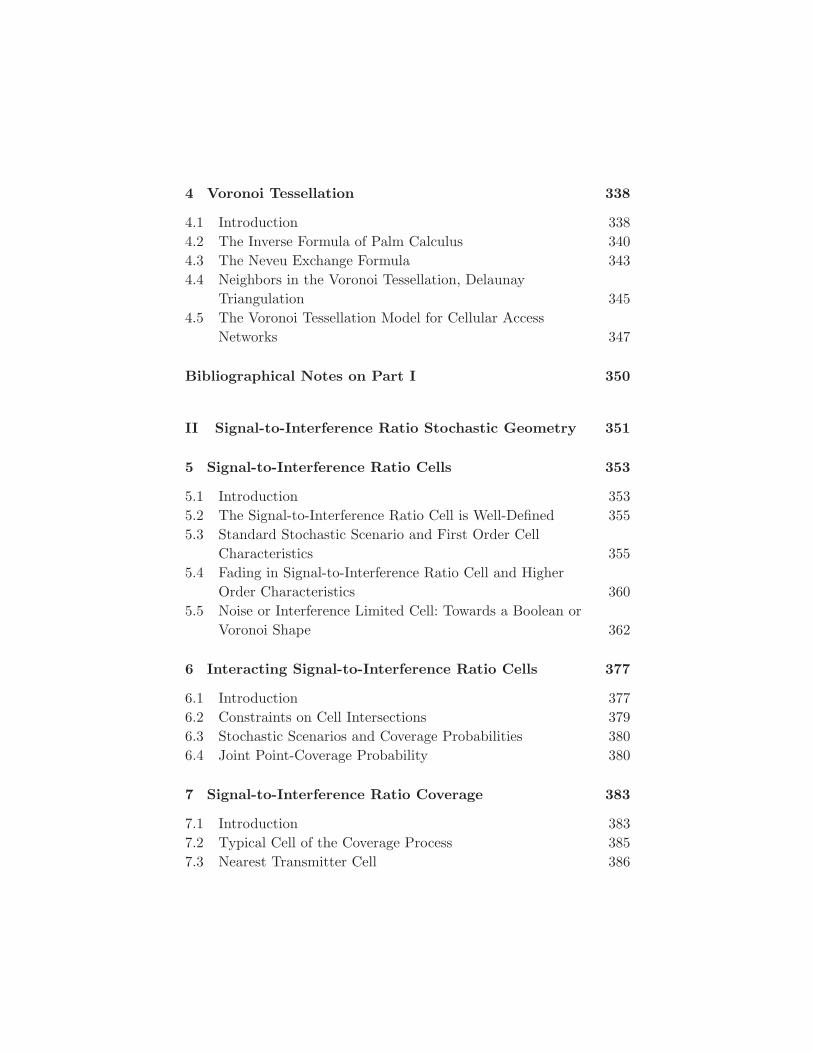
4 Voronoi Tessellation 338
4.1 Introduction 3384.2 The Inverse Formula of Palm Calculus 3404.3 The Neveu Exchange Formula 3434.4 Neighbors in the Voronoi Tessellation, Delaunay
Triangulation 3454.5 The Voronoi Tessellation Model for Cellular Access
Networks 347
Bibliographical Notes on Part I 350
II Signal-to-Interference Ratio Stochastic Geometry 351
5 Signal-to-Interference Ratio Cells 353
5.1 Introduction 3535.2 The Signal-to-Interference Ratio Cell is Well-Defined 3555.3 Standard Stochastic Scenario and First Order Cell
Characteristics 3555.4 Fading in Signal-to-Interference Ratio Cell and Higher
Order Characteristics 3605.5 Noise or Interference Limited Cell: Towards a Boolean or
Voronoi Shape 362
6 Interacting Signal-to-Interference Ratio Cells 377
6.1 Introduction 3776.2 Constraints on Cell Intersections 3796.3 Stochastic Scenarios and Coverage Probabilities 3806.4 Joint Point-Coverage Probability 380
7 Signal-to-Interference Ratio Coverage 383
7.1 Introduction 3837.2 Typical Cell of the Coverage Process 3857.3 Nearest Transmitter Cell 386

7.4 ΞSINR as a Random Closed Set 3887.5 The Coverage Process Characteristics 392
8 Signal-to-Interference Ratio Connectivity 401
8.1 Introduction 4018.2 Signal-to-Interference Ratio Graph 4018.3 Percolation of the Signal-to-Interference Ratio
Connectivity Graph 402
Bibliographical Notes on Part II 410
III Appendix: Mathematical Complements 411
9 Higher Order Moment Measures of aPoint Process 412
9.1 Higher Order Moment Measures 4129.2 Palm Measures 414
10 Stationary Marked Point Processes 417
10.1 Marked Point Processes 41710.2 Palm–Matthes Distribution of a Marked Point Process 418
11 Fairness and Optimality 422
12 Lemmas on Fourier Transforms 424
12.1 Fourier Transforms 42412.2 Lemmas 424
13 Graph Theoretic Notions 429
13.1 Minimum Spanning Tree 429

14 Discrete Percolation 433
14.1 Bond Percolation on Zd. 433
14.2 Independent Site Percolation 437
References 439
Table of Mathematical Notation and Abbreviations 442
Index 445
Foundations and Trends R© inNetworkingVol. 3, Nos. 3-4 (2009) 249–449c© 2009 F. Baccelli and B. Blaszczyszyn
DOI: 10.1561/1300000006
Stochastic Geometry and WirelessNetworks: Volume I Theory
Francois Baccelli1 and Bartlomiej Blaszczyszyn2
1 INRIA & Ecole Normale Superieure, 45 rue d’Ulm, Paris,[email protected]
2 INRIA & Ecole Normale Superieure and Math. Inst. University ofWroclaw, 45 rue d’Ulm, Paris, [email protected]
Abstract
Volume I first provides a compact survey on classical stochastic geome-try models, with a main focus on spatial shot-noise processes, coverageprocesses and random tessellations. It then focuses on signal to inter-ference noise ratio (SINR) stochastic geometry, which is the basis forthe modeling of wireless network protocols and architectures consid-ered in Volume II. It also contains an appendix on mathematical toolsused throughout Stochastic Geometry and Wireless Networks, VolumesI and II.

Preface
A wireless communication network can be viewed as a collection ofnodes, located in some domain, which can in turn be transmitters orreceivers (depending on the network considered, nodes may be mobileusers, base stations in a cellular network, access points of a WiFimesh, etc.). At a given time, several nodes transmit simultaneously,each toward its own receiver. Each transmitter–receiver pair requiresits own wireless link. The signal received from the link transmitter maybe jammed by the signals received from the other transmitters. Evenin the simplest model where the signal power radiated from a pointdecays in an isotropic way with Euclidean distance, the geometry ofthe locations of the nodes plays a key role since it determines the sig-nal to interference and noise ratio (SINR) at each receiver and hencethe possibility of establishing simultaneously this collection of links ata given bit rate. The interference seen by a receiver is the sum of thesignal powers received from all transmitters, except its own transmitter.
Stochastic geometry provides a natural way of defining and com-puting macroscopic properties of such networks, by averaging overall potential geometrical patterns for the nodes, in the same way asqueuing theory provides response times or congestion, averaged overall potential arrival patterns within a given parametric class.
250
Preface 251
Modeling wireless communication networks in terms of stochasticgeometry seems particularly relevant for large scale networks. In thesimplest case, it consists in treating such a network as a snapshot ofa stationary random model in the whole Euclidean plane or space andanalyzing it in a probabilistic way. In particular the locations of thenetwork elements are seen as the realizations of some point processes.When the underlying random model is ergodic, the probabilistic anal-ysis also provides a way of estimating spatial averages which often cap-ture the key dependencies of the network performance characteristics(connectivity, stability, capacity, etc.) as functions of a relatively smallnumber of parameters. Typically, these are the densities of the under-lying point processes and the parameters of the protocols involved.By spatial average, we mean an empirical average made over a largecollection of ‘locations’ in the domain considered; depending on thecases, these locations will simply be certain points of the domain, ornodes located in the domain, or even nodes on a certain route definedon this domain. These various kinds of spatial averages are definedin precise terms in the monograph. This is a very natural approach,e.g. for ad hoc networks, or more generally to describe user positions,when these are best described by random processes. But it can alsobe applied to represent both irregular and regular network architec-tures as observed in cellular wireless networks. In all these cases, sucha space average is performed on a large collection of nodes of the net-work executing some common protocol and considered at some com-mon time when one takes a snapshot of the network. Simple examplesof such averages are the fraction of nodes which transmit, the fractionof space which is covered or connected, the fraction of nodes whichtransmit their packet successfully, and the average geographic progressobtained by a node forwarding a packet towards some destination. Thisis rather new to classical performance evaluation, compared to timeaverages.
Stochastic geometry, which we use as a tool for the evaluation ofsuch spatial averages, is a rich branch of applied probability partic-ularly adapted to the study of random phenomena on the plane orin higher dimension. It is intrinsically related to the theory of pointprocesses. Initially its development was stimulated by applications to

252 Preface
biology, astronomy and material sciences. Nowadays, it is also used inimage analysis and in the context of communication networks. In thislatter case, its role is similar to that played by the theory of pointprocesses on the real line in classical queuing theory.
The use of stochastic geometry for modeling communicationnetworks is relatively new. The first papers appeared in the engineeringliterature shortly before 2000. One can consider Gilbert’s paper of 1961[19] both as the first paper on continuum and Boolean percolation andas the first paper on the analysis of the connectivity of large wirelessnetworks by means of stochastic geometry. Similar observations can bemade on [20] concerning Poisson–Voronoi tessellations. The number ofpapers using some form of stochastic geometry is increasing fast. Oneof the most important observed trends is to take better account in thesemodels of specific mechanisms of wireless communications.
Time averages have been classical objects of performance evaluationsince the work of Erlang (1917). Typical examples include the randomdelay to transmit a packet from a given node, the number of time stepsrequired for a packet to be transported from source to destination onsome multihop route, the frequency with which a transmission is notgranted access due to some capacity limitations, etc. A classical ref-erence on the matter is [28]. These time averages will be studied hereeither on their own or in conjunction with space averages. The combi-nation of the two types of averages unveils interesting new phenomenaand leads to challenging mathematical questions. As we shall see, theorder in which the time and the space averages are performed mattersand each order has a different physical meaning.
This monograph surveys recent results of this approach and is struc-tured in two volumes.
Volume I focuses on the theory of spatial averages and containsthree parts. Part I in Volume I provides a compact survey on classi-cal stochastic geometry models. Part II in Volume I focuses on SINRstochastic geometry. Part III in Volume I is an appendix which containsmathematical tools used throughout the monograph. Volume II bearson more practical wireless network modeling and performance analy-sis. It is in this volume that the interplay between wireless commu-nications and stochastic geometry is deepest and that the time–space

Preface 253
framework alluded to above is the most important. The aim is to showhow stochastic geometry can be used in a more or less systematic wayto analyze the phenomena that arise in this context. Part IV in Vol-ume II is focused on medium access control (MAC). We study MACprotocols used in ad hoc networks and in cellular networks. Part V inVolume II discusses the use of stochastic geometry for the quantita-tive analysis of routing algorithms in MANETs. Part VI in Volume IIgives a concise summary of wireless communication principles and ofthe network architectures considered in the monograph. This part isself-contained and readers not familiar with wireless networking mighteither read it before reading the monograph itself, or refer to it whenneeded.
Here are some comments on what the reader will obtain from study-ing the material contained in this monograph and on possible ways ofreading it.
For readers with a background in applied probability, this mono-graph provides direct access to an emerging and fast growing branchof spatial stochastic modeling (see, e.g., the proceedings of conferencessuch as IEEE Infocom, ACM Sigmetrics, ACM Mobicom, etc. or thespecial issue [22]). By mastering the basic principles of wireless linksand the organization of communications in a wireless network, as sum-marized in Volume II and already alluded to in Volume I, these read-ers will be granted access to a rich field of new questions with highpractical interest. SINR stochastic geometry opens new and interest-ing mathematical questions. The two categories of objects studied inVolume II, namely medium access and routing protocols, have a largenumber of variants and implications. Each of these could give birth to anew stochastic model to be understood and analyzed. Even for classicalmodels of stochastic geometry, the new questions stemming from wire-less networking often provide an original viewpoint. A typical exampleis that of route averages associated with a Poisson point process as dis-cussed in Part V in Volume II. Reader already knowledgeable in basicstochastic geometry might skip Part I in Volume I and follow the path:
Part II in Volume I ⇒ Part IV in Volume II⇒ Part V in Volume II,
254 Preface
using Part VI in Volume II for understanding the physical meaning ofthe examples pertaining to wireless networks.
For readers whose main interest in wireless network design, themonograph aims to offer a new and comprehensive methodology for theperformance evaluation of large scale wireless networks. This methodol-ogy consists in the computation of both time and space averages withina unified setting. This inherently addresses the scalability issue in thatit poses the problems in an infinite domain/population case from thevery beginning. We show that this methodology has the potential toprovide both qualitative and quantitative results as below:
• Some of the most important qualitative results pertainingto these infinite population models are in terms of phasetransitions. A typical example bears on the conditions underwhich the network is spatially connected. Another type ofphase transition bears on the conditions under which thenetwork delivers packets in a finite mean time for a givenmedium access and a given routing protocol. As we shall see,these phase transitions allow one to understand how to tunethe protocol parameters to ensure that the network is in thedesirable “phase” (i.e. well connected and with small meandelays). Other qualitative results are in terms of scaling laws:for instance, how do the overhead or the end-to-end delay ona route scale with the distance between the source and thedestination, or with the density of nodes?
• Quantitative results are often in terms of closed form expres-sions for both time and space averages, and this for eachvariant of the involved protocols. The reader will hence bein a position to discuss and compare various protocols andmore generally various wireless network organizations. Hereare typical questions addressed and answered in Volume II:is it better to improve on Aloha by using a collision avoid-ance scheme of the CSMA type or by using a channel-awareextension of Aloha? Is Rayleigh fading beneficial or detri-mental when using a given MAC scheme? How does geo-graphic routing compare to shortest path routing in a mobile

Preface 255
ad hoc network? Is it better to separate the medium accessand the routing decisions or to perform some cross layer jointoptimization?
The reader with a wireless communication background could eitherread the monograph from beginning to end, or start with Volume II,i.e. follow the path
Part IV in Volume II ⇒ Part V in Volume II ⇒ Part II in Volume I
and use Volume I when needed to find the mathematical results whichare needed to progress through Volume II.
We conclude with some comments on what the reader will not findin this monograph:
• We do not discuss statistical questions and give no measure-ment based validation of certain stochastic assumptions usedin the monograph, e.g., when are Poisson-based models justi-fied? When should one rather use point processes with somerepulsion or attraction? When is the stationarity/ergodicityassumption valid? Our only aim is to show what can be donewith stochastic geometry when assumptions of this kind canbe made.
• We will not go beyond SINR models either. It is well knownthat considering interference as noise is not the only possibleoption in a wireless network. Other options (collaborativeschemes, successive cancellation techniques) can offer betterrates, though at the expense of more algorithmic overheadand the exchange of more information between nodes. Webelieve that the methodology discussed in this monographhas the potential of analyzing such techniques but we decidednot to do this here.
Here are some final technical remarks. Some sections, marked witha * sign, can be skipped at the first reading as their results are notused in what follows; the index, which is common to the two volumes,is designed to be the main tool to navigate within and between the twovolumes.

256 Preface
Acknowledgments
The authors would like to express their gratitude to Dietrich Stoyan,who first suggested them to write a monograph on this topic, aswell as to Daryl Daley and Martin Haenggi for their very valuableproof-reading of the manuscript. They would also like to thank theanonymous reviewer of NOW for his/her suggestions, particularly soconcerning the two volume format, as well as Paola Bermolen, PierreBremaud, Srikant Iyer, Mohamed Karray, Omid Mirsadeghi, Paul Muh-lethaler, Barbara Staehle and Patrick Thiran for their useful commentson the manuscript.

Preface to Volume I
This volume focuses on the theory and contains three parts.Part I provides a compact survey on classical stochastic geometry
models. The basic models defined in this part will be used and extendedthroughout the whole monograph, and in particular to SINR basedmodels. Note, however, that these classical stochastic models can beused in a variety of contexts which go far beyond the modeling ofwireless networks. Chapter 1 reviews the definition and basic propertiesof Poisson point processes in Euclidean space. We review key operationson Poisson point processes (thinning, superposition, displacement) aswell as key formulas like Campbell’s formula. Chapter 2 is focused onproperties of the spatial shot-noise process: its continuity properties,Laplace transform, moments, etc. Both additive and max shot-noiseprocesses are studied. Chapter 3 bears on coverage processes, and inparticular on the Boolean model. Its basic coverage characteristics arereviewed. We also give a brief account of its percolation properties.Chapter 4 studies random tessellations; the main focus is on Poisson–Voronoi tessellations and cells. We also discuss various random objectsassociated with bivariate point processes such as the set of points of
257
258 Preface to Volume I
the first point process that fall in a Voronoi cell w.r.t. the second pointprocess.
Part II focuses on the stochastic geometry of SINR. The key newstochastic geometry model can be described as follows: consider amarked point process of the Euclidean space, where the mark of a pointis a positive random variable that represents its “transmission power”.The SINR cell of a point is then defined as the region of the spacewhere the reception power from this point is larger than an affine func-tion of the interference power. Chapter 5 analyzes a few basic stochas-tic geometry questions pertaining to such SINR cells in the case withindependent marks, such as the volume and the shape of the typicalcell. Chapter 6 focuses on the complex interactions that exist betweencells. Chapter 7 studies the coverage process created by the collectionof SINR cells. Chapter 8 studies the impact of interferences on the con-nectivity of large-scale mobile ad hoc networks using percolation theoryon the SINR graph.
Part III is an appendix which contains mathematical tools usedthroughout the monograph.
It was our choice not to cover Gibbs point processes and the randomclosed sets that one can associate to them. And this in spite of the factthat these point processes already seem to be quite relevant withinthis wireless network context (see the bibliography of Chapter 18 inVolume II for instance). There are two main reasons for this decision:first, these models are rarely amenable to closed form analysis, at leastin the case of systems with randomly located nodes as those consideredhere; second and more importantly, the amount of additional materialneeded to cover this part of the theory is not compatible with theformat retained here.

Part I
Classical StochasticGeometry

260
The most basic objects studied in classical stochastic geometry aremultidimensional point processes, which are covered in Chapter 1, witha special emphasis on the most prominent one, the Poisson point pro-cess. Our default observation space in this part will be the Euclideanspace R
d of dimension d ≥ 1. Even if for most of the applications stud-ied later, the plane R
2 (2D) suffices, it is convenient to formulate someresults in 3D or 4D (e. g., to consider time and space).
Shot noise fields, which are used quite naturally to represent inter-ference fields, are studied in Chapter 2. Chapter 3 is focused on coverageprocesses, with the particularly important special case of the Booleanmodel. Chapter 4 bears on Voronoi tessellations and Delaunay graphs,which are useful in a variety of contexts in wireless network modeling.These basic tools will be needed for analyzing the SINR models stem-ming from wireless communications to be analyzed from Part II on.They will be instrumental for analyzing spatio-temporal models whencombined with Markov process techniques.

1Poisson Point Process
Consider the d -dimensional Euclidean space Rd. A spatial point process
(p.p.)Φ is a random, finite or countably-infinite collection of points inthe space R
d, without accumulation points.One can consider any given realization φ of a point process as a
discrete subset φ = xi ⊂ Rd of the space. It is often more convenient
to think of φ as a counting measure or a point measure φ =∑
i εxi
where εx is the Dirac measure at x; for A ⊂ Rd, εx(A) = 1 if x ∈ A and
εx(A) = 0 if x ∈ A. Consequently, φ(A) gives the number of “points” ofφ in A. Also, for all real functions f defined on R
d, we have∑
i f(xi) =∫Rd f(x)φ(dx). We will denote by M the set of all point measures that
do not have accumulation points in Rd. This means that any φ ∈ M
is locally finite, that is φ(A) < ∞ for any bounded A ⊂ Rd (a set is
bounded if it is contained in a ball with finite radius).Note that a p.p. Φ can be seen as a stochastic process Φ =
Φ(A)A∈B with state space N = 0,1, . . . Φ(A) and where the indexA runs over bounded Borel subsets of R
d. Moreover, as for “usual”stochastic processes, the distribution of a p.p. is entirely characterized
261
262 Poisson Point Process
by the family of finite dimensional distributions (Φ(A1), . . . ,Φ(Ak)),where A1, . . . ,Ak run over the bounded subsets of R
d.1
1.1 Definition and Characterizations
1.1.1 Definition
Let Λ be a locally finite non-null measure on Rd.
Definition 1.1. The Poisson point process Φ of intensity measure Λis defined by means of its finite-dimensional distributions:
PΦ(A1) = n1, . . . ,Φ(Ak) = nk =k∏
i=1
(e−Λ(Ai) Λ(Ai)ni
ni!
),
for every k = 1,2, . . . and all bounded, mutually disjoint sets Ai fori = 1, . . . ,k. If Λ(dx) = λ dx is a multiple of Lebesgue measure (volume)in R
d, we call Φ a homogeneous Poisson p.p. and λ is its intensityparameter.
It is not evident that such a point process exists. Later, we will showhow it can be constructed. Suppose for the moment that it does exist.Here are a few immediate observations made directly from the abovedefinition:
• Φ is a Poisson p.p., if and only if for every k = 1,2, . . .
and all bounded, mutually disjoint Ai ⊂ Rd for i = 1, . . . ,k,
(Φ(A1), . . . ,Φ(Ak)) is a vector of independent Poisson ran-dom variables of parameter Λ(Ai), . . . ,Λ(Ak), respectively. Inparticular, E(Φ(A)) = Λ(A), for all A.
• Let W be some bounded observation window and letA1, . . . ,Ak be some partition of this window: Ai ∩ Aj = ∅ for
1 We do not discuss here the measure-theoretic foundations of p.p. theory; we remark thateach time we talk about a subset B of R
d or a function f defined on Rd, we understand that
they belong to some “nice class of subsets that can be measured” and to some “nice classof functions that can be integrated”. A similar convention is assumed for subsets of M andfunctions defined on this space (typically, we want all events of the type µ ∈ M:µ(A) = k,A ⊂ R
d, k ∈ N, to be ”measurable”). See [9] or [10], [11] for details.

1.1 Definition and Characterizations 263
j = i and⋃
i Ai = W . For all n,n1, . . . ,nk ∈ N with∑
i ni = n,
PΦ(A1) = n1, . . . ,Φ(Ak) = nk | Φ(W ) = n=
n!n1! . . .nk!
1Λ(W )n
∏i
Λ(Ai)ni . (1.1)
The above conditional distribution is the multinomial dis-tribution. This last property shows that given there are n
points in the window W , these points are independentlyand identically distributed (i.i.d.) in W according to the lawΛ(·)/Λ(W ).
Example 1.1 (Locations of nodes in ad hoc networks). Assumethat nodes (users), who are supposed to constitute an ad hoc network(see Section 25.3.1 in Volume II), arrive at some given region W (asubset of the plane or the 3D space) and independently take their loca-tions in W at random according to some probability distribution a(·).This means that each user chooses location dx with probability a(dx);the uniform distribution corresponds to a “homogeneous” situation andnon-uniform distributions allow us to model, e.g., various “hot spots”.Then, in view of what was said above, the configuration of n users ofthis ad hoc network coincides in law with the conditional distributionof the Poisson p.p. Φ with intensity Λ(dx) proportional to a(dx) on W ,given Φ(W ) = n.
Suppose now that one does not want to fix a priori the exact num-ber of nodes in the network, but only the “average” number A(dx)of nodes per dx is known. In such a situation it is natural to assumethat the locations of nodes in W are modeled by the atoms of the(non-conditioned) Poisson process with intensity Λ(dx) = A(dx).2
The observation about conditional distribution suggests a first con-struction of the Poisson p.p. in a bounded window; sample a Poisson
2 One can make the story of nodes arriving to W more complete. Assuming a spatio-temporalPoisson arrival process of nodes, independent Markovian mobility of each node and inde-pendent exponential sojourn time of each node in the network before its departure oneobtains a spatial birth-and-death process with migrations, who has Poisson p.p. as itsstationary (in time) distribution; see [41, Section 9]
264 Poisson Point Process
random variable of parameter Λ(W ) and if the outcome is n, sample n
i.i.d. random variables with distribution Λ(·)/Λ(W ) on W . The exten-sion of the construction to the whole space R
d can then be done byconsidering a countable partition of R
d into bounded windows and anindependent generation of the Poisson p.p. in each window. We willreturn to this idea in Section 1.2. Before this, we give more terminol-ogy and other characterizations of the Poisson p.p.
1.1.2 Characterizations by the Form of the Distribution
• Say that Φ has a fixed atom at x0 if PΦ(x0) > 0 > 0.• Call a p.p. Φ simple if PΦ(x) = 0 or 1 for all x = 1; i.e.,
if with probability 1, Φ =∑
i εxi , where the points xi arepairwise different.
Proposition 1.1. Let Φ be a Poisson p.p. with intensity measure Λ.
• Φ has a fixed atom at x0 if and only if Λ has an atom atx0 ∈ R
d (i.e. Λ(x0) > 0).• A Poisson p.p. Φ is simple if Λ is non-atomic, i.e. admits a
density with respect to Lebesgue measure in Rd.
Proof. The first part is easy: use Definition 1.1 to write PΦ(x0) >
0 = 1 − e−Λ(x0) > 0 if and only if Λ(x0) > 0.The second part can be proved using the conditioning (1.1) along
the following lines. Let us take a bounded subset A ⊂ Rd.
PΦ is simple in A
=∞∑
n=2
PΦ(A) = nPall n points of Φ are different | Φ(A) = n
=∞∑
n=2
e−Λ(A) (Λ(A))n
n!1
(Λ(A))n
×∫
A· · ·∫
A(xj all different)Λ(dx1) · · ·Λ(dxn) = 1.
1.1 Definition and Characterizations 265
We conclude the proof that PΦ is simple = 1 by considering anincreasing sequence of bounded sets Ak R
d and using the monotoneconvergence theorem.
We now give two characterizations of the Poisson p.p. based on theform of the distribution of the variable Φ(A) for all A.
Theorem 1.2. Φ is a Poisson p.p. if and only if there exists a locallyfinite measure Λ on R
d such that for all bounded A, Φ(A) is a Poissonrandom variable (r. v. ) with parameter Λ(A).
Proof. We use the following fact that can be proved using momentgenerating functions (cf. Daley and Vere-Jones, [9], Lemma 2.3.I):suppose (X,X1, . . . ,Xn) is a random vector with Poisson marginal dis-tributions and such that X =
∑ni=1 Xi; then X1, . . . ,Xn are mutually
independent.
Theorem 1.3. Suppose that Φ is a simple p.p. Then Φ is a Poissonp.p. if and only if there exists a locally finite non-atomic measure Λsuch that for any subset A, PΦ(A) = 0 = e−Λ(A).
Proof. This is a consequence of a more general result saying that thedistribution of the p.p. is completely defined by its void probabilities;see ([27], Th. 3.3) for more details.
1.1.3 Characterization by Complete Independence
Definition 1.2. One says that the p.p. Φ has the property of com-plete independence if for any finite family of bounded subsets A1, . . . ,Ak
that are mutually disjoint, the random variables Φ(A1), . . . ,Φ(Ak) areindependent.
266 Poisson Point Process
Theorem 1.4. Suppose that Φ is a p.p. without fixed atoms. Then Φis a Poisson p.p. if and only if
(1) Φ is simple, and(2) Φ has the property of complete independence.
Proof. The necessity follows from Proposition 1.1. For sufficiency,one shows that the measure Λ(A) = − log(PΦ(A) = 0) satisfies theassumptions of Theorem 1.3. (cf. [27], Section 2.1).
1.2 Laplace Functional
Definition 1.3. The Laplace functional L of a p.p. Φ is defined by thefollowing formula
LΦ(f) = E[e−∫
Rd f(x)Φ(dx)],where f runs over the set of all non-negative functions on R
d.
Note that the Laplace functional completely characterizes the distribu-tion of the p.p. Indeed, for f(x) =
∑ki=1 ti (x ∈ Ai),
LΦ(f) = E[e−∑
i tiΦ(Ai)],
seen as a function of the vector (t1, . . . , tk), is the joint Laplace transformof the random vector (Φ(A1), . . . ,Φ(Ak)), whose distribution is charac-terized by this transform. When A1, . . . ,Ak run over all bounded sub-sets of the space, one obtains a characterization of all finite-dimensionaldistributions of the p.p.
Here is a very useful characterization of the Poisson p.p. by itsLaplace functional.
Proposition 1.5. The Laplace functional of the Poisson p.p. of inten-sity measure Λ is
LΦ(f) = e−∫Rd (1−e−f(x))Λ(dx). (1.2)
1.2 Laplace Functional 267
Proof. For a given non-negative function f(x), consider the functiong(x) = f(x) (x ∈ A), where A ∈ B is bounded. We have
LΦ(g) = e−Λ(A)∞∑
n=0
(Λ(A))n
n!1
(Λ(A))n
×∫
A· · ·∫
Ae−∑n
i=1 f(xi) Λ(dx1) · · ·Λ(dxn)
= e−Λ(A)∞∑
n=0
1n!
(∫A
e−f(x) Λ(dx))n
= e−∫Rd (1−e−g(x))Λ(dx).
We conclude the proof by considering an increasing sequenceof bounded sets Ak R
d and using the monotone convergencetheorem.
Taking f(x) = sg(x) with s ≥ 0 and with g(·) ≥ 0 in (1.2) and differen-tiating w.r.t. s at s = 0, we get the following corollary:
E∫
Rd
f(x)Φ(dx) =∫
Rd
f(x)Λ(dx). (1.3)
Construction of the Poisson p.p. in a Bounded Window.Given an intensity measure Λ and a bounded subset W of the space,consider the following independent random objects N,X1,X2, . . .,where
• N is a Poisson r. v. with parameter Λ(W ),• X1,X2, . . . are identically distributed random vectors (points)
taking values in W ⊂ Rd with PX1 ∈ · = Λ(·)/Λ(W ).
In connection with the remark at the end of Section 1.1.1, we showbelow using Laplace functionals that Φ =
∑Nk=1 εXi is a Poisson p.p.
with intensity measure Λ|W (·) = Λ(· ∩ W ), the restriction of Λ to W .Evidently Φ is a random set of points in W . We now calculate the

268 Poisson Point Process
Laplace functional of Φ. For a non-negative function f , we have
LΦ(f) = E[
(N = 0) + (N > 0)e−∑Nk=1 f(Xi)
]= e−Λ(W )
∞∑k=0
(Λ(W ))k
k!
(∫W
e−f(x) Λ(dx)Λ(W )
)k
= e−Λ(W )+∫
W e−f(x) Λ(dx)
= e−∫W (1−e−f(x))Λ(dx),
which shows that Φ is the announced Poisson p.p. The above construc-tion can be extended to the whole space. We will do it in the nextsection.
In the following example, we show that Definition 1.1 for d = 1, i.e.of a Poisson p.p. in 1D, is equivalent to frequently used definition basedon independent, exponentially distributed inter-point distances.
Example 1.2 (Homogeneous Poisson p.p. in 1D). Consider aPoisson p.p. Φ =
∑k εSk
on the real line R with intensity measure λdx,where 0 < λ < ∞. Assume that the atoms of Φ are numbered in sucha way that Sk−1 < Sk for k ∈ Z (by Proposition 1.1 the atoms of Φare pairwise different) and S1 = maxx > 0:Φ((0,x)) = 0 is the firstatom of Φ in the open positive half-line (0,∞). We will show thatSk can be constructed as a renewal process with exponential hold-ing times, i.e., Sk =
∑ki=1 Fi for k ≥ 1 and Sk = −∑0
i=k Fi for k ≤ 0,where Fk : k = . . . ,−1,0,1 . . . is a sequence of independent, identi-cally distributed exponential random variables. Indeed, PF1 > t =PS1 > t = PΦ((0, t]) = 0 = e−λt so S1 = F1 is exponential randomvariable with parameter λ. By the the strong Markov property (Propo-sition 1.16), for all k ≥ 2,
PFk > t | F1, . . . ,Fk−1 = PSk − Sk−1 > t | S1, . . . ,Sk−1= PSk − Sk−1 > t | Sk−1= PΦ((Sk−1,Sk−1 + t]) = 0 | Sk−1= e−λt
and similarly for k ≤ 0, with Fkk≤0 and Fkk≥1 being independent.
1.3 Operations Preserving the Poisson Law 269
Remark. In the last example, we have evaluated the probabilitiesof the events of the form S1 > t, Sk − Sk−1 > t. This was doneunder the tacit assumption that in the representation Φ =
∑k εSk
,the variables Sk are random variables, i.e., that the correspondingevents belong to the “nice class” of events whose probabilities can bemeasured. This is true in this particular case and, more generally, pointsof any p.p. Φ can always be numbered in such a way that the locationof the point with a given number is a random variable (see Kallenberg,[27]). In what follows, we assume that xk are random variables anytime we use a representation of the form Φ =
∑k εxk
.
1.3 Operations Preserving the Poisson Law
1.3.1 Superposition
Definition 1.4. The superposition of point processes Φk is defined asthe sum Φ =
∑k Φk.
Note that the summation in the above definition is understood as thesummation of (point) measures. It always defines a point measure,which however, in general, might not be locally finite (we do not assumethe last sum to have finitely many terms). Here is a very crude, butuseful condition for this to not happen.
Lemma 1.6. The superposition Φ =∑
k Φk is a p.p. if∑
k E[Φk(·)] isa locally finite measure.
A refined sufficient condition may be found by the Borel–Cantellilemma.
Proposition 1.7. The superposition of independent Poisson pointprocesses with intensities Λk is a Poisson p.p. with intensity measure∑
k Λk if and only if the latter is a locally finite measure.
Proof. ⇒ By the definition.⇐ By Lemma 1.6 the superposition is a p.p. One evaluates its Laplace

270 Poisson Point Process
functional as follows
E[e−∑
k
∫Rd f(x)Φk(dx)] = E
[∏k
e−∫Rd f(x)Φk(dx)
]=∏k
e−∫Rd (1−e−f(x))Λk(dx)
= e−∫Rd (1−e−f(x))(
∑k Λk(dx)).
Construction of Poisson p.p. on the Whole Space. We return tothe construction of the Poisson p.p. with given intensity measure Λ. LetWkk=1,... be a countable partition of the space with Wk bounded forall k. Following the arguments described in Section 1.1.1, we constructin each Wk an independent copy of the Poisson p.p. with intensitymeasure Λk(·) = Λ(· ∩ Wk). By Proposition 1.7, Φ =
∑k Φk is a Poisson
p.p. of intensity measure Λ =∑
k Λk.
1.3.2 Thinning
Consider a function p:Rd → [0,1] and a p.p. Φ.
Definition 1.5. The thinning of Φ with the retention function p is ap.p. given by
Φp =∑
k
δkεxk, (1.4)
where the random variables δkk are independent given Φ, and Pδk =1 | Φ = 1 − Pδk = 0 | Φ = p(xk).
Less formally, we can say that a realization of Φp can be constructedfrom that of Φ by randomly and independently removing some fractionof points; the probability that a given point of Φ located at x is notremoved (i.e. is retained in Φp) is equal to p(x).
It is not difficult to verify that the above construction transforms aPoisson p.p. into another Poisson p.p.
1.3 Operations Preserving the Poisson Law 271
Proposition 1.8. The thinning of the Poisson p.p. of intensity mea-sure Λ with the retention probability p yields a Poisson p.p. of intensitymeasure pΛ with (pΛ)(A) =
∫A p(x)Λ(dx).
Proof. The Laplace functional of Φp at g = f1A with A bounded is
LΦp(g) = e−Λ(A)∞∑
n=0
(Λ(A))n
n!1
(Λ(A))n
×∫
A· · ·∫
A
n∏i=1
(p(xi)e−f(xi) + 1 − p(xi)
)Λ(dx1) . . .Λ(dxn)
= e−Λ(A)∞∑
n=0
1n!
(∫A
(p(x)e−f(x) + 1 − p(x)
)Λ(dx)
)n
= e−∫Rd (1−e−g(x))p(x)Λ(dx).
Example 1.3 (Aloha). A typical application is that of some ad hocnetwork made of nodes distributed according to some Poisson pointprocess and using Aloha as medium access control (see Section 25.1.2in Volume II). The principle of this protocol is that each node tosses acoin independently of everything else to decide whether it accesses theshared wireless medium or not. The bias of this coin may depend on thelocal density of nodes. The last result shows that the set of transmittersis a Poisson p.p. The set of nodes which refrain transmitting is alsoPoisson.
Corollary 1.9. The restriction Φ|W of a Poisson p.p. of intensity mea-sure Λ to some given set W is a Poisson p.p. with intensity measureΛ(· ∩ W ) = Λ|W (· · ·).
1.3.3 Random Transformation of Points
Consider a probability kernel p(x,B) from Rd to R
d′, where d′ ≥ 1, i.e.
for all x ∈ Rd, p(x, ·) is a probability measure on R
d′.

272 Poisson Point Process
Definition 1.6. The transformation Φp of a p.p. Φ by a probabilitykernel p(·, ·) is a point process in R
d′given by
Φp =∑
k
εyk, (1.5)
where the Rd′
-valued random vectors ykk are independent given Φ,with Pyk ∈ B′ | Φ = p(xk,B
′).3
In other words, Φp is obtained by randomly and independentlydisplacing each point of Φ from R
d to some new location in Rd′
accord-ing to the kernel p. This operation preserves the Poisson p.p. propertyas stated in the following theorem.
Theorem 1.10 (Displacement Theorem). The transformation ofthe Poisson p.p. of intensity measure Λ by a probability kernel p is thePoisson p.p. with intensity measure Λ′(A) =
∫Rd p(x,A)Λ(dx), A ⊂ R
d′.
Proof. The Laplace functional of Φp is
LΦp(f) = Eexp
[−∑
i
f(Yi)
]
= E∫
Rd′. . .
∫Rd′
e−∑i f(yi)
∏j
p(Xj ,dyj)
= E∏j
∫yj∈Rd′
e−f(yj)p(Xj ,dyj)
= Eexp
∑j
log(∫
y∈Rd′e−f(y)p(Xj ,dy)
) .
3 We use the same notation Φp for the p-thinning and the transformation by kernel p. Thecontext indicates what is meant.

1.3 Operations Preserving the Poisson Law 273
Evaluating now the Laplace functional of Φ at g with g(x) =− log
(∫y∈Rd′ e−f(y)p(x,dy)
), we get
LΦp(f) = LΦ(g) = exp[−∫
Rd
(1 − elog
∫Rd′ e−f(y) p(x,dy)
)Λ(dx)
]= exp
[−∫
Rd
(1 −
∫Rd′
e−f(y) p(x,dy))
Λ(dx)]
= exp[−∫
Rd
∫Rd′
(1 − e−f(y))p(x,dy)Λ(dx)]
= exp[−∫
Rd′(1 − e−f(y))Λ′(dy)
].
Example 1.4 (Random walk and random waypoint mobility).Consider some Mobile Ad hoc NETwork (MANET) — see Sec-tion 25.3.1 in Volume II. Assume the MANET nodes to be initiallydistributed according to some Poisson p.p. Assume each node thenmoves according to some discrete time, continuous state space Markovchain with kernel p(x,dy) on R
d. More precisely, at each time slot,each node is displaced from its initial position x ∈ R
d to a new positiony ∈ R
d, independently of everything else. The displacement is randomand its law depends only on x.
The last result shows that the displaced points still form a Poissonp.p. The joint Laplace functional of Φ = Xi (the initial p.p.) and Φ′ =Yi (the displaced p.p.) at f,g, where f and g are positive functions,is defined as
LΦ,Φ′(f,g) = E(e−∑
i f(Xi)−∑
i g(Yi)).
Using arguments similar to those in the last proof, one gets that
LΦ,Φ′(f,g) = exp[−∫
Rd
(1 −
∫Rd
e−f(x)−g(y) p(x,dy))
Λ(dx)]
= exp[−∫
Rd
(1 − e−g(y))Λ′(dy)]
×exp[−∫
Rd
(1 − e−f(x))(∫
Rd
e−g(y) p(x,dy))
Λ(dx)].
274 Poisson Point Process
This displacement scheme can of course be iterated further while pre-serving the Poisson property.
Notice that if the initial Poisson p.p. has an intensity measure whichis 0 outside a finite window W , one can use this Markov model to‘maintain’ all displaced points in W by appropriate choices of the dis-placement laws.
Here are a few particular cases of this general model:
• The random walk model is that where the displacement con-sists in adding to x an independent random variable D withsome fixed law H on R
d \ 0 which does not depend on x.• The random waypoint model is similar to the latter, but with
the displacement equal to 0 with probability π and to a non-null random vector with a fixed distribution H on R
d \ 0with probability 1 − π. A node either ‘stops’ with probabilityπ or moves in some new direction with the complementaryprobability.
• The high mobility random walk case features a small param-eter ε > 0 and consists in adding the random variable D/ε tox to get the new position; here, the law of D is as in the firstcase above. Then
LΦ,Φ′(f,g) = LΦ′(g)exp[−∫
Rd
(1 − e−f(x))
×(∫
Rd\0e−g(x+y/ε)H(dy)
)Λ(dx)
].
Let us show how to use this formula to prove that for homo-geneous Poisson p.p., this high mobility case leads to inde-pendence between Φ and Φ′ when ε → 0. For this, it is enoughto prove that for all functions g which tend to 0 at infinityin all directions,
limε→∞
∫Rd
(1 − e−f(x))
(∫Rd\0
e−g(x+y/ε)H(dy)
)dx
=∫
Rd
(1 − e−f(x))dx.

1.3 Operations Preserving the Poisson Law 275
But for all x and all y = 0, g(x + y/ε) tends to 0 when ε tendsto 0. This and the dominated convergence theorem allow oneto conclude the proof of independence.Notice that this independence property does not hold in thehigh mobility random waypoint model as defined above.
Example 1.5 (Transformation of space). Consider a functionG:Rd → R
d′. Note that the mapping G can be seen as a special case of a
probability kernel from one space to the other, which transforms x ∈ Rd
into G(x) with probability 1. Suppose Φ is a Poisson p.p. with intensitymeasure Λ on R
d. By Theorem 1.10, Φ′ =∑
k εG(xk) is a Poisson p.p.on R
d′with intensity measure Λ′(·) = Λ(G−1(·)).
Example 1.6(Dilation). A special case of a transformation Rd onto
itself is a dilation by a given factor γ: G(x) = γx, x ∈ Rd. By the above
result Φ′ =∑
k εγxkis a Poisson p.p. with intensity measure Λ′(A) =
Λ(A/γ), where A/γ = y/γ:y ∈ A.
Example 1.7 (Homogenization). Another special case consists infinding some transformation G which makes of Φ′ a homogeneous Pois-son p.p. For this, assume that Λ(dx) = λ(x)dx and suppose that G(x)is a differentiable mapping from R
d to Rd, which satisfies the functional
equation on Rd given by
λ(x) = λ |JG(x)|,where λ is some constant and JG is the Jacobian of G. Then, note thatfor all A ⊂ R
d
Λ(G−1(A)) =∫
G−1(A)λ(x)dx =
∫G−1(A)
λ|JG(x)|dx =∫
Aλdx,
which proves that the intensity measure of Φ′ is Λ′(dx) = λdx;see (Senoussi et al., [40]) for more details. In particular in 1D (d = 1),

276 Poisson Point Process
the function G(t) =∫ t
0 λ(s)ds transforms the inhomogeneous Poissonp.p. on [0,∞) into the homogeneous one of intensity (parameter) 1 on[0,∞). This construction can easily be extended to R by consideringthe analogous transformation on the negative half-line.
Example 1.8 (Polar coordinates). Consider a homogeneous Pois-son p.p. Φ on R
2 with constant intensity λ and let G(x):R2 → R+ ×
[0,2π) be the mapping G(x) = (|x|,∠(x)), where ∠(x) is the argumentof x) (i. e., the angle between vector x and the X axis). Then the trans-formation Φ′ of Φ by G(x) is a Poisson p.p. with intensity measure
Λ′([0, r), [0,θ))
= λπr2θ/(2π), r ≥ 0, 0 ≤ θ < 2π.
The point process Φ′ can also be seen as Poisson p.p. on [0,∞) withintensity measure ΛT (dt) = λπt2, independently marked in the space[0,2π), with uniform mark distribution (cf. Section 2.1).
1.4 Palm Theory
Palm theory formalizes the notion of the conditional distribution ofa general p.p. given it has a point at some location. Note that for ap.p. without a fixed atom at this particular location, the probabilityof the condition is equal to 0 and the basic discrete definition of theconditional probability does not apply. In this section, we will outlinethe definition based on the Radon–Nikodym theorem.
We first define two measures associated with a general point process:
Definition 1.7. The mean measure of a p.p. Φ is the measure
M(A) = E[Φ(A)] (1.6)
on Rd. The reduced Campbell measure of Φ is the measure
C !(A × Γ) = E[∫
A(Φ − εx ∈ Γ)Φ(dx)
](1.7)
on Rd × M, where M denotes the set of point measures.
1.4 Palm Theory 277
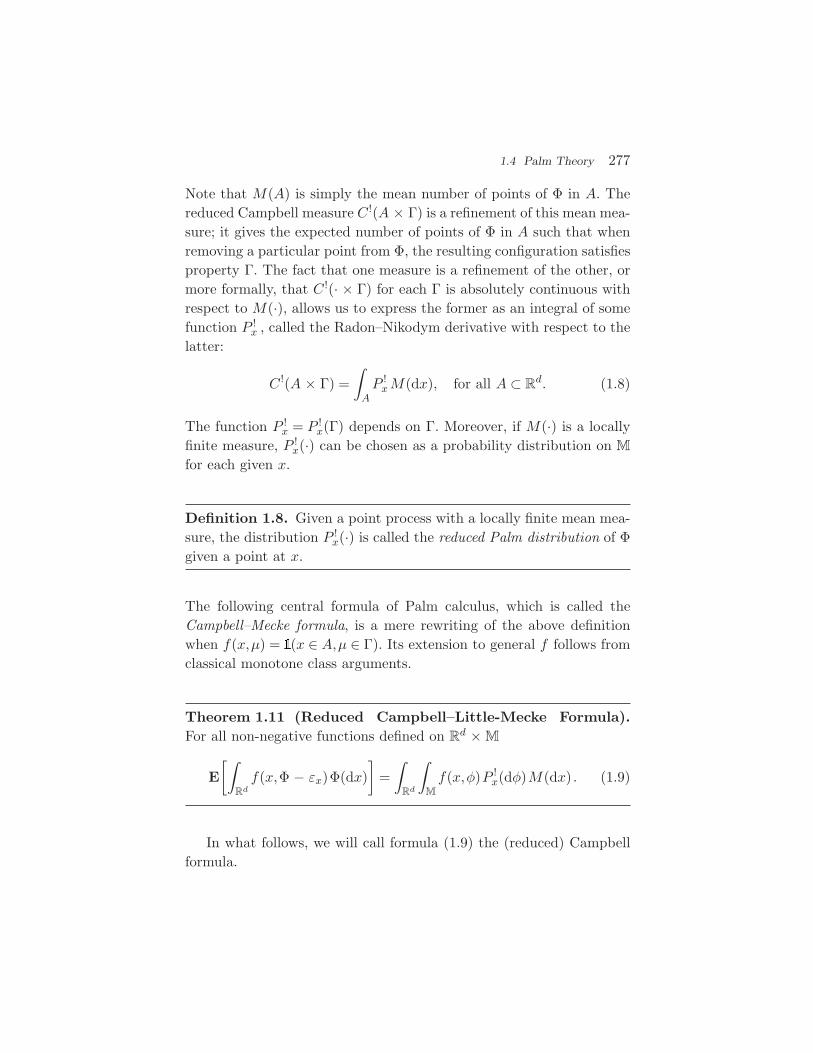
Note that M(A) is simply the mean number of points of Φ in A. Thereduced Campbell measure C !(A × Γ) is a refinement of this mean mea-sure; it gives the expected number of points of Φ in A such that whenremoving a particular point from Φ, the resulting configuration satisfiesproperty Γ. The fact that one measure is a refinement of the other, ormore formally, that C !(· × Γ) for each Γ is absolutely continuous withrespect to M(·), allows us to express the former as an integral of somefunction P !
x , called the Radon–Nikodym derivative with respect to thelatter:
C !(A × Γ) =∫
AP !
x M(dx), for all A ⊂ Rd. (1.8)
The function P !x = P !
x(Γ) depends on Γ. Moreover, if M(·) is a locallyfinite measure, P !
x(·) can be chosen as a probability distribution on M
for each given x.
Definition 1.8. Given a point process with a locally finite mean mea-sure, the distribution P !
x(·) is called the reduced Palm distribution of Φgiven a point at x.
The following central formula of Palm calculus, which is called theCampbell–Mecke formula, is a mere rewriting of the above definitionwhen f(x,µ) = (x ∈ A,µ ∈ Γ). Its extension to general f follows fromclassical monotone class arguments.
Theorem 1.11 (Reduced Campbell–Little-Mecke Formula).For all non-negative functions defined on R
d × M
E[∫
Rd
f(x,Φ − εx)Φ(dx)]
=∫
Rd
∫M
f(x,φ)P !x(dφ)M(dx) . (1.9)
In what follows, we will call formula (1.9) the (reduced) Campbellformula.

278 Poisson Point Process
One can define the (non-reduced) Campbell measure by replacing(Φ ∈ Γ − εx) by (Φ ∈ Γ) in (1.8), i.e.,
C(A × Γ) = E[∫
A(Φ ∈ Γ)Φ(dx)
]
= E
[∑i
(xi ∈ A) (Φ ∈ Γ)
]= E[Φ(A) (Φ ∈ Γ)]. (1.10)
This leads to a (non-reduced) Palm measure Px which can also bedefined by
Px(Γ) = P !x(φ : φ + εx ∈ Γ).
We call Px the Palm distribution of Φ.Taking f(x,φ) = g(x,φ + εx) and substituting in (1.9), we obtain
the following (non-reduced) version of Campbell’s formula:
E[∫
Rd
g(x,Φ)Φ(dx)]
=∫
Rd
∫M
g(x,φ)Px(dφ)M(dx) . (1.11)
We now focus on Poisson point processes. Directly from Defini-tion 1.1, we have:
Corollary 1.12. The mean measure of a Poisson p.p. is equal to itsintensity measure M(·) = Λ(·).
We now state a central result of the Palm theory for Poisson p.p. Itmakes clear why the reduced Palm distributions are more convenientin many situations.
Theorem 1.13 (Slivnyak–Mecke Theorem). Let Φ be a Poissonp.p. with intensity measure Λ. For Λ almost all x ∈ R
d,
P !x(·) = PΦ ∈ · ;
that is, the reduced Palm distribution of the Poisson p.p. is equal toits (original) distribution.
In what follows, we will call the above result Slivnyak’s theorem.

1.4 Palm Theory 279
Proof of Theorem 1.13. The proof is based on a direct verificationof the integral formula
C !(A × Γ) =∫
APΦ ∈ ΓM(dx) = Λ(A)PΦ ∈ Γ.
By Theorem 1.2 it is enough to prove this formula for all Γ of the formµ:µ(B) = n. For all such Γ
C !(A × Γ) = E
∑Xi∈A
((Φ − εXi)(B) = n
) .
If A ∩ B = ∅
E
∑Xi∈A
(Φ − εXi)(B) = n)
= E[Φ(A) (Φ(B) = n)]
= Λ(A)PΦ(B) = n.
If A ∩ B = ∅,
E
∑Xi∈A
(Φ − εXi)(B) = n)
= E[Φ(A \ B) (Φ(B) = n)] + E[Φ(B ∩ A) (Φ(B) = n + 1)]
= Λ(A \ B)PΦ(B) = n + E[Φ(A ∩ B) (Φ(B \ A)
= n − Φ(B ∩ A) + 1)].
But
E[Φ(B ∩ A) (Φ(B \ A) = n − Φ(A ∩ B) + 1)]
= e−Λ(A∩B)n+1∑k=0
((Λ(A ∩ B))k
k!ke−Λ(B\A) (Λ(B \ A))n−k+1
(n − k + 1)!
)
= e−Λ(B)n+1∑k=1
((Λ(A ∩ B))k
(k − 1)!(Λ(B \ A))n−(k−1)
(n − (k − 1))!
)
= e−Λ(B) Λ(A ∩ B)n!
n∑k=0
(n!
k!(n − k)!(Λ(A ∩ B))kΛ(B \ A))n−k
)
= Λ(A ∩ B)e−Λ(B) (Λ(B))n
n!= Λ(A ∩ B)PΦ(B) = n.

280 Poisson Point Process
Before showing an application of the above theorem, we remark thatit is often useful to see Px(·) and P !
x(·) as the distributions of somep.p. Φx and Φ!
x called, respectively, the Palm and the reduced Palmversion of Φ. One can always take Φx = Φ!
x + εx, however, for a generalpoint process it is not clear whether one can consider both Φ andΦx,Φ!
x on one probability space, with the same probability measure P.But Slivnyak’s theorem implies the following result which is a popularapproach to the Palm version of Poisson p.p.s:
Corollary 1.14. For Poisson p.p. Φ one can take Φ!x = Φ and Φx =
Φ + εx for all x ∈ Rd.
Using now the convention, according to which a p.p. is a family ofrandom variables Φ = xii, which identify the locations of its atoms(according to some particular order) we can rewrite the reduced Camp-bell formula for Poisson p.p.
E
∑xi∈Φ
f(xi,Φ \ xi)
=∫
Rd
E[f(x,Φ)]M(dx). (1.12)
Here is one of the most typical applications of Slivnyak’s theorem.
Example 1.9. (Distance to the nearest neighbor in a Pois-son p.p.) For a given x ∈ R
d and φ ∈ M, define the distance R∗(x) =R∗(x,φ) = minxi∈φ |xi − x| from x to its nearest neighbor in φ ∈ M.Note that the min is well defined due to the fact that φ is locally finite,even if arg minxi∈φ |xi − x| is not unique. Let Φ be a Poisson p.p. withintensity measure Λ and let P !
x be its reduced Palm measure given apoint at x. By Slivnyak’s theorem
P !x(φ:R∗(x,φ) > r) = PΦ(Bx(r)) = 0 = e−Λ(Bx(r)),
where Bx(r) is the (closed) ball centered at x and of radius r. Inter-preting P !
x as the conditional distribution of Φ − εx given Φ has a pointat x, the above equality means that for a Poisson p.p. Φ conditionedto have a point at x, the law of the distance from this point to itsnearest neighbor is the same as that of the distance from the location
1.4 Palm Theory 281
x to the nearest point of the non-conditioned Poisson p.p. Note thatthis distance can be equal to 0 with some positive probability if Φ hasa fixed atom at x. Note that this property becomes an a.s. tautologywhen using the representation Φ!
x = Φ of the reduced Palm version ofthe Poisson p.p. Φ. Indeed, in this case R∗(x,Φ!
x) = R∗(x,Φ) trivially.The mean value of R∗(x,Φ) is equal to
∫∞0 e−Λ(Bx(r)) dr. In the case of
Poisson p.p. on R2 with intensity measure λ dx
E[R∗(x,Φ)] =1
2√
λ. (1.13)
A surprising fact is that the property expressed in Slivnyak’s theo-rem characterizes Poisson point processes.
Theorem 1.15. (Mecke’s Theorem) Let Φ be a p.p. with a σ-finitemean measure M (i. e., there exists a countable partition of R
d suchthat M is finite on each element of this partition). Then Φ is the Poissonp.p. with intensity measure Λ = M if and only if
P !x(·) = PΦ ∈ ·.
Proof. ⇒ By Slivnyak’s theorem.⇐ By Theorem 1.2 it suffices to prove that for any bounded B
PΦ(B) = n = PΦ(B) = 0(M(B))n
n!. (1.14)
From the definition of the reduced Palm distribution with Γ =µ:µ(B) = n,
C !(B × µ:µ(B) = n) = E
∑xi∈Φ
(xi ∈ B) (Φ(B) = n + 1)
= (n + 1)PΦ(B) = n + 1.

282 Poisson Point Process
Using now the assumption that P !x(Γ) = PΦ ∈ Γ,, for all Γ
C !(B × Γ) =∫
BP !
x(Γ)M(dx)
=∫
BPΦ ∈ ΓM(dx)
= M(B)PΦ ∈ Γ.
Hence
(n + 1)PΦ(B) = n + 1 = M(B)PΦ(B) = n,
from which (1.14) follows.
1.5 Strong Markov Property
Consider a point process Φ. We call S ⊂ Rd a random compact set (with
respect to Φ) when S = S(Φ) is a compact set that is a function of therealization of Φ. We give an example in Example 1.10.
Definition 1.9. A random compact set S(Φ) is called a stopping setif one can say whether the event S(Φ) ⊂ K holds or not knowing
only the points of Φ in K.
Remark. It can be shown that if S = S(Φ) is a stopping set, then forall φ ∈ M,
S(Φ) = S(Φ ∩ S(Φ) ∪ φ ∩ Sc(Φ)),
where Sc is the complement of S. In other words, all modifications ofΦ outside the set S(Φ) have no effect on S(Φ).
Here is a very typical example of a stopping set.
Example 1.10 (kth smallest random ball). Consider the random(closed) ball B0(R∗
k) centered at the origin, with the random radiusequal to the kth smallest norm of xi ∈Φ; i.e., R∗
k =R∗k(Φ)= minr≥0:
Φ(B0(r)) = k. In order to prove that B0(R∗k) is a stopping set let
us perform the following mental experiment. Given a realization of Φ

1.5 Strong Markov Property 283
and a compact set K, let us start ‘growing’ a ball B0(r) centered at theorigin, increasing its radius r from 0 until the moment when either (1) itaccumulates k or more points or (2) it hits the complement Kc of K.If (1) happens, then B0(R∗
k) ⊂ K. If (2) happens, then B0(R∗k) ⊂ K. In
each of these cases, we have not used any information about points ofΦ in Kc; so B0(R∗
k) = B0(R∗k(Φ)) is a stopping set with respect to Φ.
Remark. The above example shows a very useful way to establishthe stopping property. If there is a one-parameter sequence of growingcompact sets which eventually leads to the construction of a randomcompact, then this compact is a stopping set.
Suppose now that Φ is a Poisson p.p. By the complete independence(see Definition 1.2) we have
E[f(Φ)] = E[f((Φ ∩ B) ∪ (Φ′ ∩ Bc))
], (1.15)
where Φ′ is an independent copy of Φ.The following result extends the above result to the case when B is
a random stopping set.
Proposition 1.16 (Strong Markov property of Poisson p.p.).Let Φ be a Poisson p.p. and S = S(Φ) a random stopping set relativeto Φ. Then (1.15) holds with B replaced by S(Φ).
Proof. The Poisson process is a Markov process. Therefore, it also pos-sesses the strong Markov property; see ([39], Theorem 4).
Example 1.11(Ordering the points of a Poisson p.p. accordingto their norms). Let
R∗k = R∗
k(Φ)k≥1
be the sequence of norms of the points of the Poisson p.p. Φ arrangedin increasing order (i.e. R∗
k is the norm of the kth nearest point of Φ tothe origin). We assume that the intensity measure Λ of Φ has a density.

284 Poisson Point Process
One can conclude from the strong Markov property of the Poisson p.p.that this sequence is a Markov chain with transition probability
PR∗k > t | R∗
k−1 = s =
e−Λ(B0(t))−Λ(B0(s)), if t > s,
1, if t ≤ s.
1.6 Stationarity and Ergodicity
1.6.1 Stationarity
Throughout the section, we will use the following notation: for all v ∈R
d and Φ =∑
i εxi ,
v + Φ = v +∑
i
εxi =∑
i
εv+xi .
Definition 1.10. A point process Φ is stationary if its distribution isinvariant under translation through any vector v ∈ R
d; i.e. Pv+Φ∈Γ= PΦ ∈ Γ for any v ∈ R
d and Γ.
It is easy to see that
Proposition 1.17. A homogeneous Poisson p.p. (i.e. with intensitymeasure λ dx for some constant 0 < λ < ∞) is stationary.
Proof. This can be shown, e.g. using the Laplace functional.
It is easy to show the following properties of stationary point pro-cesses:
Corollary 1.18. Given a stationary point process Φ, its mean measureis a multiple of Lebesgue measure: M(dx) = λ dx.
Obviously λ = E[Φ(B)] for any set B ∈ Rd of Lebesgue measure 1.
One defines the Campbell–Matthes measure of the stationary p.p. Φ as

1.6 Stationarity and Ergodicity 285
the following measure on Rd × M:
C(A × Γ) = E[∫
A(Φ − x ∈ Γ)Φ(dx)
]
= E
[∑i
(xi ∈ A) (Φ − xi ∈ Γ)
]. (1.16)
Notice that this definition is different from that in (1.7) or in (1.10). Inparticular, in the last formula Φ − x is the translation of all atoms of Φby the vector −x (not to be confused with Φ − εx, the subtraction ofthe atom εx from Φ).
If λ < ∞, by arguments similar to those used in Section 1.4, onecan define a probability measure P 0 on M, such that
C(A × Γ) = λ|A|P 0(Γ), (1.17)
for all Γ (see Section 10.2 in the Appendix).
Definition 1.11 (Intensity and Palm distribution of a station-ary p.p.). For a stationary point process Φ, we call the constant λ
described in Corollary 1.18 the intensity parameter of Φ. The probabil-ity measure P 0 defined in (1.17) provided λ < ∞ is called the Palm–Matthes distribution of Φ.
Again, one can interpret P 0 as conditional probability given Φ has apoint at the origin (see Section 10.2).
Below, we always assume 0 < λ < ∞. The following formula, whichwill often be used in what follows, can be deduced immediatelyfrom (1.17):
Corollary 1.19 (Campbell–Matthes formula for a stationaryp.p.). For a stationary point process Φ with finite, non-null intensityλ, for all positive functions g
E[∫
Rd
g(x,Φ − x)Φ(dx)]
= λ
∫Rd
∫M
g(x,φ)P 0(dφ)dx. (1.18)

286 Poisson Point Process
Remark 1.1 (Typical point of a stationary p.p.). It should notbe surprising that in the case of a stationary p.p. we actually defineonly one conditional distribution given a point at the origin 0. One mayguess that due to the stationarity of the original distribution of the p.p.conditional distribution given a point at another location x should besomehow related to P 0. Indeed, using formulae (1.18) and (1.11) onecan prove a simple relation between Px (as defined in Section 1.4 fora general p.p.) and P 0. More specifically, taking g(x,φ) = (φ + x ∈ Γ)we obtain ∫
Rd
Pxφ : φ ∈ Γdx =∫
Rd
P 0φ : φ + x ∈ Γdx,
which means that for almost all x ∈ Rd the measure Px is the image of
the measure P 0 by the mapping φ → φ + x on M (see Section 10.2.3for more details). This means in simple words, that the conditional dis-tribution of points of Φ “seen” from the origin given Φ has a pointthere is exactly the same as the conditional distribution ofpoints ofΦ “seen” from an arbitrary location x given Φ has a point at x. Inthis context, P 0 (resp. Px) is often called the distribution of Φ seenfrom its “typical point” located at 0 (resp. at x). Finally, note by theSlivnyak Theorem 1.13 and Corollary 1.14 that for a stationary Pois-son p.p. Φ, P 0 corresponds to the law of Φ + ε0 under the originaldistribution.
In what follows we will often consider, besides Φ, other stochas-tic objects related to Φ.4 Then, one may be interested in the condi-tional distribution of these objects “seen” from the typical point of Φ.5
4 Two typical examples of such situations are:
• random marks attached to each point of Φ and carrying some information (tobe introduced in Section 2),
• another point process on the same space (considered, e.g., in Section 4.3).
Another,slightly more complicated example, is the cross-fading model mentioned in Exam-ple 2.4 and exploited in many places in Part IV in Volume II of this book (see in particularSection 16.2 in Volume II).
5 For example, the distribution of the mark of this typical point, or points of other pointprocesses located in the vicinity of the typical point of Φ.
1.6 Stationarity and Ergodicity 287
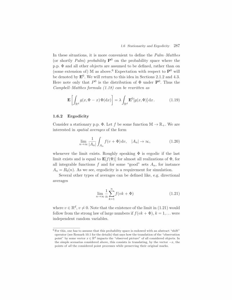
In these situations, it is more convenient to define the Palm–Matthes(or shortly Palm) probability P0 on the probability space where thep.p. Φ and all other objects are assumed to be defined, rather than on(some extension of) M as above.6 Expectation with respect to P0 willbe denoted by E0. We will return to this idea in Sections 2.1.2 and 4.3.Here note only that P 0 is the distribution of Φ under P0. Thus theCampbell–Matthes formula (1.18) can be rewritten as
E[∫
Rd
g(x,Φ − x)Φ(dx)]
= λ
∫Rd
E0[g(x,Φ)]dx. (1.19)
1.6.2 Ergodicity
Consider a stationary p.p. Φ. Let f be some function M → R+. We areinterested in spatial averages of the form
limn→∞
1|An|
∫An
f(v + Φ)dv, |An| → ∞, (1.20)
whenever the limit exists. Roughly speaking Φ is ergodic if the lastlimit exists and is equal to E[f(Φ)] for almost all realizations of Φ, forall integrable functions f and for some “good” sets An, for instanceAn = B0(n). As we see, ergodicity is a requirement for simulation.
Several other types of averages can be defined like, e.g. directionalaverages
limn→∞
1n
n∑k=1
f(vk + Φ) (1.21)
where v ∈ Rd, v = 0. Note that the existence of the limit in (1.21) would
follow from the strong law of large numbers if f(vk + Φ), k = 1, . . . wereindependent random variables.
6 For this, one has to assume that this probability space is endowed with an abstract “shift”operator (see Remark 10.1 for the details) that says how the translation of the “observationpoint” by some vector x ∈ R
d impacts the “observed picture” of all considered objects. Inthe simple scenarios considered above, this consists in translating, by the vector −x, thepoints of all the considered point processes while preserving their original marks.
288 Poisson Point Process
Definition 1.12. We say that a stationary p.p. Φ
• is mixing if
Pv + Φ ∈ Γ,Φ ∈ ∆→PΦ ∈ ΓPΦ ∈ ∆ when |v| → ∞,
for all for configuration sets Γ and ∆ that depend on therealization of the p.p. in some bounded set;
• is ergodic if
limt→∞
1(2t)d
∫[−t,t]d
(v + Φ∈Γ,Φ∈∆
)dv = PΦ∈ΓPΦ∈∆,
for all such Γ,∆.
By the dominated convergence theorem, we have the following fact:
Corollary 1.20. A mixing point process is ergodic.
Also
Proposition 1.21. A homogeneous Poisson p.p. Φ is mixing and henceergodic.
Proof. For Γ and ∆ as in Definition 1.12, Γ − v = −v + φ:φ ∈ Γ and∆ depend on the configuration of points in disjoint subsets of R
d. Thus,by the very definition of the Poisson p.p., (v + Φ ∈ Γ) = (Φ ∈ Γ − v)and (Φ ∈ ∆) are independent.
Coming back to our ergodic postulates, call a sequence Aiof convex sets a convex averaging sequence if A1 ⊂ A2 ⊂ ·· · ⊂ R
d
and supr:An contains a ball of radius r → ∞ when n → ∞. One cancan prove the following result for general stationary point processes(cf. Daley and Ver-Jones, [9], Section 10.3; Pugh and Shub, [37]).
Proposition 1.22. Suppose that Φ is translation invariant. Then thefollowing statements are equivalent.

1.6 Stationarity and Ergodicity 289
(1) Φ is ergodic.(2) For any f such that E[f(Φ)] < ∞ and for all vectors v ∈
Rd, possibly off some countable set of hyperplanes in R
d (ahyperplane is not assumed to contain the origin), the limit(1.21) almost surely exists.
(3) For any f such that E[f(Φ)] < ∞ and any convex averagingsequence Ai the limit in (1.20) is equal to E[f(Φ)] almostsurely.
(4) Any function f of Φ that is translation invariant (i.e. suchthat for all v ∈ R
d, f(v + Φ) = f(Φ) almost surely), is almostsurely constant.
In many problems, rather than (1.20), one is interested in anotherkind of spatial average that will be referred to as spatial point averagesin what follows, and which are of the form
limn→∞
1Φ(An)
∑xi∈An
f(Φ − xi), |An| → ∞, (1.22)
whenever the limit exists. The following result can be found in, e.g.,Daley and Vere-Jones ([9], cf. Proposition 12.2.VI).
Proposition 1.23. If Φ is translation invariant and ergodic, for all f
and for any convex averaging sequence An
limt→∞
1Φ(An)
∑xi∈An
f(Φ − xi) =∫
f(φ)P 0(dφ) = E0[f(Φ)] a.s.,
(1.23)provided E0[f(Φ)] < ∞.
The above ergodic property says that the distribution P 0 of the pointprocess “seen from its typical point” (cf. Remark 1.1) is also the dis-tribution of Φ “seen from its randomly chosen point”.
In Part V in Volume II we will also consider route averages asso-ciated with certain multihop routing algorithms. A routing algorithmis defined through a map AD:Rd × M → R
d, where AD(X,Φ) ∈ Φ, for
290 Poisson Point Process
X ∈ Φ, is the next hop from X on the route. This next hop dependson the destination node D and also on the rest of the point process Φ.
Within this setting, when denoting by AnD the nth order iterate of
AD and by N(O,D) the number of hops from origin O to destination D,route averages are quantities of the type
1N(O,D)
N(O,D)∑n=1
f(AnD(O,Φ) − An−1
D (O,Φ)),
where f is some function Rd → R
+. One of the key questions withinthis context is the existence of a limit for the last empirical averagewhen |O − D| → ∞.

2Marked Point Processes and Shot-Noise Fields
In a marked point process (m.p.p.), a mark belonging to some measur-able space and carrying some information is attached to each point.
2.1 Marked Point Processes
Consider a d-dimensional Euclidean space Rd, d ≥ 1, as the state space
of the point process. Consider a second space R, ≥ 1, called the space
of marks. A marked p.p. Φ (with points in Rd and marks in R
) is alocally finite, random set of points in R
d, with some random vector inR
attached to each point.One can represent a marked point process either as a collection of
pairs Φ = (xi,mi)i, where Φ = xi is the set of points and mi theset of marks, or as a point measure
Φ =∑
i
ε(xi,mi), (2.1)
where ε(x,m) is the Dirac measure on the Cartesian product Rd × R
with an atom at (x,m). Both representations suggest that Φ is a p.p. inthe space R
d × R, which is a correct and often useful observation. We
denote the space of its realizations (locally finite counting measures on
291

292 Marked Point Processes and Shot-Noise Fields
Rd × R
) by M. As a point process in this extended space, Φ has oneimportant particularity inherited from its construction, namely thatΦ(A × R
) is finite for any bounded set A ⊂ Rd, which is not true for
a general p.p. in this space.
2.1.1 Independent Marking
An important special case of marked p.p. is the independentlymarked p.p.
Definition 2.1. A marked p.p. is said to be independently marked(i.m.) if, given the locations of the points Φ = xi, the marks are mutu-ally independent random vectors in R
, and if the conditional distribu-tion of the mark m of a point x ∈ Φ depends only on the location of thispoint x it is attached to; i.e., Pm ∈ · | Φ = Pm ∈ · | x = Fx(dm)for some probability kernel or marks F·(·) from R
d to R.
An i.m.p.p. can also be seen as a random transformation of pointsby a particular probability transition kernel (cf. Section 1.3.3). Thisleads to immediate results in the Poisson case.
Corollary 2.1. An independently marked Poisson p.p. Φ with inten-sity measure Λ on R
d and marks with distributions Fx(dm) on R is a
Poisson p.p. on Rd × R
with intensity measure
Λ(A × K) =∫
Ap(x,K)Λ(dx), A ⊂ R
d,K ⊂ R,
where p(x,K) =∫K Fx(dm). Consequently, its Laplace transform is
equal to
LΦ(f) = E[exp
−∑
i
f(xi,mi)]
= exp
−∫
Rd
(1 −
∫R
e−f(x,m) Fx(dm))
Λ(dx)
, (2.2)
for all functions f :Rd+l → R+.
2.1 Marked Point Processes 293
Proof. Take d′ = d + , and consider the following transition kernelfrom R
d to Rd′
:
p(x,A × K) = (x ∈ A)p(x,K) x ∈ Rd,A ⊂ R
d,K ⊂ R. (2.3)
The independently marked Poisson p.p. can be seen as a transformationof the (non-marked) Poisson p.p. of intensity Λ on R
d by the probabilitykernel (2.3). The result follows from the Displacement Theorem (seeTheorem 1.10).
Remark. An immediate consequence of the above result and ofSlivnyak’s theorem is that the reduced Palm distribution P !
(x,m)(·) of
i.m. Poisson p.p. Φ given a point at x with mark m is that of thei.m. Poisson p.p. with intensity measure Λ and with mark distributionFx(dm). Moreover, a mere rewriting of the reduced Campbell formulafor Poisson point processes yields
E[∫
Rd×R
f(x,m,Φ \ x)Φ(d(x,m))]
=∫
Rd
∫R
E[f(x,m, Φ)
]Fx(dm)M(dx). (2.4)
In the general case, independent marking leads to the followingresults:
Corollary 2.2. Let Φ be an i.m.p.p.
(1) The mean measure of Φ is equal to
E[Φ(A × K)] =∫
AFx(K)M(dx) A ⊂ R
d, K ⊂ R,
(2.5)where M(A) = E[Φ(A)] is the mean measure of the points Φof Φ.
(2) The reduced Palm distribution P !(x,m)(·) of Φ given a point
at x with mark m is equal to the distribution of the i.m.p.p.,with points distributed according to the reduced Palm distri-bution P !
x of Φ and with the same mark distributions Fx(dm).

294 Marked Point Processes and Shot-Noise Fields
(3) (Reduced Campbell’s formula for i.m.p.p.) For all non-negative functions f defined on R
d × R × M,
E[∫
Rd×R
f(x,m, Φ \ ε(x,m))Φ(d(x,m))]
=∫
Rd
∫R
∫M
f(x,m,φ)P !(x,m)(dφ)Fx(dm)M(dx). (2.6)
Proof. We only prove the first statement; for the remaining ones seee.g., Daley and Vere-Jones ([9]). Conditioning on Φ, we have
E[Φ(A,K)] = E[∫
Rd
∫R
(x ∈ A) (m ∈ K)Φ(d(x,m))]
= E[∫
Rd
(x ∈ A)Fx(K)Φ(dx)]
=∫
AFx(K)M(dx),
which proves (2.5).
2.1.2 Typical Mark of a Stationary Point Process
Many stochastic models constructed out of independently marked pointprocesses may also be seen as marked point processes, however, they areoften no longer independently marked. The Matern model consideredbelow in Section 2.1.3 is an example of such a situation; the Voronoitessellation of Chapter 4 is another.
Consider thus a general marked p.p. Φ as in (2.1). In general, it isnot true that, given the locations of points of Φ, the mark m of somex ∈ Φ is independent of other marks with its distribution determinedonly by x. However, it is still interesting and even of primary interestto the analysis of Φ to know the conditional distribution Pm ∈ · | xof mark m given its point is located at x. In what follows, we treat thisquestion in the case of a stationary p.p.
Definition 2.2. A marked point process (2.1) is said to be station-ary if for any v ∈ R
d, the distributions of v + Φ =∑
i ε(v+xi,mi) and Φare the same. The constant λ = E[Φ(B)] = E[Φ(B × R
)], where B hasLebesgue measure 1, is called its intensity.

2.1 Marked Point Processes 295
Note that in the above formulation the translation by the vector v
“acts” on the points of Φ and not on their marks, thus ensuring thatshifted points “preserve their marks”.
Define the Campbell–Matthes measure C of the marked p.p. Φ as
C(B × K) = E[∫
Rd
∫R
(x ∈ B) (m ∈ K)Φ(d(x,m))]. (2.7)
If λ < ∞, by arguments similar to those used in Section 1.4, one canshow that it admits the representation
C(B × K) = λ|B|ν(K). (2.8)
Definition 2.3.(Palm distribution of the marks) The probabilitymeasure ν(·) on the space of marks R
given in (2.8) is called the Palmdistribution of the marks.
The Palm distribution ν of the marks may be interpreted as theconditional distribution ν(·) = Pm ∈ · | 0 ∈ Φ of the mark m of apoint located at the origin 0, given 0 ∈ Φ. Not surprisingly, takingf(x,m,φ) = (x ∈ B) (m ∈ K) in (2.6) and comparing to (2.8) we findthat
Corollary 2.3. Consider a stationary i.m.p.p. For (almost all) x, theprobability kernel of marks Fx(·) = ν(· · ·) is constant and equal to thePalm distribution of the marks.
In view of the above observation, we shall sometimes say thatthe points of a stationary i.m.p.p. are independently and identicallymarked.
Under the Palm probability P0 of a stationary p.p. Φ, all the objectsdefined on the same space as Φ have their distributions “seen” from thetypical point of the process, which is located at 0 (cf. the discussionat the end of Section 1.6.1). In the case of a stationary m.p.p., underP0, the mark attached to the point at 0 has the distribution ν; thisexplains why it is also called the distribution of the typical mark. In
296 Marked Point Processes and Shot-Noise Fields
this context, the Campbell–Matthes formula (1.18) can be rewritten toencompass the marks
E[∫
Rd
g(x, Φ − x)Φ(dx)]
= λ
∫Rd
E0[g(x, Φ)]dx. (2.9)
Note that in the above formula, in contrast to (2.6), the m.p.p. Φ isnot treated as some p.p. in a higher dimension but rather as a pointprocess Φ on a probability space on which marks are defined as well.This approach is more convenient in the case of a stationary m.p.p.,since it exploits the property of the invariance of the distribution of Φwith respect to a specific translation of points which preserves marks(cf. Definition 2.2).1
The following observation is a consequence of Slivnyak’s theo-rem 1.13:
Remark 2.1. Consider a stationary i.m. Poisson p.p. Φ with a proba-bility kernel of marks Fx such that Fx(·) = F (·). One can conclude fromCorollary 2.3 and the Remark after Corollary 2.1 that its distributionunder the Palm probability P0 is equal to that of Φ + ε(0,m0), whereΦ is taken under the original (stationary distribution) P and the markm0 of the point at the origin is independent of Φ and has the samedistribution F (·) as for any of the points of Φ.
Almost all stochastic models considered throughout this monographare constructed from some marked point processes. Here is a first exam-ple driven by an i.m. Poisson p.p.
2.1.3 Matern Hard Core Model
Hard core models form a generic class of point processes whose pointsare never closer to each other than some given distance, say h > 0 (asif the points were the centers of some hard balls of radius 1
2h). For the
1 The Palm probability P0 can be defined as the Palm distribution of the marks in thecase when the whole configuration of points and all other random objects existing onthe probability space “seen” from a given point of x ∈ Φ is considered as a mark of thispoint — the so called universal mark. This requires a more abstract space of marks thanR
considered above; see Section 10.2 for more details.
2.1 Marked Point Processes 297
Poisson p.p. there exists no h > 0 such that the p.p. satisfies the hardcore property for h.
We now present a hard core p.p. constructed from an underlyingPoisson p.p. by removing certain points of the Poisson p.p. depend-ing on the positions of the neighboring points and additional marksattached to the points.
Let Φ be a Poisson p.p. of intensity λ on Rd:
Φ =∑
i
εxi .
Let us consider the following independently marked version of thisprocess:
Φ =∑
i
ε(xi,Ui),
where Uii are random variables uniformly distributed on [0,1]. Definenew marks mi of points of Φ by
mi = (Ui < Uj for all yj ∈ Bxi(h)\xi). (2.10)
Interpreting Ui as the “age” of point xi, one can say that mi is theindicator that the point xi is the “youngest” one among all the pointsin its neighborhood Bxi(h).
The Matern hard core (MHC) point process is defined by:
ΦMHC =∑
i
miεxi . (2.11)
ΦMHC is thus an example of a dependent thinning of Φ. In contrast towhat happens for an independent thinning of a Poisson p.p. as con-sidered in Section 1.3.2, the resulting MHC p.p. is not a Poisson p.p.Nevertheless some characteristics of the MHC p.p. can be evaluatedexplicitly, as we show shortly. Consider also the “whole” marked p.p.
ΦMHC =∑
i
ε(xi,(Ui,mi)). (2.12)
Clearly ΦMHC is not independently marked, because of mi. Never-theless ΦMHC (as well as ΦMHC) is stationary. This follows from the

298 Marked Point Processes and Shot-Noise Fields
following fact. Let ΦMHC(Φ) denote the (deterministic) mapping fromΦ to ΦMHC. Then for all v ∈ R
d,
ΦMHC(v + Φ) = v + ΦMHC(Φ)
with v + Φ interpreted as in Definition 2.2.We now identify the distribution of marks by first finding the distri-
bution of the typical mark of ΦMHC and then calculating the intensityλMHC of the p.p. ΦMHC. For B ⊂ R
d and 0 ≤ a ≤ 1, by Slivnyak’s the-orem (see Proposition 1.13)
C(B × ([0,a] × 1))
= E
[∫B
∫[0,a]
(u < Uj for allyj ∈ Bx(h) ∩ Φ \ x)Φ(d(x,u))
]
= λ|B|∫
B
∫ a
0P
∑
(xj ,Uj)∈Φ
(Uj ≤ u)εxj
(Bx(h)) = 0
du dx
= λ|B|∫ a
0e−λuνdhd
du = |B|1 − e−λaνdhd
νdhd,
where νd =√
πd/Γ(1 + d/2) is the volume of the ball B0(1) of Rd. Com-
paring the last formula with (2.8), we find that
ν(du × 1) = P0U0 ∈ du,m0 = 1 = e−λuνdhddu,
for 0 ≤ u ≤ 1, where (U0,m0) is the mark of the point located at 0under P0. In this formula, we recognize that U0 has the original uniformdistribution of marks Ui and, given U0 = u, the point at 0 is retainedin ΦMHC (i.e. m0 = 1) with probability e−λuνdhd
.In order to calculate the intensity λMHC of the Matern p.p., we take
a set B with volume |B| = 1 and obtain
λMHC = C(B × [0,1] × 1) = λP0m0 = 1 =1 − e−λνdhd
νdhd.
Notice that when λ → ∞, λMHC 1νdhd . Hence the MHC process packs
hard spheres of radius h/2 with a volume fraction (proportion of spacecovered by spheres — see Section 3.4 for a general definition) of
p =1
νdhdνd
(h
2
)d
=12d
. (2.13)
2.1 Marked Point Processes 299
Remark 2.2. The value 1/2d is a good lower bound (sometimes calledthe “greedy” one) for the volume fraction obtained by any saturatedhard sphere packing. A configuration of non-overlapping (hard) ballswith the same radius is called saturated if no further ball with thisradius can be added without violating the no-overlap constraint. Let p
be the fraction of the space (say, in some empirical mean sense) cov-ered by a saturated configuration Bxi(R)i of balls with radius R.The saturation condition implies that all points of the space are atdistance no larger than 2R from the center of some ball of this config-uration (otherwise a new ball could be added there). This implies thatwhen doubling the radius of each ball of the original configuration,one obtains a full coverage of the space, i.e., Ξ =
⋃i Bxi(2R) = R
d. Thevolume fraction p′ of Ξ is thus equal to 1. On the other hand, whendenoting by p the volume fraction of the original configuration, we getthat p′ ≤ 2dp (when using the multiplication of the radius by 2 and theinequality stemming from the overlapping). Thus 1 = p′ ≤ 2dp, whichimplies p ≥ 1/2d.
For comparison, an upper bound given in ([6]) for the volumefraction of any hard sphere model valid for all d ≥ 1 is (d/2 + 1)2−d/2
and the best currently known upper bound is 2−0.5990d(1+o(1)) whend → ∞ ([26]).
Table 2.1 gives the volume fractions of some classical hard-spheremodels for d = 1,2,3.
Example 2.1 (Carrier sense multiple access). The above MHCmodel can be used as a (very) simple model of the instantaneous repar-tition of active nodes in an ad hoc network using carrier sensing mutipleaccess (CSMA) protocol (see Section 25.1.3 in Volume II). In this pro-tocol, a node which wants to access the shared wireless medium sensesits occupation and refrains from transmitting if the channel is alreadylocally occupied. Hence, each active node creates some exclusion regionaround itself preventing other nodes located in this region from trans-mitting. The simplest possible model taking such an exclusion is theMHC with a radius h equal to the sensing (exclusion) range of CSMA.

300 Marked Point Processes and Shot-Noise Fields
Table 2.1. Volume fractions of some classical hard-sphere models.
Modeldimension saturated Matern RSA Densest packing
1 0.5 0.747598... 1.2 0.25 0.54700 0.90689...3 0.125 0.38278 0.74048...
Volume fractions of some classical hard-sphere models. The left col-umn gives the exact value (2.13) for the saturated Matern model.The center column gives the value of the saturated RSA (RandomSequential Addition) model. For d = 1 this model, known as theRenyi car parking problem, has an exact solution; for d = 2,3 weused simulated values taken from [44]. It should be mentioned thatthe construction of the RSA model on the whole space is not trivial;see [43, 36] for a rigorous proof of the convergence of the empiricalvolume fractions when the observation window tends to infinity. Thedensest packing is given on the rightmost column. On the plane thedensest packing is that of the hexagonal lattice (cf. Section 19.3.2in Volume II), the volume fraction of which is 1/6π
√3. For d = 3
it was conjectured by Kepler in 1611 and proved only recently thatthe cubic or hexagonal packings (which both have volume fractionπ/(3
√2)) are the densest possible.
Note that in this model λMHC = λMHC(λ,h) corresponds to the spatialdensity of active nodes in the ad hoc network of density λ, when thisnetwork uses CSMA with a sensing range of h.
2.2 Shot-Noise
2.2.1 General Point Processes
A shot-noise (SN) field is a non-negative vector random field IΦ(y)defined for all y in some Euclidean space and which is a functional ofa marked point process Φ. Here is a list of the spaces involved in itsdefinition:
• The field is defined on Rd′
i.e., for all y ∈ Rd′
;• The vector field takes its values in (R+)k, i.e., IΦ(y) ∈ R
+k
for all y;• It is generated by a marked point process Φ =
∑i ε(xi,mi) on
Rd with marks in R
.
The additional ingredient for its definition is some non-negativeresponse function L = (L1, . . . ,Lk):Rd′ × R
d × R → (R+)k.

2.2 Shot-Noise 301
Definition 2.4. Under the setting described above, the SN field asso-ciated with the marked point process Φ and the response function L isdefined by
IΦ(y) = (I1(y), . . . , Ik(y))
=∫
Rd
∫R
L(y,x,m)Φ(d(x,m))
=∑
(xi,mi)∈Φ
L(y,xi,mi), y ∈ Rd′
,
where the integral and the sum are evaluated component-wise for thevector response function L.
Remark. The case where the field lives in the same space as thepoint process Φ (i.e., d′ = d) is the most common. The term “Shot-Noise” comes from this special case with d = 1. It describes a stochasticprocess with ‘shots’ taking place at the epochs Xi of a Poisson pointprocess on the real line, which represents time. The shot at Xi has aneffect over time of the form l(t − Xi), where l:R → R
+ is a functionwhich is usually such that l(x) = 0 for x < 0 (non anticipativeness) anddecreasing for x ≥ 0. The Shot-Noise at time t,
I(t) =∑
i
l(t − Xi) ,
is then the ‘sum’ of the effects of the shots that took place before time t.Since L is positive, IΦ(y) is well defined but can be infinite. In the
sequel, we require this random field to be a.s. finite and moreover tohave finite expectation. Using the Campbell formula (2.6) we can easilyexpress this expectation in the case of an i.m.p.p. Φ.
Proposition 2.4. Let IΦ(y) be the SN field as above and assume thatΦ is an i.m.p.p. Then
E[IΦ(y)] =∫
Rd×R
L(y,x,m)F (dm | x)M(dx) (2.14)
componentwise.

302 Marked Point Processes and Shot-Noise Fields
Proof. We have by (2.6)
E[IΦ(y)] = E[∫
Rd
∫R
L(y,x,m)Φ(d(x,m))]
=∫
Rd×R
L(y,x,m)F (dm | x)M(dx).
Assuming that the right-hand side in (2.14) is finite for all y, weguarantee that each random vector IΦ(y) has finite expectation andthus is finite almost surely. This however is not sufficient to be able tosay that with probability 1 the whole field IΦ(y):y ∈ R
d′ is finite. Forthis latter, as well as for a continuity property of the paths of this field(which will be useful later on) we prove the following technical result.
Proposition 2.5. Let IΦ(y) be the shot-noise field defined above andassume that Φ is an i.m.p.p. If for each y ∈ R
d′, there exists εy > 0 such
that ∫Rd
∫R
supz∈By(εy)
L(z,x,m)F (dm | x)M(dx) < ∞ (2.15)
componentwise, then with probability 1, the field IΦ(y) is finite for ally ∈ R
d′. If moreover the response function L(y,x,m) is a continuous
(lower semi-continuous) function in y for any fixed (x,m), then withprobability 1, the field IΦ(y) has continuous (lower semi-continuous)paths.
Proof. From the open covering By(εy):y ∈ Rd′ of R
d′one can choose
a countable covering Byw(εyw):w = 1,2, . . . (this is possible since Rd′
is separable). From (2.15), there exists a subset Ω′ of the space on whichΦ is defined and having probability one, such that for all ω ∈ Ω′
I ′(yw) =∫
Rd
∫R
supz∈Byw (εyw )
L(z,x,m)Φ(d(x,m)) < ∞,
for all w = 1,2, . . .. Consequently, for all ω ∈ Ω′ and z ∈ Rd′
, IΦ(z) ≤I ′(yw(z)) < ∞ componentwise, where w(z) denotes the center of theball of radius εyw(z) of the countable coverage which covers z; i.e.,z ∈ Byw(z)(εyw(z)). This proves the first statement.

2.2 Shot-Noise 303
For continuity (lower semi-continuity), take any z ∈ Rd′
and zn → z
(zn z). For sufficiently large n, zn and z belong to Byw(z)(εyw(z)).Then by dominated convergence,
limn→∞IΦ(zn) =
∫Rd
∫R
limn→∞L(zn,x,m)Φ(d(x,m)) = IΦ(z) ,
because L is continuous (lower semi-continuous) in its firstargument.
2.2.2 Poisson Point Processes
In the case of a SN I(y) = IΦ(y) generated by an i.m. Poisson p.p. Φ, thedistribution of the SN vector I(y) is known in terms of its multivariateLaplace transform LI(y)(t1, . . . , tk) = E[e−∑k
i=1 tiIi(y)].
Proposition 2.6. Suppose that Φ is an i.m. Poisson p.p. with intensitymeasure Λ and mark distribution Fx(dm). Consider the SN I(y) =IΦ(y) with response function L = (L1, . . . ,Lk). Then
LI(y)(t1, . . . , tk)= exp−∫
Rd
∫R
(1−e−∑k
i=1 tiLi(y,x,m))
Fx(dm)Λ(dx)
.
(2.16)
Proof. Observe that LI(y)(t1, . . . , tk)=LΦ(f) where LΦ(·) is the Laplacetransform of Φ at the function f =f(x,m)= −∑k
i=1 tiLi(y,x,m).Equation (2.16) follows from Corollary 2.1 and Proposition 1.5.
One can evaluate explicitly the higher moments of I by differenti-ating the above formula at 0.
Joint Distribution of the Field at Several Points. Let I(y) =IΦ(y) be an SN field with response function L as in Definition 2.4 andlet Ψ be a linear transformation (R+)k×n → (R+)k′
for some integers n
and k′. Then
I ′Φ(y1, . . . ,yn) = Ψ(I(y1), . . . , I(yn))
304 Marked Point Processes and Shot-Noise Fields
is an SN field on Rd′×n with response function
L′((y1, . . . ,yn),x,m) = Ψ(L(y1,x,m), . . . ,L(yn,x,m)).
In particular, taking Ψ(a1, . . . ,an) =∑n
j=1 aj , we see that the n-dimensional aggregate I
∑
Φ(y1, . . . ,yn) =
∑nj=1 I(yj) is a SN on R
d′×n
with associated function L∑
((y1, . . . ,yn),x,m) =∑n
j=1 L(yj ,x,m). Sim-ilarly, the integrals I
∫
Φ(A) =
∫A I(y)dy can be interpreted as a shot-
noise field on the space of (say) closed subsets A ⊂ Rd′
. As anotherimmediate consequence of the above formulation, we have the nextresult by setting k′ = k × n, using the identity transformation Ψ andappealing to Proposition 2.6:
Corollary 2.7. Let I = IΦ(y) be as in Proposition 2.6. Then the jointLaplace transform, LI(y)(t) of the vector I(y) = (I(y1), . . . , I(yn)) isgiven by
LI(y)(t)= exp−∫
Rd
∫R
(1−e−∑n
j=1∑k
i=1 tijLi(yj ,x,m))Fx(dm)Λ(dx)
,
where t = (tij :j = 1, . . . ,n, i = 1, . . . ,k).
Absolute Continuity. In the following proposition, we give simpleconditions for the Poisson SN vector IΦ(y) to have a probability lawwhich is absolutely continuous (has a density) with respect to Lebesguemeasure. This property can be used to derive the distribution func-tion of the shot-noise from its Laplace (or Fourier) transform via thePlancherel–Parseval Theorem (cf. Section 12.1).
Proposition 2.8. Let I = IΦ(y) be as in Proposition 2.6.If Λ(Rd) = ∞ and if, for each A ⊂ (R+)k of Lebesgue measure 0,∫
Rd
∫R
(L(y,x,m) ∈ A)Fx(dm)Λ(dx) = 0 , (2.17)
then, for all y ∈ Rd′
, the random vector IΦ(y) is absolutely continuouswith respect to the k-dimensional Lebesgue measure (i.e. has a density).

2.3 Interference Field as Shot-Noise 305
Proof. Fix y ∈ Rd′
; without loss of generality let y = 0. Take A ⊂ (R+)k
of k-dimensional Lebesgue measure 0. For any r > 0
PIΦ(0) ∈ A = PIr + Icr ∈ A,
where Ir =∫|x|≤r
∫R L(0,x,m)Φ(d(x,m)) and Ic
r =∫|x|>r
∫R L(0,x,m)
Φ(d(x,m)). By the Poisson assumption Ir and Icr are independent.
Moreover
PIΦ(0) ∈ A =∞∑
n=0
P
Ir + Icr ∈ A | Φ
x : |x| ≤ r
= n
×P
Φx : |x| ≤ r
= n.
Recall from the discussion at the end of Section 1.1.1 that conditionedon Φ
x: |x| ≤ r
= n, with n > 0, the random variable Ir can be rep-
resented as the sum of n independent random variables, distributed asL(0,x,m) where x and m have joint distribution
1Λ(x: |x| ≤ r)Fx(dm)Λ(dx).
Thus, by (2.17)
P
Ir + Icr ∈ A|Φx: |x| ≤ r = n
= 0.
Consequently,
PIΦ(0) ∈ A ≤ PΦx: |x| ≤ r = 0
→ 0 when r → ∞because Λ(Rd) = ∞. This completes the proof.
2.3 Interference Field as Shot-Noise
Consider a collection of transmitters distributed in the space andsharing a common radio medium. Following the observations made inChapter 23 in Volume II, assume that signal attenuation depends ondistance (cf. Section 23.1 in Volume II) and some stochastic ingredients(cf. Section 23.2 in Volume II).
The total power received from this collection of transmitters ata given location is in essence a shot-noise field at this location. Forinstance in the case of a planar model with omni-directional antennas,

306 Marked Point Processes and Shot-Noise Fields
the simplest model consists of
• a collection of points xi representing the locations of trans-mitters on the plane R
2 (d = 2 in Definition 2.4);• marks mi = pi representing the powers of the transmitters
( = 1); and• a scalar (k = 1) response function L(y,x,p) = p/l(|x − y|),
where l is the omni-directional path-loss function (cf. Sec-tion 23.1.2 in Volume II).
As we shall see, fine elements of the radio wave propagation model(antenna azimuth, random fading model, etc.) can be taken intoaccount by enriching the marks of the p.p.
As outlined in Section 24.3.4 in Volume II, the total power receivedfrom a set of transmitters scattered in the plane can often be consideredas interference or noise with respect to the signal received from one (ormore) transmitter(s) not belonging to this set. Within this setting,this total power plays a key role in detection theory as explained inSection 24.3.4 in Volume II. The fact that the interference field of sucha set of transmitters can be interpreted as a shot-noise field opensnew ways of assessing its statistical properties. In the same way asRayleigh fading was shown to be an efficient statistical model bettersuited to assessing the fluctuations of a multipath channel than solvingthe electromagnetic field equations, the shot-noise model can be seento be an efficient statistical model for predicting the fluctuations of theinterference field. This is often more practical than evaluating exactlythe power of interference.
2.3.1 Standard Stochastic Scenario
Consider a marked point process Φ = xi,pi with points on the planexi ∈ R
2 and marks pi ∈ R+. Points represent transmitter locations
and marks emitted powers. Consider some isotropic or ommi-directionalpath-loss (OPL) function l, for example, models OPL 1–OPL 3described in detail in Example 23.3 in Volume II and defined as follows:
(OPL 1) l(r) = (Amax(r0, r))β,(OPL 2) l(r) = (1 + Ar)β,(OPL 3) l(r) = (Ar)β,
2.3 Interference Field as Shot-Noise 307
for some A > 0, r0 > 0 and β > 2, where β is called the path-loss expo-nent. Assuming the signals are transmitted and received by omni-directional antennas, the total power received at some location y is
I(y) = IΦ(y) =∑
(xi,pi)∈Φ
pi
l(|y − xi|) , y ∈ R2. (2.18)
We shall often consider the following standard stochastic scenariofor the above interference shot-noise field:
(1) Φ is a stationary i.m.p.p. with points in R2 and intensity λ;
(2) the marks have some distribution Pp ≤ s = G(s) that doesnot depend on the location of the point.
Notice that this model excludes power control as described in Sec-tion 25.2 in Volume II where powers are functions of the transmitterlocations.
Kendall-like Notation for the Standard Interference Model.Mimicking Kendall’s notation in queuing theory, we call the above stan-dard stochastic scenario of SN a GI/GI interference model, where thefirst GI denotes a general independently marked stationary p.p. andthe second GI stands for a general mark distribution. Some specialcases are:
M/· if the underlying i.m.p.p. Φ is Poisson;D/· if the underlying i.m.p.p. Φ is deterministic;·/M if the marks are exponentially distributed; i.e. G(s) = 1 −e−µs with µ ≥ 0.·/D if the marks are deterministic (constant).
For instance, the interference field in a MANET with nodes locatedaccording to a Poisson p.p. and without power control (see Sec-tion 25.3.1 in Volume II) can be seen as an M/· SN. Similarly, thefamous honeycomb model used in certain cellular network models forrepresenting the location of base stations leads to a downlink interfer-ence field which falls in the D/· SN class provided no power control isused (see Section 25.3.2 in Volume II).
Remark 2.3. Assume that emitted powers pi = p are constant andthat we have some Rayleigh fading (see Section 23.2.4 in Volume II).
308 Marked Point Processes and Shot-Noise Fields
Then the power received at the location y from a transmitter at xi
is equal to pFi/l(|xi − y|), where Fi is an exponential random vari-able with mean 1. Thus, interpreting pFi as a “virtual power” (whichis hence exponential with mean p), the GI/M model may be used todescribe the interference in the presence of Rayleigh fading. In whatfollows, we shall most often work directly with the virtual power, orequivalently assume that Rayleigh fading is represented by an expo-nential random variable of parameter µ = p−1.
The independence between Fi for different transmitters, which isassumed in the GI/M model, can be justified if the point process issparse on the scale of the coherence distance (see Section 23.3 in Vol-ume II). However this SN representation is valid only for one givenlocation. Indeed, using the same value of the fading Fi from point xi todifferent locations y ∈ R
2 would not be a reasonable assumption as thechannel conditions change significantly when y varies more than thecoherence distance. We will return to this problem in Section 2.3.3.
Corollary 2.9. The mean total received power in the GI/GI model isconstant and equal to
E[I(y)] = E[I]
= E[p]λ∫
R2
1l(|y|) dy
=∫ ∞
0(1 − G(s))ds 2πλ
∫ ∞
0
r
l(r)dr . (2.19)
The Laplace transform of the received power in the M/GI model isequal to
LI(y)(t) = LI(t) = exp
−2πλ
∫ ∞
0r(1 − Lp
(t/l(r)
))dr
, (2.20)
where Lp(t) =∫∞
0 e−ts G(ds) is the Laplace transform of the transmit-ted power. The second moment in the M/GI model is equal to
E[I2(y)] = (E[I])2 + E[p2]2πλ
∫ ∞
0
r
(l(r))2 dr . (2.21)
2.3 Interference Field as Shot-Noise 309
Example 2.2. For the M/M model, these values are equal to
E[I] =2πλ
µ
∫ ∞
0
r
l(r)dr , (2.22)
LI(t) = exp
−2πλ
∫ ∞
0
r
1 + µl(r)/tdr
. (2.23)
Below, we use the fact that∫ ∞
0
11 + xu
dx = 1/uΓ(1/u)Γ(1 − 1/u). (2.24)
Assuming OPL 3 for l, one obtains
LI(t) = exp
−λ
(t
µ
)2/β K(β)A2
, (2.25)
with
K(β) =2π2
β sin(2π/β)=
2πΓ(2/β)Γ(1 − 2/β)β
. (2.26)
Assuming OPL 1 for l with β = 4, one obtains
LI(t) = exp[λπ
A2
√t
µarctan
((Ar0)2
õ
t
)− λπ2
2A2
√t
µ− λπr2
0t
t + (Ar0)4µ
]. (2.27)
Corollary 2.10. Consider an M/GI model with the non-null marks(i.e., G(0) < 1), for which at least one of the following conditions issatisfied: the distribution function G of the mark admits a density orthe OPL function l(r) is strictly decreasing. Then for 0 ≤ a ≤ b
Pa ≤ I ≤ b =∫ ∞
−∞LI(2iπs)
e−2iπbs − e−2iπas
2iπsds, (2.28)
provided∫∞−∞ |LI(2iπs)|2 ds < ∞.

310 Marked Point Processes and Shot-Noise Fields
Proof. Under our assumptions, by Proposition 2.8, the SN I has adensity that is square integrable provided the Fourier transform of I
is square integrable (see [14, p.510]). Then the result follows by thePlancherel–Parseval theorem (see Lemma 12.1).
Remark 2.4. For the GI/GI scenario with OPL 1 and OPL 2 andE[p] =
∫∞0 sG(ds) < ∞ we can conclude from Proposition 2.5 and for-
mula (2.19) with l(r) replaced by l(max(r − ε,0)) that, with probability1, the SN field IΦ(y) is finite for all y ∈ R
2. For OPL 3 one has to bemore careful. Note that by (2.19) the integral expressing E[I] is infinitein this case for β > 2 due the pole at the origin (cf. also Example 23.3in Volume II). Consequently, the simplified isotropic path-loss functionOPL 3 cannot be used to model the mean interference field created by ahomogeneous i.m.p.p. on the plane. However, with probability 1, IΦ(y)is finite for all y ∈ R
2 except for y ∈ Φ. One can prove this by consid-ering the mean of the shot-noise created by transmitters outside somevicinity of the receiver (which is finite) and knowing that the numberof transmitters within this vicinity is finite with probability 1.
Using the explicit formula (2.20) one can also check that in theM/GI model with OPL 3 and G(0) < 1 the Fourier transform LI(2iπ)of I is square integrable.
Note that for the M/GI model, Proposition 2.6 allows one to cal-culate the joint Laplace transform of the received power at severallocations.
2.3.2 *Directional Antennas
In the case of directional transmitter antennas, one can enrich themarked point process Φ of the previous section by taking as marks(pi,θi), where pi is, as above, the power transmitted by point xi andwhere θi is its antenna azimuth. We assume all the antennas have thesame radiation pattern α2
e = α2 (cf. Section 23.1.2 in Volume II). If thisis not the case, one has to consider the whole radiation pattern functionas the mark of a point. Using the model (23.3 in Volume II), it makes
2.3 Interference Field as Shot-Noise 311
sense to model the total power received at y by the shot-noise
I(y) = IΦ(y) =∑
(xi,(pi,θi))∈Φ
piα2(θi − ∠(y − xi))
l(|y − xi|) , y ∈ Rd . (2.29)
Corollary 2.11. The mean total received power in a GI/GI interfer-ence model with directional antennas having the same radiation pat-tern α2 and having independently, uniformly distributed azimuth θ isconstant in y and equal to
E[I(y)] = E[I] =∫ ∞
0(1 − G(s))ds
12π
∫ 2π
0α2(θ)dθ 2πλ
∫ ∞
0
r
l(r)dr .
The Laplace transform of the received power in the M/GI model withthe above directional antennas is equal to
LI(y)(t) = LI(t) = exp
−λ
∫ 2π
0
∫ ∞
0r(1 − Lp
(tα2(θ)/l(|r|)))drdθ
.
Example 2.3. Continuing Example 23.4 in Volume II, note that forthe radiation pattern RP0 we have 1
π
∫ π−π α2(θ)dθ = 1, whereas for RP1,
this integral can be expressed in terms of the Sine integral
12π
∫ π
−π
sin(ωθ)ωθ
dθ =1
ωπ
∫ ωπ
0
sinθ
θdθ =
Si(ωπ)ωπ
.
Numerical integration for ω = 1.81 (so as to have α2(π/3) = 1/2 = 3dB)gives
32π
2Si(ωπ)ω
= 0.3968 .
For a general radiation pattern RP2, the integral∫ π−π α2(θ)dθ can be
easily evaluated analytically
12π
∫ π
−πα2(θ)dθ =
12π
−6θ1π + 9θ21 − 9θ2
2 + 18θ2π − 4π2
6(π − 3θ1).
The above value for θ1 = π12 ,θ2 = 2
3π is equal to 19/48 = 0.39583.

312 Marked Point Processes and Shot-Noise Fields
2.3.3 Fading Field
We return to the question of the joint law of the interference field atseveral locations of the space in the case of a Rayleigh fading, alreadyalluded to above. We consider this question in the omni-directionalpath-loss function case.
In order to model the actual received power, one introduces a ran-dom fading field F = F (x,y) on R
2 × R2, where F (x,y) reflects the
multipath signal propagation from x to y (cf. Chapter 23 in Volume II).It is then natural to introduce the response function
L(y,x,p) = pF (x,y)/l(|x − y|)in the SN description of the interference field. Consequently, a fading-aware SN model takes the form
I(y) = IΦ(y) =∑
(xi,(pi,Fi))∈Φ
piFi(y)l(|y − xi|) , y ∈ R
d , (2.30)
where Fi(·) = F (xi, ·). Note the above formula remains compatible withDefinition 2.4 with marks mi = (pi,Fi(·)) which comprise the emit-ted power and the fading fields of transmitter xi (we admit, however,that the space of this mark is more complex than R
as assumed inDefinition 2.4).
As far as probabilistic assumptions are concerned, it is difficult todescribe completely the distribution of the fading field F (·, ·), and thusof the marks Fi(·). However, inspired by what is said in Section 23.2.4in Volume II it is reasonable to assume the following fading processpostulates:
(1) The stochastic process F (·, ·) is independent of the otherelements of the standard scenario for SN described in Sec-tion 2.3.1 and has a constant marginal distributions withmean 1.
(2) If |y1 − y2| > ∆ or |x1 − x2| > ∆, where ∆ is some constant,then F (x1,y1) and F (x2,y2) are independent random vari-ables.
(3) If |y1 − y2| < δ and |x1 − x2| < δ, where δ < ∆ is some con-stant, then F (x1,y1) = F (x2,y2).
2.3 Interference Field as Shot-Noise 313
Remark. Typically the constants δ and ∆, which are related to thecoherence distance, are of the order of the wave-length, and so are verysmall compared to the typical distance between transmitters and/orreceivers.
2.3.3.1 Interference at a Single Location
The above fading process postulates, together with the exact form ofthe marginal distribution of F , are enough to evaluate (or to reasonablyapproximate) the characteristics of the interference field at one location,say y0. In this case only the distribution of the vector
(Fi = Fi(y0) =
F (xi,y0):xi ∈ Φ)
is required. Our postulates on the fading process andthe remark following them justify the assumption that this is a vector ofindependent and identically distributed (i.i.d.) random variables. Thisassumption is reasonable at least if the mean nearest neighbor distancefor the point process Φ (which equals 1/(2
√λ) in the case of the Poisson
p.p. with intensity λ) is much larger than the constant ∆ in the secondpostulate. Thus, taking a standard model with p′
i := piFi captures thefading effect well. Recall in particular that a constant emitted power p
and Rayleigh fading Fi are equivalent to taking exponential “virtualpowers” p′
i (and no fading).
2.3.3.2 Fading at Discrete Locations
We now focus on the value of the interference field at several locationsof the plane, say y1, . . . ,yk.
Our standard model for SN (see Section 2.3.1) can be enriched byrandom variables representing fading in the channel from xi ∈ Φ toyj , for each pair (i, j) of transmitter i = 1, . . . and receiver locations,j = 1, . . . ,k. For this, one considers marks (pi,(F 1
i , . . . ,F ki ))) ∈ (R+)1+k,
where pi denotes the power of transmitter i and (F 1i , . . . ,F k
i ) the ran-dom vector representing the value of F j
i = F (xi,yj), the fading in thechannels from transmitter i to receivers yj , j = 1, . . . ,k.
Consider the vector shot-noise field (I1(y), . . . , Ik(y)) defined onR
2×k by
Ij(y) =∑
(xi,(pi,(F 1i ,...,F k
i )))∈Φ
piFji
l(|y − xi|) . (2.31)

314 Marked Point Processes and Shot-Noise Fields
Note that due to our assumption on the fading, the value of this vectorfield taken at (y1, . . . ,yk), i.e., (I1(y1), . . . , Ik(yk)) corresponds to thetotal power received by yj from all the transmitters xi when the fadingfrom xi to yj is F j
i .As far as probabilistic assumptions are concerned we assume that
(1) Φ is a general stationary i.m.p.p. in R2 with intensity λ (note
that the i.m. assumption is reasonable in view of our postu-lates for the fading process, at least for point processes witha mean nearest neighbor distance sufficiently large comparedto ∆), and
(2) marks are identically distributed and such that p and thevector (F 1, . . . ,F k) are independent; we denote by Fpower(dp)the distribution of p.When appropriate, we also assume the following:
(3) The components of the fading vector (F 1, . . . ,F k) are i.i.d. 2
A Rayleigh fading channel would consist in assuming F j exponentialrandom variables (cf. Section 23.2.4 in Volume II).
Kendall-like Notation (cont.). By analogy with queuing theory,we call the model (2.31) a GI/GI/k SN, where k stands for the numberof different channels represented. If the underlying point process isPoisson, we denote it by M/·/k, while ·/M/k stands for the modelwith independent exponential received powers in each of the k channels(e.g. constant emitted power and Rayleigh fading).
As above, using (2.5), we can calculate the mean value of the totalsignal received at yk in the GI/GI/k model:
E[Ij ] = E[p]E[F ]∫
R2
1l(|y − x|) M(dx) ,
where E[F ] is the mean fading of the channel.For the M/GI/k model, i.e. under the assumption that Φ is an
i.m. Poisson p.p., by Corollary 2.7, we can evaluate the joint Laplacetransform L(I1,...,Ik)(t1, . . . , tk) = E[exp−∑k
j=1 tjIj].
2 Assumption 3 is reasonable if the locations y1, . . . ,yk, are well separated in space.

2.3 Interference Field as Shot-Noise 315
Corollary 2.12. For the M/GI/k SN
L(I1,...,Ik)(t1, . . . , tk) = exp
−∫
Rd
(1 −
∫R
Lf
(pt1
l(|y1 − x|) ,
. . . ,ptk
l(|yk − x|))
Fpower(dp))
Λ(dx)
,
where Lf (t1, . . . , tk) is the Laplace transform of the fading vector f . If fconsists of independent components then Lf (t1, . . . , tk) =
∏kj=1 Lf (tj).
Example 2.4 (Random cross-fading model). In the previousexample, we considered some finite set of fixed locations and a randompattern of transmitters. Consider now a more general situation, whenone has a random pattern of transmitters Φe and another, possibly infi-nite, random set Φr of receivers. This model is very flexible and does notexclude the case where certain transmitters and receivers are locatedat the same points, i.e. possibly Φe ∩ Φr = ∅; in the extreme case, onecan consider Φe = Φr. In this context, it is useful to attach to xi marksof the form (pi,fij , xj ∈ Φr) where pi denotes the power of transmitterxi and fij the fading of the channel from xi to yj . This model could bedenoted by GI/GI/∞ and is related to the so-called random connectionmodel considered in continuum percolation (see [31]).
2.3.4 Time-Space Shot-Noise
This section is concerned with a time–space model which leads to avector shot-noise field, namely to a field which takes its values in (R+)k
with k > 1 (see the beginning of Section 2.2.1). The basic data in thismodel are:
• a collection of points xi representing the locations of trans-mitters on the plane R
2 (d = d′ = 2 in Definition 2.4);• a collection of marks Pi ∈ R
+k; the ith coordinate of Pi,denoted by pi,n, is the power/fading of transmitter i at time1 ≤ n ≤ k (the dimension l of the mark space of Definition 2.4is hence here equal to k); and
316 Marked Point Processes and Shot-Noise Fields
• a k-dimensional response function L(y,x,P ) with nth coor-dinate Ln(y,x,P ) = pn/l(|x − y|), where pn is the nth coor-dinate of P and where l is some omni-directional path-lossfunction.
This time–space model is a natural extension of the standard model ofSection 2.3.3.1: transmitters are fixed but their power/fading conditionschange over time and
I(y) =∑
i
L(y,xi,Pi) ∈ R+k
is then the vector of R+k the nth coordinate of which, denoted by In(y),
gives the interference at location y and at time n. Proposition 2.6 allowsone to derive the Laplace transform LI(y)(t1, . . . , tk) = E[e−∑k
n=1 tnIn(y)]of I(y).
A natural instance of the model is that where the transmitter loca-tions form a Poisson p.p. of intensity λ, the marks Pi are i.i.d. and thecoordinates of Pi are i.i.d. Then
LI(y)(t1, . . . , tk) = exp
−2πλ
∫ ∞
0r
(1 −
k∏n=1
Lp
(tn/l(r)
))dr
,
(2.32)where Lp(u) denotes the Laplace transform of p1,1 at u.
2.4 Extremal Shot-Noise
We now introduce a shot-noise model in which instead of addingthe impact of all points (and their marks) we look for points havingextremal impact. For simplicity, we consider here only a scalar extremalshot-noise field defined on the same space as the point-process Φ. Moreprecisely, consider a marked point process Φ =
∑i ε(xi,mi) on R
d withmarks in R
and some non-negative response function L: ird′ × Rd ×
R → R
+.
Definition 2.5. Given a marked point process Φ and response functionas above the extremal shot-noise (ESN) field is defined by
XΦ(y) = sup(xi,mi)∈Φ
L(y,xi,mi), y ∈ Rd′
.
2.4 Extremal Shot-Noise 317
Since L is positive, XΦ(y) is well defined but can be infinite.Interestingly, the finite-dimensional distributions of the field
XΦ(y) = X(y):y ∈ Rd′ can be expressed via the Laplace transform
of certain associated (additive) shot-noise variables. For this note that
PX(y1) ≤ t1, . . . ,X(yk) ≤ tk = PL(yj ,xi,mi) ≤ tj for all j = 1, . . . ,k, (xi,mi) ∈ Φ
= E
exp
∑(xi,mi)∈Φ
log
k∏j=1
(L(yj ,xi,mi) ≤ tj)
. (2.33)
Consequently, for i.m. Poisson p.p. we can express these finite-dimensional distributions explicitly.
Proposition 2.13. Suppose that Φ is an i.m. Poisson p.p. with inten-sity measure Λ and mark distribution Fx(dm). Consider the ESNX(y) = XΦ(y) with the response function L. Then
PX(y1) ≤ t1, . . . ,X(yk) ≤ tk
= exp
−∫
Rd
∫R
(1 −
k∏j=1
(L(yj ,x,m) ≤ tj)
)Fx(dm)Λ(dx)
.
In particular
PX(y) ≤ t = exp
−∫
Rd
∫R
(L(y,x,m) > t)Fx(dm)Λ(dx)
.
Proof. The results follow from (2.33) and (2.2).
The extremal shot-noise model is often used in situations where onelooks for some optimal transmitter/receiver. For instance, the extremalshot-noise XΦ(y) represents the strongest signal power received at y.

3Boolean Model
In this chapter, we introduce the most celebrated model of stochas-tic geometry — the Boolean model (BM). It is also a basic model ofcontinuum percolation.
3.1 Boolean Model as a Coverage Process
In the simplest setting, the BM is based on (1) a Poisson p.p., whosepoints are also called germs, and (2) an independent sequence of i.i.d.compact sets called the grains. The Poisson set of germs and the inde-pendence of the grains make the BM analytically tractable. The BM isoften used as the null hypothesis in stochastic geometry modeling.
We define the BM as a model driven by an i.m. Poisson p.p. on Rd,
Φ =∑
i
ε(xi,Ξi) , (3.1)
with marks Ξi being independent random closed sets (RACs) of Rd,
representing the grains. One can make the set of closed subsets of Rd
a measurable space (see [29]). Note that in Section 2.1 we considered(for simplicity) only marks mi in some Euclidean space R
. To handlemore general mark spaces we can think of subsets Ξi as being chosenfrom some family of closed sets, Ξi ∈ Ξ(m):m ∈ R
, by a random
318
3.1 Boolean Model as a Coverage Process 319
sampling of some parameter m ∈ R. Perhaps the simplest example is
the following family of random closed balls:
Example 3.1 (Random closed balls). By a random closed ball wemean a closed ball Ξ(m) = B0(m) of random radius m ∈ R
+, centeredat the origin 0 ∈ R
d.
More general, non-parametric RACs, modeling possibly very irreg-ular random grains, can also be considered using the measure-theoreticformalism (see [29]).
Let us introduce the following operations on the subsets A,B ∈ Rd
of the Euclidean space:
A ⊕ B = x + y : x ∈ A,y ∈ B,
x + B = x + y : y ∈ B, for x ∈ Rd,
B = −x : x ∈ B,
rB = ry : y ∈ B, for r ∈ R.
Definition 3.1. Let Φ be a Poisson p.p. of intensity Λ(·) on Rd and let
Φ be given by (3.1) for some independent and i.i.d. sequence of marksΞi which are RACs of R
d. We assume that the common distributionof these RACs satisfies the condition that
E[Λ(Ξ ⊕ K)] < ∞, for each compact K ⊂ Rd , (3.2)
where Ξ is a generic RAC with this distribution. The associated Booleanmodel is the union
ΞBM =⋃i
(xi + Ξi) . (3.3)
Lemma 3.1 below shows that condition (3.2) guarantees that almostsurely, in each bounded window, there are at most finitely many grains.This desired local structure of the model implies that the countableinfinite union ΞBM of closed sets xi + Ξi is a closed set and thus thatthe BM is also a RAC.
We often consider the following example of a BM.
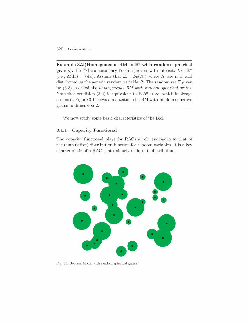
320 Boolean Model
Example 3.2 (Homogeneous BM in Rd with random spherical
grains). Let Φ be a stationary Poisson process with intensity λ on Rd
(i.e., Λ(dx) = λdx). Assume that Ξi = B0(Ri) where Ri are i.i.d. anddistributed as the generic random variable R. The random set Ξ givenby (3.3) is called the homogeneous BM with random spherical grains.Note that condition (3.2) is equivalent to E[Rd] < ∞, which is alwaysassumed. Figure 3.1 shows a realization of a BM with random sphericalgrains in dimension 2.
We now study some basic characteristics of the BM.
3.1.1 Capacity Functional
The capacity functional plays for RACs a role analogous to that ofthe (cumulative) distribution function for random variables. It is a keycharacteristic of a RAC that uniquely defines its distribution.
Fig. 3.1 Boolean Model with random spherical grains.
3.1 Boolean Model as a Coverage Process 321
Definition 3.2. Let Ξ be a RAC. The capacity functional TΞ(K) ofΞ is defined as
TΞ(K) = PΞ ∩ K = ∅for all compacts K ⊂ R
d.
Remark. Obviously, we have TΞ(∅) = 0 and in general 0 ≤ TΞ(K) ≤ 1.These properties can be seen as analogous to the properties F (−∞) =0,0 ≤ F (x) ≤ 1 of a distribution function F of a random variable. Onecan complete the above two properties by another couple of properties,analogous to monotonicity and right continuity of a distribution func-tion, and then define a Choquet alternating capacity functional as anyfunctional T (K) of the compact sets K satisfying the four conditions. Acelebrated theorem of the theory of RACs (Choquet’s theorem; see [29])states that each such capacity functional uniquely defines some RACdistribution, exactly as each d.f. defines the distribution of a randomvariable.
Before calculating the capacity functional of the BM, we prove thefollowing very useful lemma.
Lemma 3.1. Let ΞBM be the BM with intensity of germs Λ and thegeneric grain Ξ. Then, the number of grains of the BM intersecting agiven compact K,
NK = #xi : (xi + Ξi) ∩ K = ∅ ,
is a Poisson random variable with parameter E[Λ(Ξ ⊕ K)].
Proof. Let Φ be a marked Poisson p.p. generating the BM as in Defi-nition 3.1. For a given compact K define the point process
ΦK =∑
(xi,Ξi)∈Φ
εxi ((xi + Ξi) ∩ K = ∅) .
Note that ΦK is an independent thinning of the points of Φ (germs ofthe BM) with the thinning probability
pK(x) = Px + Ξ ∩ K = ∅ = Px ∈ Ξ ⊕ K .

322 Boolean Model
By Proposition 1.8, ΦK is a Poisson p.p. with intensity measurepK(x)Λ(dx). Moreover, NK = ΦK(Rd) is a Poisson random variablewith parameter
∫Rd pK(x)Λ(dx). By Fubini’s theorem∫
Rd
pK(x)Λ(dx) =∫
Rd
Px ∈ Ξ ⊕ K Λ(dx)
= E[∫
Rd
(x ∈ Ξ ⊕ K )Λ(dx)]
= E[Λ(Ξ ⊕ K)] ,
which completes the proof.
We can now calculate the capacity functional of the BM.
Proposition 3.2. The capacity functional of the BM ΞBM with inten-sity of germs Λ and the generic grain Ξ is equal to
TΞBM(K) = 1 − e−E[Λ(Ξ⊕K)] .
Proof. Note that TΞ(K) = PNK = 0, where NK = #xi: (xi + Ξi) ∩K = ∅. The result follows from Lemma 3.1.
3.1.2 Characteristics of the Homogeneous BM
Definition 3.3. We say that the BM ΞBM is homogeneous if theunderlying Poisson p.p. Φ is stationary. The intensity of the latter,0 < λ < ∞, is also called the intensity of the homogeneous BM.
Remark. Note that the distribution of the homogeneous BM is invari-ant with respect to any translation in R
d. Indeed, the homogeneityassumption implies that the capacity functional of ΞBM is translationinvariant, i.e., TΞBM(a + K) = TΞBM(K) for any a ∈ R
d. This followsfrom Proposition 3.2 and the simple observation that |Ξ ⊕ (a + K)| =|a + (Ξ ⊕ K)| = |Ξ ⊕ K|, where |·| denotes Lebesgue measure (volume)

3.1 Boolean Model as a Coverage Process 323
in Rd. The fact that
TΞBM(a + K) = PΞBM ∩ (a + K) = ∅= P(ΞBM − a) ∩ K = ∅= TΞBM−a(K)
and the remark after Definition 3.2 imply that the same holds true forthe distribution of ΞBM.
In the sequel, we will define some important characteristics of aRAC whose distribution is invariant with respect to any translationin R
d (for short, we will speak of a translation invariant RAC) andevaluate these characteristics for the homogeneous BM.
Definition 3.4. (Volume fraction) The volume fraction p of thetranslation invariant RAC Ξ is defined as the mean fraction of thevolume occupied by Ξ
p =E[ |Ξ ∩ B| ]
|B|for |B| > 0, which, by translation invariance of Ξ, can be shown not todepend on the particular choice of bounded B.
Remark. Due to the translation invariance of the RAC, the volumefraction can also be expressed as the probability that a given point (saythe origin) is covered by Ξ. Indeed
p =E[|Ξ ∩ B|]
|B|
=1
|B|∫
BE[ (x ∈ Ξ)]dx
= P0 ∈ Ξ = PΞ ∩ 0 = ∅= TΞ(0),
which is nothing but the capacity functional of Ξ evaluated on asingleton.

324 Boolean Model
By the above remark and Proposition 3.2, we immediately obtainthat:
Corollary 3.3. The homogeneous BM with intensity λ and genericgrain Ξ has the volume fraction
p = 1 − e−λE[ |Ξ| ] .
Definition 3.5. (Covariance function) The covariance functionC(x) of the translation invariant RAC ΞBM is defined as the proba-bility that two points separated by the vector x ∈ R
d belong to ΞBM,i.e., by
C(x) = P0 ∈ ΞBM ,x ∈ ΞBM .
This definition can be extended to any translation invariant RAC.
Note that C(x) = E[ (0 ∈ Ξ) (x ∈ Ξ)], so it is a “non-centered”covariance of the random variables (0 ∈ Ξ) and (x ∈ Ξ); the “true”centered covariance is equal to C(x) − (P(0 ∈ Ξ))2 = C(x) − p2.
If the distribution of the RAC Ξ is invariant with respect to alltranslations and rotations in R
d then C(x) depends only on |x|. In thiscase, we will write C(x) = C(|x|), with a slight abuse of notation.
Corollary 3.4. The covariance function of the homogeneous BM withintensity λ and the generic grain Ξ is equal to
C(x) = 2p − 1 + (1 − p)2eλE[ |Ξ∩(Ξ−x)| ] .
Proof. We write
C(x) = P0 ∈ Ξ ∩ (Ξ − x)= P0 ∈ Ξ + Px ∈ Ξ − P0 ∈ Ξ ∪ (Ξ − x)= 2p − P0 ∈ Ξ ∪ (Ξ − x)= 2p − PΞ ∩ 0,x = ∅= 2p − TΞ(0,x)

3.1 Boolean Model as a Coverage Process 325
= 2p − 1 + e−λE[ |Ξ⊕0,x| ]
= 2p − 1 + e−λE[ |Ξ|+|Ξ−x|−|Ξ∩(Ξ−x)| ]
= 2p − 1 + (1 − p)2eλE[ |Ξ∩(Ξ−x)| ] ,
which completes the proof.
Definition 3.6(Contact distribution function). Consider a trans-lation invariant RAC Ξ. Let B be a given bounded convex set containingthe origin, i.e., 0 ∈ B. The contact distribution function (CDF) HB(r)of Ξ with respect to the test set B is defined as the conditional prob-
ability that the dilation of the set B by the factor r is included in thecomplement Ξc = R
d \ Ξ of the RAC Ξ given 0 ∈ Ξc, i.e.,
HB(r) = PrB ⊂ Ξc |0 ∈ Ξc =PΞ ∩ rB = ∅
1 − p, r ≥ 0 ,
where p is the volume fraction of Ξ.
Different instances of contact distribution functions can be consid-ered, depending on the choice of the test set B. The most popular casesare as follows:
The spherical CDF. This is the case when B = B0(1); in this casethe CDF HB0(1)(r) is the conditional distribution function ofthe distance from 0 to Ξ given 0 ∈ Ξ; see Figure 3.2.
The linear CDF. This case arises when B = [0,v], a segment fromthe origin with direction v ∈ R
d, |v| = 1; in this case the CDFH[0,v](r) is the conditional distribution function of the distancefrom 0 to Ξ in the direction of the vector v, given 0 ∈ Ξ. If Ξ isinvariant with respect to rotations, then the linear CDF doesnot depend on the direction v and H[0,v](r) = H(r) can be seenas the conditional distribution function of the distance from theorigin to Ξ in a randomly chosen direction; see Figure 3.2.
Note that the CDF can be expressed in terms of the capacity func-tional. In particular, the CDF of the homogeneous BM can be evaluatedusing Proposition 3.2.
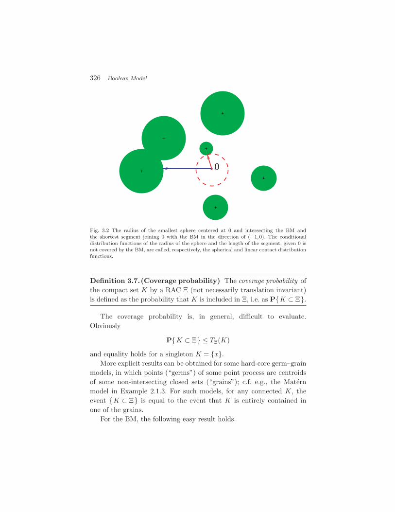
326 Boolean Model
0
Fig. 3.2 The radius of the smallest sphere centered at 0 and intersecting the BM andthe shortest segment joining 0 with the BM in the direction of (−1,0). The conditionaldistribution functions of the radius of the sphere and the length of the segment, given 0 isnot covered by the BM, are called, respectively, the spherical and linear contact distributionfunctions.
Definition 3.7.(Coverage probability) The coverage probability ofthe compact set K by a RAC Ξ (not necessarily translation invariant)is defined as the probability that K is included in Ξ, i.e. as PK ⊂ Ξ.
The coverage probability is, in general, difficult to evaluate.Obviously
PK ⊂ Ξ ≤ TΞ(K)
and equality holds for a singleton K = x.More explicit results can be obtained for some hard-core germ–grain
models, in which points (“germs”) of some point process are centroidsof some non-intersecting closed sets (“grains”); c.f. e.g., the Maternmodel in Example 2.1.3. For such models, for any connected K, theevent K ⊂ Ξ is equal to the event that K is entirely contained inone of the grains.
For the BM, the following easy result holds.

3.1 Boolean Model as a Coverage Process 327
Proposition 3.5. Let ΞBM be the BM given by (3.3) driven by astationary Poisson p.p. with intensity 0 < λ < ∞ and with typical grainΞ. The random set ΞBM covers any given subset K ⊆ R
d of non-nulld-dimensional volume |K| > 0 with probability 1 iff E[ |Ξ| ] = ∞.1
Proof. Assume that the BM covers K for all K with positive volume.Then, by Definition 3.4, its volume fraction is p = 1. Using the explicitformula given in Corollary 3.3, one finds that necessarily E[ |Ξ| ] = ∞.
Conversely, if the latter is true, we have p = 1 and consequentlythe d-dimensional volume of the complement of the BM, R
d \ ΞBM isalmost surely null. In order to conclude that ΞBM covers all K as above,we show that ΞBM = R
d. For this consider the following ε-dilationΞBM(ε) =
⋃i
(xi + (Ξi ⊕ B0(ε))
)of ΞBM, and note that |Rd \ ΞBM| = 0
implies ΞBM(ε) = Rd for any ε > 0. By monotone convergence
PΞBM = Rd = lim
ε→0PΞBM(ε) = R
d = 1 ,
which completes the proof.
More informative results for the coverage of the BM are known onlyin asymptotic form. In this regard, consider the following parametricfamily of homogeneous BMs on the plane R
2 with spherical grains withrandom radius R of finite second moment (cf. Example 3.2).
ΞBM(r) =⋃i
(xi + B0(rRi)) . (3.4)
Proposition 3.6. Let K be a compact set in R2 whose boundary ∂K
has zero 2-D Lebesgue measure, i.e., |∂K| = 0. Consider the family ofBMs (3.4) with intensity of germs λ and assume that E[R2+ε] < ∞ forsome ε > 0. Denote
φ(λ,r) = πr2λE[R2] − log|K|
πr2E[R2]− 2log log
|K|πr2E[R2]
− logE[R]2
E[R2].
1 Strictly speaking, in this case, the set ΞBM is no longer a BM since the condition E[|Ξ|] <∞ is not satisfied; cf. condition (3.2).

328 Boolean Model
Then
PK ⊂ ΞBM(r) = exp[−e−φ(λ,r)] + o(1), as λ → ∞, r → 0 , (3.5)
provided φ(λ,r) tends to some limit (possibly ±∞).
The original proof of the above result (which is very technical andmore general – dimension d ≥ 2, more general grains, and multiple cov-erage – can be found in [25, cf. Lemma 7.3].
Note that the above result gives approximations of the coverageprobability for dense BMs with small grains. The following two partic-ular parameterizations are of interest if one wants to design a BM withsome given (approximate) probability of coverage of a given set K. Thefirst one shows how many germs of a given size are needed, while thesecond one indicates how large grains should be if the density of germsis given.
Corollary 3.7. For a given u (−∞ < u < ∞) take
λ = λ(r)
=1
πr2E[R2]
(log
|K|πr2E[R2]
+ 2log log|K|
πr2E[R2]+ log
E[R]2
E[R2]+ u
)(3.6)
or
r = r(λ) =
√logλ + log logλ + log
(|K|E[R]2/E[R2])
+ u
λπE[R2]. (3.7)
Then
PK ⊂ Ξ = exp[−e−u] + o(1)
as r → 0 or λ → ∞, respectively.
Proof. Note that (3.6) is a solution of the equality φ(λ,r) = u in λ
while (3.7) implies φ(λ,r(λ)) → u when λ → ∞. The result follows fromProposition 3.6.
The following bounds have been shown in [23, Theorem 3.11] in thecase of the BM with grains of fixed (deterministic) radius.

3.2 Boolean Model as a Connectivity Model 329
Proposition 3.8. Let ΞBM(r) be the homogeneous BM given by (3.4)with constant Ri ≡ 1 and intensity of grains λ. Let B = B0(1) denotethe unit disc. Then
1 − min1,3(1 + πr2λ2)e−πr2λ < P
B ⊂
⋃i:xi∈B
(xi + Ξi)
< 1 − 120
min1,(1 + πr2λ2)e−πr2λ.
Note that the above result gives bounds for the probability that theunit disc is included in the union of grains whose germs belong to thisdisc and not to the whole union ΞBM.
The BM is often considered as a model for the total coverageobtained by a deployment of an irregular radio network. One can thinkof an access network, or a sensor network. Points denote locations ofaccess points or sensors, whereas the grains model communication orsensing regions of the antennas. In this context, one can use level setsof the path-loss function (see Section 2.3.1) as these grains.
3.2 Boolean Model as a Connectivity Model
One says that two nodes xi and xj of the BM at (3.3) are connected if(xi + Ξi) ∩ (xj + Ξj) = ∅.
The random geometric graph is the graph associated by Booleanconnectivity: its nodes are the points of the point process and there isan edge between two nodes if they are connected.
Continuum percolation (also referred to as Boolean percolation) isabout the existence of infinite connected components of the BM (orequivalently infinite components in the random geometric graph).
In this section, we restrict our attention to a BM with sphericalgrains.
3.2.1 Connectivity in a Compact Set
Definition 3.8 (Connectivity in a finite window). Given a com-pact set K, we say that the BM ΞBM is connected in K if the set⋃
i:xi∈K(xi + Ξi) is connected.

330 Boolean Model
Only an asymptotic result is known for the probability of the aboveevent in the case of the BM with spherical grains all of the same con-stant radius.
Proposition 3.9. Let K be a square in R2 and consider the parametric
family of BMs ΞBM(r) on R2 given by (3.4) with constant Ri ≡ 1 and
intensity λ. Let φ(λ,r) = 4πr2λ/|K| − logλ. Then
PΞBM(r) is connected in the square K = exp[−e−φ(λ,r)] + o(1) as λ → ∞, r → 0 , (3.8)
provided φ(λ,r) tends to some limit (possibly ±∞).
Proof. We use Proposition 13.4 concerning the Minimal Spanning Tree(MST) of the Poisson p.p. (see Chapter 13). The key observation isthat ΞBM(r) percolates in the square K iff the longest edge MK ofthe minimal spanning tree of Φ ∩ K is not longer than 2r, which isequivalent to
λπM2K − logλ ≤ 4λπr2 − logλ.
Scaling down the radius of the grains and the side of the square K bythe factor
√|K|, we obtain
λπM2 − logλ ≤ 4λπr2/|K| − logλ,
where M is the longest edge of the MST of Φ in the unit square. Theresult now follows from Proposition 13.4.
Corollary 3.10. For a given u (−∞ < u < ∞) take
λ = λ(r) =|K|4πr2
(log
|K|4πr2 + log log
|K|4πr2 + u
)(3.9)
or
r = r(λ) =
√|K|(logλ + u)
4λπ. (3.10)

3.2 Boolean Model as a Connectivity Model 331
Then
PΞBM(r) is connected in the square K = exp[−e−u] + o(1)
as r → 0 or λ → ∞, respectively.
Proof. Note that (3.10) is a solution of the equation φ(λ,r) = u withunknown λ, while (3.9) implies φ(λ(r), r) → u when r → 0. The resultfollows from Proposition 3.6.
3.2.2 Percolation in Rd
In this section, we restrict our attention to homogeneous BMs withspherical grains of random radius R (cf. Example 3.2). Assume thatE[Rd] < ∞. With probability 1 the BM with spherical grains (3.4) isnot connected in R
d. In fact, one can prove the following stronger fact.Denote by νd the volume of a unit-radius ball in R
d. Denote by B0(R0)the grain (ball) centered at 0 under the Palm probability P0 (call it a“typical grain”; cf. Section 2.1.2).
Proposition 3.11. Consider the homogeneous BM ΞBM in Rd given
by (3.4), with r = 1 and intensity λ. Assume that E[Rd] < ∞. Then
• the probability that a typical grain is isolated is equal to
P0
B0(R0) ∩⋃
xi =0
(xi + B0(Ri)
)= ∅
= E[e−λνd
∑dk=0 (d
k)Rd−k0 E[Rk]] , (3.11)
and• the number of isolated grains of ΞBM is infinite with proba-
bility 1.
Proof. Conditioning on the radius R0 = r of the typical grain B0(R0)located at the origin under P0, all other points whose grains are notdisjoint from B0(r) form an independent thinning (cf. Section 1.3.2)
332 Boolean Model
of the marked p.p. Φ′ =∑
i:|xi| =0 ε(xi,B0(Ri)). The retention probabil-ity for position xi and radius Ri is pr(xi,Ri) = Pr + Ri ≥ |xi|. BySlivnyak’s theorem (see Proposition 1.13), under P0, Φ′ is homoge-neous Poisson with intensity λ and by Proposition 1.8, the thinning isa non-homogeneous Poisson p.p. with intensity measure Λ such that
Λ(Rd) = λ
∫Rd
∫R+
pr(x,s)dxF (ds) = λνd
d∑k=0
(d
k
)rd−kE[Rk] := γ(r),
where F is the distribution of R. Consequently, the probability thatB0(r) is isolated is equal to e−γ(r) and (3.11) follows when de-conditioning with respect to the radius R0 = r.
In order to prove the second statement, denote by N = N(Φ) thenumber of isolated grains of the BM ΞBM, where Φ is a Poisson p.p.that generates ΞBM (cf. Definition 3.1). By the ergodicity of the homo-geneous Poisson p.p. (this is easily extended to i.m. Poisson p.p.s; cf.proof of Proposition 1.21), it follows from Proposition 1.22 (4) that N isalmost surely constant. In what follows, we show that N is not bounded,implying N = ∞ almost surely. Indeed, by Campbell’s formula (1.19)and (3.11) we have
E[N(Φ)] = λ
∫Rd
P0B0(R0) is isolated setdx = ∞ ,
which implies that N cannot be bounded.
Remark. From the above considerations it should be clear that evenvery “strange” but possible (i.e., of positive probability) local config-urations of points of the Poisson p.p. can be observed infinitely manytimes in the whole pattern.
We now continue on percolation, which, in view of what was said,cannot be reasonably defined as a total connectivity of ΞBM.
Definition 3.9. The BM percolates on Rd if there exists an infinite
connected component of ΞBM.
Just as with isolated grains, one is also interested in the event that,under the Palm distribution, the typical grain B0(R0) belongs to aninfinite component.

3.2 Boolean Model as a Connectivity Model 333
Remark. By “infinite component” we understand a component whichconsists of an infinite number (#) of grains. Note that such an infinitecomponent is almost surely an unbounded set in the sense that it is notcontained in any bounded window, because the number of grains visiblein a compact window is a.s. finite (as a consequence of E[Rd] < ∞,cf. Lemma 3.1). Denote by C the maximal (in the sense of inclusion)connected subset of ΞBM which includes B0(R0). We call C the clump.
Let our homogeneous BM with spherical grains (see Example 3.2) beparameterized by the intensity λ of the stationary Poisson p.p. Denoteby λc the following “critical” intensity
λc = infλ ≥ 0:P0
λ#C = ∞ > 0
, (3.12)
where #C denotes the number of grains in the clump C and the nota-tion P0
λ makes explicit the dependence of the model on the intensity ofgrains λ.
Remark. Note that the probability P0λ#C = ∞ is increasing in λ.
This can be easily seen using the results on thinning and superpositionof Poisson p.p.s (see Section 1.3). Consequently, P0
λ#C = ∞ = 0 forall 0 ≤ λ < λc (which might be the empty set if λc = 0).
One of the central questions of percolation theory for BMs con-cerns the non-degeneracy of λc (which here means 0 < λc < ∞). Thefollowing “phase transition” type results are known on the matter.
Proposition 3.12. Let λc be the critical intensity (3.12) of the familyof BMs with spherical grains of random radius R.
• If d ≥ 2 and PR0 = 0 < 1 (i.e., if R is not almost surelyequal to 0), then λc < ∞.
• If E[R2d−1] < ∞, then λc > 0.
Remark. For a one-dimensional BM with E[R] < ∞, we have λc = ∞(i.e., #C is almost surely finite for all λ), while if E[R] = ∞ we haveλc = 0: the BM covers the whole line for any λ > 0.2
2 Strictly speaking in this case it is no longer a BM, for which E[R] < ∞ is required; cf.Example 3.2.
334 Boolean Model
Proof. The proof of the finiteness of the critical intensity exploits somediscretization and known results for discrete site percolation (cf. Sec-tion 14.2). Namely, consider some constants η > 0 and p0 > 0, such thatPR ≥ η = p0 > 0; such positive constants exist under the assumptionPR0 = 0 < 1. Consider a square lattice (in R
d) with side of lengthη/(2d
√d). Note that this value is chosen so that any two balls of radius
not less than η, centered at some points of any two adjacent sites of thelattice, are not disjoint. We declare a site of the lattice open if there isa point of Φ in it marked with a ball of radius R ≥ η. Otherwise, wedeclare the site closed. Note that the probability p = p(λ) for a givensite to be open is positive and tends to 1 when λ → ∞. Moreover, thesites are declared open independently. It is known that in this discretemodel with p large enough, but still p < 1, the origin belongs to aninfinite connected set of opened sites with a positive probability; seeProposition 14.5. By the construction of our discrete model, this impliesthat B0(R0) belongs to an infinite connected component with non-nullprobability for λ large enough, thereby ensuring that λc < ∞.
In order to prove that λc > 0, consider the following generationsof grains connected to B0(R0). The first generation consists of all thegrains directly connected to it. Given n ≥ 1 generations, the (n + 1)stgeneration consists of all grains directly connected to some grain ofthe nth generation and which do not intersect any grain of generation1, . . . ,n − 1. We say that any grain xi + B(Ri) is of type k if k − 1 ≤Ri < k (k = 1,2 . . .). Note that the number of grains of type k of the(n + 1)th generation, directly connected to a given grain of type i ofthe nth generation, but not totally contained in it, is not larger thanthe number of all grains of radius R, k ≤ R < k + 1 intersecting thisgiven grain and not totally contained in it, which is in turn dominatedby a Poisson random variable of parameter
µ(i,k) = E[#points of Poisson p.p. in B0(i + k) \B0((i − k)+) marked by R: k ≤ R < k + 1]
= λνd
((i + k)d − (i − k)d
+
)Pk ≤ R < k + 1 .
The process of generations of grains connected to B0(R0) is not abranching process due to the dependence between generations; however

3.2 Boolean Model as a Connectivity Model 335
it can be stochastically bounded by a multi-type branching (Galton–Watson) process with a Poisson number of children of type k bornto a parent of type i; this Poisson number has mean µ(i,k). It is notdifficult to see that the expected number of all individuals in all gener-ations of this branching process, given the root is of type i, is equal to1 +
∑∞n=1∑∞
k=1 mnik, where mn
jk is the jk th entry of the nth power ofthe matrix mik = µ(i,k). It is a matter of a direct calculation (see thedetails in [31, proof of Theorem 3.3]) that the (unconditional) expec-tation of the total number of individuals is finite for sufficiently smallλ > 0 provided E[R2d−1] < ∞.
The critical intensity λc is related to the size of a clump generatedby a typical grain under P0. The following result says that it is alsocritical for percolation as defined in Definition 3.9.
Proposition 3.13. Let λc be the critical intensity (3.12) of the familyof BMs with spherical grains of random radius R.
• Assume λc > 0. If 0 < λ < λc then PλBM percolates = 0.• Assume λc < ∞. If λc < λ then PλBM percolates = 1.• The number of infinite connected components is Pλ-almost
surely constant and equal to 0 or 1.
Proof. Assume 0 < λ < λc. We have by the Campbell formula
PλBM percolates
≤ Eλ
[∑i
(xi ⊕ B0(Ri) belongs to an infinite component
)]
= λ
∫Rd
P0λ#C = ∞dx = 0 .
By the ergodicity of the homogeneous Poisson p.p. (that can be easilyextended to independently marked Poisson p.p.; cf. proof of Propo-sition 1.21), it follows from Proposition 1.22 (4) that the number ofinfinite connected components is almost surely constant.
336 Boolean Model
Assume now that λc < λ < ∞. Note that the BM percolates iff thenumber N of grains which belong to an infinite component is not lessthan 1. As before, it can be shown by the Campbell formula thatEλ[N ] = ∞. Consequently, PλN ≥ 1 > 0, which implies by ergod-icity that PλN ≥ 1 = PλBM percolates = 1.
Proving that the number of infinite connected components is atmost 1 is trickier. The arguments are based on the ergodicity of theBM (see [31, Section 3.6]).
Example 3.3 (Connectivity in ad hoc networks). Consider anad hoc network. Following Example 1.1 we assume that the locationsof the mobile nodes are modeled by some homogeneous Poisson p.p.Φ. Assume that two nodes xi,xj ∈ Φ can communicate directly witheach other if |xi − xj | ≤ ∆, where ∆ is some constant communicationrange. This is equivalent to saying that these nodes are connected inthe BM based on Φ and with spherical grains of radius r = ∆/2 (cf. thedefinition of connectivity at the beginning of Section 3.2). Assume thatthe nodes of this network can relay packets and that multihop routingis used. Then, nodes can communicate through some multihop routeiff they belong to the same connected component of this BM.
A first question concerning the performance of this network concernsits connectivity. One can distinguish two scenarios:
• Limited network case. If we assume a bounded window K
then, it makes sense to ask for the probability of full con-nectivity, i.e., the probability that any two nodes in the net-work can communicate with each other (through a multihoproute). The results of Proposition 3.9 and its corollary canbe used to approximate this probability if the node densityλ is large (i.e., if there are very many nodes in K) and thecommunication range ∆ is small compared to (the side of thesquare) K.
• Large network case. For networks in a large domain, it ismore appropriate to adopt a model based on the BM onthe whole plane (or space). Then, in view of the negativeresult of Proposition 3.11, full connectivity cannot hold and

3.2 Boolean Model as a Connectivity Model 337
the best one can hope for is that a node can communicatewith an infinite number of nodes. In other words, the infinitead hoc network is said to be “connected” if the correspondingBM percolates. Note that in this case, the BM has a uniqueinfinite connected component (Proposition 3.13). The lattercan be interpreted as the “main part” of the network.
We conclude from the above models that one can bring a disconnected(non-percolating) network to the percolation regime by increasing thedensity of nodes or by enlarging the communication range. We shallreturn to this problem in Chapter 8 where we show that this methodfor connecting a network does not always work when interference istaken into account.

4Voronoi Tessellation
4.1 Introduction
In this chapter, we introduce an important random tessellation of theEuclidean space R
d. By definition, a tessellation is a collection of open,pairwise disjoint polyhedra (polygons in the case of R
2), the union ofwhose closures cover the space, and which is locally finite (i.e., thenumber of polyhedra intersecting any given compact set is finite).
Definition 4.1. Given a simple point measure µ on Rd and a point x ∈
Rd, the Voronoi cell Cx(µ) = Cx of the point x ∈ R
d w.r.t. µ is definedto be the set
Cx(µ) = y ∈ Rd: |y − x| < inf
xi∈µ,xi =x|y − xi| .
The Voronoi cell is often defined as the closure of the last set. Given asimple point process Φ =
∑i εxi on R
d, the Voronoi Tessellation (VT)or mosaic generated by Φ is defined to be the marked point process
V =∑
i
ε(xi,Cxi (Φ)−xi) .
338

4.1 Introduction 339
Fig. 4.1 Voronoi tessellation generated by a random sample of points.
The Voronoi cell Cx(µ) as defined above is an open set; it is oftendefined instead as the closure of this set. Observe that, with our def-inition, not every point in R
d is covered by some Voronoi cell: giventwo points xi and xj say of Φ that have Voronoi cells that abut eachother, there are some points y that are common to the boundaries ofboth cells but are not in either (cf. Figure 4.1 which shows the Voronoitessellation generated by some realization of a point process).
Note that the cell Cxi(Φ) of the atom xi is the set of all those pointsof R
d that are closer to this atom xi than to any other atom of Φ.Note also that we consider these cells Cxi − xi shifted to the originas marks of the points xi of Φ. This extends slightly the concept ofmarked point processes considered in Section 2.
One can easily see that each Voronoi cell is a convex polyhedron,but it may be unbounded. It is not difficult to prove, by consideringthe typical cell C0(µ) under the Palm distribution, that in the case of aVoronoi tessellation generated by a homogeneous Poisson p.p., all cellsare bounded with probability 1.
The Voronoi tessellation is an important model for the theory ofpoint processes as well as for applications. In the remaining part ofthis chapter, we will show it “in action” in a few theoretical and morepractical contexts.
340 Voronoi Tessellation
4.2 The Inverse Formula of Palm Calculus
In Section 1.6 (and in more detail in Chapter 10) we defined the Palm–Matthes distribution P0 of a stationary point process Φ; it can beinterpreted as the conditional distribution of Φ given Φ(0) ≥ 1. Wewill now show how the stationary distribution P of Φ can be retrievedfrom P0 using Voronoi cells.
Theorem 4.1. Let Φ be a simple stationary point process with inten-sity 0 < λ < ∞. For all non-negative functions f :M → R
+,
E[f(Φ)] = λE0[∫
Rd
f(Φ − x) (x ∈ C0(Φ))dx
].
Proof. Let us take
h(x,Φ) =(Φ(B
0(|x|)) = 0),
where Bx(r) = y: |y − x| < r is the open ball of radius r centered at
x. Let us take for granted the property (proved below in Lemma 4.2)that among the points of Φ, with probability 1 w.r.t. P, there is aunique point which is closest to the origin. Using this property, we canstate that with probability 1,∫
Rd
h(x,Φ)Φ(dx) = 1 ,
and consequently by the Campbell–Matthes formula (1.19) (see alsoSection 10.2.2),
E[f(Φ)] = E[∫
Rd
f(Φ + x − x)h(x,Φ + x − x)Φ(dx)]
= λ
∫Rd
E0[f(Φ + x)h(x,Φ + x)]dx
= λ
∫Rd
E0[f(Φ − x)h(−x,Φ + x)]dx
= λE0[∫
Rd
f(Φ − x) (x ∈ C0(Φ))dx
].
4.2 The Inverse Formula of Palm Calculus 341
It remains to prove:
Lemma 4.2. For a simple stationary non-null point process Φ
Pthere exist two or more distinct points
equidistant to the origin 0 = 0 .
Proof.
Pthere exist two or more distinct points equidistant to the origin
≤ E[∫
Rd
(Φ(y = x : |y| = |x|) ≥ 1
)Φ(dx)
]≤ E
[∫Rd
((Φ − x)(y′ = 0 : |y′ + x| = |x|) ≥ 1
)Φ(dx)
]= λE0
[∫Rd
(Φ(y′ = 0 : |y′ + x| = |x|) ≥ 1
)dx
]≤ λE0
[∫Rd
∫Rd\0
(|y′ + x| = |x|)Φ(dy′)dx
]= λE0
[∫Rd\0
‖x : |y′ + x| = |x|‖Φ(dy′)]
= 0,
where ‖ · ‖ denotes the d-dimensional volume.
Let us now take f ≡ 1; this yields the following formula, which deter-mines the mean value of the volume of the typical cell:
Corollary 4.3.
1 = λE0[|C0(Φ)|].
There are no closed form expressions for the distribution of thevolume of the typical cell except for dimension 1.
Let us call now C(0,Φ) the cell of the stationary tessellation Vthat covers the origin (i.e., 0 ∈ C(0,Φ)). In view of Lemma 4.2, C(0,Φ)is uniquely defined for almost all realizations of Φ w.r.t. P. Let us

342 Voronoi Tessellation
take f = g(C(0,Φ)) if C(0,Φ) is unique and 0 if not, where g is somenon-negative function of C(0,Φ) (e.g., its volume, perimeter, numberof sides, etc.). We obtain the following corollary.
Corollary 4.4.
E[g(C(0,Φ))] = λE0[g(C0(Φ))|C0(Φ)|] .In particular,
E[
1|C(0,Φ)|
]=
1E0[|C0(Φ)|] .
By Jensen’s inequality, one obtains the following result that can beseen as yet another incarnation of the waiting time paradox (see [14],Vol. 2)
E[|C(0,Φ)|] ≥ E0[|(C0(Φ)|] .This paradox is explained by the fact that the cell which covers theorigin is sampled with some bias with respect to the distribution ofthe typical cell C0(Φ) under P0, namely, this sampling favors large cells(as having more chance to cover a given fixed point). For more on thisbias, see e.g., [33].
The next example shows how Theorem 4.1 can be used to constructa stationary periodic point process.
Example 4.1 (Stationarization of the honeycomb). Consider aregular hexagonal grid on R
2 with the distance ∆ between two adja-cent vertexes of this grid. (The set of vertexes of this grid canbe described on the complex plane by Hex = ∆(u1 + u2eiπ/3), u =(u1,u2) ∈ 0,±1, . . .2). Consider a (deterministic) point process ΦHex
whose points are located on this grid. Consider this deterministic sce-nario as the Palm distribution P0 of some stationary point process.Note that the surface area of the typical cell (hexagon) of this pro-cess is equal to ∆2/(2π
√3). Thus its intensity is λHex = 2π
√3/∆2. By
Theorem 4.1, the stationary version of this periodic p.p. can be con-structed by randomly shifting the deterministic pattern Hex through a
4.3 The Neveu Exchange Formula 343
vector uniformly distributed in the Voronoi cell (hexagon) of the origin.The Voronoi tessellation generated by this (Palm or stationary) p.p. issometimes called the honeycomb model.
4.3 The Neveu Exchange Formula
In this section, we will prove another useful formula of the Palm calculusconnecting the Palm distributions of two stationary point processes.Again, the Voronoi tessellation will be used as a tool. The formalism forPalm probabilities is that defined in Remark 10.1 which allows one todefine several Palm probabilities on a common probability space thatcarries several point processes. The key tool is again the Campbell–Matthes formula that in the case of two stationary (not necessarilyindependent!) point processes has the following incarnation
E[∫
Rd
g(x,Φ − x,Φ′ − x)Φ(dx)]
= λ
∫Rd
E0[g(x,Φ,Φ′)]dx, (4.1)
where λ < ∞ is the intensity of Φ and E0 is the expectation with respectto its Palm probability P0; i.e., in particular, P0Φ(0) ≥ 1 = 1.
Theorem 4.5 (Exchange formula). Let Φ and Φ′ be two simplestationary point processes (defined on the same probability space) withintensity, respectively, 0 < λ < ∞ and 0 < λ′ < ∞. Let E0
Φ and E0Φ′
denote the Palm–Matthes probabilities of Φ and Φ′, respectively. If
E0Φ′[Φ(∂C0(Φ′))
]= 0, (4.2)
where ∂ denotes the boundary, then for any non-negative functionf(φ,φ′) of the point measures (φ,φ′) we have
λE0Φ[f(Φ,Φ′)
]= λ′E0
Φ′
[∫Rd
f(Φ − x,Φ′ − x)(x ∈ C0(Φ′)
)Φ(dx)
].
Proof. It suffices to prove the formula for a bounded function, soin what follows we assume that supf ≤ 1. For any x ∈ R
d let Fx =Fx(Φ,Φ′) = f(Φ − x,Φ′ − x). By the Campbell formula (4.1) (see also
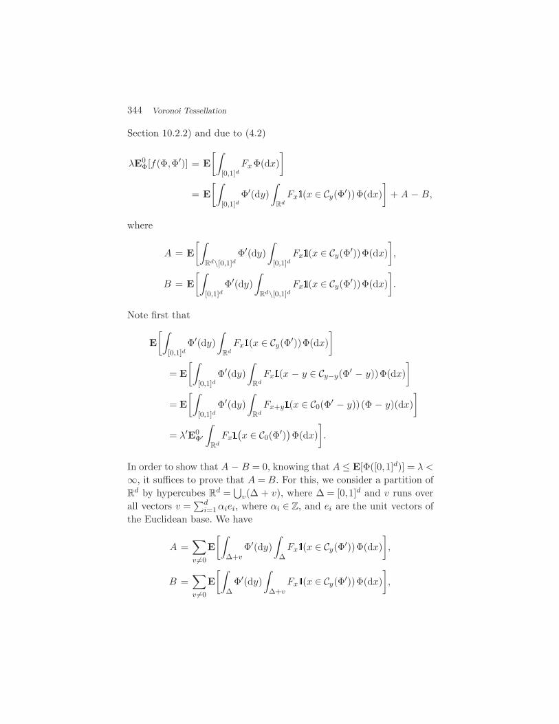
344 Voronoi Tessellation
Section 10.2.2) and due to (4.2)
λE0Φ[f(Φ,Φ′)] = E
[∫[0,1]d
Fx Φ(dx)]
= E[∫
[0,1]dΦ′(dy)
∫Rd
Fx (x ∈ Cy(Φ′))Φ(dx)]
+ A − B,
where
A = E[∫
Rd\[0,1]dΦ′(dy)
∫[0,1]d
Fx (x ∈ Cy(Φ′))Φ(dx)],
B = E[∫
[0,1]dΦ′(dy)
∫Rd\[0,1]d
Fx (x ∈ Cy(Φ′))Φ(dx)].
Note first that
E[∫
[0,1]dΦ′(dy)
∫Rd
Fx (x ∈ Cy(Φ′))Φ(dx)]
= E[∫
[0,1]dΦ′(dy)
∫Rd
Fx (x − y ∈ Cy−y(Φ′ − y))Φ(dx)]
= E[∫
[0,1]dΦ′(dy)
∫Rd
Fx+y (x ∈ C0(Φ′ − y))(Φ − y)(dx)]
= λ′E0Φ′
∫Rd
Fx
(x ∈ C0(Φ′)
)Φ(dx)
].
In order to show that A − B = 0, knowing that A ≤ E[Φ([0,1]d)] = λ <
∞, it suffices to prove that A = B. For this, we consider a partition ofR
d by hypercubes Rd =⋃
v(∆ + v), where ∆ = [0,1]d and v runs overall vectors v =
∑di=1 αiei, where αi ∈ Z, and ei are the unit vectors of
the Euclidean base. We have
A =∑v =0
E[∫
∆+vΦ′(dy)
∫∆
Fx (x ∈ Cy(Φ′))Φ(dx)],
B =∑v =0
E[∫
∆Φ′(dy)
∫∆+v
Fx (x ∈ Cy(Φ′))Φ(dx)],
4.4 Neighbors in the Voronoi Tessellation, Delaunay Triangulation 345
and for each v = 0,
E[∫
∆+vΦ′(dy)
∫∆
Fx (x ∈ Cy(Φ′))Φ(dx)]
= E[∫
∆(Φ′ − v)(dy)
∫∆
Fx (x ∈ Cy+v(Φ′))Φ(dx)]
= E[∫
∆(Φ′ − v)(dy)
∫∆
F − x (x ∈ Cy(Φ′ − v) + v)Φ(dx)]
= E[∫
∆(Φ′ − v)(dy)
∫∆
Fx (x − v ∈ Cy(Φ′ − v))Φ(dx)]
= E[∫
∆(Φ′ − v)(dy)
∫∆−v
Fx+v (x ∈ Cy(Φ′ − v))(Φ − v)(dx)]
= E[∫
∆Φ′(dy)
∫∆−v
Fx (x ∈ Cy(Φ′))Φ(dx)],
where the last equality is due to the stationary of both point processes.Thus A = B, which concludes the proof.
4.4 Neighbors in the Voronoi Tessellation, DelaunayTriangulation
Let Cx(µ) be the Voronoi cell of x ∈ Rd generated by the point pattern
µ that is always assumed in this section to be simple (µ(z) = 0 or 1).We will call any point y ∈ µ such that y = x and |a − x| = |a − y| forsome a ∈ Cx(µ), where Cx(µ) denotes the closure of Cx(µ), a Voronoineighbor of x.
Definition 4.2. The Delaunay triangulation generated by a simplepoint measure µ is a graph with the set of vertices µ and edges con-necting each y ∈ µ to any of its Voronoi neighbors.
Example 4.2 (Neighborhood in ad hoc networks). In a periodic(say hexagonal or square) grid, it is obvious to define the neighbors of agiven vertex. However, for irregular patterns of points like a realizationof a Poisson p.p., which we use below to model the set of nodes of ad hoc
346 Voronoi Tessellation
networks (cf. Example 1.1), this notion is less evident. The Delaunaytriangulation offers some purely geometric definition of ‘neighborhood’in such patterns.
Define, for x ∈ Rd,
Nx(µ) =y ∈ µ : µ
(B(x,y,z)
)= 0
for some z = z1, . . . ,zd−1 ∈ µ, x,y,zi, distinct,
where B(x,y,z) is the open ball circumscribed on the points x,y,zi.The following geometric result allows us to identify the Voronoi neigh-bors of x in µ or equivalently the edges from x in the Delaunay trian-gulation:
Lemma 4.6. Assume that Cx(µ) is bounded. Then, for x in µ, Nx(µ)coincides with the set of Voronoi neighbors of x.
Proof. Define a vertex of the cell Cx(µ) to be any location in z ∈ Rd
equidistant to x and (at least) d − 1 other points y1, . . . ,yd−1 ∈ µ. Weuse below the fact that if z is such a vertex, then each of the pointsy1, . . . ,yd−1 is a Voronoi neighbor of x.
If y ∈ µ belongs to Nx(µ), then by definition, there exists an emptyopen ball with x,y,z1, . . . ,zd−1 on its boundary, where z1, . . . ,zd−1 ∈ µ.So, the center of this ball is a vertex of the cell Cx(µ) and therefore, y
is a Voronoi neighbor of x.Conversely, if y is a Voronoi neighbor of x, since the cell Cx(µ) is
finite, its boundary contains a finite domain Dd1 included in the hyper-plane of dimension d − 1 equidistant to x and y; the boundaries ofDd1 are finite domains contained in hyperplanes of dimension d − 2.Let Dd−2 be one of the latter. There exists a triple of points (x,y,z1)which are equidistant to any element of the Dd−2. More generally, forall 2 ≤ k ≤ d − 1, there exists a finite domain Dd−k included in somehyperplane of dimension d − k and such that all the elements of Dd−k
are equidistant to (x,y,z1, . . . ,zk−1) for some z1, . . . ,zk−1 ∈ µ. In par-ticular, there exists a location z of the boundary of Cx(µ) and pointsz1, . . . ,zd−1 ∈ µ such that z is equidistant to x, y and z1, . . . ,zd−1. Thatis y ∈ Nx(µ).

4.5 The Voronoi Tessellation Model for Cellular Access Networks 347
The open ball centered at a vertex of Cx(µ) and having x on itsboundary is empty of points of µ. The union of these balls over allvertexes of the cell is called the fundamental region (or the Voronoiflower) of the cell Cx(µ). It is easy to see that the Voronoi flowercontains the Voronoi cell.
Proposition 4.7. Assume that Cx(µ) is bounded. Then the Voronoiflower of Cx(µ) is a random stopping set.
Proof. For a given compact set K, consider balls centered at thevertexes of Cx(µ) with radii growing until they hit x or any ofthem hits the complement Kc of K. Use a similar argument as inExample 1.10.
4.5 The Voronoi Tessellation Model for Cellular AccessNetworks
We give an example of VT based model of cellular access networks (seeSection 25.3.2 in Volume II) which will be used later.
Example 4.3 (Cellular Access Network). The model componentsare as below:
• Users and Access Points located on the plane R2 are rep-
resented by two independent stationary point processes,denoted, respectively, by Φu and Φa.
• Each access point xi ∈ Φa serves users in a geographical zonewhich is modeled by its Voronoi cell Cxi(Φa). Note that thisassumption is equivalent to the hypothesis that each user isserved by the nearest access point.
• The model parameters are the intensities λu,λa of the p.p.sΦu,Φa, respectively. Typically λu > λa, but this assumptionis not essential for our analysis.
Consider now the following mean additive characteristic associated withthe typical cell of the access network model:
I = E0Φa
[∫R2
(x ∈ C0(Φa))g(x,Φa)Φu(dx)],

348 Voronoi Tessellation
where E0Φa
is the expectation w.r.t the Palm distribution of Φa and g
is a non-negative function of the location x ∈ R2 and the pattern Φa
of access points. Taking different functions g, one gets the followingexamples of such additive characteristics:
• if g(x,φ) ≡ 1, then I = M represents the mean number ofusers in the typical cell;
• if g(x,φ) = |x|, then I = L is the mean total length of connec-tions in this cell (which is more pertinent in a wired accessnetwork);
• if g(x,φ) = 1/l(|x|), where l(r) is some omni-directional path-loss function as considered in Example 23.3 in Volume II,then I = P represents the mean total power received by theaccess point from all the users attached to it (assuming allusers transmit with a constant power 1);
• if g(x,φ) = l(|x|) with l(·) as above, then I = (PL) representsthe mean total path-loss “received” at the access point fromall the users it serves;
• if g(x,φ) = l(|x|)∑yi∈φ 1/l(|x − yi|) with l(·) as above, thenI = (RPL) represents the mean total relative path-loss ratio“received” at the access point from all its users.
Let h(x,Φ) be defined as in the proof of Theorem 4.1 and take
f(Φu,Φa) = f(Φa) =∫
R2g(−y,Φa − y)h(y,Φa)Φa(dy) .
Recall from the definition of h that f(Φa) = g(−Y ∗,Φa − Y ∗) whereY ∗ = arg min|yi|:y ∈ Φa is the access point nearest to the origin (a.s.uniquely defined due to stationarity and the fact that the p.p. is simple).Moreover, on the set Φa(0) ≥ 1 for x ∈ C0(Φa) we have f(Φa −x) = g(x,Φa). Thus, by Neveu’s exchange formula (Theorem 4.5) weobtain that
I =λu
λaE0
Φu
[g(−Y ∗,Φa − Y ∗)
]. (4.3)
We see that the Neveu exchange formula allows us to transform the“access-point centric” scenario into a dual “user-centric” scenario. This
4.5 The Voronoi Tessellation Model for Cellular Access Networks 349
transformation shows that the mean number of users per access point(case g(x) ≡ 1) is equal to
M =λu
λa.
When Φa is a Poisson p.p. one can explicitly evaluate (4.3) for varioustypes of additive characteristics. Under Poisson assumptions (for Φa
only) one knows the distribution function of Y ∗, namely P0Φa
|Y ∗| >
r = P0Φa
Φa(B0(r)) = 0 = exp[−λaπr2], and it is not difficult to seethat the argument ∠(Y ∗) is uniformly distributed on [0,2π). More-over, given |Y ∗| = r, all points of Φa which are farther away from 0than r form a non-homogeneous Poisson p.p. with intensity measureλa (|y| > r)dy (see Section 1.5). We denote this Poisson process byΦa|>r. Consequently
I =λu
λa
12π
∫ 2π
0
∫ ∞
0rE[g((r cosθ,r sinθ),Φa|>r
)]e−λaπr2
drdθ . (4.4)
For g(x,φ) = |x|, we obtain
L =λa
2λ3/2c
.
The mean received power P with l(r) given by OPL 1 or OPL 2in Example 23.3 in Volume II can be given in terms of some specialfunctions (note that for OPL 3, I = ∞ due to the pole at the origin).The mean path-loss expression is explicit and, for OPL 3, it takes theform
(PL) =λu
λa
AβΓ(1 + β/2)(λaπ)β/2 .
Under the same assumption, the mean relative path-loss is equal to
(RPL) =λu
λa
2β − 2
.

Bibliographical Notes on Part I
Chapters 1 and 2 cover classical topics in point process theory. A clas-sical reference on the matter is [9]. Most results are well known. Theapproach of Section 1.5 is borrowed from [46]. For more on hard-spherepacking problems mentioned in Example 2.1.3, see e.g., [8]. We did notfind references for the discussion of Example 1.4 but it is likely thatthese simple observations were already made.
Shot noise processes and Boolean models as considered in Chap-ters 2 and 3 respectively, are core topics in stochastic geometry. For acomprehensive treatise on the matter, see [42]. For an analysis of thetail behavior of Shot Noise fields, the reader might consult [17]. For ahistory on the use of Shot Noise fields to represent interference, see theintroductory paper of [22]. We did not find earlier papers on the jointdistribution of the time–space SN proposed in Section 2.3.4.
For the class of random tessellations discussed in Chapter 4, thereader could consult [33]. For a general book on tessellations, see [34].The models of Section 4.5 come from [3] and [2]. For a recent surveyon the matter, see [47].
Point processes and stochastic geometry models are widely used inspatial statistics; see, e.g., [24] for a recent book on this subject.
350

Part II
Signal-to-InterferenceRatio Stochastic
Geometry

352
This part bears on stochastic geometry models defined by SINR.More precisely, we define and analyze a random coverage process of thed-dimensional Euclidean space which stems from the wireless commu-nication setting described in Part VI in Volume II. As for the Booleanmodel, the minimal stochastic setting consists of a point process onthis Euclidean space and a sequence of real-valued random variablesconsidered as marks of this point process. In this coverage process, thecell attached to a point is defined as the region of the space where theeffect/response of the mark of this point exceeds an affine function ofthe shot-noise process associated with the other points of the markedpoint process.
Chapter 5 describes the typical cell: its volume, its shape, etc. Chap-ter 6 focuses on the interaction between cells within this setting. Chap-ter 7 studies the coverage process created by the collection of SINRcells. Finally, Chapter 8 studies the connectivity of this coverage pro-cess and in particular the conditions under which it percolates.

5Signal-to-Interference Ratio Cells
5.1 Introduction
Let Φ =∑
i ε(xi,mi) be a marked point process, with points xi in Rd
and marks mi in R. Consider a scalar shot-noise field IΦ(y) defined
on the same space as Φ (i.e. on Rd), and generated by Φ and by the
response function L:Rd × Rd × R
→ R+ (cf. Section 2.2). Let w(y) ≥ 0
be some external or thermal noise field.
Definition 5.1. We define the Signal to Interference and Noise Ratio(SINR) cell of point (X,M) for threshold t ≥ 0 as
C(X,M) = C(X,M)(Φ,w,t) =y ∈ R
d:L(y,X,M) ≥ t(IΦ(y) + w(y)
).
(5.1)
For more on the physical meaning of SINR, see Section 24.3.4 inVolume II.
Example 5.1. (Bit-rate level sets in interference and noisefield) The simplest scenario is that where the mark of point X is thepower P ∈ R
+ emitted by the antenna located at X ∈ R2 and where
353

354 Signal-to-Interference Ratio Cells
L(y,x,P ) = P/l(|x − y|), with l the mean omni-directional path-lossfunction (see Section 23.1.2 in Volume II). More general scenarios canbe described with richer marks (such as antenna azimuth, fading, etc.).Other cases of interest are those where some interference and/or noisecancellation techniques are used. This results in models where the cellis defined with a more general affine function:
C(X,M) = C(X,M)(Φ,w,t) =y ∈ R
d:L(y,X,M) ≥ t(κIΦ(y) + γw(y)
)(5.2)
where κ and γ are factors smaller than one (cf. Section 24.3.4 in Vol-ume II where we discuss the case γ = 1 and κ small in Equation (24.20in Volume II).
Then C(X,P ) represents the set of locations y where the SINR ofthe channel from X to y is larger than the threshold t as illustrated byFigure 5.1.
Within the setting of Section 24.3.4 in Volume II, this translatesinto some bit-error probability, and consequently into some channelgoodput. The exact relation between t and the bit-rate depends onparticular modulation and coding used.
φ y>
+ I ( )
x1
x2
w
x3
x
x4
5
l(y−x)
xPy
P/ l(y−x)
wt
Fig. 5.1 Location y belongs to the cell C of point x because the SINR from x exceeds t at y.The cell C is the set of locations of the plane where a minimum bit rate can be guaranteedfrom transmitter x.

5.2 The Signal-to-Interference Ratio Cell is Well-Defined 355
Some instances of SINR cells are given in Figures 5.2, 5.3, 5.4, 7.1.Notice that the SINR cell C(X,P ) is not always a convex set. In somecases it can even be not connected.
5.2 The Signal-to-Interference Ratio Cell is Well-Defined
There are two levels at which the definition of the SINR cell can betreated.
Firstly, recall from Section 2.2 that the shot-noise field with non-negative response function is always well defined but may be infinite.At a second, more theoretical level, one may ask whether the SINR cell,which is a random set, is almost surely a closed set. This is a naturalquestion in stochastic geometry, where the space of closed sets is astandard observation space for random objects. The following result,which immediately follows from Proposition 2.5 gives some sufficientconditions for this to hold.
Corollary 5.2. Let Φ be an i.m.p.p. Assume that the thermal noisew(y) has almost surely continuous trajectories. If L(y,x,m) is con-tinuous in y and if for each y ∈ R
d, there exists a ball B(y,εy) suchthat (2.15) holds, then IΦ(y) is almost surely finite and has continuoustrajectories. Consequently the SINR cell C(X,M)(Φ,w,t) is a (random)closed set with probability 1.
5.3 Standard Stochastic Scenario and First Order CellCharacteristics
Following the assumptions of Section 2.3.1, we will often consider thefollowing standard stochastic scenario for SINR cells:
(1) Φ is a general stationary i.m.p.p. with points in R2 and inten-
sity λ > 0;(2) the marks pi have a distribution Pp ≤ s = G(s) that does
not depend on the location of the point;(3) The mark M = P of the point X generating the cell C(X,P )
is independent of Φ and has also distribution function G.
356 Signal-to-Interference Ratio Cells
(4) The thermal noise field w(y) = W is constant in space andequal everywhere to some non-negative random variableW ≥ 0 independent of Φ and P .
A slightly more general case is that where:
(3′) the mark M = P of the point X generating the cell C(X,P )
is independent of Φ but has a different distribution functionG′ than the marks of the point process.
Remark. More general scenarios are considered in other chapters. Forinstance power control, studied in Chapter 19 in Volume II, requirespowers which are dependent marks of the p.p.; similarly, the case ofspace and/or time dependent thermal noise is studied in Chapter 17 inVolume II.
Kendall-like Notation cont. Developing our previous Kendall-likenotation for SN (see Section 2.3.1), we call the above scenario the
GIW+GI/GI model, where the GI in the numerator denotes a general dis-tribution for P and the GI/GI in the denominator denotes the SNinterference model. Special cases of distributions are deterministic (D)and exponential (M). We recall that M/· denotes an SN model with aPoisson point process.
This contains two important particular cases:
• The GI0+GI/GI model, which will be referred to as the interfer-
ence limited model (since the thermal noise is not present);
• The GIW+0 model, where the interference is absent, and which
will be referred to as the noise limited model, and which boilsdown to the Boolean (or to the conditional Boolean) modelunder natural assumptions on the attenuation function (seeSection 5.5).
5.3.1 One Point Coverage Probability
Assume the standard SINR cell scenario of Section 5.3. We are inter-ested in the probability that the SINR cell C(X,P ) generated by a point

5.3 Standard Stochastic Scenario and First Order Cell Characteristics 357
located, say, at the origin X = 0, covers a given location y; i.e.,
p0(y) = P
y ∈ C(0,P )(Φ,W,t)
= P
P ≥ l(|y|)t(W + IΦ(y))
.
(5.3)Note that this probability is the value of the capacity functionalTC(0,P )(y) of the random (assume closed) set C(0,P ) evaluated on thesingleton y (cf. Definition 3.2).
Here is a general result for the GIW+GI/GI case.
Proposition 5.3. Assume the GIW+GI/GI standard scenario of Sec-
tion 5.3 with condition (3′) (i.e. P can have a distribution which differsfrom that of the marks of Φ). Assume the following:
• at least one of the random variables W,IΦ or P has a Fouriertransform which is square integrable;
• each of the random variables W,IΦ and P has a finite firstmoment.
Let
η(ξ) = E[exp(−2iπξIφ(y))]E [exp(−2iπξW )]
×E [exp(−2iπξP/(tl(|y|)))] . (5.4)
Then
p0(y) =12
− 12iπ
∫ ∞
−∞η(ξ)ξ
dξ , (5.5)
where the singular contour integral in the right-hand side, which has apole at ξ = 0, is understood in the principal value sense; i.e., one hasto calculate this integral over the domain (−∞,−ε] ∪ [ε,∞) and thenlet ε decrease to 0.
Proof. Since X is the sum of independent random variables, it sufficesthat one of the terms of the sum has a density for X to have one.If this density has a square integrable Fourier transform, so does X. Ifall terms in the sum have finite first moments, so has X. The resultfollows from applying Corollary 12.4 in the Appendix to the density ofthe random variable X = P/(tl(|y|)) − W − IΦ(y).

358 Signal-to-Interference Ratio Cells
The above proposition is useful when one knows the Fourier trans-form of the shot-noise IΦ. This is the case in particular for the M/GISN; i.e, when Φ is an i.m. Poisson p.p. (and more generally some dou-bly stochastic Poisson process). Indeed, E[e−2iπξIΦ ] = LIΦ
(2iπξ) andthe Laplace transform LIΦ
of the Poisson shot-noise is known in closedform (see Proposition 2.6 and Example 2.2).
Some sufficient conditions for IΦ(y) to have a density are given inProposition 2.8.
There are several interesting cases where the shot-noise IΦ has aninfinite mean. Even in the M/GI SN case, this is the case when oneadopts the OPL 3 attenuation model (see Remark 2.4 of Chapter 2).For such scenarios, the assumptions of the last proposition do not hold.We can then use the following result.
Proposition 5.4. Assume the GIW+GI/GI standard scenario of Sec-
tion 5.3 with condition (3′) (i.e. P can have a distribution which differsfrom that of the marks of Φ). Assume the following:
• at least one of the random variables W,IΦ has density witha Fourier transform which is square integrable;
• the random variable P has density with a Fourier transformwhich is square integrable;
• the random variable P has a finite first moment.
Then
p0(y) =∫
R
E[exp(−2iπξIΦ(y))
]E [exp(−2iπξW )]
×E [exp(−2iπξP/(tl(|y|)))] − 12iπs
ds. (5.6)
Proof. The proof follows immediately from Equation (5.3) above andCorollary 12.2 in the Appendix.
Proposition 5.5. For the MW+GI/GI model
p0(y) = LW
(µtl(|y|))LIΦ
(µtl(|y|)) ,
where LW is the Laplace transform of W .

5.3 Standard Stochastic Scenario and First Order Cell Characteristics 359
Proof. We have
p0(y) = P
P ≥ tl(|y|)(W + IΦ)
=∫ ∞
0e−µutl(|y|)FW+IΦ
(du)
= LW
(µtl(|y|))LIΦ
(µtl(|y|)),
where the last equality relies on the fact that the Laplace transformof the sum of independent random variables is equal to the product ofthe Laplace transforms of the terms.
Example 5.6. For M0+M/M model with OPL 3 and W = 0,
p0(y) = e−λ|y|2t2/βK , where K = K(β) =(2πΓ(2/β)Γ(1 − 2/β)
)/β.
Example 5.7. Consider the PHW+GI/GI model, where PH means that P
has the phase-type distribution PH(α,B, b). Recall that it is defined asthe distribution of the time until absorption of the pure-jump Markovchain on the state space 0,1, . . . , b with infinitesimal generator B(which is a (b + 1) × (b + 1)-matrix), where 0 is an absorbing state andwhere α is the vector describing the initial distribution on 1, . . . , b.The tail-distribution function of P is known to be equal to
PP ≥ u = αeuB = α
∞∑n=0
unBn
n!,
where eB is the matrix exponential defined by the corresponding powerseries. For this model, we have
p0(y) =∫ ∞
0PP ≥ tl(|y|)uP(W + I = du)
=∫ ∞
0α
∞∑n=0
(utl(|y|)B)n
n!P(W + I = du)
360 Signal-to-Interference Ratio Cells
= α
∞∑n=0
(tl(|y|)B)n
n!
∫ ∞
0un P(W + I = du)
= α
∞∑n=0
(tl(|y|)B)n
n!E[(W + I)n].
Note that for the M/G SN model, the moments of the shot-noise canbe obtained from the closed form expression of the Laplace transform.Hence it is possible to evaluate (at least numerically) all terms of theabove expansion.
5.3.2 Mean Cell Volume
The one-point coverage probability is related to the mean cell volumeby the following simple relation:
v0 ≡ E[|C(0,P )|
]= E
[∫ (y ∈ C(0,P )
)dy
]=∫
p0(y)dy . (5.7)
Example 5.8. For the M0+M/M model with OPL 3
v0 ≡ E[|C(0,P )|
]=
1λt2/β
β
2Γ(2/β)Γ(1 − 2/β).
5.4 Fading in Signal-to-Interference Ratio Cell and HigherOrder Characteristics
A simple higher order characteristic of a random closed set is its covari-ance function defined as the two-point coverage probability Py1 ∈C(0,P ),y2 ∈ C(0,P ) for two given points y,z (cf. Definition 3.5). In gen-eral, it is difficult to evaluate this probability analytically even for the
MW+M/M model. A special, but very important case, is when the fadingis appropriately taken into account in the SINR cell model.
We have seen in Section 2.3.3 that a precise description of realityrequires a response function of the form L(x,y,p) = pF (x,y)/l(|x − y|)where F (x,y) is a random fading field on R
2 × R2.
Moreover, in Section 2.3.3.2 we have introduced the GI/GI/kmodel for SN, which is useful when a discrete number of receiver

5.4 Fading in Signal-to-Interference Ratio Cell and Higher Order Characteristics 361
locations yj , j = 1, . . . ,k is involved. In this model, instead of consider-ing the whole fading field, one attaches a k-dimensional fading vector(f1
i , . . . ,fki ) to each point of the point process, where (f1
i , . . . ,fki ) rep-
resents the channel conditions f j = F (xi,yj), in the channels from theconsidered point towards the k receivers. Now we adopt this approachin the SINR cell model.
Kendall-like Notation cont. We consider the GI/k/(W +GI/GI/k) model, where the k in the numerator means that the markattached to point X consists of the emitted power P and a fadingvector (F 1, . . . ,F k), with F j = F (X,yj), describing the channels fromX to k locations y1, . . . ,yk. The notation GI/GI/k in the denominatormeans that the fading conditions are taken into account for all inter-fering signals as well. In this model, we assume that all fading variablesare independent.
5.4.1 Covariance Function
We now analyze the covariance function p0(y1,y2) = Py1 ∈ C(0,P ),y2 ∈C(0,P ) of the SINR cell with fading.
Proposition 5.9. For the M/2W+GI/GI/2 model, we have
p0(y1,y2) = LW
(µt(l(|y1|) + l(|y2|)
))L(I1,I2)(µtl(|y1|),µtl(|y2|)
),
where L(I1,I2)(t1, t2) is the joint Laplace transform of the vector(I1, I2) = (IΦ(y1), IΦ(y2)) of the SN in the GI/GI/2 model.
Proof. When using the same type of arguments as in the proof of Propo-sition 5.5, we have
p0(y1,y2) = P
PF1 ≥ tl(|y1|)(W + I1), PF2 ≥ tl(|y2|)(W + I2)
=∫ ∞
0
∫ ∞
0
∫ ∞
0e−µut(l(|y1|)+l(|y2|))e−µv1tl(|y1|)e−µv2tl(|y2|)
×P(W = du,I1 = dv1, I2 = dv2
)= LW
(µt(l(|y1|) + l(|y2|)
))L(I1,I2)(µtl(|y1|),µtl(|y2|)
),
362 Signal-to-Interference Ratio Cells
where the first equality uses the fact that in the M/2 model, the receivedpowers PF1,PF2 are independent exponential random variables withparameter µ, while the second equality uses the fact that (I1, I2) andW are independent.
Example 5.10. For the M/20+M/D/2 model with deterministic emitted
power p = 1/µ, Proposition 2.6 implies that
p0(y1,y2)
= exp[−λ
∫ 2π
0
∫ ∞
0r(1 − e−t
(l(r)/l(r1)+l(
√r2+s2−2rscosθ)/l(r2)
))drdθ
],
where r1 = |y1|, r2 = |y2| and s = |y1 − y2|.For the M/2
0+M/M/2 model, we get from Corollary 2.12 that
p0(y1,y2)
= exp
[−λ
∫ 2π
0
∫ ∞
0r
×(
1− 1(1+ tl(r)/l(r1)
)(1+ tl(
√r2 +s2 −2rscosθ)/l(r2)
))drdθ
].
5.5 Noise or Interference Limited Cell: Towards a Booleanor Voronoi Shape
We focus now on the shape of the SINR cell. In general it is verycomplicated and few things can be said about it. However in somespecial cases, it takes a “classical” form. These cases consist of:
(noise limited cell) diminishing the influence of the interference fieldin such a way that the noise field becomes predominant; in thiscase, the SINR cell takes the form of a Boolean cell (the Booleanmodel could then be seen as a Signal to Noise Ratio (SNR) cellmodel);
(interference limited cell) in the absence of noise field, and whenthe power attenuation is strong, then the impact of the nearest-neighbor interferers becomes predominant; in this case theSINR cell takes the form of a Voronoi cell;

5.5 Noise or Interference Limited Cell: Towards a Boolean or Voronoi Shape 363
(noise and interference limited cell) when the power attenuationis strong and related in an appropriate way to the thermal noisefield, then the cell expands like the Voronoi cell in the directionstowards the interferers which are close enough, and it expandslike the Boolean cell in directions where the nearest interfer-ers are farther away than some threshold distance. This casecan be related to the so called Johnson–Mehl cell; see e.g. [42,Section 10.7, p. 333–334].
Before starting let us formalize the notion of convergence of closedsets (see [29, Theorem 1.2.2, p. 6]),
Definition 5.2 (Painleve–Kuratowski convergence of closedsets). We say that the sequence Fn of closed subsets of R
d con-verges to a closed set F ⊂ R
d (we write limn Fn = F ) if the followingtwo conditions are satisfied:
(1) For any x ∈ F , there exists a sequence xn, where xn ∈ Fn forall n ≥ 1 except for at most a finite number, such that xn
converges to x in Rd.
(2) For any sub-sequence of sets Fnk, k ≥ 1, and any sequence of
points xk ∈ Fnkconverging to x, we have x ∈ F .
The following results are useful when studying the above conver-gence (see [29, Cor. 3, p. 7].
Corollary 5.11. Let Fn,F be closed subsets of Rd:
• If F1 ⊃ F2 ⊃ ·· · and⋂
n Fn = F , then limn Fn = F .• If F1 ⊂ F2 ⊂ ·· · and
⋃n Fn = A, then limn Fn = A, where A
is the closure of A.
5.5.1 Noise Limited Cell: Towards the Boolean Case
Assume the following parametric dependence of the SINR cell on theSN generated by Φ:
C(κ)(X,M) =y:L(y,X,M) ≥ t(κIΦ(y) + w(y))
(5.8)

364 Signal-to-Interference Ratio Cells
where κ ≥ 0 and L is a generic response function as defined in Sec-tion 2.2.1 (here with d′ = d).
Example 5.12. See the end of Section 24.3.4 in Volume II for anexample of such an interference cancellation based on spread spectrumtechniques.
Obviously the set C(0)(X,M), which we call the Signal to Noise Ratio
(SNR) cell , is a Boolean cell1 and no longer depends on Φ; this lim-iting case is easy to analyze. In what follows, we study the followingcontinuity and differentiability problems, when κ → 0.
• In what sense and under what conditions does the SINR cellC
(κ)(X,M) tend to the SNR cell C
(0)(X,M)?• Assuming this continuity and taking κ small, what first (or a
higher) order perturbation should one apply to the charac-teristics of the SNR cell to get the characteristic of the SINRcell?
Convergence in the Space of Closed Sets. In order to proveconvergence theorems, we need the following technical condition onthe response function L:
(1) for each x,y ∈ Rd and m ∈ R
, there exists a sequence yn suchthat L(yn,x,m) > L(y,x,m) and limn yn = y.
We also suppose for simplicity that the condition (4) of the standardscenario of Section 5.3 for SINR holds, i.e., that the thermal noise fieldw(y) = W is constant in space (but the value W can be random).
Proposition 5.13. Assume that the conditions of Corollary 5.2 withw(y) = W > 0 and Condition (1) are satisfied. Then almost surely
C(0)(X,M) =
⋃κ
C(κ)(X,M) , (5.9)
1 Recall that in the Boolean model the cell (grain) attached to a given point, say at X,neither depends on the locations of the points of the point process nor on their grains.

5.5 Noise or Interference Limited Cell: Towards a Boolean or Voronoi Shape 365
where C denotes the closure of C. Consequently, since C(κ)(X,M) is an
increasing family of closed sets, limκ→0 C(κ)(X,M) = C
(0)(X,M) in the space
of closed sets (Painleve–Kuratowski convergence).
Proof. Since C(κ)(X,M) = C(κ) ⊂ C
(0)(X,M) = C(0) and C(0) is closed,⋃
κ
C(κ) ⊂ C(0) .
It remains to show that C(0) ⊂⋃κ C(κ). For this, take any y ∈ C(0).This means L(y,X,M) ≥ tw. Condition (1) above then guarantees theexistence of a sequence yn → y such that for all n, L(yn,X,M) > w,which implies that yn ∈ C(κn) for some κn > 0. So
y = limn
yn ∈⋃n
C(κn) ,
which completes the proof.
Figure 5.2 illustrates this convergence.
Convergence of Characteristics. We now consider the conver-gence of certain characteristics of the SINR cell to those of the SNR cell,including the probability for a point to be covered (volume fraction),the capacity functional, and the volume of the typical cell. This canonly be done under some additional conditions, because these charac-teristics are not continuous functions on the space of closed sets. Hereis an example of such a result.
Denote by
D(X,M) =y:L(y,X,M) = tW
the set of locations where the signal-to-noise ratio (without interfer-ence) is exactly equal to t. One can think of it as the boundary of theSNR cell C
(0)(X,M); however this is not always true.
Proposition 5.14. Suppose the conditions of Proposition 5.13 aresatisfied. Let K be a compact set and K denote the largest open set

366 Signal-to-Interference Ratio Cells
0
2
4
6
8
10
2 4 6 8 10 0
2
4
6
8
10
2 4 6 8 10
0
2
4
6
8
10
2 4 6 8 10 0
2
4
6
8
10
2 4 6 8 10
Fig. 5.2 The SINR cells limited by the noise (converging to a Boolean model). Standardstochastic scenario U,...,U
W+M/U (the sequence of symbols U, . . . ,U corresponds to a multi-cellscenario; see Section 6.3) with U uniform distribution on [0,2], w(y) = W = 0.1, t = 1, andOPL with path loss exponent β = 3. On successive figures κ = 0.4,0.2,0.2 and 0.0001. Formore discussion see Example 7.8.
contained in K. If
P
D(X,M) ∩ K = ∅ and D(X,M) ∩ K = ∅ = 0 (5.10)
then we have the following convergence of the capacity functional ofthe SINR cell on the set K:
limκ→0
P
K ∩ C(κ)(X,M) = ∅ = P
K ∩ C
(0)(X,M)
.
5.5 Noise or Interference Limited Cell: Towards a Boolean or Voronoi Shape 367
Proof. The result is a consequence of the following fact: if D(X,M) ∩K = ∅ implies D(X,M) ∩ K = ∅ then
limκ→0
(K ∩ C
(κ)(X,M) = ∅) =
(K ∩ C(0)(X,M) = ∅) . (5.11)
In order to prove (5.11) we assert the following inequalities:(K ∩ C
(0)(X,M) = ∅) − (
K ∩ D(X,M) = ∅, K ∩ D(X,M) = ∅)≤ lim
κ→0
(K ∩ C
(κ)(X,M) = ∅) (5.12)
≤ (K ∩ C
(0)(X,M) = ∅) . (5.13)
Inequality (5.13) is immediate from the fact that C(κ)(X,M) ⊂ C
(0)(X,M)
for κ ≥ 0. In order to prove (5.12), it is enough to show that ifK ∩ C
(0)(X,M) = ∅ and if in addition, for all κ > 0, K ∩ C
(κ)(X,M) = ∅,
then the second indicator in the left-hand side of (5.12) is equalto 1. But under these two assumptions, there exists y ∈ K such thatL(y,X,M) ≥ tW and L(y,X,M) < tW + κ1 for any positive κ1, andso L(y,X,M) = tW . This means K ∩ D(X,M) = ∅ and by our assump-tion also K ∩ D(X,M) = ∅. Let y ∈ K ∩ D(X,M). By Condition (1) wecan find y′ ∈ K in the neighborhood of y, such that L(y′,X,M) > tW .This gives K ∩ C
(κ)(X,M) = ∅ for some κ > 0, contradicting our assump-
tion and concluding the proof of (5.12).
Remark. Note that in the case of a translation invariant functionL, i.e., when L(y,x,m) = L(y − x,0,m) for all x,y,∈ R
d, the condi-tion (5.10) is equivalent to
P
X ∈ (D(0,M) ⊕ K) \ (D(0,M) ⊕ K
)= 0 , (5.14)
where D = −y : y ∈ D. In particular for the standard SINR scenarioand for the path-loss models OPL 2 and OPL 3, the assumptions ofProposition 5.14 are satisfied. Then, for K = y, Condition (5.10)reads PP = tWl(|y − X|) = 0.
Let
p(κ)0 (y) = Py ∈ C
(κ)(0,P ) and v
(κ)0 = E[|C(κ)
(0,P )|]. (5.15)
From Proposition 5.14 we can easily derive the following results.
368 Signal-to-Interference Ratio Cells
Corollary 5.15. Assume the standard SINR scenario and a path-lossmodel OPL 2 or OPL 3. Assume that either the distribution function G
of P or that of W has a density. Then PP = tWl(|z|) = 0 for allz ∈ R
d and
limκ→0
p(κ)0 (y) = p
(0)0 (y) = 1 − E[G−(tWl(|y|))] ,
limκ→0
v(κ) = v(0)0 = 2π
∫ ∞
0r(1 − E[G−(tWl(r))]
)dr ,
where G−(u) = limvu G(v) is the left-continuous version of G and theexpectation is taken with respect to the random noise W .
The second relation follows from (5.7).
Perturbation Formulae. Assume the standard SINR scenario.Note that Corollary 5.15 gives the following approximation of the onepoint coverage probability
p(κ)x (y) = 1 − E[G−(tWl(|y|))] + o(1) ,
when κ → 0, for OPL 2 or OPL 3 and provided the distribution functionG of the emitted power P has a density. Now we briefly show how toderive the first and higher order expansions of p
(κ)x (y).
Let F∗ denote the left-continuous version of the distribution functionof the random variable P/(tl(|y|)) − W , i.e.
F∗(u) = PP/(tl(|y|)) − W < u. (5.16)
We suppose that F∗ admits the following approximation at 0
limu0
F∗(u) − F∗(0)uη
= f∗ for some η ≥ 0,f∗ < ∞. (5.17)
Proposition 5.16. Assume that (5.17) holds for some η ≥ 0 andf∗ < ∞. Then when E[(IΦ(y))η < ∞],
p(κ)0 (y) = 1 − E[G−(tWl(|y|))]
−κηf∗ E[(IΦ(y))η (IΦ(y) > 0)
]+ o(κη) . (5.18)

5.5 Noise or Interference Limited Cell: Towards a Boolean or Voronoi Shape 369
Remark. Note that if either G or the distribution function of W hasa density, then F∗(u) admits the density f∗(u) at the origin (whichhowever might be infinite) and η = 1, f∗ = f∗(0). On the other hand, ifP/(tl(|y|)) − W has an atom at 0; i.e., if PP = tWl(|y|) > 0 (whichis not possible under the assumptions of Corollary 5.15), then (5.17)holds for η = 0, f∗ = P
P = tl(|y|) − W
, and thus (5.18) yields
p(κ)0 (y) = P
P ≥ tl(|y|)W − P
P = tl(|y|)W, IΦ(y) > 0
+ o(1)
= P
P > tl(|y|)W + P
P = tl(|y|)W, IΦ(y) = 0
+ o(1).
Proof of Proposition 5.16. We have
p(κ)0 (y) = P
P ≥ tl(|y|)W − P
0 ≤ P/(tl(|y|)) − W < κIΦ(y)
.
(5.19)
Since P,W and IΦ are independent, the second term in (5.19) is equalto E[F∗(κIΦ(y)) − F∗(0)]. If E[(IΦ(y))η] < ∞ and (5.17) holds then
E
[F∗(κIΦ(y)) − F∗(0)
(κIΦ(y))η(IΦ(y) > 0)(IΦ(y))η
]≤ E
[(f∗ + A)(IΦ(y))η
]< ∞ ,
for some constant A < ∞ and all κ > 0, and thus by the dominatedconvergence theorem
limκ→0
1κη
P
0 ≤ p/(tl(|y|)) − W < κIΦ(y)
= f∗E[(IΦ(y))η (IΦ(y) > 0)
],
which completes the proof.
If the distribution function F∗ admits a higher order approximation,then we can give a higher order approximation of p
(κ)0 (y). Here, we
briefly state the result assuming that F∗ has h derivatives F(k)∗ (0),k =
1, . . . ,h, at 0; i.e.,
F∗(u) = F∗(0) +h∑
k=1
F(k)∗ (0)k!
uk + R(u) and R(u) = o(uh) u 0.
(5.20)
370 Signal-to-Interference Ratio Cells
Proposition 5.17. Assume that (5.20) holds for some h ≥ 1. Then
p(κ)0 (y) = 1 − E[G−(tWl(|y|))] −
h∑k=1
κk F(k)∗ (0)k!
E[(IΦ(y))k
]+ o(κh) ,
(5.21)provided E[(IΦ(y))h] < ∞.
The proof goes along the same lines as the proof of Proposition 5.16.From (5.7) we see that, in principle, any approximation of the cov-
erage probability also yields an approximation of the mean cell volume,simply by integration of the terms of the latter expansion with respectto y. In what follows, we show how to justify the interchange of theintegral and the expansion for the case of formula (5.21), assuming, asbefore, the standard scenario for SINR.
In order to express the dependence on y, we write F∗(u;y) andF
(k)∗ (u;y) to denote F∗ defined in (5.16) and its derivatives with respect
to u. Similarly, we denote the remainder term in (5.20) by R(u;y).Assume now that (5.20) holds for all y ∈ R
d and moreover
|R(u,y)| ≤ H1(u)H2(y) (5.22)
where H1(u) is a nondecreasing function satisfying
limu0
H1(u)uh
= 0 (5.23)
and ∫ ∞
0H2(y)dy < ∞ . (5.24)
Proposition 5.18. Assume that (5.20) and (5.22)–(5.24) hold forsome h ≥ 1. Then the mean cell volume is
v(κ) = v(0) −h∑
k=1
κk 1k!
∫ ∞
0F
(k)∗ (0;y)dy E
[(IΦ(0))k
]+ o(κh) , (5.25)
provided∫∞
0 F(k)∗ (0;y)dy < ∞ for k = 1, . . . ,h and
E[H1(IΦ(0)
)(IΦ(0)
)h]< ∞ . (5.26)
5.5 Noise or Interference Limited Cell: Towards a Boolean or Voronoi Shape 371
Proof. By (5.7), (5.19) and (5.20), it suffices to show that
limκ→0
κ−h
∫ ∞
0E[R(κIΦ(y);y)
]dy = 0 .
For fixed y, by Proposition 5.21 we have pointwise convergenceκ−hE[. . .] → 0. We establish the conditions of the dominated conver-gence theorem for lim
∫κ−hE[. . .]dy. For this, thanks to (5.23), take
any ∆ > 0 and u0 such that H1(u) ≤ ∆ for u ≤ u0. Now, by mono-tonicity of H1(u), for κ ≤ 1
κ−h
∫ ∞
0E∣∣R(κIΦ(y);y)
∣∣dy
≤∫ ∞
0H2(y)dy
(E[∆(IΦ(0)
)h (κIΦ(0) ≤ u0
)]+E[H1(IΦ(0)
)(IΦ(0)u0
)h (κIΦ(0) > u0
)]),
which is finite by (5.24) and Assumption (5.26); this completes theproof.
Example 5.19. Consider the standard stochastic scenario with OPL 2(with A = 1) and assume that the distribution function G of P admitsa density g. Then the conditions of Proposition 5.16 are satisfied if
f∗ = E[g(tWl(|y|))tWl(|y|)
]< ∞ .
Assume in addition that t, l(|y|) and W are strictly positive. Directcomputations give the following first order expansion for the mean vol-ume of the typical cell (provided the moments used in the expansionare all finite):
v(κ) = πE[(((
P
W
)1/β
− 1)+)2]
+κ2πE[IΦ(0)]
β
(E[(
P
W
)1+1/β]E[P 1/β ]
−E[(
P
W
)1/β]E[P−1+1/β ]
)+ o(κ) ,
372 Signal-to-Interference Ratio Cells
Note that the existence of the negative moment E[P−1+1/β
]is guar-
anteed by Condition (5.17) and that
E[IΦ(0)] =∫ ∞
0sg(s)ds2πλ
∫ ∞
0
r
(1 + r)βdr
=2πλ
−3β + β2 + 2
∫ ∞
0sg(s)ds.
5.5.2 Interference Limited Cell: Towards the Voronoi Case
Consider for simplicity the standard SINR scenario. Recall that fromDefinition 4.1, the Voronoi cell CX = CX(Φ) attached to point X of Φ,is determined by some “neighboring” points of Xi ∈ Φ only. It is quitereasonable to expect that if we let the OPL function l(r) increase fastin r, we get the same effect for the SINR cell C(X,P ). We formalize thisobservation taking appropriate families of OPL functions.
Convergence in the Space of Closed Sets. Let ln(r) = (1 + r)n,W = 0, P > 0 almost surely. Denote by Cn
(X,P ) = Cn(X,P )(Φ,0, t) the
SINR cell corresponding to the OPL ln.
Proposition 5.20. Almost surely the following convergence holds onthe space of closed sets (Painleve–Kuratowski convergence)
limn→∞Cn
(X,P ) = CX ,
where CX = CX(Φ) is the Voronoi cell of point X ∈ Φ w.r.t. Φ.
Proof. Denote by I(n)Φ
(y) the SN associated with the OPL function ln.
Note that we have I(n)Φ
(y) > 0 for all n provided Φ(R2) > 0; otherwiseC(X,P ) = CX = R
2 and the result trivially holds. Moreover, since weassumed P > 0 almost surely, we have
(I
(n)Φ
(y))1/n =
∑(xk,pk)∈Φ
Pk(1 + |y − xk|)−n
1/n
n→∞−→ supxk∈Φ
(1 + |y − xk|)−1 =(1 + min
xk∈Φ|y − xk|
)−1(5.27)

5.5 Noise or Interference Limited Cell: Towards a Boolean or Voronoi Shape 373
(this property differs from the standard calculus exercise in that thenumber of terms in the sum is infinite; it uses the property that a.s.the above supremum is reached by a unique point of Φ). Moreoverthe convergence is locally uniform in y. Note now that Cn
(X,P ) = y :|y − X| ≤ fn(y), where
fn(y) =
(P
tI(n)Φ
(y)
)1/n
− 1 .
By (5.27)
limn→∞fn(y) = min
xk∈Φ|y − X|
locally uniformly in y. We now formally prove that limn Cn(X,P ) = y :
|y − X| ≤ minxk∈Φ |y − xk|. According to Definition 5.2 we have toshow that the following two conditions hold:
(i) For any y s.t. |y − X| ≤ minxk∈Φ |y − xk|, there exists asequence of points yn → y such that |yn − X| ≤ fn(yn) forall sufficiently large n.
(ii) If a sequence of points ykn , such that |ykn − X| ≤ fkn(ykn)for all n, converges to y, then |y − X| ≤ minxk∈Φ |y − xk|.
Suppose y is in the interior of the Voronoi cell; i.e., |y − X| <
minxk∈Φ |y − xk|. Then |y − X| ≤ fn(y) for all sufficiently large n
because fn(y) → minxk∈Φ |y − xk|. So Condition (i) is satisfied with theconstant sequence yn = y. If y is on the boundary of the Voronoi cell, i.e.if |y − X| = minxk∈Φ |y − xk|, then there exists a sequence of points yn
converging to y and such that for all n, |yn − X| < minxk∈Φ |yn − xk|.One can use this sequence to construct the one required in (i).
Let ykn be as given in (ii). For all n
|ykn − X| ≤ fkn(ykn).
Letting n → ∞, the left-hand side tends to |y − X| and the right-handside (because of the uniform convergence of fn) to minxk∈Φ |y − xk| andwe get |y − X| ≤ minxk∈Φ |y − xk|.
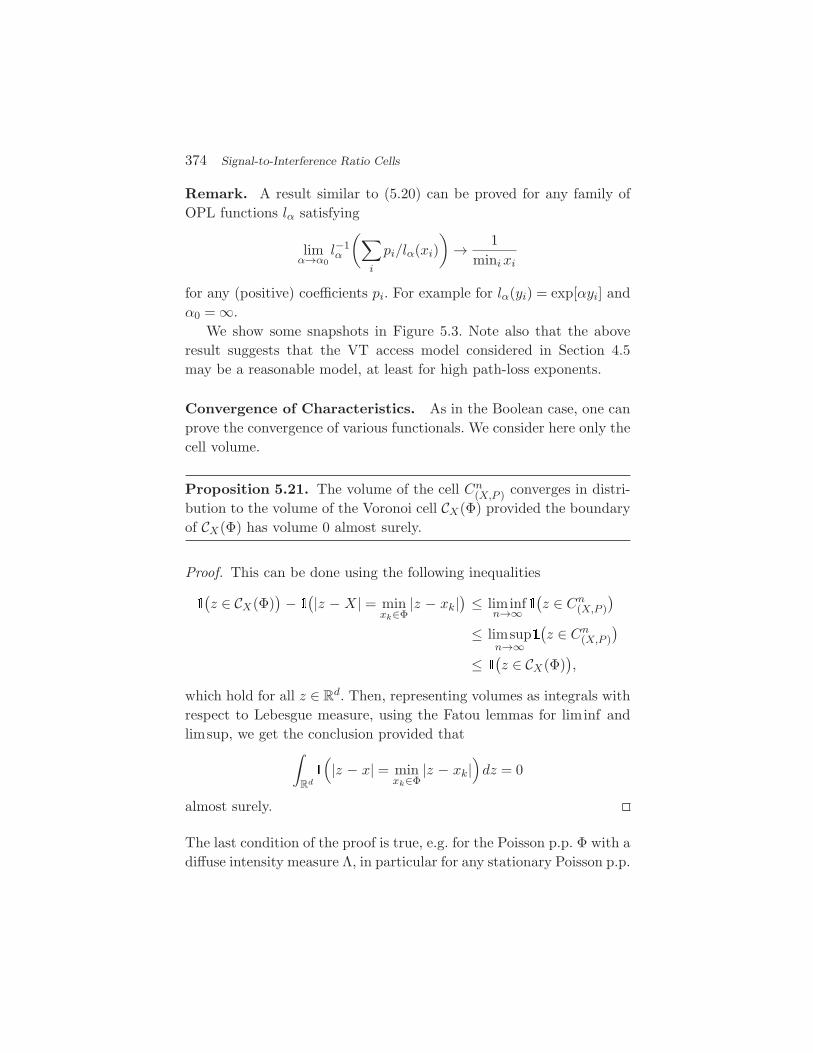
374 Signal-to-Interference Ratio Cells
Remark. A result similar to (5.20) can be proved for any family ofOPL functions lα satisfying
limα→α0
l−1α
(∑i
pi/lα(xi))
→ 1mini xi
for any (positive) coefficients pi. For example for lα(yi) = exp[αyi] andα0 = ∞.
We show some snapshots in Figure 5.3. Note also that the aboveresult suggests that the VT access model considered in Section 4.5may be a reasonable model, at least for high path-loss exponents.
Convergence of Characteristics. As in the Boolean case, one canprove the convergence of various functionals. We consider here only thecell volume.
Proposition 5.21. The volume of the cell Cn(X,P ) converges in distri-
bution to the volume of the Voronoi cell CX(Φ) provided the boundaryof CX(Φ) has volume 0 almost surely.
Proof. This can be done using the following inequalities(z ∈ CX(Φ)
) − (|z − X| = minxk∈Φ
|z − xk|) ≤ liminf
n→∞(z ∈ Cn
(X,P ))
≤ limsupn→∞
(z ∈ Cn
(X,P ))
≤ (z ∈ CX(Φ)
),
which hold for all z ∈ Rd. Then, representing volumes as integrals with
respect to Lebesgue measure, using the Fatou lemmas for liminf andlimsup, we get the conclusion provided that∫
Rd
(|z − x| = min
xk∈Φ|z − xk|
)dz = 0
almost surely.
The last condition of the proof is true, e.g. for the Poisson p.p. Φ with adiffuse intensity measure Λ, in particular for any stationary Poisson p.p.
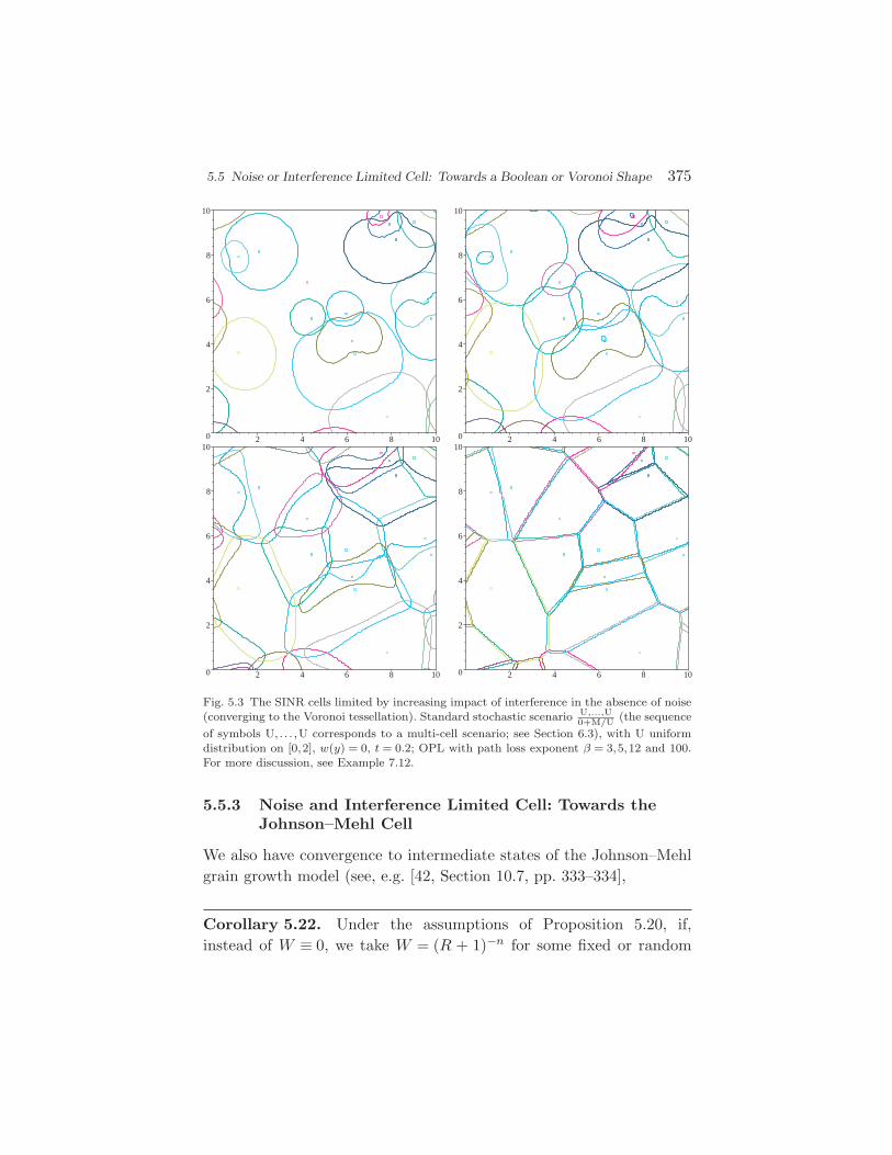
5.5 Noise or Interference Limited Cell: Towards a Boolean or Voronoi Shape 375
0
2
4
6
8
10
2 4 6 8 10 0
2
4
6
8
10
2 4 6 8 10
0
2
4
6
8
10
2 4 6 8 10 0
2
4
6
8
10
2 4 6 8 10
Fig. 5.3 The SINR cells limited by increasing impact of interference in the absence of noise(converging to the Voronoi tessellation). Standard stochastic scenario U,...,U
0+M/U (the sequenceof symbols U, . . . ,U corresponds to a multi-cell scenario; see Section 6.3), with U uniformdistribution on [0,2], w(y) = 0, t = 0.2; OPL with path loss exponent β = 3,5,12 and 100.For more discussion, see Example 7.12.
5.5.3 Noise and Interference Limited Cell: Towards theJohnson–Mehl Cell
We also have convergence to intermediate states of the Johnson–Mehlgrain growth model (see, e.g. [42, Section 10.7, pp. 333–334],
Corollary 5.22. Under the assumptions of Proposition 5.20, if,instead of W ≡ 0, we take W = (R + 1)−n for some fixed or random
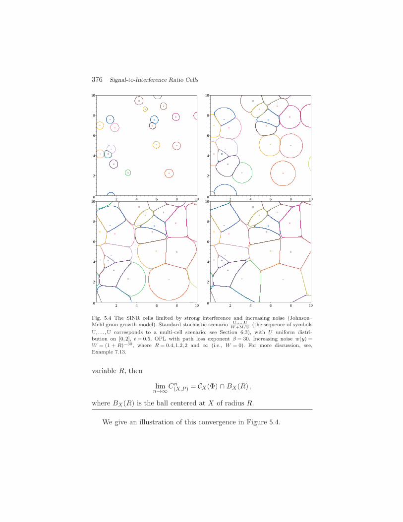
376 Signal-to-Interference Ratio Cells
0
2
4
6
8
10
2 4 6 8 10 0
2
4
6
8
10
2 4 6 8 10
0
2
4
6
8
10
2 4 6 8 100
2
4
6
8
10
2 4 6 8 10
Fig. 5.4 The SINR cells limited by strong interference and increasing noise (Johnson–Mehl grain growth model). Standard stochastic scenario U,...,U
W+M/U (the sequence of symbolsU, . . . ,U corresponds to a multi-cell scenario; see Section 6.3), with U uniform distri-bution on [0,2], t = 0.5, OPL with path loss exponent β = 30. Increasing noise w(y) =W = (1 + R)−30, where R = 0.4,1.2,2 and ∞ (i.e., W = 0). For more discussion, see,Example 7.13.
variable R, then
limn→∞Cn
(X,P ) = CX(Φ) ∩ BX(R) ,
where BX(R) is the ball centered at X of radius R.
We give an illustration of this convergence in Figure 5.4.
6Interacting Signal-to-Interference Ratio Cells
6.1 Introduction
We consider now the relationships between several SINR cells. As inChapter 5, let Φ =
∑i ε(xi,mi) be an i.m.p.p. with points xi in R
d
and marks mi in R. Let IΦ(y) be a scalar shot-noise field on R
d
generated by Φ and the response function L:Rd × Rd × R
→ R+.
Definition 6.1. Let n be a positive integer and let (Xi,Mi), i =1, . . . ,n, X ∈ R
d, M ∈ R, be a collection of n marked points. Let ti ≥ 0,
i = 1, . . . ,n be a collection of n thresholds. We define the SINR cells ofthis collection of marked points and thresholds in the shot-noise fieldIΦ and the thermal noise field w(y) ≥ 0 as
C(Xi,Mi) = C(Xi,Mi)(Φ,(Xj ,Mj), j = i,w,ti)
=
y : L(y,Xi,m) ≥ ti(IΦ(y) + κ∑j =i
L(y,Xj ,Mj) + w(y))
,
(6.1)
where 0 < κ ≤ 1 is some constant.
377

378 Interacting Signal-to-Interference Ratio Cells
If κ = 1, this is the collection of SINR cells of the points Xi, i =1, . . . ,n for the SN created by the p.p.
Φ +n∑
i=1
δXi,Mi .
If κ = 1, the response of the points Xj and that of the points of Φ areweighted differently.
Example 6.1 (Downlink in a Code Division Multiple Accesscell with several users). Let Φ be an i.m. Poisson p.p. representingthe location of base stations using Code Division Multiple Access(CDMA) (see Section 25.1.4 in Volume II). Let X be the location ofa tagged base station with n users. Since all n users are served by thetagged base station, we take Xi = X for i = 1, . . . ,n. In this case thecell C(Xi,Pi) gives the locations where user i, when served by the taggedbase station with power Pi, receives a signal strong enough to sustainthe goodput that corresponds to the SINR threshold ti. In this casethe factor κ might stem from the fact that orthogonal signatures areused within a cell. Another essential feature of CDMA is power control(addressed in Section 25.2 in Volume II).
Remark 6.1. Note that when changing the thresholds ti to
t′i =ti
1 + κti(6.2)
one can replace∑
j =i L(y,Xj ,Mj) in (6.1) by∑n
j=1 L(y,Xj ,Mj).Indeed,
L(y,Xi,m) ≥ ti(IΦ(y) + κ∑j =i
L(y,Xj ,Mj) + w(y))
iff
L(y,Xi,m) ≥ ti/(1 + κti)(IΦ(y) + κ
n∑j=1
L(y,Xj ,Mj) + w(y)).
This means that
C(Xi,Mi)(Φ,(Xj ,Mj)j =i, ti)=C(Xi,Mi)(Φ,(Xj ,Mj)j=1,...,n, t′i).
6.2 Constraints on Cell Intersections 379
6.2 Constraints on Cell Intersections
We now comment on a basic algebraic property which sheds some lighton the fact that the SINR cells are typically deformed and may haveholes, and this happens even in the case of a simple isotropic responsefunction L.
Proposition 6.2. Consider the collection of SINR cells C(Xi,Mi) =C(Xi,Mi)(Φ,(Xj ,Mj), j = i, ti) of Definition 6.1. For any subset J ⊂1, . . . ,n of cells, if
⋂i∈J C(Xi,Mi) = ∅, then
∑i∈J t′i ≤ 1/κ, where t′i is
given by (6.2).
Proof. Assume y ∈⋂i∈J C(Xi,Mi) = ∅. Then by Remark 6.1, we havethe set of inequalities
L(y,Xi,m) ≥ t′iκ∑j∈J
L(y,Xj ,Mj), i ∈ J ,
Summing them up, we obtain∑j∈J
L(y,Xj ,Mj) ≥ κ∑i∈J
t′i∑j∈J
L(y,Xj ,Mj) ,
which is equivalent to∑
i∈J t′i ≤ 1/κ.
Remark 6.2. Note that the above result is purely algebraic (nostochastic assumptions are made). It says that by increasing the sig-nals L(y,Xi,Mi) that one cannot cover a given point y by arbitrarilymany cells. In particular, in the case of constant ti = t no location canbe covered by more than s = tκ/(1 + tκ), cells, whatever the loca-tions Xi of the transmitters and whatever the strength of their signalsL(y,Xi,Mi). For example, in Figure 5.3 s = 4, while in Figure 5.4 s = 1inhibits any overlapping of cells.
Example 6.3 (Pole capacity of the downlink CDMA cell). Letus continue Example 6.1 and consider one given antenna, say locatedat X, which transmits a compound signal of total power P1 + · · · + Pn
for serving n users with respective bit-rates corresponding to tk,
380 Interacting Signal-to-Interference Ratio Cells
k = 1, . . . ,n. Since the possible locations of these users are describedby the cells C(X,Pk), by Proposition 6.2, if
∑ni=1 t′i > 1/κ then these
cells cannot simultaneously cover any given location. This means thatif all the users are at the same location, they cannot be served simul-taneously by the tagged base station, no matter how strong the emit-ted powers are. If one assumes ti = t, this mean that no more thann1 ≤ (1 + κt)/(κt) users can be served. This upper bound for the num-ber of users is called the pole capacity of the CDMA cell. It gives themaximal number of users that can be served at a given location witha bit-rate corresponding to the SINR threshold t.
6.3 Stochastic Scenarios and Coverage Probabilities
By the standard stochastic scenario for collections of SINR cells, weunderstand the framework described in Section 5.3, with the responsefunction L(y,x,p) = p/l(|y − x|), where l is an omni-directional powerattenuation function (see Section 23.1.2 in Volume II), with assump-tion (3) of the single cell scenario replaced by:
(3∗) The marks Mj = Pj of the points Xj (j = 1, . . . ,n) generatingthe cells C(Xj ,Pj) are mutually independent, independent ofΦ, and have the same distribution function G as the marksof Φ.
In a slightly more general case one can consider the scenario where
(3∗′) The marks P1, . . . ,Pn are mutually independent and indepen-
dent of Φ and have some given distribution G′.
Kendall-like Notation cont. Extending our previous notation forSINR, we call the above framework for collections of SINR cells
GI,...,GIW+GI/GI model, where GI’s in the numerator denote the general dis-tribution of the Pj ’s.
6.4 Joint Point-Coverage Probability
Assume the standard scenario for collections of SINR cells. Lety1, . . . ,yn be n locations. We are interested in theprobability that for

6.4 Joint Point-Coverage Probability 381
all j = 1, . . . ,n the cell C(Xj ,Pj) covers location yj :
pX1,...,Xn(y1, . . . ,yn)
= P
n⋂
j=1
yj ∈ C(Xj ,Pj)(Φ,(Xl,Pl), l = j,W,ti)
= P
n⋂
j=1
Pj ≥ til(|yj −Xj |)
(IΦ(yj)+κ
∑l =i
Pl/l(|yj −Xl|)+W)
.
(6.3)
Special cases are the probability pX1,...,Xn(y, . . . ,y) that all cells cover agiven point y and the probability pX,...,X(y1, . . . ,yn) that a given nodeusing n independent powers, covers n different locations (cf. Exam-ple 6.3). Recall, that in all these cases, the powers Pl for l = j areconsidered as interference with respect to the transmission j.
The following result gives the joint point-coverage probability forthe M,...,M
W+GI/GI model, where the received powers P1, . . . ,Pn are exponen-tial with mean 1/µ. Recall from Section 5.4 that this might correspondto a situation when Pj = Pf j , where P is some constant emitted powerand f j is an exponential random variable modeling Rayleigh fading inthe channel from Xj to yj . For simplicity we state and prove the resultfor two cells.
Let ljk = l(|yk − Xj |), k,j = 1,2 and let L(I1,I2)(s1,s2) be the jointLaplace transform of the vector (IΦ(y1), IΦ(y2)) and LW (s) the Laplacetransform of W .
Proposition 6.4. Consider the standard M,Mw + GI/GI model. If
δ =t1t2κ
2l11l22
l21l12< 1 (6.4)
then the joint point-coverage probability is equal to
pX1,X2(y1,y2) = µ1 − δ
(l21 + t1l11κ)(l12 + t2l22κ)
×LW
(ξ1 + ξ2
1 − δ
)L(I1,I2)
( ξ1
1 − δ,
ξ2
1 − δ
),
where ξi=tiliilji(lij+tjljjκ), i, j=1,2, i=j. Otherwise pX1,X2(y1,y2)=0.
382 Interacting Signal-to-Interference Ratio Cells
Proof. Note first that the condition (6.4) is necessary for the inequal-ities in (6.3) with j = 1,2 and n = 2 to hold when W ≡ 0 and IΦ ≡ 0.So it is necessary for pX1,X2(y1,y2) > 0. In what follows, we assume itis satisfied. Similarly as in the proof of Proposition 5.9 we have
pX1,X2(y1,y2) =∫ ∞
0
∫ ∞
0
∫ ∞
0A(u,v1,v2)
×P(W = du,I1 = dv1, I2 = dv2
),
with
A(v,u1,u2) =∫ ∞
0
∫ ∞
0
(p1 ≥ t1l11(u + v1 + κp2/l21)
)× (
p2 ≥ t2l22(u + v2 + κp1/l12))µ2e−µ(p1+p2) dp1dp2.
For ai, bi ≥ 0, i = 1,2 and b1b2 < 1, we have∫ ∞
0
∫ ∞
0(p1 ≥ a1 + b1p2) (p2 ≥ a2 + b2p1)µ2e−µ(p1+p2) dp1dp2
= µ1 − b1b2
(1 + b1)(1 + b2)exp(
−µa1(1 + b2) + a2(1 + b1)
1 − b1b2
).
Taking ai = tilii(u + vi), bi = tiliiκ/lji with i, j = 1,2, j = i, we observethat b1b2 < 1 is equivalent to (6.4) which we assume to be satisfied.Thus we have
pX1,X2(y1,y2) =1 − δ
(l21 + t1l11κ)(l12 + t2l22κ)
×∫ ∞
0
∫ ∞
0
∫ ∞
0e−µ((v+u1)ξ1+(v+u2)ξ2)/(1−δ)
×P(W = du,I1 = dv1, I2 = dv2
),
and the result follows.

7Signal-to-Interference Ratio Coverage
7.1 Introduction
Let Φ =∑
i ε(xi,mi,ti) be a marked point process, with points xi in Rd
and marks mi in R (as in Chapter 5) and ti ∈ R
+. As in Chapter 5,let IΦ(y) be the SN on R
d, generated by Φ =∑
i ε(xi,mi) (i.e., Φ withoutthe marks ti) and by the response function L:Rd × R
d × R → R
+.
Definition 7.1. We define the SINR coverage process generated by Φand the thermal noise field w(y) ≥ 0, as the following union of SINRcells:
ΞSINR = Ξ(Φ,w)
=⋃
(xi,mi,ti)∈Φ
C(xi,mi)(Φ − ε(xi,mi),w,ti)
=y : there exist (xi,mi, ti) ∈ Φ : L(y,xi,mi)
≥ ti(IΦ(y) − L(y,xi,mi) + w(y)). (7.1)
383

384 Signal-to-Interference Ratio Coverage
Remark. From Remark 6.1, C(xi,mi)(Φ − ε(xi,mi),w,ti) in (7.1) isequal to C(xi,mi)(Φ,w,t′i) with
t′i =ti
1 + ti. (7.2)
Moreover, if t′i > 0 for all i, then ΞSINR can also be expressed as
ΞSINR = y:XΦ(y) ≥ IΦ(y) + w(y) ,
where
XΦ(y) = max(xi,mi,ti)∈Φ
(L(y,xi,mi)
ti
)is a max-shot-noise process generated by Φ and the response functionL(y,x,m,t) = L(y,x,m)/t (cf. Section 2.4), provided the max is welldefined, for example when there is an a.s. finite number of cells coveringpoint y.
Standard Stochastic Scenario and Kendall-like Notation. Weshall often consider the following standard scenario for the coverageprocess.
(1) We assume that Φ is a general stationary independentlymarked point process with points in R
2 and intensity λ > 0.(2) The marks (mi = (pi, ti)) have some given distribution
Pp ≤ u,t ≤ v = G(u,v) that does not depend on the loca-tion of the corresponding point.
(3) The thermal noise field w(y) = W is constant in space andequal everywhere to some non-negative random variableW ≥ 0 independent of Φ.
Note that assumptions (1) and (2) correspond to some natural exten-sion (marks ti are added) of the standard scenario for SN, for whichthe following isotropic response function L(y,x,p) = p/l(|y − x|) isassumed, with l some omni-directional power attenuation function (seeSection 23.1.2 in Volume II).
Extending our previous Kendall-like notation to SINR coverage, wecall the above scenario the GI/GI
W+GI/GI model.

7.2 Typical Cell of the Coverage Process 385
Fig. 7.1 SINR coverage model without fading.
Figure 7.1 shows a realization of the SINR coverage model M/DW+M/D
while Figure 7.2 shows the same situation with an independent fadingfor each point.
7.2 Typical Cell of the Coverage Process
Let P !(x,m,t) denote the reduced Palm distribution of Φ (see Section 1.4).
Recall that one can consider this distribution as the conditional distri-bution of Φ − ε(x,m,t) given that Φ((x,m,t)) > 0. Under P !
(x,m,t), the
SINR cell C(x,m,t)(Φ,w,t) is called the typical cell of the coverage processΞSINR at (x,m,t).1
From Corollary 2.2, in the case of an i.m.p.p., P !(x,m,t) is also the dis-
tribution of an independently marked point process with marks havingthe original distribution.
1 The name “typical cell” is natural in the stationary case.

386 Signal-to-Interference Ratio Coverage
Fig. 7.2 SINR coverage model with point dependent fading.
If moreover Φ is an i.m. Poisson p.p. then by Slivnyak’s Theorem(see Theorem 1.13) the reduced Palm distribution P !
(x,m,t) is equal to
the original Poisson distribution of Φ. Moreover, the moment measureM of Φ is equal to
M(d(x,m,t)) = F (d(m,t))Λ(dx),
where Λ is the intensity measure of the Poisson p.p. Φ. This allows usto interpret many results obtained in Chapter 5 for a single SINR cellas concerning the typical cell of the SINR coverage process ΞSINR with(possibly) a randomized mark P . Note also that Assumption (3) of thestandard scenario for SINR cells states that P is randomized accordingto its original generic distribution.
7.3 Nearest Transmitter Cell
Consider a GI/GIW+GI/GI model. We are interested in the probability that a
given location, say the origin y = 0, is covered by the cell of the nearest

7.3 Nearest Transmitter Cell 387
transmitter:
p∗ = P
y ∈ C(xo,po)(Φ − ε(xo,po),W,t)
= P
po ≥ l(|xo|)t(W + IΦ(y) − po/l(|xo|)),where xo = arg minxi∈Φ |xi| (by Lemma 4.2, xo is almost surely welldefined) and po is the mark of x∗ in Φ. In the case of Poisson p.p.,the joint distribution of (x∗,p∗) and Φ − ε(xo,po) is known. Thus, con-ditioning on x∗, one can evaluate p∗ by similar arguments as p0(y) (seeSection 5.3.1). These calculations are explicit in the M/M
W+M/M model.
Proposition 7.1. For the M/MW+M/M model with deterministic ti = t
p∗ =∫ ∞
02πλr exp(−λπr2)LW (µtl(r))
×exp(
−2πλ
∫ ∞
r
u
1 + l(u)/(tl(r))du
)dr , (7.3)
where E[po] = 1/µ.
Proof. Recall that P|xo| > r = e−λπr2. Moreover, given xo = r, Φ −
ε(xo,po) is an i.m. Poisson p.p. with intensity λ (|x| > r) and indepen-dent of p∗. Thus conditioning on |xo| = r, by the same arguments as inthe proof of Proposition 5.5, the coverage probability is equal to
LW (µtl(r))exp(
−2πλ
∫ ∞
r
u
1 + l(u)/(tl(r))du
). (7.4)
We obtain the result by integrating with respect to the law of |xo|.
Example 7.2. Consider OPL 3 with β = 4 and W ≡ 0. Then usingthe fact that∫ ∞
r
u
1 + l(u)/(tl(r))du =
r2
4
√t(π − 2arctan(1/
√t)),
we get that
p∗ =∫ ∞
02πλr exp
(−r2λπ
(1 +
12
√t(π − 2arctan(1/
√t))))
dr.
(7.5)
388 Signal-to-Interference Ratio Coverage
7.4 ΞSINR as a Random Closed Set
We now consider some stochastic-geometry theoretic properties ofSINR coverage processes. We require that the typical cell be a closed setfor M(d(x,m,t)) almost all (x,m,t) ∈ R
d × R × R
+. By Campbell’sformula, one can then conclude that under the original (unconditional)distribution of ΞSINR, all the cells C(xi,mi)(Φ − ε(xi,mi),w,ti) are almostsurely closed sets. In the case of an i.m.p.p., conditions for the typicalcell to be a closed set can hence be found in Corollary 5.2.
In stochastic geometry it is customary to require ΞSINR to be aclosed set (note that the countable union of closed sets need not beclosed). In fact, we require the stronger property that for any givenbounded set in R
d (with compact closure), the number of cells thathave non-empty intersection with it is almost surely finite.2
Denote by NK the random number of cells
Ci = C(xi,mi)(Φ − ε(xi,mi),w,ti) (7.6)
that hit a given bounded set K
NK =∑
i
(K ∩ Ci = ∅). (7.7)
In what follows, we assume that Φ is an i.m. Poisson p.p. and we giveseveral instances of moment-conditions (bearing on the distributionF (d(m,t)) of the generic mark (m,t) and the intensity measure Λ ofthe p.p.) for E[NK ] to be finite for arbitrary large K. Later on we willcomment on the general stationary case as well.
Note first that the required property is always satisfied if Λ(Rd) < ∞(i.e. when Φ has almost surely a finite number of points in R
d). In thefollowing, we will assume one of the two following conditions on the
2 An equivalent statement is that the collection of cells is a.s. a Radon point measure onthe space of closed sets, so that it can be treated as a point process
∑(xi,mi,ti)
εCi
on the space of closed sets. This is a typical assumption for coverage processes (in particularfor the Boolean model, see e.g. [42], Equation (3.1.1), p. 59).

7.4 ΞSINR as a Random Closed Set 389
response function:
(A1) There exists a finite real number R∗, such that L(y,x,m) = 0for all m ∈ R
and y,x ∈ Rd with |y − x| > R∗.
(A2) There exist positive constants A and β such that L(y,x,m) ≤A|s| |z|−β, for all y,x ∈ R
d,s ∈ R, where | · | denotes the
Euclidean norm.
Note that condition (A2) is satisfied for the standard scenario withOPL 1 and OPL 2.
Proposition 7.3. Let Φ an be i.m. Poisson p.p. with intensity Λ.Assume that ti > 0 a.s. We have
E[NK ] < ∞ (7.8)
for an arbitrary large K if one of the following conditions holds:
(i) Condition (A1) is satisfied and w(x) > 0 for all x ∈ Rd with
probability 1,(ii) Condition (A2) is satisfied, w(t) ≥ W > 0 a.s. for some (pos-
sibly random) variable W , and for all R > 0
E
[Λ
(B
(0,R +
(A|m0|t0W
)1/β))]< ∞ . (7.9)
(iii) Condition (A2) is satisfied, L(y,x,m) > 0 a.s. for all y ∈ Rd,
and for all R > 0∫Rd
e−Λ(B(0,|x|))E
[Λ
(B
(0,R +
(A|m1|
t1L(R,x,m0)
)1/β))]×Λ(dx) < ∞, (7.10)
where m0 is independent of (m1, t1), with both havingthe distribution of the marginals of a typical mark, andL(r,x,m) = infy:|y|≤r L(y,x,m).
390 Signal-to-Interference Ratio Coverage
Proof. In order to prove (7.8), we construct various Boolean modelsdominating our coverage process ΞSINR and we use Lemma 3.1 to ensurethat the number of cells of the Boolean model which intersect K is offinite mean, which is equivalent to
E[Λ(Ξ ⊕ K)] < ∞ , (7.11)
where Ξ is the generic grain of the BM.
(i) Under (A1), we have Ci ⊂ B(Xi,R∗) and the result follows
from the fact that (7.11) is obviously finite for the Booleanmodel with deterministic cells.
(ii) Under (A2) we have
Ci =
y:L(y,xi,mi) ≥ ti(IΦ(y) − L(y,xi,mi) + w(y))
⊂
y:L(y,xi,mi) ≥ tiW
⊂
y:A|mi| |y − xi|−β ≥ tiW
⊂
y: |y − xi| ≤(
A|mi|tiW
)1/β. (7.12)
Thus, we have Ci ⊂ B(xi,ρi) , a.s., where
ρi =(
A|mi|tiW
)1/β
.
There is no loss of generality in assuming that the boundedset K is the ball B(0,R) and the result now follows from thesimple observation that B(0,R) ⊕ B(0,ρi) = B(0,R + ρi).
(iii) Now we do not assume anything about w(t) (thus it mayby positive or null). Instead we use one of the points of theprocess Φ to guarantee a sufficient level for the variable IΦand thus bound cell sizes from above. Let x0 denote the pointof Φ which is nearest to the origin, and let m0 be its mark.
7.4 ΞSINR as a Random Closed Set 391
We have
NK = (K ∩ C0 = ∅) +∑i =0
(K ∩ Ci = ∅)
≤ 1 +∑i =0
(K ∩ Ci = ∅) . (7.13)
For any point xi = x0 (i.e., |xi| > |x0|) of the point process,with mark mi, ti, and K = B(0,R)
Ci(Φ) ∩ K ⊂
y: |y| ≤ R and |y − xi| ≤(
A|mi|tiL(y,x0,m0)
)1/β
⊂
y: |y − xi| ≤(
A|mi|ti infy, |y|≤R L(y,x0,m0)
)1/β⊂ B
(xi,ρ(R,mi, ti,x0,m0)
),
where
ρ(R,mi, ti,x0,m0) =(
A|mi|tiL(R,x0,m0)
)1/β
.
Using now (7.13) and the assumption that x0 is the pointnearest to the origin, we get
E[NK ] ≤ E[1 +
∑i =0
(K ∩ Ci = ∅)]
= E
[∫Rd
(Φ(Bo(0,x0)) = 0
)×(
1 +∑i =0
(K ∩ Ci = ∅))
Φ(dx0)]
≤∫
Rd
e−Λ(B(0,|x0|))
×E
[1+
∑i, |xi|>x0
(K ∩ B(xi,ρ(R,mi, ti,x0,m0)) =∅)
]Λ(dx0) .

392 Signal-to-Interference Ratio Coverage
So by (7.11) for the Boolean model with Gi = B(0,ρ(R,mi, ti,
x0,m0)) conditioned on x0,m0
E[NK ] ≤∫
Rd
e−Λ(B(0,|x0|))
×E[1 + Λ
(K ⊕ B
(0,ρ(R,m1, t1,x0,m0)
))]Λ(dx) .
The proof is concluded by observing that B(0,R) ⊕B(0,ρ(· · ·)) = B(0,R + ρ(· · ·)).
Corollary 7.4. Let Φ be an independently marked and homogeneousPoisson p.p. with intensity Λ(dx) = λdx. Then (7.9) is equivalent tothe following condition
E[( |m0|
t0W
)d/β]< ∞, (7.14)
whereas (7.10) is equivalent to the conjunction of the following twoconditions∫
Rd
e−λνd|x|d(E[L(R,x,m0)]
)−d/βdx < ∞, E
[( |m0|t0
)d/β]< ∞.
(7.15)
Remark. Conditions analogous to parts (i) and (ii) of Proposition 7.3can be observed in the stationary ergodic case; (7.9) and (7.14) have thesame form with E[. . .] replaced with E0[. . .], where E0 is the expectationw.r.t. the Palm distribution of the mark (m0, t0). The proof is basedon Campbell’s formula. Part (iii) has no generalization due to the lackof an explicit form of the joint distribution of x0 (the point which isnearest to the origin) and the remaining part of a general point process.
7.5 The Coverage Process Characteristics
Our goal in this section is to analyze the coverage process ΞSINR, andmore specifically, the distribution of the number of cells covering agiven point. From this, the volume fraction and other characteristicsof ΞSINR can be derived. Let Nx = Nx (cf. (7.7)) denote the number

7.5 The Coverage Process Characteristics 393
of cells covering a given point x. For all integers k, let k(n) = k(k −1) . . .(k − n + 1)+, where k+ = max(0,k). Below, we give formulae forfactorial moments E[N (n)
x ] of Nx. From this, the distribution of Nx canbe derived using the formula
P(Nx = n) =1n!
∞∑k=0
(−1)k E[N (n+k)x ]k!
, (7.16)
which follows from the well-known expansion of the generating function.Of course, these expansions usually require strong conditions (existenceof all moments and convergence of the series). However, these issuesdisappear when Nx is bounded.
7.5.1 Bounded Nx
Suppose now that the distribution of the marks is such that ti arebounded away from 0, i.e.
(B) ti ≥ ρ a.s. for some constant ρ > 0.
Using the result of Proposition 6.2, we immediately have the followingproperty of the coverage process:
Corollary 7.5. If Condition (B) is satisfied then Nx < 1/ρ almostsurely.
Proof. Assume that n = Nx cells cover point x. Then from Proposi-tion 6.2,
∑nk=1 tik ≤ 1, where tik , k = 1, . . .n are marks of the cells cov-
ering x. Since tik ≥ ρ, so n ≤ 1/ρ.
Remark. This bound suggests an analogy with queueing theory. Onecan think of queueing theory as a way of sharing time between cus-tomers arriving at a queue according to some point process on the line,and requiring some given service times. We can also think of our cov-erage process as a way of sharing space between the points of a spatialpoint process with given marks. Under the condition mentioned in thelast lemma, the coverage process can be seen as a spatial analogue of
394 Signal-to-Interference Ratio Coverage
the -server queue, with = minn integer : n ≥ 1/ρ, in that no pointin space can be covered by more than cells; in the same way, the -server queue forbids that at any point in time, more than -customerscould be served. Note that sharing actually means quite different thingshere and there: in queues, the sharing of time is implemented by shift-ing customers in excess to later times, while keeping their service timesunchanged. In contrast, for this coverage process, sharing of space isobtained by shrinking the marks: if one defines the space request of pointx0 as the set C
(0)0 = y:L(y,x0,m0) ≥ t0w(y), which would be the
share of space obtained by x0 if there were no other points, then one cansee the set C0 =
y:L(y,x0,m0) ≥ t0(IΦ(y) − L(y,x0,m0) + w(y))
, as
a shrunken version of C(0)0 resulting from the competition with the other
points.In the same vein, the Boolean model, which is a limiting case of
our coverage process (see Section 5.5.1), can also be seen as a spatialanalogue of the infinite server queue, and that in this case, the analogyis quite strong, with in particular the same Poisson distribution for thenumber of marks (customers or cells) covering a given (time or space)point.
7.5.2 Factorial Moments of Nx
We are now in a position to prove the following result.
Proposition 7.6. Assume Φ is a simple i.m. Poisson p.p. with inten-sity measure Λ. Then the nth factorial moment of the number Nx ofcells of ΞSINR(Φ) covering point x is equal to
E[N (n)x ] =
∫(Rd)n
P(
x ∈n⋂
k=1
C(xk,mk)
(Φ +
n∑i=1,i =k
ε(xi,mi),w(y), ti))
Λ(dx1) · · ·Λ(dxn), (7.17)
where Φ is distributed as Φ without marks ti and (mi, ti)ni=1 are mutu-
ally independent vectors, independent of Φ distributed as its genericmark. This relation holds provided the integral on the right hand sideis finite. In particular, if Φ is a homogeneous Poisson p.p. with intensity
7.5 The Coverage Process Characteristics 395
Λ(dx) = λdx then for each x ∈ Rd
E[Nx] = λE[∣∣C(x,m0)(Φ,w(y), t0)
∣∣] , (7.18)
where |C| is the d-dimensional volume of the cell C.
Proof. For a particular realization Φ of the marked Poisson p.p, denoteby Φ(n) its nth factorial power, that is the following point measure on(R
d × R × R
+)n
Φ(n) =∑
xi1 ,...,xin∈Φdistinct
ε((xi1 ,...,xin ),(mi1 ,...,min ),(ti1 ,...,tin )) .
In other words, Φ(n) consists of all n-tuples of distinct points of Φ (seeChapter 9). Now we can write the factorial power (Nx)(n) of the numbercells covering point x as the following integral with respect to Φ(n)
N (n)x =
∫(Rd)n
n∏k=1
(x ∈ C(xk,mk)(Φ,w(y), ti)
)×Φ(n)(d((x1, . . . ,xn),(m1, . . . ,mn),(t1, . . . , tn)
). (7.19)
We get (7.17) by applying the refined Campbell theorem to the (seeCorollary 9.2) expectation of this integral and the fact that facto-rial moment measures of Poisson processes are Lebesgue measures(Proposition 9.1).
Remark. For the finiteness of the integral that appears in Proposi-tion 7.6, it is enough to assume exactly the same conditions as for theσ-finiteness of the mean measure of
∑i εCi given in Proposition 7.3
parts (i) and (ii). In the case P(w(y) = 0) > 0, however, some integralsof the negative moments of order nd/α of L(y,x0,m) have to be finite,where x0 is the point which is nearest to the origin. Details can befound in [1].
7.5.3 Volume Fraction
The volume fraction p = P(0 ∈ ΞSINR) is a basic characteristic of astationary coverage process. Strictly speaking, it can be defined andcalculated for any coverage process, but then the notion might be

396 Signal-to-Interference Ratio Coverage
misleading, since it is only when we assume that the probabilityP(x ∈ ΞSINR) does not depend on x, that we can say that the expectedfraction of the d-dimensional volume of ΞSINR per unit ball is equalto p (cf. the remark after Definition 3.4). Thus for the remaining partof this section, we assume that Φ is a homogeneous Poisson p.p. withintensity λ, that the function L(y,x,m) = L(y − x,0,m) depends onlyon (|x − y|,m)) and that w(y) is stationary. Using the expansion (7.16)we can write p =
∑∞k=1(−1)k+1/k!E[(N0)(k)], where the coefficients are
given in Proposition 7.6, provided all moments are finite and the seriesis convergent. Note however, that if we assume condition (B) of Sec-tion 7.5.1 (ti ≥ ρ > 0 a.s.), then the expansion has only finitely manynon-zero terms.
Note that the dependent marking of our coverage process (cellsare dependent) makes it impossible to calculate the volume fractionin the way typically used for Boolean models. Nevertheless using thefactorial moment expansion technique for a general class of functionalsof spatial p.p.s presented in [4] (see also references therein), the firstorder approximation of the volume fraction can be represented as
p = λ
∫Rd
p0(x)dx + O(λ2) = λE[ |C(0,M)| ] + O(λ2) , (7.20)
where p0(x) is the single (typical) cell coverage probability andE[ |C(0,M)| ] is the expected volume of the typical cell. The first termin the last formula differs from the formula (7.18) for E[N0] only inthat Φ is replaced by the null measure (without points). More generalapproximation formulae (involving polynomials in λ) can be obtainedvia this expansion technique.
7.5.4 Noise or Interference Limited Coverage — ExtremalCases
The aim of this section is to extend the results of Section 5.5 on theconvergence of cells Ci towards, e.g. those of the BM or those of a VTto the convergence of the whole SINR coverage process.
Noise Limited Cells — Towards a Boolean Model. By analogyto what was done in Section 5.5.1 consider the following family of SINR
7.5 The Coverage Process Characteristics 397
coverage processes
Ξ(κ)SINR =
⋃i
C(κ)i ,
where
C(κ)i = y:L(y,xi,mi) ≥ t(κ(IΦ(y) − L(y,xi,m)) + W ).
Note that (for simplicity) we have assumed a random noise W whichis constant in space, but possibly random.
Proposition 7.7. Assume that the conditions of Corollary 5.2 withw(y) = W are satisfied as well as Condition (1) in Section 5.5.1.Then, almost surely on the space of closed sets, limκ→0 Ξ(κ)
SINR = Ξ(0)SINR
(Painleve–Kuratowski convergence), provided Ξ(κ)SINR is a random closed
set for κ ∈ [0,κ0] and some κ0 > 0.
Proof. Observe that⋃κ
Ξ(κ) =⋃κ
⋃i
C(κ)i =
⋃i
⋃κ
C(κ)i =
⋃i
C(0)i =
⋃i
C(0)i ,
where the last but one equality follows from (5.9) and the last one fromthe assumption that Ξ(0)
SINR is a closed set.
Remark. Suppose that Φ is an independently marked Poisson pointprocess. Then Ξ(0)
SINR given W is a Boolean model with grains C(0)i =
y : L(y,xi,mi) ≥ tiW.
Example 7.8. We now illustrate Proposition 7.7 by showing somepatterns of our coverage process ΞSINR “conforming” to a Booleanmodel pattern. We simulated a Poisson p.p. with 60 points on thesquare [−5,15]2 (so that λ = 0.15). While observing only the square[0,10]2, we take all 60 points of the larger square into account for eval-uating IΦ. We assume the standard scenario for the coverage processwith the OPL function (1 + |y|)3. The pi’s are uniformly distributed

398 Signal-to-Interference Ratio Coverage
on [0,2], ti ≡ 1 and W ≡ 0.1. The various patterns result from tak-ing various values for κ. Figure 5.2 presents the coverage processΞSINR “on its way” to a Boolean model. We have: (a) κ = 0.4; notethat 2κ < 1 < 3κ; thus at most two cells could cover any given point,although this is not observed; (b) κ = 0.2; since 4κ < 1 = 5κ, at mostfour cells could cover any given point; (c) κ = 0.1; cells occupy moreand more of the final space that they occupy under the Boolean modelregime; (d) κ = 0.0001; almost the limiting case where each cell is adisc with independent radius distributed as (10p)1/3 − 1 (with mean201/3 × 3/4 − 1 ≈ 1.035).
Here is an extension of Proposition 5.14. Denote D(x,m,t) =y:L(y,x,m) = tW.
Proposition 7.9. Suppose that the conditions of Proposition 7.7 aresatisfied. If for a given compact K ∈ R
d∫Rd
∫R
∫R+
P !(x,m,t)
K ∩ D(x,m,t) = ∅, K ∩ D(x,m,t) = ∅
×M(d(x,m,t)) = 0 , (7.21)
where Z = (S,(a,b,c)) is a generic mark, then as κ ↓ 0, the number ofcells NK(Ξ(κ)
SINR) hitting set K converges almost surely and in expecta-tion to the number of cells of Ξ(0)
SINR hitting K.
Proof. Note that under assumption (7.21) the (expected) number ofpoints of Φ not satisfying (5.10) is equal to 0. Thus by Proposition 5.14
limκ→0
NK(Ξ(κ)SINR) = lim
κ→0
∑i
(K ∩ C(κ)i = ∅) =
∑i
(K ∩ C(0)i = ∅).
Corollary 7.10. Suppose that Φ is an i.m. Poisson point process.Then under the assumptions of Proposition 7.7 we have the followingconvergence of the capacity functional:
limκ→0
P
Ξ(κ)SINR ∩ K = 0
= 1 − exp
[∫Rd
∫R
∫R+
(K ∩ C
(0)(x,m,t) = ∅)M(d(x,m,t))
].

7.5 The Coverage Process Characteristics 399
Nearest-interferer Limited Cells — Towards the Voronoi Tes-sellation. For all integer n > 2, let Ξn
SINR = ∪iCni , where Cn
i is theSINR cell Cn
i = Cn(xi,pi)
(Φ − ε(xi,pi),0, ti) obtained for the OPL 2 func-tion ln(r) = (1 + r)n and for W ≡ 0. Similarly to Proposition 5.20 wehave the following result:
Proposition 7.11. Assume that Φ is simple. Then for all i
limn→∞Cn
i = Cxi ,
almost surely on the space of closed sets (Painleve–Kuratowski con-vergence), where Cxi = Cxi(Φ) is the Voronoi cell of xi generated by Φ,provided Cn
i is a (random) closed set for sufficiently large n.
Also the mean volume of the SINR cell can be approximated by themean volume of the Voronoi cell, as in Proposition 5.21.
Example 7.12. We now illustrate Proposition 7.11 by showing somepatterns of our coverage process ΞSINR “conforming” to the Voronoitessellation of the plane (see Figure 5.3). The Poisson p.p., the obser-vation and the simulation windows are as in Example 7.8. Marks pi
are uniformly distributed on [0,2], W ≡ 0, ti ≡ 0.2 thus allowing for atmost four cells to overlap at a given point. The various patterns resultfrom taking the OPL function l(r) = (1 + r)n with various n. We have:(a) n = 3, (b) n = 5, (c) n = 12, (d) n = 100. The effect of overlappingis still visible. A more accurate tessellation can be obtained inhibitingoverlapping, e.g., by taking ti ≡ 0.5.
Nearest-interferer and Noise Limited Cells — the Johnson–Mehl Model. When a strong attenuation remains in some relationto the noise then the SINR coverage process might look like a sub-tessellations, with each of its cells constrained to remain within somedisc with the diameter related to the noise.
Example 7.13. We now illustrate Corollary 5.22 by showing somepatterns of our coverage process ΞSINR “growing” to the Voronoi

400 Signal-to-Interference Ratio Coverage
tessellation as in the Johnson-Mehl model (see Figure 5.4). Theobservation and simulation windows and the Poisson p.p. are as inthe previous examples. Marks pi are uniformly distributed on [0,2] andwe take ti ≡ 0.5, thus inhibiting any intersections. The OPL functionl(y) = (1 + |y|)30 is strong enough to give a tessellation covering almostthe whole plane when W ≡ 0. We assume W = (1 + R)−30 and take:(a) R = 0.4, (b) R = 1.2, (c) R = 2, (d) R = ∞ (equivalent to W ≡ 0).The result is a sequence of sub-tessellations, with each of the cells con-strained to a disc of radius R (wherever a cell has diameter less thanR it has its final shape). All cells start growing at the same time.
8Signal-to-Interference Ratio Connectivity
8.1 Introduction
Consider a marked point process Φ =∑
i ε(xi,mi,ti) as in Chapter 7and the coverage process ΞSINR = ∪iCi it generates, where Ci is theSINR cell of the point (xi,mi) for the SINR threshold ti (see (7.6) inChapter 7).
Suppose that the points of this point process constitute a network,in which one node is able to communicate with other nodes of the net-work, possibly via several hops (e.g., a MANET – see Section 25.3.1in Volume II). Suppose that the communication from xi to xj is feasi-ble if xj ∈ Ci. Important questions then arise about the connectivity ofthe SINR model ΞSINR. They are similar to those concerning the con-nectivity of the Boolean model studied in Section 3.2. Recall that theconnectivity of the Boolean model in the whole plane (space) is ana-lyzed using percolation theory, in which setting the central question isthe existence of an infinite connected component.
8.2 Signal-to-Interference Ratio Graph
Consider the following graphs associated with the SINR model ΞSINR
generated by a marked point process Φ.
401
402 Signal-to-Interference Ratio Connectivity
Definition 8.1. Let Ci be defined by (7.6), Chapter 7.
• The directed SINR graph GdSINR is the graph with vertices,
the atoms of Φ and with directed edges from xi to xj ifxj ∈ Ci.
• The bidirectional SINR graph GSINR is the graph with ver-tices the atoms of Φ and with non-directed edges between xi
and xj if xj ∈ Ci and xi ∈ Cj .
In this chapter we concentrate on the latter, which can be describedin other words as the graph where two points of Φ are connected iffthey cover each other by their respective SINR cells.
Definition 8.2. One says that the SINR graph GSINR percolates if itcontains an infinite connected component.
Remark. As already explained, the interest of percolation is to main-tain simultaneous links allowing one to build routes between any pair ofnodes belonging to the infinite component. Let us note that in spite ofits mathematical interest, this percolation model has one main practicaldrawback that stems from the technical difficulty of having a node beingat the same time a transmitter and a receiver on the same frequencyband. This problem is taken care of in Chapter 22 in Volume II, wherewe consider time–space routing schemes where receivers and transmit-ters form a partition of the set of nodes.
8.3 Percolation of the Signal-to-Interference RatioConnectivity Graph
Consider the M/DW+M/D model (see Chapter 7), i.e., the model generated
by a homogeneous Poisson p.p. of the plane with intensity λ, marked byconstant emitted powers pi = p and SINR thresholds ti = t. We assumemoreover that the noise w(y) = w is spatially constant and determinis-tic. We consider the response function given by L(y,x,p) = p/l(|y − x|),

8.3 Percolation of the Signal-to-Interference Ratio Connectivity Graph 403
where l is some OPL function satisfying the following conditions:
(1) l(r) ≥ 1,(2) l is continuous and strictly increasing (when finite),(3) l(0) < p/(tw),(4)
∫∞0 r/l(r)dr < ∞.
Note that the condition (3) is necessary for the SINR cell Ci to containsome neighborhood of its nucleus xi (even in the absence of interfer-ence), while condition (4) guarantees that the SN generated by theunderlying marked p.p. and the response function is almost surelyfinite.
Under the above assumptions, we consider the parametric family ofSINR coverage processes
Ξ(κ)SINR =
⋃i
C(κ)i , (8.1)
where
C(κ)i =
y:p/l(|y − xi|) ≥ t
(κ(IΦ(y) − p/l(|y − xi|)) + w
). (8.2)
From Section 7.5.4 (see Proposition 7.7 and the remark following it),as κ ↓ 0, the cell C
(κ)i converges monotonically to the spherical cell
C(0)i =
y: |y − xi| ≤ l−1(p/(tw))
of the Boolean model Ξ(0)
SINR =⋃
i C(0), where l−1 is the inverse function
of l.Fixing all other parameters, we denote by GSINR(λ,κ) the SINR
graph corresponding to Ξ(κ)SINR. In what follows, we focus on the char-
acterization of the two-dimensional set of parameter values
(λ,κ) : GSINR(λ,κ) percolates with probability 1.
Since the underlying point process is ergodic, it should be obvious thatfor the values of (λ,κ) not belonging to the above set, GSINR(λ,κ) perco-lates with probability 0 (i.e., does not percolate; cf. the proof of Propo-sition 3.13 concerning the BM). Recall also that the parameter κ stems
404 Signal-to-Interference Ratio Connectivity
from interference cancellation technique (see the discussion on the inter-ference cancellation factor at the end of Section 24.3.4 in Volume II).Thus, the above set describes the pairs (density of nodes, interferencecancellation factor) for which the infinite network contains an infiniteconnected component, the nodes of which are able to communicatesimultaneously with the bit-rate associated to the SINR threshold t.
By monotonicity in κ, for each value of λ > 0, there exists a criticalvalue κ∗(λ), such that GSINR(λ,κ) percolates for 0 ≤ κ < κ∗(λ) and doesnot percolate for κ > κ∗(λ). The main question is to show whether (andwhen) this SINR percolation threshold κ∗(λ) is strictly positive.
Let λSNRc be the critical intensity for the percolation of the
Boolean model ΞBM(λ,rB) with spherical grains of fixed radii rB =l−1(p/(tw))/2 (see (3.12) of Chapter 3 for the definition of the criti-cal intensity). Note that rB is defined as the half of the radius of thespherical grains of Ξ(0)
SINR. Thus, any two grains of ΞBM(λ,rB) overlapiff the corresponding vertices of GSINR(λ,0) are connected by an edge.
Note that λSNRc represents the critical density of nodes for the exis-
tence of the infinite connected component in the SNR network; i.e., inthe network where interference between coexisting channels is perfectlycancelled. From the previous observation on the relation between Ξ(κ)
SINR
and its Boolean limit Ξ(0)SINR, we have the following immediate property:
Proposition 8.1. If λ < λSNRc then κ∗(λ) = 0, i.e., for all κ ≥ 0,
PGSINR(λ,κ) percolates = 0.
Proof. Since C(κ)i ⊂ C
(0)i for all κ ≥ 0 so GSINR(λ,κ) ⊂ GSINR(λ,0); i.e.,
the graphs have the same set of edges and the inclusion concerns the setof vertices. The result follows from the fact that GSINR(λ,0) percolatesiff the Boolean model with spherical grains of the fixed radius rB =l−1(p/(tw))/2 percolates.
We now state the main result of this section.
Proposition 8.2. For any λ > λSNRc , the critical κ∗(λ) is strictly pos-
itive, i.e., PGSINR(λ,κ) percolates = 1 for all 0 ≤ κ < κ∗.

8.3 Percolation of the Signal-to-Interference Ratio Connectivity Graph 405
Proof. The main ideas of the proof given in [13] are as follows.
• Assuming λ > λSNRc , one observes first that the BM
ΞBM(λ,r0) also percolates for some r0 < rB. This means thatthe graph GSINR(λ,0) also percolates with any slightly largerconstant noise w′ = w + δ′, for some δ′ > 0.
• Moreover, one can show that the level-set y:IΦ(y) ≤M of the SN field IΦ percolates (contains an infiniteconnected component) for sufficiently large M . Conse-quently, taking κ = δ′/M one has percolation of the level-sety:κIΦ(y) ≤ δ′.
• The main difficulty consists in showing that GSINR(λ,0) withnoise w′ = w + δ′ percolates within an infinite connectedcomponent of y:IΦ(y) ≤ δ′. This is done by some mappingof the model to a discrete lattice.
Here are the details of the proof. Let λ > λSNRc . Then, by assumption,
the BM ΞBM(λ,rB) with intensity λ and spherical grains of fixed radiusrB percolates. Denote by r∗(λ) < rB the critical radius for the perco-lation of the BM ΞBM(λ,r); the existence of such a critical radius fol-lows from Proposition 3.13, by a rescaling argument (cf. Example 1.6).In what follows, we pick some radius r0 ∈ (r∗(λ), rB). By assumption,ΞBM(λ,r0) percolates.
In what follows, we prove the percolation of some bond-percolationmodel (cf. Section 14.1). Then we show how this implies the percolationof GSINR(λ,κ) for some κ sufficiently small.
Consider a square lattice of side-length d > 0, whose value is speci-fied later on. One defines two random fields Aa and Ba with values in0,1, where a runs over the set Ld of all vertical and horizontal edgesof the above lattice. Let za = (xa,ya) ∈ R
2 denote the geometric centerof edge a.
• For a denoting a horizontal edge, let Aa be equal to 1 iff thefollowing two conditions are satisfied:
— the rectangle [xa − 3d/4,xa + 3d/4] × [ya − d/4,ya
+d/4] is crossed from left to right by a connectedcomponent of ΞBM(λ,r0),

406 Signal-to-Interference Ratio Connectivity
— both squares [xa − 3d/4,xa − d/4] × [ya − d/4,ya +d/4] and [xa + d/4,xa + 3d/4] × [ya − d/4,ya + d/4]are crossed from top to bottom by a connected com-ponent of ΞBM(λ,r0).
For a denoting a vertical edge, the value Aa is defined simi-larly, by swapping the horizontal and vertical coordinates.
• For a ∈ Ld let Ba = 1 iff I(za) < M , where I(z) is the SNgenerated by the underlying marked Poisson pp Φ (the onegenerating ΞSINR) with the modified OPL function given by
l(r) =
l(0), if 0 ≤ r ≤ √
10d/4,
l(r − √10d/4), otherwise.
The value of the constant M is specified later on.
Note that if a and a′ are not adjacent then Aa and Aa′ are inde-pendent. Consequently, the random field Aa:a ∈ Ld defines a one-dependent bond (edge) percolation process, where the edge a is open iffAa = 1. Consequently, using the fact that the probability of the crossingof a given rectangle by a connected component of a super-critical BMconverges monotonically to 1 when the sides tend to infinity (see [31,Corollary 4.1]), we get that for any ε > 0, one can find some value forthe lattice side-length d large enough to ensure that
PAa1 = 0, . . . ,Aan = 0 ≤ εn (8.3)
for any set of n different edges a1, . . . ,an.A similar statement can be shown for the field B. Precisely, for any
given side-length d and any ε > 0, one can find a value for the constantM large enough for ensuring that
PBa1 = 0, . . . ,Ban = 0 ≤ εn (8.4)
for any set of n different edges a1, . . . ,an. The proof of this statementis based on the following inequality, which holds true for all s ≥ 0
P [Ba1 = 0, . . . ,Ban = 0] ≤ P
[n∑
i=1
I(zai) > nM
]≤ e−snME[es
∑ni=1 I(zai )].

8.3 Percolation of the Signal-to-Interference Ratio Connectivity Graph 407
Note that the last expectation can be interpreted as the value of theLaplace transform of a Poisson p.p. (by changing the order of summa-tion
∑mi=1 and the sum which defines the SN value I(zai)). Using the
known form of this transform and assumption (4), one can show thatfor sufficiently small s > 0
E[es
∑ni=1 I(zai )] ≤ Kn
for some constant K which depends on λ and d and not on M . Thiscompletes the proof of (8.4).
Using (8.3) and (8.4) one can show by the Cauchy–Schwartz inequal-ity that for any ε > 0, there exist values of the lattice side-length d andof the constant M large enough for ensuring that
PAa1Ba1 = 0, . . . ,AanBan = 0 ≤ εn (8.5)
for any set of n different edges a1, . . . ,an.By Peierls’ argument (see Proposition 14.1 in Section 14.1.1) this
last statement implies that one can find values of d and M such thatwe have percolation for the bond process on Ld, where the edge a ∈ Ld
is open iff Ca = AaBa = 1.It remains to show that the percolation of the above bond model
implies that of GSINR(λ,κ) for some sufficiently small κ = κ(λ). Fromthe fact that r0 < rB = l−1(p/(tw))/2 and from the strict monotonic-ity of l, it follows that for all atoms xi,xj of the Poisson p.p. suchthat their spherical grains of common radius r0 intersect each other,we have l(|xi − xj | ≤ p/(tw)(1 − δ) for some δ > 0. Consequently,p/l(|xi − xj |) ≥ tw/(1 − δ) = t(w + δ′), for some δ′ > 0. Moreover, theexistence of the infinite connected component of the bond percola-tion defined by the field Ca implies the existence of an infinite con-nected component in the intersection of ΞBM(λ,r0) and the regiony ∈ R
2:IΦ(y) ≤ M where the original shot noise IΦ is not larger thanM . Thus the GSINR(λ,κ) percolates for κ ≤ δ′/M , which concludes theproof.
8.3.1 Bounds on the SINR Percolation Threshold κ∗(λ)
We consider the M/DW+M/D model in Section 8.3. Note that if the OPL
function l(r) is bounded away from 0 (i.e., if the attenuation function is

408 Signal-to-Interference Ratio Connectivity
0
0.01
0.02
0.03
0.04
0.05
0.06
0 0.5 1 1.5 2 2.5 3 3.5 4
kapp
a
Node density
super-critical
sub-critical
Fig. 8.1 Critical value of κ as a function of the node density.
finite), then when the density λ of nodes increases, the right-hand sideof the inequality in (8.2) increases, while the left-hand side is bounded.Hence one may expect densification (taking λ → ∞) to possibly destroyconnectivity of the SINR graph. This is confirmed by simulation asshown by Figure 8.1 where we plot the critical value κ∗(λ) of κ thatseparates the super- and subcritical-phases in function of the node den-sity λ.
The aim of this section is to provide bounds on κ∗(λ). A first imme-diate bound follows from Proposition 6.2.
Corollary 8.3. κ∗(λ) ≤ 1/t for all λ.
Proof. In order to have two different nodes communicating to onegiven node, this last node has to be covered by two cells. By Propo-sition 6.2 this requires (as a necessary condition) 2t/(1 + κt) ≤ 1/κ
which is equivalent to κ ≤ 1/t.

8.3 Percolation of the Signal-to-Interference Ratio Connectivity Graph 409
In [12] the following asymptotic bound was proved in the case of anOPL function l which is infinite outside some bounded set.
Proposition 8.4. Under the assumptions of Proposition 8.2 andassuming that l is infinite outside some bounded set,
A1
λ≤ κ∗(λ) ≤ A2
λ
for some positive and finite constants A1,A2.

Bibliographical Notes on Part II
Chapters 5–7 follow [1]. Approximations and bounds for the probabilityof coverage are considered in [45]. Under the assumption of Rayleighfading, the SINR coverage probability for a class of Poisson–Poissoncluster p.p. known as Neyman–Scott p.p. was studied in [16]. Thedirect analytical methods have been used to compare this provabil-ity for both stationary and Palm repartition of nodes in the consideredPoisson–Poisson cluster p.p. to the coverage probability in the Poissonp.p. scenario. In a more general scenario, relying extensively on thetheory of stochastic ordering, in [5] one studies the effects of orderingof random measures on ordering of shot-noise fields generated by therespective random measures. Some applications to the comparison ofSINR coverage probabilities are presented there.
The results of Chapter 8 stem from [12] and [13]. The percolationof the SINR graph is also studied and further developed in [15].
410

Part III
Appendix: MathematicalComplements
9Higher Order Moment Measures of a
Point Process
In this chapter, Φ is a p.p. on Rd and B is the Borel σ-algebra on R
d. Wedenote by M the set of point measures on R
d and by M the σ-algebraon M generated by sets of the form µ ∈ M:µ(A) = k.
9.1 Higher Order Moment Measures
Definition 9.1. For n ≥ 1, we define the nth power Φn and the nthfactorial power Φ(n) of Φ as the following p.p. on R
dn:
Φn(A1 × ·· · × An) = Φ(A1) · · ·Φ(An) (9.1)
Φ(n)(A1 × A2 × ·· · × An) =∫
A1×A2×···×An
· · ·∫ (
Φ −n−1∑k=1
εxk
)(dxn)(
Φ −n−2∑k=1
εxk
)(dxn−1) · · ·Φ(dx1). (9.2)
412
9.1 Higher Order Moment Measures 413
Here are a few immediate observations on these point processes:
• Φn =∑
i1,...,in:xij∈Φ ε(x1,...,xn),
• Φ(n) =∑ =
i1,...,in:xij∈Φ ε(x1,...,xn),
• For all A1, . . . ,An pairwise disjoint, Φn(⊗
k Ak) =Φ(n)(
⊗k Ak).
• Φ(n)(A × ·· · × A) = Φ(A)(Φ(A) − 1) · · ·(Φ(A) − n + 1)+.
Definition 9.2. For n ≥ 1, we define the nth moment Mn and the nthfactorial moment M (n) of the p.p. Φ as the following measures on R
d:
Mn(B) = E[Φn(B)] (9.3)
M (n)(B) = E[Φ(n)(B)] , B ∈ Bn. (9.4)
Here are some obvious observations on these measures:
• M (1)(A) = M1(A) = M(A) = E[Φ(A)].• M2(A × A) − (M(A))2 = Var(Φ(A)) is the variance of Φ(A).• M2(A × B) − M(A)M(B) = Cov(Φ(A),Φ(B)) is the
covariance of Φ(A) and Φ(B).• For A1, . . . ,An ∈ B, Mn(
⊗k Ak) = E[
∏k Φ(Ak)]; in particu-
lar Mn(An) = E[Φ(A)n].• For A1, . . . ,An pairwise disjoint, Mn(
⊗k Ak) = M (n)
(⊗
k Ak) = E[∏
k Φ(Ak)].• M (n)(A×·· ·×A)=E[Φ(A)(Φ(A) − 1) · · ·(Φ(A)−n+1)+].• M2(A × B) = M(A ∩ B) + M (2)(A × B).
Proposition 9.1. For the Poisson p.p. Φ with intensity measure Λ,M = Λ and M (n) = Λn, for all n.
Proof. Since Φ(A) is a Poisson r.v. with parameter Λ(A),
M (n)(An) = E[Φ(A)(Φ(A) − 1) · · ·(Φ(A) − n + 1)+] = (Λ(A))n
414 Higher Order Moment Measures of a Point Process
Let n1, . . . ,nk ∈ N, with∑
i ni = n and let A1, . . . ,Ak be pairwise dis-joint Borel sets. We have
M (n)( k⊗
i=1
Anii
)
= E
[∏i
Φ(ni)(Anii )
]=∏
i
E[Φ(ni)(Anii )] =
∏i
M (ni)(Anii )
=∏
i
Λni(Anii ) = Λn
(k⊗
i=1
Anii
).
9.2 Palm Measures
Definition 9.3. For n ≥ 1, the nth order Campbell measure Cn andthe nth order reduced Campbell measure C(n) of Φ are the followingmeasures on R
nd × M:
Cn(B × Γ) = E[∫
B(Φ ∈ Γ)Φn(d(x1, . . . ,xn))
](9.5)
C(n)(B × Γ) = E[∫
B
(Φ −
n∑i=1
εx1 ∈ Γ)
Φ(n)(d(x1, . . . ,xn))],
B ∈ Bn, Γ ∈ M. (9.6)
By the same type of arguments as in Section 1.4, we get:
Definition 9.4. If Mn is σ-finite, for all Γ ∈ M, there exist non-negative functions Pn
x1,...,xn(Γ) and P
(n)x1,...,xn(Γ) such that
Cn(B × Γ) =∫
BPn
x1,...,xn(Γ)Mn(d(x1, . . . ,xn)) (9.7)
C(n)(B × Γ) =∫
BP (n)
x1,...,xn(Γ)M (n)(d(x1, . . . ,xn)). (9.8)
and such that for Mn-almost all (x1, . . . ,xn) ∈ Rnd, Pn
x1,...,xn(·) and
P(n)x1,...,xn(·) are probability measures on (M,M). Pn
x1,...,xn(.) is called

9.2 Palm Measures 415
the nth order Palm distribution of Φ and P(n)x1,...,xn(.) the nth order
reduced Palm distribution of Φ.
The following formulas, known as Campbell’s formulas, are animmediate consequence of Definition 9.4:
Corollary 9.2. For all non-negative functions f on (Rnd × M)∫Rnd
∫M
f(x1, . . . ,xn,φ)Cn(d(x1, . . . ,xn,φ))
=∫
Rd
∫M
f(x1, . . . ,xn,φ)Pnx1,...,xn
(dφ)Mn(d(x1, . . . ,xn)) (9.9)∫Rnd
∫M
f(x1, . . . ,xn,φ)C(n)(d(x1, . . . ,xn,φ))
=∫
Rd
∫M
f(x1, . . . ,xn,φ)P (n)x1,...,xn
(dφ)M (n)(d(x1, . . . ,xn)). (9.10)
For x1, . . . ,xn ∈ Rd let Φx1,...,xn and Φ!
x1,...,xnbe point processes on
Rnd with laws Pn
x1,...,xnand P
(n)x1,...,xn , respectively:
Pnx1,...,xn
(·) = PΦx1,...,xn(·) = PΦx1,...,xn ∈ ·
P (n)x1,...,xn
(·) = PΦ!x1,...,xn
(·) = PΦ!x1,...,xn
∈ · .
The Campbell formulas can be rewritten as
E
[ ∑x1,...,xn∈Φ
f(x1, . . . ,xn,Φ)
]
=∫
Rnd
E[f(x1, . . . ,xn,Φx1,...,xn)]Mn(d(x1, . . . ,xn)) (9.11)
E
[ =∑x1,...,xn∈Φ
f(x1, . . . ,xn,Φ)
]
=∫
Rnd
E[f(x1, . . . ,xn,Φ!x1,...,xn
)]M (n)(d(x1, . . . ,xn)). (9.12)
If M (n) is σ-finite, we have
PΦx1,...,xn −n∑
i=1
εxi ∈ · = PΦ!x1,...,xn
∈ · = P (n)x1,...,xn
(·) , (9.13)
for M (n)-a.s. all pairwise different points (x1, . . . ,xn) ∈ Rd.

416 Higher Order Moment Measures of a Point Process
9.2.1 The Palm Measure Algebra
Assume that M (n+m) is σ-finite. For all (x1, . . . ,xn) ∈ Rnd, let
• C(n,m)x1,...,xn be the mth reduced Campbell measure of Φx1,...,xn ;
• M(n,m)x1,...,xm the mth factorial power of Φx1,...,xn ;
• P(n,m)x1,...,xn,y1,...,ym the mth reduced Palm measure of Φx1,...,xn .
Here is the composition rule for Palm measures:
Corollary 9.3. For all A ∈ Bn, B ∈ Bm
M (n+m)(A × B) =∫
En
∫Em
((x1, . . . ,xn) ∈ A
) ((y1, . . . ,ym) ∈ B
)M (m)
x1,...,xn(d(y1, . . . ,ym))M (n)(d(x1, . . . ,xn))
(9.14)
and
P (n,m)x1,...,xn,y1,...,ym
= P (n+m)x1,...,xn,y1,...,ym
(9.15)
for M (n+m)-almost all (x1, . . . ,xn,y1, . . . ,ym) ∈ Rn+m.
Here is a direct consequence and extension of Slivnyak’s theorem tohigher order factorial moment measures:
Corollary 9.4. Let Φ be a Poisson p.p. with intensity measure Λ. ForΛn-almost all (x1, . . . ,xn) ∈ R
d distinct,
P (n)x1,...,xn
(·) = PΦ ∈ · (9.16)
Pnx1,...,xn
(·) = P
Φ +
∑i
εxi ∈ ·
. (9.17)
The proof follows from (9.13) and Corollary 9.3 and from Slivnyak’stheorem.

10Stationary Marked Point Processes
10.1 Marked Point Processes
Let (K,K) be some measurable mark space. In this chapter, we considerthe space M of point measures on (Rd × K,B ⊗ K) such that for allµ ∈ M, µ(B × K) < ∞ for all bounded B ∈ B (B denotes the Borel σ-field of R
d). Let M denote the σ-field of M generated by the mappingsµ → µ(B × K) where B and K are sets of B, and K respectively.
A marked p.p. Φ is a measurable application from some probabilityspace (Ω,A,P) → (M,M).
10.1.1 Translations
On M, we define the translation operator of vector x ∈ Rd as
Sxµ(A × K) = µ((A + x) × K) , (10.1)
where A + x = y + x ∈ Rd:y ∈ A. Note that if µ =
∑i ε(xi,ki), then
Sxµ =∑
i ε(xi−x,ki).
Definition 10.1. A marked p.p. Φ is stationary if its law is invariantby all translations, i.e. if P(SxΦ ∈ Γ) = P(Φ ∈ Γ) for all x ∈ R
d andΓ ∈ M.
417

418 Stationary Marked Point Processes
10.1.2 Rotations
On M, we define the rotation operator
Rrµ(A × K) = µ(rA × K) , (10.2)
where rA = ry ∈ Rd:y ∈ A and where r is a rotation (w.r.t. the origin
of Rd) if r:x → Ax with A an orthogonal matrix (i.e. a matrix such
that AT
A = I and detA = 1). Note that if µ =∑
i ε(xi,ki), then Rrµ =∑i ε(r−1xi,ki).
Definition 10.2. The p.p. Φ is isotropic if its law is invariant by allrotations, i.e. if P(rΦ ∈ Γ) = P(Φ ∈ Γ), for all rotations r and Γ ∈ M.
The homogeneous Poisson point process and its associated hard coreMatern point process are both stationary and isotropic.
10.2 Palm–Matthes Distribution of a Marked Point Process
10.2.1 Campbell–Matthes Measure of a Marked PointProcess
The intensity of a stationary marked p.p. Φ is
λ = E[Φ(U × K)] = E[Φ(U)] , (10.3)
where U = (0,1]d and Φ(·) = Φ(· × K). In what follows, we assume that0 < λ < ∞.
The Campbell–Matthes measure C of the marked p.p. Φ is definedas
C(B × K) = E[∫
E
∫K
(x ∈ B) (z ∈ K)Φ(d(x,z))]. (10.4)
It admits the representation
C(B × K) = λ|B|ν(K) . (10.5)
The probability measure ν(·) on (K,K) is called the Palm distributionof the marks.

10.2 Palm–Matthes Distribution of a Marked Point Process 419
Using classical monotone class arguments, (10.5) gives:
Corollary 10.1. For all functions f : Rd × K → R
+,
E
[ ∑xn∈Φ
f(xn,kn)
]= λ
∫Rd
∫M
f(x,k)ν(dk)dx. (10.6)
The last formula is the Campbell–Matthes formula for stationarymarked p.p.
10.2.2 Palm–Matthes Probability of a Stationary PointProcess
Let Φ be a stationary p.p. It is easy to check that
Φ =∑
i
εxi,SxiΦ =∑
i
εxi,Φ−xi
is a stationary marked p.p. with marks taking their values in the mea-surable space (M,M). These specific marks are called the universalmarks of Φ.
By definition, the Palm–Matthes distribution of the stationary p.p.Φ on (M,M) is the Palm distribution of the marks of this stationarymarked p.p. It is denoted by P 0. When making use of (10.5), we getthat it can be defined by
P 0(Γ) =1
λ|B|E[∫
Rd
(x ∈ B) (SxΦ ∈ Γ)Φ(dx)]
=1
λ|B|E[∫
Rd
(x ∈ B) (Φ − x ∈ Γ)Φ(dx)], Γ ∈ M , (10.7)
where B is any bounded Borel set of Rd.
Using classical monotone class arguments, (10.5) gives:
Corollary 10.2. For all functions f : Rd × M → R
+,
E[∫
Rd
f(x,Sx(Φ))Φ(dx)]
= E[∑
xn∈Φ
f(xn,Φ − xn)]
= λ
∫Rd
∫M
f(x,φ)P 0(dφ)dx. (10.8)
420 Stationary Marked Point Processes
The last formula is the Campbell–Matthes formula for stationary p.p.The distribution P 0 is often interpreted as that of the point process
“seen from a typical point” or “seen from a randomly chosen point”of Φ. This latter interpretation is justified when
P 0(Γ) =1
λ|B|E[∑
xk∈Φ
(xk ∈ B) (Φ − xk ∈ Γ)]
= limBn↑Rd
1λ|Bn|
∑xk∈Φ
(xk ∈ Bn) (Φ − xk ∈ Γ) . (10.9)
Remark 10.1. It is often better to define the Palm–Matthes proba-bility on the probability space (Ω,A) where the p.p. Φ is assumed to bedefined, rather than on (M,M) as above. For this, one has to assumethat this probability space is endowed with an abstract shift operatorθx, x ∈ R
d, such that
Φ(θxω) = SxΦ(ω). (10.10)
If the probability P on (Ω,A) is such that E(f θx) = E(f) for all x,then any p.p. satisfying (10.10) is stationary. One then proceeds asabove; one defines the Campbell–Matthes measure on R
d × Ω by
C(B × F ) = E[∫
Rd
∫Ω
(x ∈ B) (θxω ∈ F )Φ(d(x))], (10.11)
for all F ∈ A. It admits the representation
C(B × F ) = λ|B|P0(F ) . (10.12)
The probability measure P0 is called the Palm–Matthes probability ofΦ on (Ω,A). It can also be defined by the relation:
P0(F ) =1
λ|B|E[∫
Rd
(x ∈ B) (θxω ∈ F )Φ(dx)]. (10.13)
The associated Campbell–Matthes formula reads
E[∑
xn∈Φ
f(xn,θxnω)]
= λE0[∫
Rd
f(x,Φ)dx,
](10.14)
with E0 the expectation w.r.t. P0 on (Ω,A).

10.2 Palm–Matthes Distribution of a Marked Point Process 421
10.2.3 Relation with the Definition Given in theNon-stationary Case
The aim of this section is to clarify the relationships between:
• the Palm distributions defined in Section 1.4, which wasdenoted by Px;
• the Palm distribution of order 1, defined in Section 9.2, whichwas denoted by P 1
x ;• the Palm–Matthes probability P 0 which was defined above,
whenever the underlying p.p. Φ is stationary.We have Px = P 1
x (this is just a matter of notation). The relation-ship between Px and P 0, which are two probability measures on M, isclarified by the following lemma:
Lemma 10.3. For almost all x in Rd and for all Γ in M,
Px(Γ) = P 0(S−1−x(Γ)) , (10.15)
where S−1a (Γ) = φ ∈ M:Saφ ∈ Γ, a ∈ R
d.
Proof. Applying the Campbell–Matthes formula to the function
f(x,φ) = (x ∈ B) (φ ∈ S−1−x(Γ)) = (x ∈ B) (S−x(φ) ∈ Γ),
we get that for all bounded Borel sets B and all Γ ∈ M
λ
∫B
P 0(S−1−x(Γ))dx = E
[∫Rd
(x ∈ B) (Sx S−x(Φ) ∈ Γ)Φ(dx)]
= E[∫
Rd
(x ∈ B) (Φ ∈ Γ)Φ(dx)]
= C1(B × Γ) ,
where C1 is defined in Section 9.2. Hence, from (9.7) in Chapter 9,
λ
∫B
P 0(S−1−x(Γ))dx = λ
∫B
Px(Γ)dx.

11Fairness and Optimality
Here, we briefly remind the basic notions and facts concerning thefairness and optimality in resource allocation.
We assume that we have N entities (think of mobile users in a givencell). The goal is to allocate some positive real valued resource (thinkof rates) R = (R1, . . . ,RN ) to these entities respecting some constraintof the form R ∈ R, where the set of feasible allocations R is some givensubset of R
N . An allocation R ∈ R is called
• (globally) optimal if it maximizes∑N
n=1 Rn.• (strictly) Pareto optimal if there is no solution R′ ∈ R dom-
inating it, i.e., such that R′n ≥ Rn for all n = 1, . . . ,N and
R′n0
> Rn0 for some n0 ∈ 1, . . . ,N.• max–min fair if for each n ∈ 1, . . . ,N increasing Rn must
be at the expense of decreasing Rm for some m such thatinitially Rm < Rn. If a max–min fair allocation exists, then itis unique and strictly Pareto optimal (for a unified treatmentsee [38]).
422
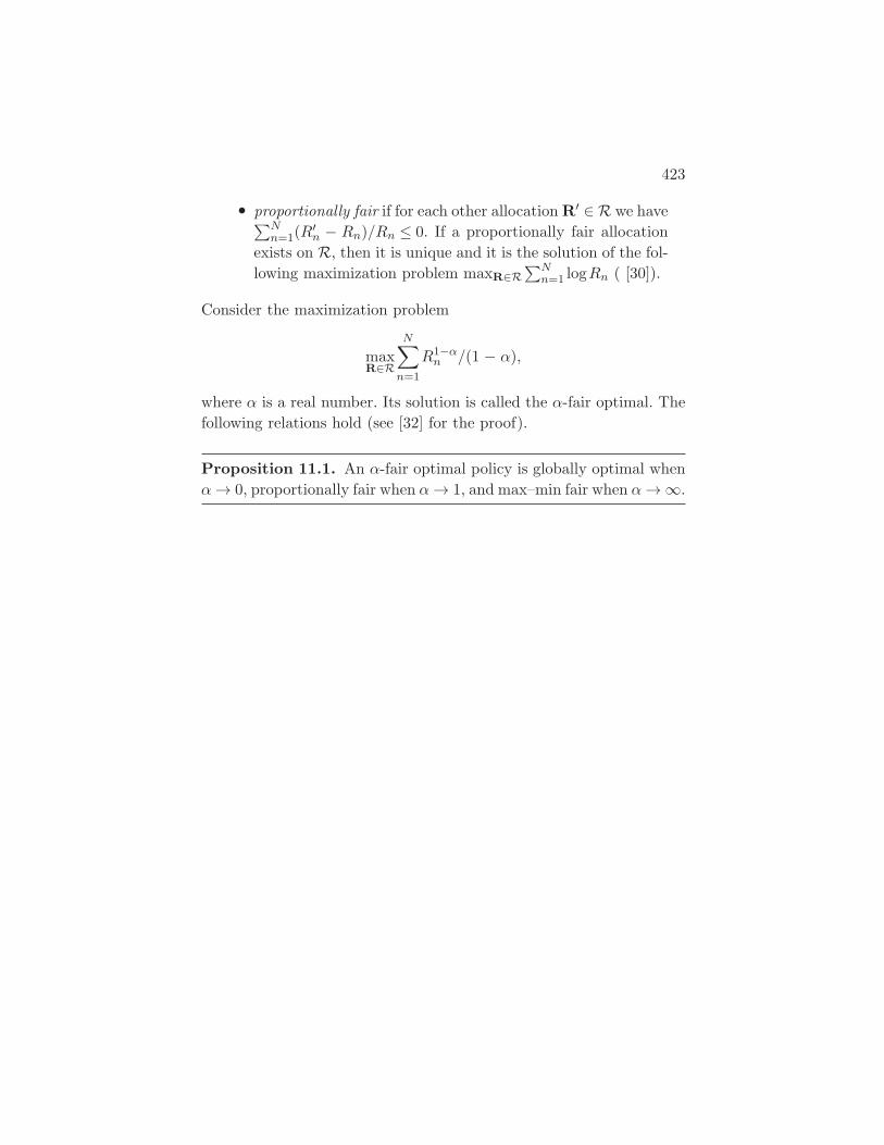
423
• proportionally fair if for each other allocation R′ ∈ R we have∑Nn=1(R
′n − Rn)/Rn ≤ 0. If a proportionally fair allocation
exists on R, then it is unique and it is the solution of the fol-lowing maximization problem maxR∈R
∑Nn=1 logRn ( [30]).
Consider the maximization problem
maxR∈R
N∑n=1
R1−αn /(1 − α),
where α is a real number. Its solution is called the α-fair optimal. Thefollowing relations hold (see [32] for the proof).
Proposition 11.1. An α-fair optimal policy is globally optimal whenα → 0, proportionally fair when α → 1, and max–min fair when α → ∞.

12Lemmas on Fourier Transforms
12.1 Fourier Transforms
For all functions f from R to R we will denote by
f(s) =∫
R
e−2iπtsf(t)dt
its Fourier transform at s ∈ R when it exists.Below, we will make use of the fact that the Fourier transform is
an isometry on the space of square integrable functions (Plancherel–Parseval Theorem; [7]). Namely, for all square integrable functions f
and g, ∫R
f(t)g(t)dt =∫
R
f(s)g(s)ds, (12.1)
where g(s) denotes the complex conjugate of g(s).
12.2 Lemmas
The following lemma and its corollaries establish representations of themass that a (square integrable) density puts on an interval (possibly arandom interval) in terms of the Fourier transform of this density.
424

12.2 Lemmas 425
Lemma 12.1. Let f be a square integrable function. Then for all realnumbers a < b, ∫ b
af(t)dt =
∫R
f(s)e2iπbs − e2iπas
2iπsds. (12.2)
Proof. This immediately follows from the isometry property and fromthe fact that the Fourier transform of the square integrable functiong(t) = (a ≤ t ≤ b) is
g(s) =e−2iπbs − e−2iπas
−2iπs.
Note that if f is a bounded probability density, then it is squareintegrable.
Corollary 12.2. Let X be a non-negative real valued random variablewith a square integrable density f ; let Y be a non-negative and inte-grable real-valued random variable with a square integrable density g.Assume that X and Y are independent. Then
P(X ≤ Y ) =∫
R
f(s)g(s) − 1
2iπsds. (12.3)
Proof. We deduce from (12.2) that the L.H.S. of (12.3) is equal to∫ ∞
0g(y)
∫R
f(s)e2iπys − 1
2iπsdsdy.
Equation (12.3) follows provided one can swap the two integrals. Thisis licit provided the function
(s,y) → g(y)f(s)e2iπys − 1
2iπs
is absolutely integrable. For large |s| this function is integrable as acorollary of the Cauchy–Schwarz inequality and the integrability off2(·), which in view of (12.1) is equivalent to the integrability of |f(s)|2(see also [14, p. 510]). For small |s| the modulus of this function isbounded from above by the function g(y)
∣∣∣f(s)∣∣∣yK for some constant
K so that absolute integrability holds when g has a first moment.

426 Lemmas on Fourier Transforms
For instance, if both X and Y are exponential with parameters λ
and µ, resp., then we can use the Cauchy residue theorem to check that
P(X < Y ) =∫
R
λ
(λ + 2iπs)(µ − 2iπs)ds =
λ
λ + µ
as expected.The next lemma extends the previous representations to the Laplace
transform of the positive part of a real valued random variable.
Lemma 12.3. Let X be a real valued random variable with a squareintegrable density f . Let X+ = max(X,0). Then, for all u > 0,
E(e−uX+) = P(X < 0) +
∫R
f(s)u − 2iπs
ds. (12.4)
Proof. The integral to be evaluated for obtaining the second term is
I(u) =∫ ∞
−∞f(t) (t > 0)e−stdt.
Since the Fourier transform g(s) of the function t → (t > 0)e−ut is1/(u + 2iπs), it follows from the isometry property that
I(u) =∫
R
f(s)u − 2iπs
ds.
A naive use of (12.4) would lead to the result that
P(X > 0) = limu→0
I(u) = −∫
R
f(s)2iπs
ds.
As we shall see below, this is wrong.A first question anyway is the sense to give to the last singular
integral (it is called singular because of the singularity at s = 0).Let φ(.) be some complex valued function which satisfies the follow-
ing assumptions (referred to as A below):
• it is differentiable, with finite derivatives;• it is such that |φ(s)| ≤ 1/|s|µ, when |s| tends to ∞, for some
µ > 0.
12.2 Lemmas 427
One can then give a sense to the singular integral
J =∫
R
φ(s)s
ds, (12.5)
(note that thanks to our assumption on the tail behavior of φ, the onlysingularity that matters here is that at s = 0) as the principal valueform which is defined as
J = limε→0
∫R/[−ε,ε]
φ(s)s
ds. (12.6)
For more on the evaluation of singular integrals and their principalvalue, see [18].
Corollary 12.4. If f is a square integrable probability density with afinite first moment, then for all real numbers a∫ ∞
af(t)dt =
12
− 12iπ
∫R
f(s)e2iπas
sds, (12.7)
where the singular integral is defined as above.
Proof. First, it is enough to prove the formula for a = 0 since the func-tion f(t − a) has for Fourier transform f(s)e2iπas.
The formula for a = 0 is a direct corollary of Lemma 12.3 and of theso-called Sokhotski formula (see [18]) which states that for all functionsφ as above, for all u > 0,
limu→0
∫R
φ(s)s + iu
ds =∫
R
φ(s)s
ds + iπφ(0).
Equation (12.4) and the last relation applied to φ(s) = −(1/2iπ)f(s)immediately give (12.7). Equivalently
limu→0
I(u) =12
−∫
R
f(s)2iπs
ds.
We can use the Sokhotski formula because the Fourier transform of adensity admitting a first moment is differentiable and has finite deriva-tives. In addition the fact that the density is square integrable implies
428 Lemmas on Fourier Transforms
that its Fourier transform is square integrable, so that the tail decayof Assumption A holds.
Here is another proof based on more elementary arguments. Whenletting b go to ∞ in (12.2), the L.H.S. tends to
∫∞0 f(t)dt. We rewrite
the R.H.S. as the sum of three terms
I1 = −∫
R
f(s)2iπs
ds
I2 =∫
R
e2iπbs f(s) − (s ∈ [−ε,+ε])2iπs
ds
I3 =∫
R
e2iπbs − (s ∈ [−ε,+ε])2iπs
ds =12,
where ε is a positive real number.The Riemann–Lebesgue lemma [7] states that for all integrable func-
tions g,
limb→∞
∫R
g(s)e2iπbsds = 0.
So, in order to prove that I2 tends to 0 when b tends to ∞, it is enoughto show that ∫
R
∣∣f(s) − (s ∈ [−ε,+ε])∣∣
2π|s| ds < ∞.
But this follows from the following two bounds:
∫R/[−ε,ε]
∣∣∣f(s)∣∣∣
|s| ds ≤(∫
R/[−ε,ε]
1s2 ds
∫R
∣∣∣f(s)∣∣∣2 ds
) 12
< ∞,
where we used the Cauchy–Shwarz inequality and the fact that f(s) issquare integrable because f(s) is∫
[−ε,ε]
∣∣f(s) − 1∣∣
|s| ds ≤ ε2|f ′(0)|,
where we used that fact that if X has a finite first moment then itsFourier transform is differentiable and has a finite derivative.

13Graph Theoretic Notions
Let (Φ,E) be a connected undirected graph with the set of vertices Φand edges E . The neighbors of vertex (node) x ∈ Φ are defined as theset of nodes y ∈ Φ such that the edge (x,y) ∈ E .
Let w be a collection of non-negative weights associated with theedges of the graph (i.e., a non-negative function described on E). Definethe weight of a subgraph of (Φ,E) as the sum of the weights of its edges.
13.1 Minimum Spanning Tree
A spanning tree of this graph is a subgraph which is a tree and whichconnects all the vertices of this graph. A Minimum Weight SpanningTree (or Minimum Spanning Tree (MST) for short) is a spanning treewith weight no larger than that of all other spanning trees.
Given a connected weighed graph (Φ,E ,w), an MST can be con-structed using Prim’s algorithm:
• Initialize Ψ = x, where x is any node and F = ∅;• Repeat until Ψ = Φ:
429

430 Graph Theoretic Notions
– Choose an edge (u,v) from E with u∈Ψ and v /∈Ψ andwith minimum weight (if there are multiple solutions,pick one arbitrarily);
– Add v to Ψ and (u,v) to F .
The proof of the fact that the output (Ψ = Φ,F) of this algorithm isan MST of (Φ,E ,w) is classical.
Assume the MST is unique. Here are two useful properties.
Lemma 13.1. Assume that for all x, there is a unique neighbor x∗
of x such that w(x,x∗) < w(x,y), for all other neighbors y of x. Then(x,x∗) ∈ F ; i.e., this is an edge of the MST.
Proof. When initializing Prim’s algorithm with x, we see that (x,x∗)is an edge of the MST. Uniqueness concludes the proof.
Lemma 13.2. (Cycle property) For all x and y neighbors, if theedge (x,y) belongs to the MST, there is no sequence of verticesz0,z1, . . . ,zn,zn+1 in Φ, with n ≥ 1, x = z0, y = zn+1, (zk,zk+1) ∈ E forall k = 0, . . . ,n, and for which w(zk+1,zk) < w(x,y), for all k = 0, . . . ,n.
Proof. The above sequence defines a cycle of the graph. Assume (x,y) isin the MST and w(zk+1,zk) < w(x,y), for all k = 0, . . . ,n. If we deleteedge (x,y) in the MST, this breaks it into two subtrees Tx and Ty
with x ∈ Tx and y ∈ Ty. Since each node of Φ is either in Tx or in Ty,there is an integer 0 ≤ k ≤ n such that the nodes z0, . . . ,zk all belongto Tx and the nodes zk+1, . . . ,zn all belong to Ty. Consider now thetree obtained by adding the edge (zk,zk+1) to Tx ∪ Ty. Then this treehas a weight strictly smaller than that of the initial MST, which is acontradiction.
13.1.1 Nearest Neighbor Graph
For any vertex x ∈ Φ call any x∗ ∈ Φ satisfying w(x,x∗) ≤miny∈Φ w(x,y) a w-nearest neighbor of x. We call the nearest neighbor

13.1 Minimum Spanning Tree 431
graph (NNG) of Φ the graph on the set of vertexes Φ for which edgesare drawn between any x and any of its nearest neighbors.
The following statements are simple consequences of the definitionof the NNG and of Lemma 13.1.
Corollary 13.3. Suppose each node x ∈ Φ has a unique nearest neigh-bor. Then the NNG has at most card(Φ) edges. Moreover, NNG is asubgraph of the MST.
13.1.2 Euclidean MST of the Poisson Point Process
Let Φ be a realization of a homogeneous Poisson p.p. on Rd with inten-
sity λ. Consider Φ as the set of vertices of the complete graph (i.e.,for any x,y ∈ Φ, (x,y) ∈ E). Let w(x,y) = |x − y| be the Euclideandistance.
Let K be a compact subset of Rd. Consider the MST (ΦK ,FK)
of (ΦK ,EK ,w), where ΦK = Φ ∩ K and EK = (x,y):x,y ∈ ΦK; it isunique with probability 1. Denote by M = MK(λ) = max(x,y)∈FK
|x −y| the longest edge in the MST of Φ ∩ K.
The following result was proved in [35] for the BM in R2 (and for
the BM in higher dimension on the torus):
Proposition 13.4. Given a unit square K = [−12 , 1
2 ]2 ⊂ R2 and a
homogeneous Poisson p.p. Φ with intensity λ on the plane R2. Denote
by M = M(λ) the longest edge of the MST of Φ ∩ K. Then
limλ→∞
PλπM2 − logλ ≤ u = exp[−e−u] u ∈ R . (13.1)
Proof. We will only give a sketch of the reasoning presented in [35]:Denote by M = M(λ) the longest edges of the NNG of Φ ∩ K. Becausethe NNG is a subgraph of the MST, M ≤ M . Conversely, one getsthat all edges (x,y) of the MST of Φ ∩ K which satisfy the conditionλπ|x − y|2 − logλ > u (we call them u-long) belong to the NNG of
432 Graph Theoretic Notions
Φ ∩ K with a probability converging to 1 when λ → ∞. Consequently
PλπM2 − logλ ≤ u ≤ PλπM2 − logλ ≤ u≤ PλπM2 − logλ ≤ u
+P∃ edge u-long in MST
that is not in NNGand for all u,
limλ→∞
PλπM2 − logλ ≤ u = limλ→∞
PλπM2 − logλ ≤ u .
Now, let us study the following surrogate model of the longest edge inthe NNG. Consider λ (assumed to be an integer) i.i.d. random variablesS1, . . . ,Sλ, with a generic S having for distribution P(S ≥ u) = e−πλu2
,and define M = M(λ) = max(S1 . . . ,Sλ). Note that the distribution ofS corresponds to the distribution of the length of the distance form atypical point of the homogeneous Poisson p.p. with intensity λ to itsnearest neighbor; so the surrogate model ignores the boundary-effectsof the “true” NNG. Moreover, in the true NNG, the number of pointsin K (|K| = 1) is Poisson with mean λ rather than deterministic andequal to λ, and their nearest neighbor distances are not independent.Despite this, it is shown in [35] using the Chen–Stein method that
limλ→∞
PλπM2 − logλ ≤ u = limλ→∞
PλπM2 − logλ ≤ u .
Thanks to independence, it is easy to show that the latter limit of thesurrogate model is equal to
limλ→∞
PλπM2 − logλ ≤ u = limλ→∞
(1 − e−u
λ
)λ= exp[−e−u].
14Discrete Percolation
14.1 Bond Percolation on Zd.
Consider the integer lattice Zd in d dimensions. In what follows, we will
consider d ≥ 2. Denote by L the set of edges joining any two adjacentpoints of Z
d (which are at distance 1 from each other). Consider a familyof random variables X(e)e∈L which are identically distributed withPX(e) = 1 = 1 − PX(e) = 0 = p for some p ∈ [0,1]. We assumethat this family is ergodic with respect to the natural shift on Z
d,however, we do not assume X(e) to be mutually independent. We willsay that the edge e ∈ L is open if X(e) = 1 and closed otherwise. Thismodel is known as bond percolation on L; see Figure 14.1.
Definition 14.1. We say that the bond percolation model percolatesif the set of open edges contains an infinite connected subset.
Denote by C the maximal connected component in the set of openedges containing the origin (as the endpoint of one of the edges). Defineθ(p) = P#C = ∞, where #C denotes the number of edges in theset C.
433
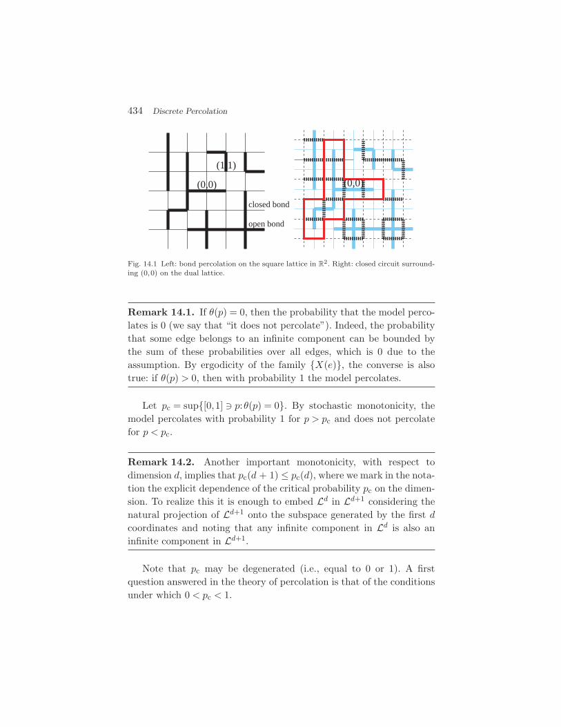
434 Discrete Percolation
(0,0)
(1,1)
closed bond
open bond
(0,0)
Fig. 14.1 Left: bond percolation on the square lattice in R2. Right: closed circuit surround-
ing (0,0) on the dual lattice.
Remark 14.1. If θ(p) = 0, then the probability that the model perco-lates is 0 (we say that “it does not percolate”). Indeed, the probabilitythat some edge belongs to an infinite component can be bounded bythe sum of these probabilities over all edges, which is 0 due to theassumption. By ergodicity of the family X(e), the converse is alsotrue: if θ(p) > 0, then with probability 1 the model percolates.
Let pc = sup[0,1] p:θ(p) = 0. By stochastic monotonicity, themodel percolates with probability 1 for p > pc and does not percolatefor p < pc.
Remark 14.2. Another important monotonicity, with respect todimension d, implies that pc(d + 1) ≤ pc(d), where we mark in the nota-tion the explicit dependence of the critical probability pc on the dimen-sion. To realize this it is enough to embed Ld in Ld+1 considering thenatural projection of Ld+1 onto the subspace generated by the first d
coordinates and noting that any infinite component in Ld is also aninfinite component in Ld+1.
Note that pc may be degenerated (i.e., equal to 0 or 1). A firstquestion answered in the theory of percolation is that of the conditionsunder which 0 < pc < 1.
14.1 Bond Percolation on Zd. 435
14.1.1 Upper Bound for the Critical Probability
We will give now some sufficient condition for pc < 1. We will state andprove the result for d = 2. By Remark 14.2 this will be also a sufficientcondition in all higher dimensions.
Assume thus d = 2. Denote by L′ the shift of the square lattice L bythe half of its side-length horizontally and vertically. The lattice L′ iscalled the dual to L. Note that for each edge e ∈ L there exists a uniqueedge e′ ∈ L′, intersecting e at its center. Thus, one can define uniquelya dual field X ′(e′)e′∈L′ by putting X ′(e′) = X(e); see Figure 14.1.Denote by ρ(n) the number of self-avoiding circuits (closed paths) oflength n in the dual lattice L′ surrounding the origin. The proof of thefollowing results is often referred to as Peierls’s argument (see e.g. [21,pp.16–19]).
Proposition 14.1. Consider the bond percolation model X(e):e ∈ L on the square lattice Z
2. Suppose that for some q (0 ≤ q < 1)
PX(e1) = 0, . . . ,X(en) = 0 ≤ qn (14.1)
for any set of n different edges e1, . . . ,en. If
∞∑n=1
ρ(n)qn < 1 , (14.2)
then the bond percolation model percolates.
Proof. The origin belongs to an infinite connected component iff itis not surrounded by any closed circuit of the dual bond percolationdefined on L′. We will show that this last probability is positive byproving that its complement is strictly less than 1. For this, note that,the probability that there exists a closed circuit surrounding the originis bounded by the expected number of such circuits, which in turn isbounded by
∑∞n=1 ρ(n)qn < 1.
Remark. For the square lattice L on the plane, we have the follow-ing bound: ρ(n) = 0 for n = 1,2,3 and ρ(n) ≤ 4n3n−2 for n ≥ 4. Thus
436 Discrete Percolation
condition (14.1) reads
4/9∞∑4
n(3q)n =4(3q)4(4 − 9q)
9(3q − 1)2 < 1 ,
which is true for q < 0.2075 . . ..
Example 14.2 (Independent bond percolation). In the case ofindependent bond percolation on Z
2, i.e. when X(e):e ∈ L are inde-pendent, condition (14.1) is obviously satisfied by q = 1 − p. Thus con-dition (14.2) is satisfied for p > 1 − 0.2075 · · · = 0.7924 · · · or, in otherwords, pc(2) ≤ 0.7924 · · · . However, in this case some refinement of theproof of Proposition 14.1 can be used to show that percolation holdsprovided the series in (14.2) is only convergent. Indeed, in this case,some number N can be found such that
∑∞n=N ρ(n)qn < 1. Thus, with
positive probability there is no closed circuit surrounding the origin oflength larger than N . Moreover, for any rectangle containing the origin,the configuration of bonds outside the rectangle is independent of theconfiguration of bonds inside the rectangle, and with positive proba-bility all the bonds inside it are open. This shows that the probabilitythat the origin belongs to an infinite open connected component ispositive. This new condition implies that the independent bond perco-lation model percolates for p > 2/3 or, in other words, that pc(2) ≤ 2/3.In fact, in this case, using some more fine arguments concerning thesymmetry of the model one can prove that pc(2) = 1/2 (see e.g. [21,Chapter 9]).
14.1.2 Lower Bound for the Critical Probability;Independent Percolation Case
In the case of independent bond percolation, it is also relatively easyto show that pc(d) > 0 for any d.
Denote by σ(n) = σ(n,d) the number of self-avoiding paths of lengthn on Z
d starting at the origin and let λ(d) = limn→∞(σ(n,d))1/n.
Proposition 14.3. For independent bond percolation on Zd we have
pc(d) ≥ 1/λ(d).
14.2 Independent Site Percolation 437
Proof. Denote by N(n) the number of open paths starting at the originand of length at least n. If the origin belongs to an infinite open paththen obviously for all n, we have N(n) ≥ 1. Thus
θ(p) ≤ PN(n) ≥ 1 ≤ E[N(n)] ≤ pnσ(n)
for all n. If θ(p) > 0 then limn p(σ(n))1/n = pλ(d) ≥ 1, i.e.; p > 1/λ(d),which completes the proof.
The exact value of λ(d) is not known, however, a simple observationgives σ(n,d) ≤ 2d(2d − 1)n−1 and thus λ(d) ≤ 2d − 1.
Concluding what was said about the independent bond percolationwe have proved the following result.
Theorem 14.4. For independent bond percolation on Zd with d ≥ 2
we have 0 < λc < 1.
14.2 Independent Site Percolation
In site percolation, one opens or closes the vertexes of a given graphrather than its edges. Consider again Z
d as the set of vertexes (calledhere “sites”) and edges L defined exactly as in Section 14.1.
Let Y (v)v∈Zd be a family of i.i.d. random variables withPY (v) = 1 = 1 − PY (v) = 0 = p. We will say that the site v ∈ Z
d
is open if Y (v) = 1 and closed otherwise. This model is known as sitepercolation on Z
d; cf. Figure 14.2 Two sites are said adjacent if theyare connected by some edge (bond). A subset of sites is said connectedif the corresponding sub-graph is connected.
Definition 14.2. We say that the site percolation model percolates ifit contains an infinite connected sub-graph with open vertexes.
Denote by Csite the maximal connected sub-graph with open ver-texes containing the origin. Define θsite(p) = P#Csite = ∞, where#Csite denotes the number of vertexes in the set Csite and psite
c =sup[0,1] p : θsite(p) = 0. By stochastic monotonicity, the model per-colates with probability 1 for p > psite
c and does not percolate forp < psite
c .

438 Discrete Percolation
(0,0)
(1,1)
closed site
open site
(0,0)
Fig. 14.2 Left: site percolation on the square lattice in R2. Right: dual bond percolation.
Proposition 14.5. For all d we have psitec < 1; i.e. the site percolation
model percolates for sufficiently large p < 1.
Proof. We will prove this result considering the following dual one-dependent bond percolation. For any edge e ∈ L with end-points in v andw, define X(e) = Y (v)Y (w); i.e., the edge is open iff its end-points areboth open as sites. Obviously, if the dual bond model percolates thenthe original site model percolates as well. By Remark 14.2 it is enoughto prove that the bond model percolates in dimension d = 2. For this wewill use Proposition 14.1. Note that the independence of Y (v) impliesthe following one-dependence of X(e): variables X(e1), . . . ,X(en) aremutually independent if no two edges in e1, . . . ,en have a common ver-tex. Any vertex in any edge in L (in dimension 2) has six edges sharingsome vertex with it. This implies that condition (14.1) is satisfied forq = (1 − p2)n/7 and, by the Remark after Proposition 14.1, condition(14.1) reads
4/9∞∑
n=4
n(3(1 − p2)1/7)n < 1 ,
which is satisfied for sufficiently large p < 1.

References
[1] F. Baccelli and B. Blaszczyszyn, “On a coverage process ranging from theBoolean model to the Poisson Voronoi tessellation, with applications to wirelesscommunications,” Advances in Applied Probability, vol. 33, pp. 293–323, 2001.
[2] F. Baccelli, B. Blaszczyszyn, and F. Tournois, “Downlink capacity andadmission/congestion control in CDMA networks,” in Proceedings of IEEEINFOCOM, San Francisco, 2003.
[3] F. Baccelli, M. Klein, M. Lebourges, and S. Zuyev, “Stochastic geometry andarchitecture of communication networks,” Journal of Telecommunication Sys-tems, vol. 7, pp. 209–227, 1997.
[4] B. Blaszczyszyn, E. Merzbach, and V. Schmidt, “A note on expansion forfunctionals of spatial marked point processes,” Statistics and ProbabilityLetters, vol. 36, pp. 299–306, 1997.
[5] B. Blaszczyszyn and D. Yogeshwaran, “Directionally convex ordering of ran-dom measures, shot-noise fields and some applications to wireless networks,”Advances in Applied Probability, 111, in press.
[6] H. Blichfeldt, “The minimum value of quadratic forms and the closest packingof spheres,” Math. Ann., vol. 101, pp. 605–608, 1929.
[7] P. Bremaud, Mathematical Principles of Signal Processing. New York: Springer,2002.
[8] J. H. Conway and N. J. A. Sloane, Sphere Packings, Lattices and Groups.New York: Springer-Verlag, 1998.
[9] D. J. Daley and D. Vere-Jones, An Introduction to the Theory of PointProcesses. New York: Springer, 1988.
439

440 References
[10] D. J. Daley and D. Vere-Jones, An Introduction to the Theory of PointProcesses. Probability and its Applications, New York: Springer. Volume I:Elementary Theory and Methods, 3, 2005.
[11] D. J. Daley and D. Vere-Jones, An Introduction to the Theory of PointProcesses. Probability and its Applications, New York: Springer. Volume II:General Theory and Structure, 3, 2008.
[12] O. Dousse, F. Baccelli, and P. Thiran, “Impact of interferences on connec-tivity in ad-hoc networks,” IEEE/ACM Transactions on Networking, vol. 13,pp. 425–543, 2005.
[13] O. Dousse, M. Franceschetti, N. Macris, R. Meester, and P. Thiran, “Percola-tion in the signal to interference ratio graph,” Journal of Applied Probability,vol. 43, no. 2, pp. 552–562, 2006.
[14] W. Feller, An Introduction to Probability Theory and its Applications, vol. II.Wiley, 35, 60, 1971.
[15] M. Franceschetti and R. Meester, Random Networks For Communication. 2008.[16] R. Ganti and M. Haenggi, “Interference and outage in clustered wireless ad hoc
networks,” arXiv:0706.2434v1, 111, 2008a.[17] R. K. Ganti and M. Haenggi, “Interference in ad hoc networks with gen-
eral motion-invariant node distributions,” in Proceedings IEEE InternationalSymposium on Information Theory (ISIT’08), Toronto, Canada, July 2008b.
[18] F. Ghakov, Boundary Value Problems. Oxford: Pergamon Press, 1966.[19] E. N. Gilbert, “Random plane networks,” SIAM Journal, vol. 9, pp. 533–543,
iv, 1961.[20] E. N. Gilbert, “Random subdivisions of space into crystals,” The Annals of
Mathematical Statistics, vol. 33, no. 3, pp. 958–972, 1962.[21] G. R. Grimmett, Percolation. New York: Springer-Verlag, 1989.[22] M. Haenggi, J. Andrews, F. Baccelli, O. Dousse, and M. Franceschetti, eds.,
Stochastic Geometry and Random Graphs for Wireless Networks. Special Issueof IEEE JSAC, vol. 67, 2009.
[23] P. Hall, Introduction to the Theory of Coverage Processes. New York: Wiley &Sons, 1988.
[24] J. Illian, A. Penttinen, H. Stoyan, and D. Stoyan, Statistical Analysis andModelling of Spatial Point Patterns. Wiley, 67, 2008.
[25] S. Janson, “Random coverings in several dimensions,” Acta Mathematica,vol. 156, pp. 83–118, 1986.
[26] G. A. Kabatiansky and V. I. Levenshtein, “Bounds for packings on a sphere andin space,” Problemy Peredachi Informatsii, vol. 14, no. 1, pp. 3–25, in Russian,28, 1978.
[27] O. Kallenberg, Random Measures. Berlin: Akademie-Verlag, 6, 8, 1983.[28] L. Kleinrock, Queueing Systems. John Wiley & Sons. iv, 1975.[29] G. Matheron, Random Sets and Integral Geometry. London: John Wiley &
Sons, pp. 43, 45, 1975.[30] A. Maulloo, F. P. Kelly, and D. Tan, “Rate control in communication networks:
Shadow prices, proportional fairness and stability,” Journal of the OperationalResearch Society, vol. 49, pp. 237–252, 1998.

References 441
[31] R. Meester and R. Roy, Continuum Percolation. Cambridge University Press,pp. 39, 54, 108, 1996.
[32] J. Mo and J. Walrand, “Fair end-to-end window-based congestion control,”IEEE/ACM Transactions on Networking, vol. 9, no. 5, pp. 556–567, 123, 2000.
[33] J. Møller, Lectures on Random Voronoi Tessellations. vol. 87 of Lecture Notesin Statistics, New York: Springer-Verlag, pp. 60, 67, 1994.
[34] A. Okabe, B. Boots, K. Sugihara, and S. N. Chiu, Spatial Tessellations —Concepts and Applications of Voronoi Diagrams. (second ed.), Wiley, p. 67,2000.
[35] M. Penrose, “The longest edge of the random minimal spanning tree,” TheAnnals of Applied Probability, vol. 7, no. 2, pp. 340–361, 132, 133, 1997.
[36] M. D. Penrose and J. E. Yukich, “Limit theory for random sequential packingand deposition,” The Annals of Applied Probablity, vol. 12, no. 1, pp. 272–301,29, 2002.
[37] C. Pugh and M. Shub, “Ergodic elements of ergodic actions,” Compositio Math-ematica, vol. 23, no. 1, pp. 115–122, 1971.
[38] B. Radunovic and J.-Y. Le Boudec, “A unified framework for max–min andmin–max fairness with applications,” in 40th Annual Allerton Conference onCommunication, Control, and Computing, p. 123, 2002.
[39] Y. Rozanov, Markov Random Fields. New York: Springer, p. 17, 1982.[40] R. Senoussi, J. Chadoeuf, and D. Allard, “Weak homogenization of point pro-
cesses by space deformations,” Advances in Applied Probability, vol. 32, pp. 948–959, 12, 2000.
[41] R. Serfozo, Introduction to Stochastic Networks. New York: Springer, p. 4, 1999.[42] D. Stoyan, W. Kendall, and J. Mecke, Stochastic Geometry and its Applications.
Chichester: Wiley, pp. 67, 77, 87, 96, 1995.[43] D. Stoyan and M. Schlather, “Random sequential adsorption: Relationship to
dead leaves and characterization of variability,” Journal of Statistical Physics,vol. 100, pp. 969–979, 29, 2000.
[44] S. Torquato, O. U. Uche, and F. H. Stillinger, “Random sequential additionof hard spheres in high euclidean dimensions,” Physical Review E, vol. 74,no. 061308, p. 29, 2006.
[45] S. Weber, X. Yang, J. G. Andrews, and G. de Veciana, “Transmission capacityof wireless ad hoc networks with outage constraints,” IEEE Transactions onInformation Theory, vol. 51, no. 12, pp. 4091–4102, 111, 2005.
[46] S. Zuyev, Strong Markov Property of Poisson Processes and Slivnyak Formula,vol. 185 of Lecture Notes in Statistics. Springer, pp. 77–84, 67, 2006.
[47] S. Zuyev, Stochastic Geometry and Telecommunications Networks. OxfordUniversity Press, New Perspectives in Stochastic Geometry, p. 67, 2009.
Table of Mathematical Notation andAbbreviations
|X| Euclidean norm of vector X.|B| Lebesgue measure of set B ∈ B.\ set difference.〈X,Y 〉 scalar product of vectors X and Y .A parameter of the OPL attenuation models.a.s. almost surely.A(X) (resp. An(X)) radial point map at X (resp. time–space
point map at X and at time n).Ad(X) (resp. Ad,n(X)) d-directional point map at X (resp.
time–space point map at X and at time n).B the Borel σ-algebra of the Euclidean space.BX(r) ball of center X and radius r.β attenuation exponent of the OPL
attenuation models.CX(Φ) Voronoi cell of point X w.r.t. the p.p. Φ.C(X,M)(Φ) SINR cell of point X w.r.t. the marks
(fading, threshold, power, etc.) M and thep.p. Φ.
D the destination node (in routing context;Part V in Volume II).
442
References 443
e (resp. e(n)) indicator of MAC channel access (resp. attime n).
E expectation.E0 expectation w.r.t. the Palm probability.εx Dirac measure at x.F (resp. F (n)) fading variable (resp. at time n).GSINR the SINR graph.GSINR the time–space SINR graph.GI General fading.
GIW+GI/GI Kendall-like notation for a wireless cell or
network.iff if and only if.i.i.d. independently and identically distributed.IΦ shot noise field associated with the point
process Φ.K(β) constant associated with Rayleigh fading SN.
See (2.26 in Volume I) and (16.9 inVolume II)
L(X) length to the next hop from point X in arouting algorithm.
L(X) local delay at node X.l(.) attenuation function of the OPL models.LΦ Laplace functional of the p.p. Φ.LV Laplace transform of the random variable V .λ the intensity parameter of a homogeneous
Poisson p.p.Λ(.) the intensity measure of a Poisson p.p.L.H.S. left hand side.M exponential random variable (or Rayleigh
fading).M space of point measures.µ the mean fading is µ−1.N the non-negative integers.N (µ,σ2) the Gaussian law of mean µ and variance σ2
on R.

444 References
N C(0,σ2) the complex vauled Gaussian law.O the origin of the Euclidean plane (in routing
context; Part V in Volume II).p medium access probability in Aloha.P (X) progress from point X towards destination
in a routing algorithm.P probability.P0 Palm probability.pc probability of coverage.Φ point process.R
d Euclidean space of dimension d.S the source node (in routing context; Part V
in Volume II).R.H.S. right hand side.T threshold for SINR.Var Variance.V (X) (resp. V (X,n)) set of neighbors of X in GSINR (resp. of
(X,n) in GSINR).W (resp. W (n)) thermal noise (resp. at time n).Z the relative integers.

Index
3G, see third generation cellularnetwork 296
access point, 296, 347ad hoc network, 263, 271, 336, 345adaptive coding, 22, 26, 50, 68, 102admission control, 127, 138, 151Aloha, 123, 205, 206, 271, 287
opportunistic, 44, 206spatial, 17
antennaazimuth beam-width, 258
antipodal signaling, 277atom, 264attenuation
omni-directional, 257, 306azimuth, 257, 260, 310
ball property, 215, 236base station, 126, 147, 296baseband signal, 267, 273beam-width of antenna, 258bipolar model, 18, 122
blockingprobability, 148, 149rate, 152
BM, 163, see Boolean model 319percolation, 163
bond percolation, 433Boolean model (BM), 319
clump, 333connectivity
in a finite window, 329homogeneous, 322percolation, 332time–space, 111
bounded set, 261broadcast, 61BS, see base station 126
Campbellformula, 31, 277, 278, 388
higher order, 395, 415reduced, 277, 280
measure, 276higher order, 414reduced, 276, 414
445

446 INDEX
Campbell–Little–Mecke formula, seeCampbell formula 277
Campbell–Matthesformula, 285, 340, 419, 420measure, 285, 295, 418
capacity functional, see RAC ... 321capture, 21CDF, see contact distribution
function 325spherical, 325
CDMA, 126, see code divisionmultiple access 288, 378
admission control, 138power control, 129rate control, 138virtual load, 134
cell rejection probability, 142chip, 280clump, see BM ... 333cluster head, 201, 295coherence
bandwidth, 275distance, 261, 308, 313time, 263, 275
collision, 286complete independence, 265concentrator, 296connectivity
of a BM in a finite window, seeBM ... 329
contact distribution function, 325contention domain, 286continuum percolation, 329counting measure, 261covariance function, see RAC ... 324coverage probability
CSMA, 122of a RAC, 326
CPR, see cell rejection probability142
CSMA, 112, see carrier sensemultiple access 288, 299
back-off, 113, 288busy medium, 112contention domain, 112, 288
detection threshold, 112, 114,123
idle medium, 112
data rate, 279dead end, 219dead end problem, 183Delaunay
graph, 162, 181, 291triangulation, 345
delay, 167end-to-end, 214, 221, 242, 248local, 82, 211, 214
delay rate, 213, 223delay spread, 261density
of progress, 71of successful transmissions, 15,
123of throughput, 15
digital communication model, 11, 26,167
Dijkstra’s algorithm, 168, 238, 292Dirac measure, 261direct-sequence spread-spectrum, 280directed spanning forest, 187directional
progress, 70distribution
circular-symmetric, 272complex-valued Gaussian, 273Gaussian, 269, 277isotropic, 272multinomial, 263phase type, 359
diversity, 99DL, see downlink 127Doppler
shift, 262spread, 263, 275
downlink, 129, 296, 307DSF, see directed spanning forest
187, see directed spanning forest196
dynamic programming, 168, 292

INDEX 447
ergodicity, 189, 287, 288, 420Erlang loss formula, 148error probability, 278ESN, see extremal shot-noise 316Euclidean distance approximation,
177, 200exchange formula, 343, 348exclusion zone, 287
fading, 313fast, 12, 83, 208, 220, 242flat, 275, 276, 278, 280heavy tailed, 99lognormal, 99Nakagami, 157, 270Rayleigh, 34, 48, 49, 220, 254,
270Rician, 34, 49, 254, 270slow, 12, 83, 208, 242Weibull, 99
far-field, 28, 257, 264forest, 201Fourier transform, 424
Gaussian vector, 272goodput, 284graph
Boolean connectivity, 329Delaunay, 162, 171, 174, 175,
177, 181, 200, 291nearest neighbor, 431random geometric, 162, 178,
181, 238, 329SINR, 156, 163, 178, 401
connectivity, 63, 156, 401time–space, 209, 235
strip, 188, 219transmission range, 162, 291
graph distance, 167
hard core p.p., 296, 300Hex, see honeycomb model 137honeycomb model, 136, 137, 149,
307, 343
i.m.p.p., 114, see independentlymarked p.p. 292
independent nearest receiver, 56independent receiver model, 54infinite connected component, 163,
178, 332, 334, 335, 337, 401,402, 404
infinite server queue, 148INR, see independent nearest
receiver 56intensity
critical, 333, 404measure, 262, 278of a stationary p.p., 285, 418
interference, 21cancellation factor, 128, 284,
404field, 306
isotropy, 418
Johnson–Mehl cell, 363, 375, 399jump vector, 161
Kendall-like notation, 23for SINR cell, 356, 380for SINR cell with fading, 361for SINR coverage, 384for SN, 307, 314
Kingman’s theorem, 170, 222, 223
Lambert function, 76local delay, 82, 211, 215, 219
multicast, 105phase transition, 85, 90Shannon, 102
locally finite measure, 261
m.p.p., see marked point process 291MAC, 165, see medium access
control 286Aloha, 17
MANET, see mobile ad hoc network273, 290, 307
Aloha, 18nearest neighbor, 58nearest receiver, 58Poisson bipolar model, 18, 122
MANET receiver model, 55, 207

448 INDEX
MAP, see medium access probability17, 45
mark of a point process, 190, 417mass transport principle, 63, 68Matern p.p., 296
CSMA, 114hard core, 296, 297
matched filter, 281, 288measure
Campbell m. of a p.p., 276mean m. of a p.p., 276
medium accesscontrol, 286probability, 17
MHC, see Matern hard core 297,418
minimal spanning tree, 179minimum spanning tree, 429MNN, see MANET nearest neighbor
58MNR, see MANET nearest receiver
58mobile ad hoc network, 273, 290mobility, 13, 101, 273
high, 83, 274moment measure
factorial, 413higher order, 395, 413, 416
MST, 179multi-layer coding, 68multicast, 61, 68, 105, 186, 295
one-to-many, 295multipath fading, 261multiple access
carrier sense, 288code division, 288frequency division, 284time division, 287
MWR, see minimal weight routing168, 186
Nakagami fading, 157, 270near-field, 28nearest neighbor
distance to, 280graph, 431in a cone, 98
nearest receiverin a cone, 80
networkcellular, 136, 296, 307, 347
third generation, 296delay tolerant, 13interference limited, 95, 220,
356, 396mobile ad hoc, 290noise limited, 93, 220, 356, 396sensor, 181, 201, 295with periodic infrastructure,
100, 207NNG, see nearest neighbor graph
431non-outage, 21NR, see routing; nearest receiver
routing 56number of hops, 161, 211, 248
omni-directional path-loss, 257, 306OPL, 20, see omni-directional path
loss 306opportunism, 44, 165opportunistic
Aloha, 44, 206choice of receiver, 70routing, 206, 235
orthogonal signature sequence, 283,378
p.p., see point process 261packet, 18, 287
capture, 11, 205velocity, 215, 224
packet model, 11, 82, 205Painleve–Kuratowski convergence,
363, 365, 372, 397, 399Palm
distribution, 189, 278higher order, 415of marks, 295, 418reduced, 277, 415
version of a p.p.reduced, 280
Palm–Matthes distribution, 285,289, 340, 343, 419, 420

INDEX 449
paradoxFeller’s, 164, 342routing, 164, 251
passband signal, 267path-gain
distance and angle dependent,257
level-set, 260path-loss
exponent, 258, 307omni-directional, 257, 306
Peierls’ argument, 407, 435percolation
Boolean, 183, 329first passage, 213, 222of a BM, 332, see BM 404of bonds, 174, 405, 406, 407,
433of sites, 171, 435, 437SINR, 156, 179, 402
phase transitionwireless contention, 85, 90, 95
point average, 289point map, 161, 180, 183, 216, 236
directional, 186, 187, 195, 215,245
radial, 186, 214, 236time–space, 165, 213, 216, 236,
245point measure, 261, 417point process, 261
n-th factorial power, 395, 412n-th power, 412ergodic, 23, 63, 287, 288isotropic, 418Laplace functional, 266marked, 291, 417
independently, 292stationary, 294
point transformation, 272Poisson, 262
homogeneous, 262simple, 264stationary, 284, 417superposition, 269thinning, 270
Poisson p.p., 262homogeneous, 262Palm distribution
k fold, 118Poisson-Voronoi model, 136pole capacity, 65, 380power control, 15, 126, 288
cellular network, 128feasibility, 129, 148feasibility probability, 142, 148
price of anarchy, 164, 200Prim’s algorithm, 429principal value, 357, 427processing gain, 280progress, 18, 30, 58, 161, 165, 188,
214directional, 70, 199, 245modified, 74radial, 191
pseudo-noise signature sequence, 280PV, see Poisson-Voronoi model 136
QAM, see quadrature amplitudemodulation 267
quadrature amplitude modulation,267
RAC, see random closed set 318radial spanning tree, 181radiation pattern, 258, 310random
closed ball, 319closed set (RAC), 318
capacity functional, 321,357
contact distributionfunction, 325
covariance function, 324,360
coverage probability, 326translation invariant, 323volume fraction, 323
compact set, 282cross-fading model, 21, 70, 135,
315sequential addition, 300walk, 273waypoint, 273

450 INDEX
rate control, 127, 138, 145Rayleigh fading, 34, 48, 49, 254, 270,
276, 278, 280, 308response function, 300, 353, 364Restart algorithm, 91, 98, 102retention function, 270, 332Rician fading, 34, 49, 254, 270rotation operator, 418route average, 163, 166, 198, 219,
224, 248, 289time–space, 206, 215
routing, 161best hop, 54, 181, 186, 235cross-layer, 53, 69, 206, 235directional, 195, 245, 246, 247geographic, 180, 185, 251, 294greedy, 165, 180, 235largest bottleneck, 178layer-aware, 205, 216minimal delay, 176minimal weight, 168, 291multicast, 54, 193, 295multihop, 161, 290, 336nearest receiver, 55, 56, 58next-in-strip, 183, 188, 219opportunistic, 54, 69, 165, 206,
235point-to-point, 181, 291, 295radial, 190, 295shortest path, 165, 168, 291smallest hop, 53, 58, 80, 182,
186, 187, 192, 248time–space, 165, 205, 215time-space, 402
routing paradox, 164, 199, 251routing table, 180, 294RP, see radiation pattern 258RST, see radial spanning tree 181,
186, 192, 197internal, 201local, 201
S–D, see source–destination pair 291saturated hard balls, 299SBD, see spatial birth and death
process 149scale invariance, 177, 190
scaling lawGupta–Kumar, 29, 246
scaling laws, 29, 67, 69scatterer, 261self-avoidance, 222, 229shadowing, 84Shannon
capacity, 11, 26, 40, 50, 158multicast, 68
shift operator, 420shot-noise, 21, 84, 209, 300
extremal, 75, 116, 119, 316field, 301, 353, 405time–space, 315
signal to interference and noise ratio,353
signal to noise ratio, 362signature, 280, 281, 283singular integral, 357, 427SINR, 282, see signal to interference
and noise ratio 353cell, 353, 377, 401connectivity graph, 63coverage, 21coverage process, 383graph, 156, 163, 178, 401modified, 128, 134neighbor, 62, 209, 216, 229target, 128
site percolation, 437Slivnyak’s theorem, 278, 293, 386
higher order, 416Slivnyak-Mecke theorem, see
Slivnyak’s theorem 278slow fading, 208small scale fading, 263SN, see shot noise 21, see shot-noise
300SNR, 278, see signal to noise ratio
362SNR cell, 364source–destination pair, 291spanning tree, 429spatial
average, 63, 86, 102, 117, 164,197, 199, 206, 287

INDEX 451
birth and death process, 149Erlang loss formula, 148, 152reuse, 18, 287
spatial reusefactor, 42
spectral radius, 130, 289sphere packing, 298, 300standard stochastic scenario
for SINR cell, 355for SN, 167, 307
stopping set, 173, 282strip graph, 188, 219strong Markov property, 60, 232, 282subadditive process, 170, 222, 223successful reception, 21
TDMA, see Time Division multipleaccess 287
tessellation, 338theorem
Kingman’s, 170, 222, 223Slivnyak’s, 190, 278, 280, 281,
293, 332, 386higher order, 416
thermal noise, 20, 80, 129, 353space independent, 356, 384time independent, 356
thinning, 36, 114, 270, 297independent, 20
throughput, 158, 178, 247tilt, 257time average, 102time constant, 213time slot, 12time–space
graph, 229loss, 147path, 210
routing, 165, 215shot-noise, 82, 315SINR graph, 209
time-spacerouting, 402
trafficconstant bit rate, 26elastic, 138
translation operator, 417transmission range, 163, 178, 238,
291transport, 30, 58tree
spanning, 295radial, 181
typical node, 22
UL, see uplink 127universal marks, 419uplink, 132, 296
virtual power, 20, 62, 122, 308, 313volume fraction, 298, 323, 395Voronoi
cell, 136, 201, 339fundamental region, 347
flower, 184, 347neighbor, 162, 186, 291, 345,
346tessellation, 155, 184, 338
VT, see Voronoi tessellation 338
WiFi, 122, 125, 290mesh, 181, 295