stochastic dominance relationships between stock and index … annual meetings... · 2016-11-07 ·...

Stochastic Dominance Relationships between Stock and Index Futures:

International Evidences

Zhuo Qiao*

Faculty of Business Administration, University of Macau Title: Assistant Professor. Email: [email protected]

Wing-Keung Wong

Department of Economics, Hong Kong Baptist University

Title: Professor. Email: [email protected]

Joseph K W, Fung

Department of Finance & Decision Sciences, Hong Kong Baptist University

Title: Professor. Email: [email protected]

Abstract Adopting a stochastic dominance (SD) approach, this paper examines the dominance relationships between stock indices and their corresponding index futures in the 10 countries, including 6 developed countries and 4 developing countries. Our findings show that there is no SD relationship between spot and futures markets in the developed countries, indicating the nonexistence of cross-market arbitrage profit or possible gains in expected utilities for investors. By contrast, our findings show that in the developing countries, spot dominates futures for risk averters while futures dominate spot for risk seekers in the sense of the second and third order SD, indicating the existence of gains in expected utilities for risk averters (seekers) when switching from investing futures (spot) to spot (futures). Our results provide insight to understand the investor’s behaviour in these markets and are useful to help investors to make decisions.

Keywords stochastic dominance, risk averter, risk seeker, stock, index futures

EFM Classification: 380, 720, 420

∗ Corresponding author and paper presenter. Address: Department of Finance and Business Economics, Faculty of Business Administration, University of Macau, Avenida Padre Tomás Pereira, Taipa, Macau, China, ZIP, 999078. Tel: +853 8397 4166; fax: +853 2883 8320; e-mail: [email protected]. Research field based on EFM code: 380 and 720.

1

1. Introduction

The relationship between the stock index and its underlying stock index futures is a very

important topic which has been the subject of numerous empirical studies. One of the major lines

of enquiry in the literature on index futures is about their roles in improving market efficiency.

Researchers such as Black and Scholes (1972), Roll (1977), and Biais and Hillion (1994) argue

that the introduction of such financial derivatives could help to improve information transmission

among investors and make the financial market complete and more efficient. Under perfectly

efficient markets, new information is impounded simultaneously into stock and index futures

markets. Thus, two markets will adjust fully and instantaneously to reflect all available relevant

information.

But in real markets, factors such as liquidity, various transaction costs, information asymmetry

and other market restrictions may produce market frictions. Futures markets could reflect new

information more quickly than do spot markets given their inherent leverage, low transaction

costs, and lack of short-sale restrictions (Tse, 1999). As a result, there exist the possible

opportunities for cross-market index arbitrage.1 One way to examine the possible existence of

arbitrage opportunity is to analyze whether there is any lead-lag relationship between the two

markets. If one market leads the other, arbitrage opportunity would exist (Fleming et al., 1996).

Many studies have investigated this by applying various econometrics models, see, for example,

Kawaller et al. (1987), Stoll and Whaley (1990), Chan (1992), Abhyankar (1995), Fleming et al.

(1996), Tse (1999), and Zhong et al. (2004) and many others. However, their analyses are

usually conducted under certain assumptions about market return distributions, such as normal

distribution, which is well-known to be violated in reality.

To circumvent the potential limitations of previous lead-lag perspective in examine cross-market 1 From the traditional theoretical point of view, the existence of an arbitrage strategy violates assumptions of the efficiency of the market.

2

arbitrage opportunity, this paper adopts a non-parametric stochastic dominance (SD) approach to

investigate the stochastic dominance relationship between stock and index futures in the 10

developed and developing financial markets. The SD approach provides a new way to examine

the existence of arbitrage opportunity across index futures market and its underling stock market.

Furthermore, this approach also enables us to investigate the preference of investors (both risk

averters and seekers) from the perspective of utility maximization, which is interesting to both

academics and practitioners. In addition, the SD approach could also enable investors to examine

market efficiency and market rationality in the futures and spot markets.

Compared with other methods, the key attraction of the SD approach is its nonparametric

orientation on the entire distributions comparison. Specifically, SD criteria do not require any

assumption on returns distribution. For example, returns can display time series dependence and

conform to any distribution. The advantage of SD analysis over parametric tests becomes

apparent when the assets return distributions are non-normal because the SD approach does not

require any assumption about the nature of the distribution and therefore it can be used for any

type of distribution. Further more, SD endorses the minimum restrictions on investors’ utility

functions. The underlying utility functions can be any standard linear utility function satisfying

von-Neumann-Morgenstern axioms and a variety of nonlinear utility functions based on

substantially weaker axioms (Fishburn, 1989). Machina (1982), Starmer (2002), and Wong and

Ma (2008) show that stochastic dominance criteria are also meaningful for a range of non-

expected utility theories of choice under uncertainty.2 The SD approach has been regarded as one

of the most useful tools to rank investment prospects (see, for example, Levy 1992) as the 2 Most of the existing literature has employed the conventional parametric tests such as mean-variance (MV) criterion and the CAPM statistics. These approaches are derived assuming the von Neumann-Morgenstern (1944) quadratic utility function and that returns are normally distributed (Feldstein, 1969; Hanoch and Levy, 1969). Thus, the reliability of performance comparisons using the MV criterion and CAPM analysis depends on the degree of non-normality of the returns data and the nature of the (non-quadratic) utility functions (Beedles, 1979; Schwert, 1990; Fung and Hsieh, 1999). SD incorporates information on the entire return distribution, rather than the first two moments as used by employing the MV and CAPM.

3

ranking of the assets has been proven to be equivalent to utility maximization for the preferences

of risk averters and risk seekers (Tesfatsion, 1976; Stoyan, 1983; Li and Wong, 1999).

Our empirical results show that the dominance relationships between these two assets in the

developed countries differ from those in the developing countries. In the developed countries,

there is no SD relationship between spot and futures markets for the first three orders. This

indicates the nonexistence of cross-market arbitrage profit or possible gains in expected utilities

for both risk averters and risk seekers. By contrast, we find that in the developing countries spot

dominates futures for risk averters while futures dominate spot for risk seekers in the sense of the

second and third order stochastic dominance, inferring that risk averters will enhance their

expected utilities by switching from investing futures to spot while risk seekers will achieve this

by switching from investing spot to futures. Our results provide insight to understand the

investor’s behaviour in these markets and are useful to help investors to make decisions.

The rest of this paper is organized as follows. We will briefly discuss the theory of SD for risk

averters and risk seekers in Section 2. Section 3 introduces the Davidson and Duclos test (here

below DD test, 2000) for stochastic dominance, and discusses test implementation issues.

Section 4 describes the dataset and presents descriptive statistics. The SD empirical results are

presented and analyzed in Section 5. The final section contains some concluding remarks.

2. Stochastic Dominance Theory

SD theory initially developed by Hadar and Russell (1969), Hanoch and Levy (1969), and

Rothschild and Stiglitz (1970) is one of the most useful tools in investment decision-making

under uncertainty to rank investment prospects. Let F and G be the cumulative distribution

functions (CDFs), and f and g be the corresponding probability density functions (PDFs) of

two investments, X and Y , respectively, with common support [ , ]a b where a < b. Define

4

0 0A DH H h= = , ( ) ( )1

xA Aj ja

H x H t dt−= ∫ and ( ) ( )1

bD Dj jx

H x H t dt−= ∫ (1)

for ,h f g= ; ,H F G= ; and 1,2,3j = . We call the integral AjH the thj order ascending

cumulative distribution function (ACDF) and the integral DjH the thj order descending

cumulative distribution function (DCDF) for H F= and G .and for j = 1, 2 and 3.

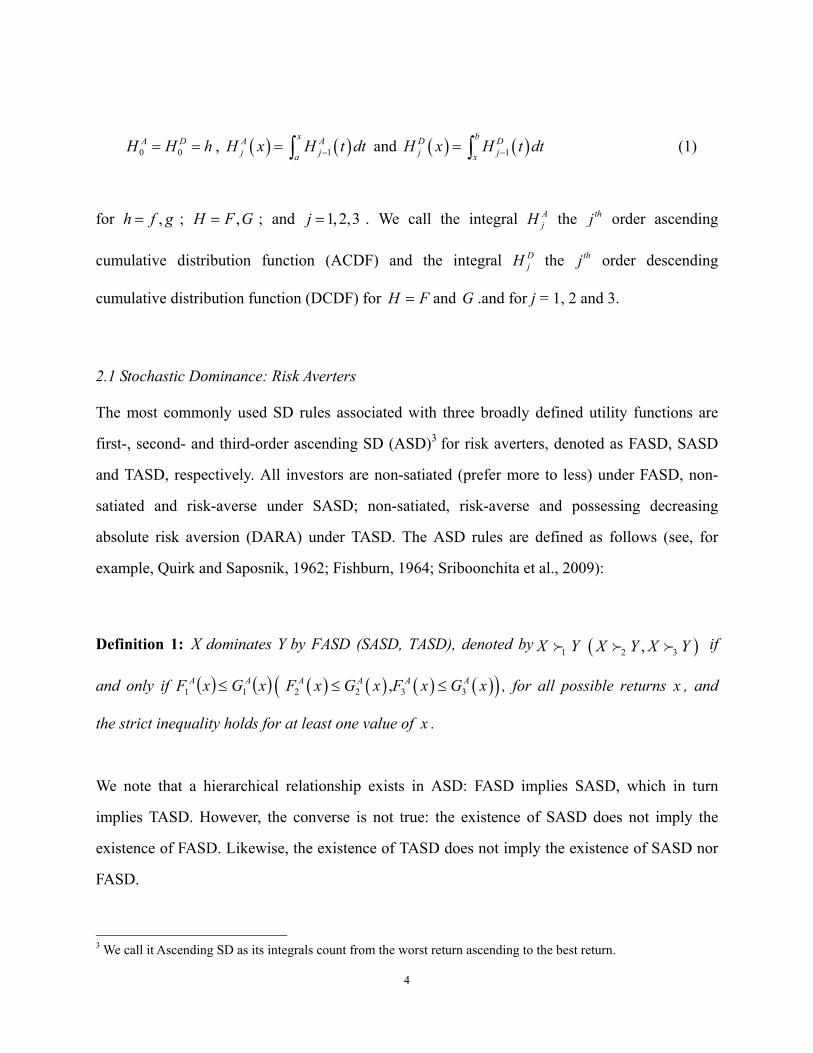
2.1 Stochastic Dominance: Risk Averters

The most commonly used SD rules associated with three broadly defined utility functions are

first-, second- and third-order ascending SD (ASD)3 for risk averters, denoted as FASD, SASD

and TASD, respectively. All investors are non-satiated (prefer more to less) under FASD, non-

satiated and risk-averse under SASD; non-satiated, risk-averse and possessing decreasing

absolute risk aversion (DARA) under TASD. The ASD rules are defined as follows (see, for

example, Quirk and Saposnik, 1962; Fishburn, 1964; Sriboonchita et al., 2009):

Definition 1: X dominates Y by FASD (SASD, TASD), denoted by1X Y ( )2 3,X Y X Y if

and only if ( ) ( )xGxF AA11 ≤ ( ) ( ) ( ) ( )( )2 2 3 3 ,A A A AF x G x F x G x≤ ≤ , for all possible returns x , and

the strict inequality holds for at least one value of x .

We note that a hierarchical relationship exists in ASD: FASD implies SASD, which in turn

implies TASD. However, the converse is not true: the existence of SASD does not imply the

existence of FASD. Likewise, the existence of TASD does not imply the existence of SASD nor

FASD.

3 We call it Ascending SD as its integrals count from the worst return ascending to the best return.

5

2.2 Stochastic Dominance: Risk Seekers

Wong and Li (1999) and others show that stochastic dominance rules apply to risk seekers, with

the preferences reversed to those of risk averters under certain conditions. Whereas SD for risk

averters works with the ACDF which count from the worst return to the best return, SD for risk

seekers works with the DCDF which counts from the best return descending to the worst return

(Stoyan, 1983; Wong and Li, 1999; Post and Levy 2005). Hence, SD for risk seekers could be

called descending SD (DSD). We have the following definition for DSD (see, for example,

Meyer, 1977; Li and Wong, 1999; Anderson, 2004).

Definition 2: X dominates Y by FDSD (SDSD, TDSD)) denoted by 1X Y ( )2 3,X Y X Y if

and only if ( ) ( )xGxF DD11

≥ ( ) ( ) ( ) ( )( )2 2 3 3 , D D D DF x G x F x G x≥ ≥ , for all possible returns x , the

strict inequality holds for at least one value of x ; where FDSD (SDSD, TDSD) stands for first-

order (second-order, third-order) descending SD.

All investors are non-satiated under FDSD; non-satiated and risk-seeking under SDSD; non-

satiated, risk-seeking and possessing increasing absolute risk seeking under TDSD. Similarly, the

theory of DSD is related to the utility maximization for risk seekers (Stoyan 1983, Li and Wong

1999, Wong 2007) and the hierarchical relationship for ASD also exists in DSD.

To make a choice between two assets X and Y, risk averters will compare their corresponding jth

order ASD integrals and choose X if AjF is smaller for j = 1,2,3. On the other hand, risk seekers

will compare their corresponding jth order DSD integrals and choose X if DjF is bigger (Wong

and Chan, 2008; Sriboonchita, et al., 2009).

SD analysis is important because investigating the SD relationship across different financial assts

is equivalent to examining the choice of assets by utility maximization under SD theory. The

6

existence of SD implies that the investor’s expected utility is always higher when the investor

holds the dominant asset than when s/he holds the dominated asset, and consequently, the

dominated asset would not be chosen. For instance, the dominance of X over Y by FASD (SASD,

TASD) indicated in Definition 1 is equivalent to the preference of X over Y by the first- (second-,

third-) order risk-averters (Quirk and Saposnik 1962), whereas the dominance of X over Y by

FDSD (SDSD, TDSD) indicated in Definition 2 is equivalent to the preference of X over Y by the

first- (second-, third-) order risk-seekers (Li and Wong 1999, Anderson 2004, Wong 2007).

Finally, we note that investment X stochastically dominates investment Y by FASD (FDSD), if

and only if there is an arbitrage opportunity between X and Y , such that risk averters (seekers)

will increase their expected wealth as well as their expected utilities if their investments are

shifted from Y to X . They could make huge profits by setting up zero dollar portfolios to

exploit this opportunity. On the other hand, if investment X stochastically dominates investment

Y by SASD or TASD (SDSD or TDSD), risk averters (seekers) will increase their expected

utilities but not their expected wealth if their investments are shifted from Y to X (Bawa, 1978;

Jarrow, 1986; Falk and Levy, 1989).

3. Davidson and Duclos (DD) Test

The early work of Beach and Davidson (1983) examines dominance at the first order. More

recently, several methods have been proposed for testing for stochastic dominance of other

orders (Anderson (1996), Davidson and Duclos (DD, 2000) Barrett and Donald ( 2003) and

Linton et al. ( 2005)). Some literatures like Wei and Zhang (2003), Tse and Zhang (2004), and

Lean et al. (2008) show that the DD test is powerful and parsimonious. It is also easy to compute.

Hence, we adopt DD statistics the DD test for the empirical work in this paper.4

4 As the SD test developed by Linton et al. (LMW 2005) has been shown to be one of the best, in this paper we also conduct the LMW test to analyse the data. As the results from LMW test draw the same conclusion as those from the

7

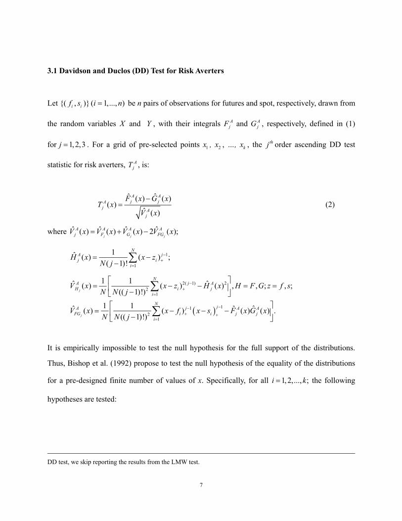
3.1 Davidson and Duclos (DD) Test for Risk Averters

Let {( if , is )} ( 1,..., )i n= be n pairs of observations for futures and spot, respectively, drawn from

the random variables X and Y , with their integrals AjF and A

jG , respectively, defined in (1)

for 1,2,3j = . For a grid of pre-selected points 1x , 2x , …, kx , the thj order ascending DD test

statistic for risk averters, AjT , is:

ˆˆ ( ) ( )

( )ˆ ( )

A Aj jA

j Aj

F x G xT x

V x

−= (2)

where ˆ ˆ ˆ ˆ( ) ( ) ( ) 2 ( );j j j

A A A Aj F G FGV x V x V x V x= + −

1

1

1ˆ ( ) ( ) ;( 1)!

NA jj i

iH x x z

N j−

+=

= −− ∑

( )

2( 1) 22

1

112

1

1 1ˆ ˆ( ) ( ) ( ) , , ; , ;(( 1)!)

1 1 ˆˆ ˆ( ) ( ) ( ) ( ) .(( 1)!)

j

j

NA j AH i j

i

NjA j A A

FG i i j ji

V x x z H x H F G z f sN N j

V x x f x s F x G xN N j

−+

=

−−+ +

=

= − − = = −

= − − − −

∑

∑

It is empirically impossible to test the null hypothesis for the full support of the distributions.

Thus, Bishop et al. (1992) propose to test the null hypothesis of the equality of the distributions

for a pre-designed finite number of values of x. Specifically, for all 1, 2,..., ;i k= the following

hypotheses are tested:

DD test, we skip reporting the results from the LMW test.

8

( ) ( ) ( ) ( )( ) ( ) ( ) ( )

0

1

2

: ( ) ( ) , for all ;

: ( ) ( ) for some ;

: for all , for some ;

: for all , for some .

A Aj i j i i

A AA j i j i i

A A A AA j i j i i j i j i i

A A A AA j i j i i j i j i i

H F x G x x

H F x G x x

H F x G x x F x G x x


=

≠

≤ <

≥ >

(3)

Accepting either 0H or AH implies non-existence of any SD relationship between X and Y, non-

existence of any arbitrage opportunity between these two markets, neither of these markets is

preferred to the other. If 1AH ( 2AH ) of order one is accepted, X (Y) stochastically dominates Y (X)

at first-order. In this situation and under certain regularity conditions5, an arbitrage opportunity

exists and any non-satiated investor will be better off if he/she switches from the dominated asset

to the dominant one. On the other hand, if 1AH ( 2AH ) is accepted for order two (three), a

particular market stochastically dominates the other at second- (third-) order. In this situation,

arbitrage opportunity does not exist, and switching from one asset to another could only increase

the risk averters’ expected utilities, but not their expected wealth (Jarrow, 1986; Falk and Levy,

1989; Wong et al. 2008).

3.2 Davidson and Duclos Test for Risk Seekers

To test SD for risk seekers, we modify the DD statistic for risk averters to be the descending DD

test statistic, DjT , such that:

ˆˆ ( ) ( )

( )ˆ ( )

D Dj jD

j Dj

F x G xT x

V x

−= (4)

5 Refer to Jarrow (1986) for the conditions.

9

where ˆ ˆ ˆ ˆ( ) ( ) ( ) 2 ( );j j j

D D D Dj F G FGV x V x V x V x= + −

1

1

1ˆ ( ) ( ) ;( 1)!

ND jj i

iH x z x

N j−

+=

= −− ∑

( )

2( 1) 22

1

112

1

1 1ˆ ˆ( ) ( ) ( ) , , ; , ;(( 1)!)

1 1 ˆˆ ˆ( ) ( ) ( ) ( ) ;(( 1)!)

j

j

ND j DH i j

i

NjD j D D

FG i i j ji

V x z x H x H F G z f sN N j

V x f x s x F x G xN N j

−+

=

−−+ +

=

= − − = = −

= − − − −

∑

∑

in which the integrals DjF and D

jG are defined in (1) for 1,2,3j = . For 1,2,..., ,i k= the

following hypotheses are tested for risk seekers:

( ) ( ) ( ) ( )( ) ( ) ( ) ( )

0

1

2

: ( ) ( ) , for all ;

: ( ) ( ) for some ;



D Dj i j i i

D DD j i j i i

D D D DD j i j i i j i j i i

D D D DD j i j i i j i j i i

H F x G x x

H F x G x x



=

≠

≥ >

≤ <

Similar to the case for risk averters, accepting either 0H or DH implies non-existence of any SD

dominance relationship between X and Y, non-existence of any arbitrage opportunity between

these two markets, neither of the asset is preferred to the other. If 1DH ( 2DH ) of order one is

accepted, asset X (Y) stochastically dominates Y (X) at first-order. In this situation, an arbitrage

opportunity exists and any non-satiated investor will be better off and obtains higher expected

utilities as well as greater expected wealth if he/she switches his/her investment from the

dominated asset to the dominant one. On the other hand, if 1DH or 2DH is accepted at order two

(three), a particular asset stochastically dominates the other at second- (third-) order. In this

situation, arbitrage opportunity does not exist, and switching from one asset to another could

only increase the risk seekers’ expected utilities, but not their expected wealth (Sriboonchita et

10

al., 2009).

3.3 Implementation Issues

Both DD tests for risk averters and risk seekers compare distributions at a finite number of grid

points. Various studies examine the choice of grid points. For example, Tse and Zhang (2004)

show an appropriate choice of k for reasonably large samples ranges from 6 to 15. Too few grids

will miss information on the distributions between any two consecutive grids (Barrett and

Donald, 2003), and too many grids will violate the independence assumption required by the

SMM distribution (Richmond, 1982). In order to make the comparisons comprehensive without

violating the independence assumption, we follow Fong et al. (2005, 2008), Gasbarro et al. (2007)

and Wong et al. (2008) to make 10 major partitions with 10 minor partitions within any two

consecutive major partitions in each comparison, and show the statistical inference based on the

SMM distribution for k = 10 and infinite degrees of freedom6. In other words, DD test statistics

are computed over a grid of 100 points on the distributions of the daily spot and futures returns.

This allows the consistency of both the magnitude and sign of the DD statistics between any two

consecutive major partitions to be examined. The percentage of DD statistics which are

significantly negative or positive at the 5% significance level, based on the asymptotic critical

value of 3.254 of the SMM distribution are computed.

4. Data

The dataset consists of 10 major national stock indices and their corresponding index futures in

6 Refer to Lean et al. (2008) for explanation in detail.

11

the global financial market, including the USA (S&P 500 index), Canada (S&P/TSX index), UK

(FTSE 100 index), Germany (DAX index), France (CAC 40 index), Japan (Nikkei 225 index),

Taiwan (TAIEX index), Hong Kong (Hang Seng index), Singapore (Strait Times index), and

Brazil (BOVESPA index). Our sample covers January 3, 2000 through December 31, 2007. For

the purpose of a robustness check, the sample is divided into two sub-samples that have roughly

the same number of observations in each sub-period. The first sub-sample covers the period

January 3, 2000 – December 31, 2003, and the second covers the period January 2, 2004 –

December 31, 2007.7 As most of the countries are basically in bear market in the first sub-period

and in bull run in the second sub-period, our SD implication in the sub-periods could infer the

results for bear market and bull run. Daily log returns Ri,t = ln (Pi,t / Pi,t-1) for both the spot (S)

and futures (F) indices are calculated where Pi,t is the daily index at day t for index i with i = S

(Spot) and F (Futures), respectively.

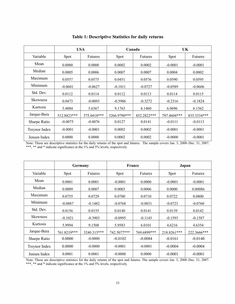
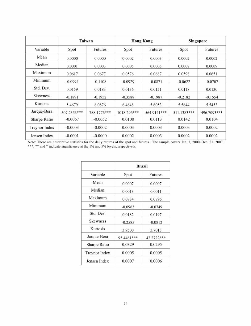
Table 1 contains descriptive statistics for the daily returns of stock and index futures of these

countries. It is shown that, for all countries, the mean and variance of daily returns of stock and

index futures are similar. For the CAPM measures8, since both returns have similar values on

Sharpe ratios, Treynor and Jensen indices, the information drawn from the CAPM statistics

cannot draw any preference between the spot and futures markets. Moreover, returns of both

stock and futures have higher kurtosis than normality. In addition, the highly significant Jarque-

7 For the reason of the availability of the data, the data for Singapore starts from June 29, 2000. 8 Readers may refer to Sharpe (1964), Treynor (1965) and Jensen (1969) for the statistics.

12

Bera (J-B) statistics shown in Table 1 further confirm that both sets of returns are non-normal.

This infers that the results from mean-variance and CAPM statistics may draw misleading

inference (Fung and Hsieh, 1999).9

< Table 1 here >

5. Empirical Results

5.1 SD Analysis for Risk Averters

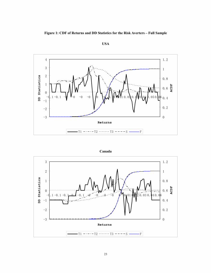
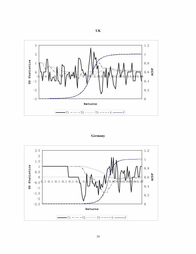
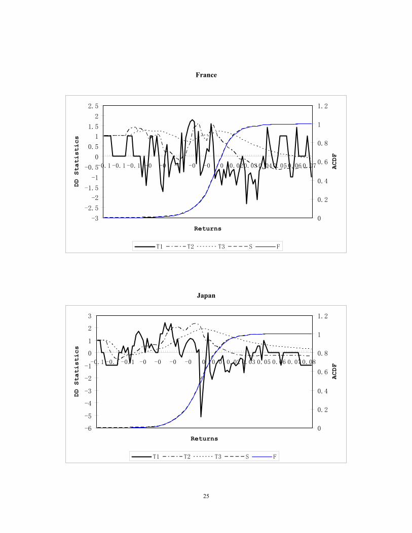
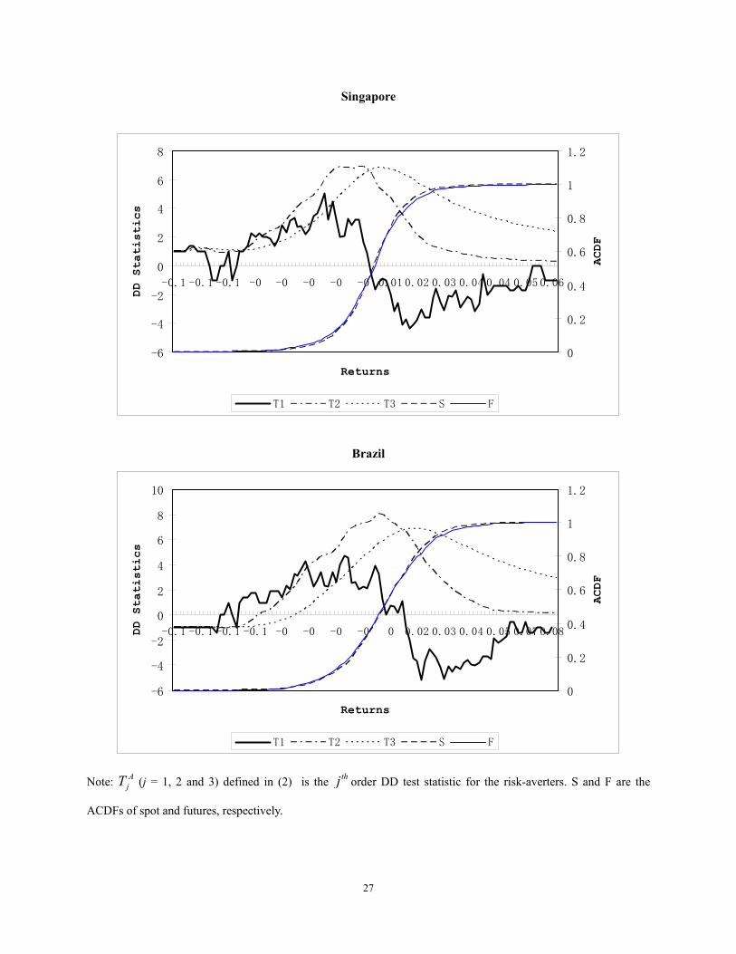
We first depict in Figure 1 the CDFs of the returns for both spot and futures and their

corresponding ascending DD statistics, AjT (j=1, 2, 3), for risk averters for all the 10 countries in

our sample. If futures (spot) dominate spot (futures) in the sense of FASD, then we should

observe the CDF of futures (spot) returns should lie below that of the spot (futures) in Figure 1.

From Figure 1, we find that this does not occur in any of the countries, inferring that there are no

FSD relationship and thus no arbitrage opportunity in any of the developed countries as well as

in any of the developing countries.

Nonetheless, from Figure 1, it is clear that the SD relationships between spot and futures markets

in the six developed countries (i.e. USA, Canada, UK, Germany, France and Japan) are different

from those in the four developing countries (i.e. Taiwan, Hong Kong, Singapore and Brazil). For

the six developed countries, it is shown that CDFs of both spot and futures returns almost

coincide with each other over the entire return distributions and 1AT runs “randomly” in the

positive domain as well as in the negative domain . On the other hand, for the four developing

9 Though it is well-known that if normality does not hold, CAPM statistics may lead to biased results (Hanoch and Levy (1969), Falk and Levy (1989), and Fung and Hsieh (1999)), we still provide CAPM statistics here only for reference. When calculate these statistics, the 3-month U.S. T-bill rate and the Morgan Stanley Capital (MSCI) world index return are used as the proxy for the risk-free return rate and the global market return, respectively.

13

countries in our sample, Figure 1 reveals that CDFs of spot and futures cross with each other and

1AT changes its sign around zero across the negative return domain and the positive return

domain with some significant portions (i.e. the absolute value of 1AT is greater than 3.254) in

both domains, indicates that spot dominates futures on the downside risk whereas futures could

dominate spot on the upside profit range for the developing countries but not for the developed

countries. Furthermore, different from those for the developed countries, both 2AT and 3

AT for the

developing countries are significantly positive for some portions with no significant negative

values, inferring there exist SASD and TASD between spot and futures markets in the

developing countries but not in the developed countries.

< Figure 1 here >

To verify this more formally, we employ the first three orders of the ascending DD statistics, AjT

( 1, 2,3j = ), for the two series, X and Y for futures and spot, respectively, on each country and

display the results in Table 2. From the table, we find that, for all six developed countries, there

is no SD relationship between spot and futures markets for all three orders. This suggests that

there is no cross-market index arbitrage opportunity and switching from one market to the other

could neither increase the risk averters’ expected wealth nor their expected utilities.

In contrast to the finding above for the developed countries, Table 2 provides very different

results for the developing countries. In general, the findings from all four developing countries

are very similar to each other. It is shown that there exist some SD relationships between spot

and futures markets in these countries. Taking the Taiwan as an example, from Table 2, we find

that 16% (17%) of 1AT is significantly positive (negative). Considering this and the evolution

pattern of 1AT depicted in Figure 2, we conclude that, though there is no FASD between spot and

14

futures markets, spot dominates futures significantly in the downside risk, while the futures

dominate significantly spot in the upside profit. The absence of the FASD over the entire return

distribution leads us to focus the analysis on higher orders to compel utility interpretations in

terms of investors’ risk aversion and decreasing absolute risk aversion (DARA), respectively.

Table 2 displays that 40% (64%) of the 2AT ( 3

AT ) is significantly positive and no 2AT ( 3

AT ) DD

statistic is significantly negative at the 5% level. Hence, we conclude that risk averters prefer

spot over futures significantly in the sense of both SASD and TASD, implying that, by switching

from investing futures to spot, risk averters could increase the expected utilities (Jarrow, 1986;

Falk and Levy, 1989; Wong et al. 2008).

< Table 2 here >

5.2 SD Analysis for Risk Seekers

So far, if we apply the existing ASD tests on the issue, we could only draw conclusion on the

preferences for risk averters, but not for risk seekers. Thus, an extension of the SD test for risk

seekers is necessary as discussed in the previous sections. This section provides subsequent

discussions to illustrate the applicability of DSD test to draw preferences for risk seekers. In

order to examine the risk-seekers’ preferences, DSD theory for risk-seeking has been developed

(refer to the Section 2.2). In this paper, we adopt the DD test for risk seekers, namely descending

DD statistics, DjT (j = 1, 2 and 3), for the first three orders of risk seekers (refer to the Section

3.2).

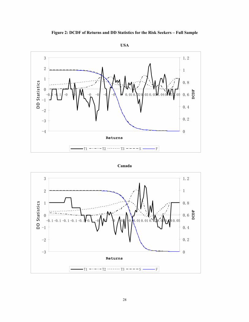
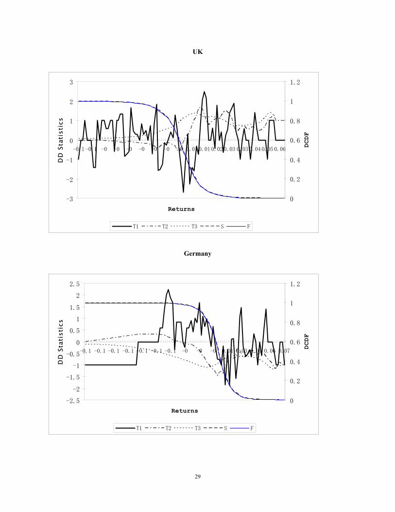
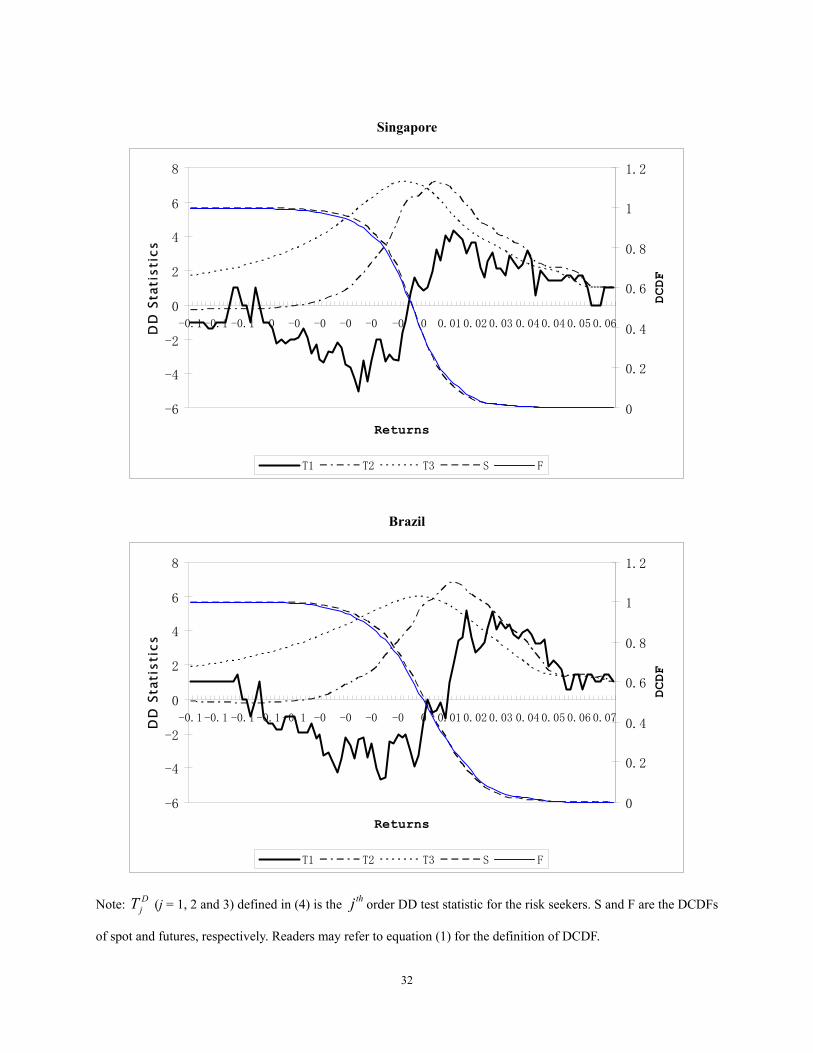
We exhibit in Figure 2 the descending CDFs of the returns for both spot and futures and their

corresponding descending DD statistics, DjT (j=1, 2, 3), for risk seekers of the 10 countries in our

sample. Figure 2 shows that, for the six developed countries, (first order) DCDFs of both spot

15

and futures returns almost coincide with each other. This indicates that there is no FDSD

between the spot and futures markets in these developed countries.

However, for the four developing countries, Figure 2 displays that DCDFs of spot and futures

cross with each other and 1DT changes its sign around zero across the negative return domain and

the positive return domain with some significant portions (i.e. the absolute value for 1DT is

greater than 3.254) in both domains. This suggests that, there is no FDSD relationship between

the two returns and risk seekers may prefer spot to futures in the in the downside risk while

prefer futures in the upside profit. In addition, different from those for the developed countries,

both 2AT and 3

AT for the developing countries are positive and significant (higher than 3.254) for

some reasonably large portions, inferring there exist SDSD and TDSD between spot and futures

markets in these developing countries.

< Figure 2 here >

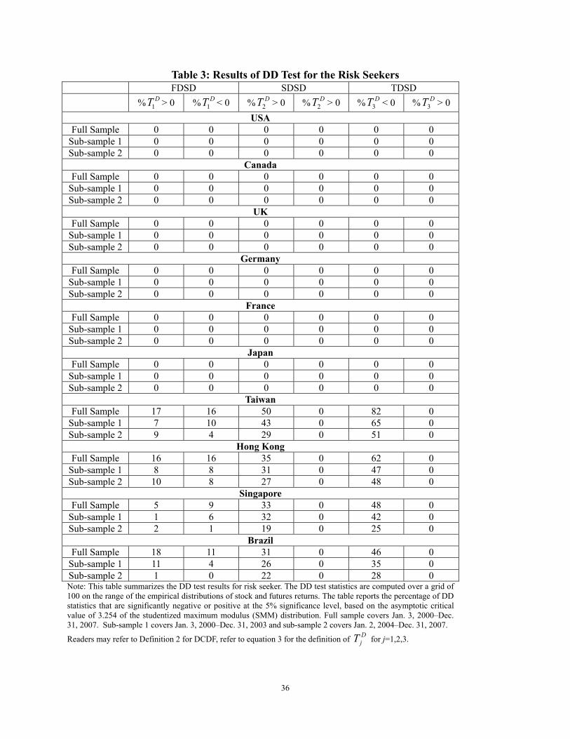
Table 3 provides the result of a formal analysis of DD test for risk seekers. Since the number of

positive significant DjT and negative significant D

jT ( 1, 2,3j = ) are both zero for all six developed

countries, we conclude that there is no SD relationship between spot and futures markets for all

three orders in these markets. This suggests that there does not exist index arbitrage opportunity

between these two markets in these countries and switching from investing one market to

investing another could neither increase the risk seekers’ expected wealth nor their expected

utilities.

However, in a sharp contrast to the developed countries, Table 3 displays that there are SD

relationships between spot and futures markets in the developing countries. Again taking the

16

Taiwan as an example, from Table 3, we find that 17% (16%) of 1DT is significantly positive

(negative). Considering this and the evolution pattern of 1DT depicted in Figure 2, we conclude

that, though there is no FDSD between spot and futures markets, spot dominates futures

significantly in the downside risk, while the futures dominate significantly spot in the upside

profit. As there is no FDSD, we examine DjT for the second and third orders. Table 3 shows that

50% (82%) of 2DT ( 3

DT ) are significantly positive while no 2DT ( 3

DT ) is significantly negative.

This leads us to conclude that the futures dominate the spot significantly in the sense of both

SDSD and TDSD, and consequently, risk seekers could maximize their expected utilities by

switching from investing spot to investing futures (Sriboonchita et al., 2009).10

< Table 3 here >

6. Conclusions

This paper adopts a stochastic dominance approach to examine the dominance relationships

between the stock indices and their corresponding index futures in the 10 countries, including 6

developed countries and 4 developing countries. We find the dominance relationships between

these two assets in the developed countries differ from those in the developing countries. In USA,

Canada, UK, Germany, France and Japan, we do not find any stochastic dominance relationship

between spot and futures markets for the first three orders for both risk averters and risk seekers.

This indicates the nonexistence of cross-market arbitrage profit or possible gains in expected

utilities for both risk averters and risk seekers. By contrast, in the developing countries like

10 Tables 2 and 3 also provide the robustness test results for two sub-samples. As indicated there, the findings are consistent with each other.

17

Taiwan, Hong Kong, Singapore and Brazil, spot dominates futures for risk averters while futures

dominate spot for risk seekers in the sense of the second and third order stochastic dominance,

indicating the existence of gains in expected utilities for risk averters (seekers) when switching

from investing futures (spot) to spot (futures). Our results provide insight to understand the

investor’s behaviour in these markets and are useful to help investors to make decisions.

18

References Abhyankar, A. H., 1995. Return and volatility dynamics in the FTSE 100 stock index and stock index futures markets. Journal of Futures Markets 15, 457-488. Anderson, G.., 1996. Nonparametric tests of stochastic dominance in income distributions. Econometrica 64, 1183 – 1193. Anderson, G.., 2004. Toward an empirical analysis of polarization. Journal of Econometrics 122, 1-26. Barrett, G., Donald, S., 2003. Consistent tests for stochastic dominance. Econometrica 71, 71-104. Bawa, Vijay S., 1978. Safety-first, stochastic dominance, and optimal portfolio choice. Journal of Financial and Quantitative Analysis 13, 255-271. Beedles, W. L. 1979. Return, dispersion and skewness: synthesis and investment strategy. Journal of Financial Research, 71-80. Biais, B., Hillion, P. 1994. Insider and liquidity trading in stock and options markets. Review of Financial Studies 7, 743-780.

Bishop, J.A., Formly, J.P., Thistle, P.D., 1992. Convergence of the South and non-South income distributions. American Economic Review 82, 262-272. Black, F., Scholes, M., 1972. The valuation of option contracts and a test of market efficiency, Journal of Finance 27, 339-417. Chan, K., 1992. A further analysis of the lead-lag relationship between the cash market and stock index futures market. Review of Financial Studies 5, 123-152. Davidson, R., Duclos, J-Y., 2000. Statistical inference for stochastic dominance and for the measurement of poverty and inequality. Econometrica 68, 1435-1464. Falk, H., Levy, H., 1989. Market reaction to quarterly earnings' announcements: A stochastic dominance based test of market efficiency. Management Science 35, 425-446. Feldstein, M.S., 1969. Mean variance analysis in the theory of liquidity preference and portfolio

19

selection, Review of Economics Studies 36, 5-12. Fishburn, P.C., 1964. Decision and Value Theory, New York. Fleming, J., Ostdiek, B., Whaley, R. E., 1996. Trading costs and the relative rate of price discovery in stock, futures and option markets. Journal of Futures Markets 16, 353-387. Fong, W.M., Lean, H.H., Wong, W.K., 2008. Stochastic dominance and behavior towards risk: the market for internet stocks. Journal of Economic Behavior and Organization 68(1), 194-208. Fong, W.M., See, K.H., 2002. A Markov switching model of the conditional volatility of crude oil futures prices. Energy Economics 24, 71-95. Fong, W.M., See, K.H., 2003. Basis variations and regime shifts in the oil futures market. The European Journal of Finance 9, 499–513. Fong, W.M., Wong, W.K., Lean, H.H., 2005. International momentum strategies: A stochastic dominance approach. Journal of Financial Markets 8, 89–109. Fung, W., Hsieh, D.A., 1999. Is mean-variance analysis applicable to hedge funds? Economic

Letters, 62, 53-58. Gasbarro, D., Wong, W.K., Zumwalt, J.K., 2007. Stochastic dominance analysis of iShares. European Journal of Finance 13, 89-101. Gertler, M.L., 1988. Financial Structure and Aggregate Economic Activity: An Overview. Journal of Money, Credit and Banking 20, 559-588. Hadar J., Russell, W.R., 1969. Rules for ordering uncertain prospects. American Economic Review 59, 25-34. Hanoch, G., Levy, H., 1969. The efficiency analysis of choices involving risk. Review of Economic studies 36, 335-346. Hammoudeh, S., Li, H., 2004. The impact of the Asian crisis on the behavior of US and international petroleum prices. Energy Economics 26, 135–160. Jarrow, R., 1986. The relationship between arbitrage and first order stochastic dominance. Journal of Finance 41, 915-921.

20

Jensen, M.C., 1969. Risk, the pricing of capital assets and the evaluation of investment portfolios. Journal of Business 42, 167-247. Kahneman, D., Tversky, A., 1979. Prospect theory of decisions under risk, Econometrica 47, 263-291. Kawaller, I., Koch, P., Koch, T., 1987. The temporal price relationship between S& P 500 futures and S&P 500 index. Journal of Finance 42, 1309-1329. Lean, H.H., Wong, W.K., Zhang, X., 2008. The sizes and powers of some stochastic dominance tests: A Monte Carlo study for correlated and heteroskedastic distributions. Mathematics and Computers in Simulation 79, 30-48. Levy H., 1992. Stochastic dominance and expected utility: Survey and analysis, Management Science 38, 555-593. Levy, H., Levy, M., 2004. Prospect theory and mean-variance analysis. Review of Financial Studies 17, 1015-1041. Li, C. K., Wong, W.K., 1999. Extension of stochastic dominance theory to random variables. RAIRO Recherche Opérationnelle 33(4), 509-524. Linton, O., Maasoumi, E., Whang, Y-J., 2005. Consistent testing for stochastic dominance under general sampling schemes. Review of Economic Studies 72, 735-765. Markowitz, H.M., 1952. Portfolio selection. Journal of Finance 7, 77-91. McFadden, D., 1989. Testing for stochastic dominance. In: T.B. Fomby and T.K. Seo, (Eds.), Studies in the Economics of Uncertainty. Springer Verlag, New York. Meyer, J., 1977. Second degree stochastic dominance with respect to a function. International Economic Review 18, 476-487. Post, T., Levy, H., 2005. Does risk seeking drive asset prices? A stochastic dominance analysis of aggregate investor preferences and beliefs. Review of Financial Studies 18(3), 925-953. Quirk, J.P., Saposnik, R., 1962. Admissibility and measurable utility functions. Review of Economic Studies 29, 140-146. Richmond, J., 1982. A general method for constructing simultaneous confidence intervals. Journal of the American Statistical Association 77, 455-460.

21

Rochschild, M., Stiglitz, J.E., 1970. Increasing risk I. A definition. Journal of Economic Theory 2, 225-243. Roll, R., 1977. An Analytic Valuation Formula for Unprotected American Call Options on Stocks with Known Dividends. Journal of Financial Economics 5, 251-258. Schwert, G., William, 1990. Stock returns and real activity: a century of evidence. Journal of Finance 45(4), 1237-1257. Sharpe, W.F., 1964. Capital asset prices: Theory of market equilibrium under conditions of risk. Journal of Finance 19, 425-442. Sriboonchita, S., Wong, W.K., Dhompongsa, S., Nguyen, H.T., 2009. Stochastic dominance and applications to finance, risk and economics, Chapman and Hall/CRC, Taylor and Francis Group, Boca Raton, Florida, USA. Stoll, H. R., Whaley, R. E., 1990. The dynamics of stock index and stock index futures returns. Journal of Financial and Quantitative Analysis 25, 441-468. Stoyan, D., 1983. Comparison methods for queues and other stochastic models. New York: Wiley. Tesfatsion, L., 1976. Stochastic dominance and maximization of expected utility. Review of Economic Studies 43, 301-315. Treynor, J.L., 1965. How to rate management of investment funds. Harvard Business Review 43, 63-75. Tse, Y. K., 1999. Price discovery and volatility spillovers in the DJIA index and futures markets. Journal of Futures Markets 19, 911–930 Tse, Y.K., Zhang, X., 2004. A Monte Carlo investigation of some tests for stochastic dominance. Journal of Statistical Computation and Simulation 74, 361-378. Tversky, A., Kahneman, D., 1992. Advances in prospect theory: Cumulative representation of uncertainty. Journal of Risk and Uncertainty 5, 297-323. von-Neumann, J., Morgenstern, O., 1944. Theory of games and economic behavior, Princeton

University Press, Princeton N.J.

22

Wilson, B., Aggarwal, R., Inclan, C., 1996. Detecting volatility changes across the oil sector. Journal of Futures Markets 16, 313–320. Wong, W.K. 2006. Stochastic dominance theory for location-scale family, Journal of Applied Mathematics and Decision Sciences, 2006, 1-10. Wong, W.K., 2007, Stochastic dominance and mean-variance measures of profit and loss for

business planning and investment, European Journal of Operational Research 182, 829-843. Wong, W.K., Chan, R.H., 2008. Markowitz and prospect stochastic dominances, Annals of Finance 4(1), 105-129. Wong, W.K., Li, C.K., 1999. A note on convex stochastic dominance theory, Economics Letters, 62, 293-300. Wong, W.K. Ma, C., 2008. Preferences over location-scale family, Economic Theory 37(1), 119-146. Wong, W.K., Phoon, K.F., Lean, H.H., 2008. Stochastic dominance analysis of Asian hedge funds, Pacific-Basin Finance Journal 16(3), 204-223. Zhong, M., Darrat, A., Otero, R., 2004. Price discovery and volatility spillovers in index futures markets: Some evidencefrom Mexico. Journal of Banking & Finance 28, 3037-3054.

23

Figure 1: CDF of Returns and DD Statistics for the Risk Averters – Full Sample

USA

-3

-2

-1

0

1

2

3

4

-0.1 -0.1 -0 -0 -0 -0 -0 -0 0.01 0.01 0.02 0.03 0.04 0.05 0.06

Returns

DD S

tati

stic

s

0

0.2

0.4

0.6

0.8

1

1.2

ACDF

T1 T2 T3 S F

Canada

-3

-2

-1

0

1

2

3

-0.1 -0.1 -0.1 -0.1 -0.1 -0 -0 -0 -0 0 0.01 0.02 0.03 0.04 0.06

Returns

DD S

tati

stic

s

0

0.2

0.4

0.6

0.8

1

1.2

ACDF

T1 T2 T3 S F

24

UK

-3

-2

-1

0

1

2

3

-0.1 -0.1 -0 -0 -0 -0 -0 -0 0.01 0.02 0.02 0.03 0.04 0.05 0.06

Returns

DD S

tati

stic

s

0

0.2

0.4

0.6

0.8

1

1.2

ACDF

T1 T2 T3 S F

Germany

-2.5

-2

-1.5

-1

-0.5

0

0.5

1

1.5

2

2.5

-0.1 -0.1 -0.1 -0.1-0.1 -0.1 -0.1 -0 -0 -0 0.01 0.03 0.04 0.06 0.07

Returns

DD S

tati

stic

s

0

0.2

0.4

0.6

0.8

1

1.2AC

DF

T1 T2 T3 S F

25

France

-3

-2.5

-2

-1.5

-1

-0.5

0

0.5

1

1.5

2

2.5

-0.1 -0.1 -0.1 -0 -0 -0 -0 -0 0 0.020.03 0.04 0.05 0.06 0.07

Returns

DD S

tati

stic

s

0

0.2

0.4

0.6

0.8

1

1.2

ACDF

T1 T2 T3 S F

Japan

-6

-5

-4

-3

-2

-1

0

1

2

3

-0.1 -0.1 -0.1 -0 -0 -0 -0 0 0.01 0.02 0.03 0.05 0.06 0.07 0.08

Returns

DD S

tati

stic

s

0

0.2

0.4

0.6

0.8

1

1.2

ACDF

T1 T2 T3 S F

26

Taiwan

-6

-4

-2

0

2

4

6

8

10

-0.1 -0.1 -0.1 -0.1 -0.1 -0 -0 -0 -0 0 0.02 0.03 0.04 0.05 0.07

Returns

DD S

tati

stic

s

0

0.2

0.4

0.6

0.8

1

1.2

ACDF

T1 T2 T3 S F

Hong Kong

-8

-6

-4

-2

0

2

4

6

8

10

12

-0.1 -0.1 -0.1 -0.1 -0 -0 -0 -0 -0 0.01 0.02 0.03 0.04 0.06 0.07

Returns

DD S

tati

stic

s

0

0.2

0.4

0.6

0.8

1

1.2

ACDF

T1 T2 T3 S F

27

Singapore

-6

-4

-2

0

2

4

6

8

-0.1 -0.1 -0.1 -0 -0 -0 -0 -0 0.01 0.02 0.03 0.04 0.04 0.05 0.06

Returns

DD S

tati

stic

s

0

0.2

0.4

0.6

0.8

1

1.2

ACDF

T1 T2 T3 S F

Brazil

-6

-4

-2

0

2

4

6

8

10

-0.1 -0.1 -0.1 -0.1 -0 -0 -0 -0 0 0.02 0.03 0.04 0.05 0.07 0.08

Returns

DD S

tati

stic

s

0

0.2

0.4

0.6

0.8

1

1.2

ACDF

T1 T2 T3 S F

Note: AjT (j = 1, 2 and 3) defined in (2) is the thj order DD test statistic for the risk-averters. S and F are the

ACDFs of spot and futures, respectively.

28

Figure 2: DCDF of Returns and DD Statistics for the Risk Seekers – Full Sample

USA

-4

-3

-2

-1

0

1

2

3

-0.1 -0.1 -0 -0 -0 -0 -0 -0 -0 0 0.01 0.02 0.03 0.03 0.04 0.05 0.05

Returns

DD

Sta

tist

ics

0

0.2

0.4

0.6

0.8

1

1.2

DCDF

T1 T2 T3 S F

Canada

-3

-2

-1

0

1

2

3

-0.1 -0.1 -0.1 -0.1 -0.1 -0.1 -0 -0 -0 -0 -0 0.01 0.01 0.02 0.03 0.04 0.05

Returns

DD

Sta

tist

ics

0

0.2

0.4

0.6

0.8

1

1.2

DCDF

T1 T2 T3 S F

29

UK

-3

-2

-1

0

1

2

3

-0.1 -0.1 -0 -0 -0 -0 -0 -0 -0 0.01 0.01 0.02 0.03 0.03 0.04 0.05 0.06

Returns

DD

Sta

tist

ics

0

0.2

0.4

0.6

0.8

1

1.2

DCDF

T1 T2 T3 S F

Germany

-2.5

-2

-1.5

-1

-0.5

0

0.5

1

1.5

2

2.5

-0.1 -0.1 -0.1 -0.1 -0.1 -0.1 -0.1 -0 -0 -0 0.01 0.03 0.04 0.06 0.07

Returns

DD

Sta

tist

ics

0

0.2

0.4

0.6

0.8

1

1.2

DCDF

T1 T2 T3 S F

30

France

-2.5

-2

-1.5

-1

-0.5

0

0.5

1

1.5

2

2.5

3

-0.1 -0.1 -0.1 -0 -0 -0 -0 -0 0 0.02 0.03 0.04 0.05 0.06 0.07

Returns

DD

Sta

tist

ics

0

0.2

0.4

0.6

0.8

1

1.2

DCDF

T1 T2 T3 S F

Japan

-3

-2

-1

0

1

2

3

4

5

6

-0.1 -0.1 -0.1 -0 -0 -0 -0 -0 0 0.01 0.02 0.03 0.04 0.05 0.06 0.07 0.08

Returns

DD

Sta

tist

ics

0

0.2

0.4

0.6

0.8

1

1.2

DCDF

T1 T2 T3 S F

31

Taiwan

-6

-4

-2

0

2

4

6

8

10

-0.1 -0.1 -0.1 -0.1 -0.1 -0.1 -0 -0 -0 -0 -0 0.01 0.02 0.03 0.04 0.05 0.06

Returns

DD

Sta

tist

ics

0

0.2

0.4

0.6

0.8

1

1.2

DCDF

T1 T2 T3 S F

Hong Kong

-6

-4

-2

0

2

4

6

8

10

12

-0.1 -0.1 -0.1 -0.1 -0.1 -0 -0 -0 -0 -0 0.01 0.02 0.03 0.03 0.04 0.05 0.06

Returns

DD

Sta

tist

ics

0

0.2

0.4

0.6

0.8

1

1.2

DCDF

T1 T2 T3 S F

32

Singapore

-6

-4

-2

0

2

4

6

8

-0.1 -0.1 -0.1 -0 -0 -0 -0 -0 -0 0 0.01 0.02 0.03 0.04 0.04 0.05 0.06

Returns

DD

Sta

tist

ics

0

0.2

0.4

0.6

0.8

1

1.2

DCDF

T1 T2 T3 S F

Brazil

-6

-4

-2

0

2

4

6

8

-0.1 -0.1 -0.1 -0.1 -0.1 -0 -0 -0 -0 0 0.01 0.02 0.03 0.04 0.05 0.06 0.07

Returns

DD

Sta

tist

ics

0

0.2

0.4

0.6

0.8

1

1.2

DCDF

T1 T2 T3 S F

Note: DjT (j = 1, 2 and 3) defined in (4) is the thj order DD test statistic for the risk seekers. S and F are the DCDFs

of spot and futures, respectively. Readers may refer to equation (1) for the definition of DCDF.

33

Table 1: Descriptive Statistics for daily returns

USA Canada UK

Variable Spot Futures Spot Futures Spot Futures

Mean 0.0000 0.0000 0.0002 0.0002 -0.0001 -0.0001 Median 0.0005 0.0006 0.0007 0.0007 0.0004 0.0002

Maximum 0.0557 0.0575 0.0451 0.0576 0.0590 0.0595 Minimum -0.0601 -0.0627 -0.1011 -0.0727 -0.0589 -0.0606 Std. Dev. 0.0112 0.0114 0.0112 0.0113 0.0114 0.0115 Skewness 0.0473 -0.0093 -0.5986 -0.3272 -0.2316 -0.1824 Kurtosis 5.4884 5.6367 9.1763 6.1460 6.0696 6.1562

Jarque-Bera 512.8823*** 575.0418*** 3266.9790*** 852.2822*** 797.4604*** 835.3334*** Sharpe Ratio -0.0075 -0.0076 0.0127 0.0141 -0.0111 -0.0113

Treynor Index -0.0001 -0.0001 0.0002 0.0002 -0.0001 -0.0001

Jensen Index 0.0000 0.0000 0.0002 0.0002 -0.0000 -0.0001 Note: These are descriptive statistics for the daily returns of the spot and futures. The sample covers Jan. 3, 2000–Dec. 31, 2007. ***, ** and * indicate significance at the 1% and 5% levels, respectively.

Germany France Japan


Mean 0.0001 0.0001 -0.0001 0.0000 -0.0001 -0.0001 Median 0.0009 0.0007 0.0003 0.0006 0.0000 0.00086

Maximum 0.0755 0.0729 0.0700 0.0710 0.0722 0.0800 Minimum -0.0887 -0.1482 -0.0768 -0.0831 -0.0723 -0.0760 Std. Dev. 0.0156 0.0155 0.0140 0.0141 0.0139 0.0142 Skewness -0.1021 -0.3903 -0.0995 -0.1145 -0.1593 -0.1587 Kurtosis 5.9994 9.1508 5.9583 6.0101 4.6216 4.6354

Jarque-Bera 761.8219*** 3240.315*** 742.5077*** 769.6899*** 218.8261*** 222.3666*** Sharpe Ratio 0.0000 -0.0000 -0.0102 -0.0084 -0.0161 -0.0140

Treynor Index 0.0000 -0.0000 -0.0001 -0.0001 -0.0004 -0.0004

Jensen Index 0.0001 0.0001 -0.0000 0.0000 -0.0001 -0.0001 Note: These are descriptive statistics for the daily returns of the spot and futures. The sample covers Jan. 3, 2000–Dec. 31, 2007. ***, ** and * indicate significance at the 1% and 5% levels, respectively.

34

Taiwan Hong Kong Singapore


Mean 0.0000 0.0000 0.0002 0.0003 0.0002 0.0002 Median 0.0001 0.0003 0.0005 0.0005 0.0007 0.0009

Maximum 0.0617 0.0677 0.0576 0.0687 0.0598 0.0651 Minimum -0.0994 -0.1108 -0.0929 -0.0871 -0.0622 -0.0707 Std. Dev. 0.0159 0.0183 0.0136 0.0151 0.0118 0.0130 Skewness -0.1891 -0.1952 -0.3588 -0.1987 -0.2182 -0.1554 Kurtosis 5.4679 6.0876 6.4648 5.6053 5.5644 5.5453

Jarque-Bera 507.2353*** 788.1776*** 1018.296*** 564.9141*** 511.1383*** 496.7093*** Sharpe Ratio -0.0067 -0.0052 0.0108 0.0113 0.0142 0.0104

Treynor Index -0.0003 -0.0002 0.0003 0.0003 0.0003 0.0002

Jensen Index -0.0001 -0.0000 0.0002 0.0003 0.0002 0.0002 Note: These are descriptive statistics for the daily returns of the spot and futures. The sample covers Jan. 3, 2000–Dec. 31, 2007. ***, ** and * indicate significance at the 1% and 5% levels, respectively.

Brazil

Variable Spot Futures

Mean 0.0007 0.0007 Median 0.0013 0.0011

Maximum 0.0734 0.0796 Minimum -0.0963 -0.0749 Std. Dev. 0.0182 0.0197 Skewness -0.2585 -0.0812 Kurtosis 3.9500 3.7013

Jarque-Bera 95.4461*** 42.2722*** Sharpe Ratio 0.0329 0.0295

Treynor Index 0.0005 0.0005

Jensen Index 0.0007 0.0006

35

Table 2: Results of DD Test for the Risk Averters

FASD SASD TASD % 1

AT > 0 % 1AT < 0 % 2

AT > 0 % 2AT < 0 % 3

AT > 0 % 3AT < 0

USA Full Sample 0 0 0 0 0 0

Sub-sample 1 0 0 0 0 0 0 Sub-sample 2 0 0 0 0 0 0

Canada Full Sample 0 0 0 0 0 0


UK Full Sample 0 0 0 0 0 0


Germany Full Sample 0 0 0 0 0 0


France Full Sample 0 0 0 0 0 0


Japan Full Sample 0 0 0 0 0 0


Taiwan Full Sample 16 17 40 0 64 0


Hong Kong Full Sample 16 16 32 0 53 0


Singapore Full Sample 9 7 30 0 47 0


Brazil Full Sample 11 19 34 0 50 0

Sub-sample 1 4 11 32 0 40 0 Sub-sample 2 0 1 25 0 35 0 Note: This table summarizes the DD test results for risk averter. The DD test statistics are computed over a grid of 100 on the range of the empirical distributions of stock and futures returns. The table reports the percentage of DD statistics that are significantly negative or positive at the 5% significance level, based on the asymptotic critical value of 3.254 of the studentized maximum modulus (SMM) distribution. Full sample covers Jan. 3, 2000–Dec. 31, 2007. Sub-sample 1 covers Jan. 3, 2000–Dec. 31, 2003 and sub-sample 2 covers Jan. 2, 2004–Dec. 31, 2007.

Readers may refer to Definition 1 for ACDF, refer to equation 2 for the definition of AjT for j=1,2,3.

36

Table 3: Results of DD Test for the Risk Seekers FDSD SDSD TDSD % 1

DT > 0 % 1DT < 0 % 2

DT > 0 % 2DT > 0 % 3

DT < 0 % 3DT > 0

USA Full Sample 0 0 0 0 0 0


Canada Full Sample 0 0 0 0 0 0


UK Full Sample 0 0 0 0 0 0


Germany Full Sample 0 0 0 0 0 0


France Full Sample 0 0 0 0 0 0


Japan Full Sample 0 0 0 0 0 0


Taiwan Full Sample 17 16 50 0 82 0


Hong Kong Full Sample 16 16 35 0 62 0


Singapore Full Sample 5 9 33 0 48 0


Brazil Full Sample 18 11 31 0 46 0

Sub-sample 1 11 4 26 0 35 0 Sub-sample 2 1 0 22 0 28 0 Note: This table summarizes the DD test results for risk seeker. The DD test statistics are computed over a grid of 100 on the range of the empirical distributions of stock and futures returns. The table reports the percentage of DD statistics that are significantly negative or positive at the 5% significance level, based on the asymptotic critical value of 3.254 of the studentized maximum modulus (SMM) distribution. Full sample covers Jan. 3, 2000–Dec. 31, 2007. Sub-sample 1 covers Jan. 3, 2000–Dec. 31, 2003 and sub-sample 2 covers Jan. 2, 2004–Dec. 31, 2007.

Readers may refer to Definition 2 for DCDF, refer to equation 3 for the definition of DjT for j=1,2,3.

stochastic dominance relationships between stock and index … annual meetings... · 2016-11-07 ·...

Documents