stochastic bilevel pricing problems over a transportation ... · universite de montr eal stochastic...
TRANSCRIPT

UNIVERSITE DE MONTREAL
STOCHASTIC BILEVEL PRICING PROBLEMS OVER A TRANSPORTATION
NETWORK
SHAHROUZ MIRZA ALIZADEH
DEPARTEMENT DE MATHEMATIQUES ET DE GENIE INDUSTRIEL
ECOLE POLYTECHNIQUE DE MONTREAL
THESE PRESENTEE EN VUE DE L’OBTENTION
DU DIPLOME DE PHILOSOPHIÆ DOCTOR
(GENIE INDUSTRIEL)
FEVRIER 2013
c© Shahrouz Mirza Alizadeh, 2013.

UNIVERSITE DE MONTREAL
ECOLE POLYTECHNIQUE DE MONTREAL
Cette these intitulee :
STOCHASTIC BILEVEL PRICING PROBLEMS OVER A TRANSPORTATION
NETWORK
presentee par : MIRZA ALIZADEH Shahrouz
en vue de l’obtention du diplome de : Philosophiæ Doctor
a ete dument acceptee par le jury d’examen constitue de :
M. ADJENGUE Luc-Desire, Ph.D., president
M. SAVARD Gilles, Ph.D., membre et directeur de recherche
M. MARCOTTE Patrice, Ph.D., membre et codirecteur de recherche
M. GENDREAU Michel, Ph.D., membre
M. DUSSAULT Jean-Pierre, Ph.D., membre

iii
- To all the special people in my life :
My parents who have dedicated their lives for their children
My brother and sisters who support me always
My dear lovely wife who taught me through love

iv
ACKNOWLEDGMENT
My years of graduate study are finally nearing completion. This is the opportune moment
to acknowledge all who have crossed my path during the journey and contributed directly or
indirectly to reaching the light at the end of the tunnel.
I would like to express my deep and sincere gratitude to my supervisor, Professor Gilles
Savard and Professor Patrice Marcotte. Their wide knowledge and their logical way of thin-
king have been of great value for me. Their understanding, encouraging and personal guidance
have provided a good basis for the present thesis. I learnt from them ; not only the scientific
matters, but also lots of knowledge which are very helpful in all aspects of my life. I would
like to convey my gratitude to all my committee members for accepting to be a member of
the jury.
Special thanks go to entire secretaries and technical staff of the Mathematic and Industrial
Engineering department and I would like to extend my thanks to all members of our group
and everybody I have worked and had discussions with during all six years. I made a number
of friends in Montreal and my best memories are the times I have spent with them.
I could not have accomplished this without all the supports of my parents, my sisters and
brother and their families’ members. They are the driving force behind all of my successes.
To them I tribute a fervent thanks.
Last, but most importantly, I would like to thank my wife, Leila. She showed me the light
when darkness loomed, motivated and encouraged me when depression was the order of the
day and provided warmth and support during difficult times.

v
RESUME
Dans cette these, nous etudions le probleme de tarification sur un reseau sous des hypo-
theses d’incertitude (stochastiques). Elle comporte cinq chapitres. Les premier et deuxieme
chapitres sont une introduction generale et une introduction a la programmation biniveau,
au modele biniveau pour la tarification sur un reseau et a la programmation stochastique,
respectivement. Mes deux articles soumis sont contenus dans les chapitres 3 et 4 et nous
concluons cette these par le chapitre 5.
Dans le chapitre 3, nous considerons une extension stochastique a deux etapes du modele
de tarification biniveau introduit par Labbe et al. (1998). Dans la premiere etape, le meneur
(leader), au niveau superieur, fixe les tarifs sur un sous-ensemble d’arcs du reseau dans le but
de maximiser son revenu, tandis qu’au niveau inferieur, les flots sont affectes aux chemins
les moins onereux du reseau de transport multiflots. Dans la deuxieme etape, on introduit
une incertitude sur la demande et les couts (qui deviennent stochastiques) et ajoutons la
contrainte que les nouveaux tarifs ne doivent pas etre trop eloignes de ceux obtenus a la
premiere etape. Nous considerons deux types de tolerances, une absolue et l’autre propor-
tionnelle pour chaque arc tarife du reseau, afin d’eviter le probleme de tarifs excessifs. Nous
reformulons notre modele biniveau stochastique a deux etapes en un probleme biniveau sto-
chastique a une etape (standard) afin de determiner une borne superieure valide du revenu.
Ceci nous a permis de mettre en evidence certaines proprietes de la fonction objectif tel que
son caractere continu et lineaire par morceaux, dans le cas de la tolerance absolue. Nous
appliquons notre approche a trois petits exemples de reseaux de transport aeriens ayant des
topologies, des commodites et des scenarios differents. Nous comparons la validite de notre
modele en comparant la solution stochastique obtenue en remplacant les terms aleatoires par
leur esperance. Enfin, nous presentons des resultats numeriques pour des instances generees
aleatoirement, sur du reseaux a 40 nœuds et 200 arcs, pour diverses formulations du modele.
L’analyse des resultats numeriques montre que le modele qui suppose des tarifs egaux sur

vi
les deux etapes est plus complexe en raison de la limitation severe sur les tarifs. Par ailleurs,
le modele ou la demande est la seule variable aleatoire est moins complexe a puisque, plus
court chemin du suiveur est le meme dans les deux phases (etapes).
Au chapitre 4, nous presentons trois variantes du probleme de tarification biniveau sto-
chastique en definissant le temps de deplacement, la fiabilite du chemin et la capacite des
lienes comme des variables aleatoires. Dans la premiere variante, nous introduisons des desu-
tilites stochastiques au niveau du meneur. Ces dernieres sont modelisees comme fonction des
couts fixes, des tarifs, des delais et de la fiabilite. Les deux dernieres desutilites (delai et fiabi-
lite) representent la situation ou les meneurs sont prets a compromettre leur temps d’arrivee
cible (deadline) pour une plus grande fiabilite. Pour ce faire, les termes de desutilite sont
exprimes par des quotients du delai sur la fiabilite, ou et le numerateur le denominateur sont
aleatoires. Le modele considere l’esperance mathematique de la fonction objectif du leader
et un comportement “wait and see” (attente - action) pour le suiveur. Un exemple illustre
l’application du modele a des reseaux de telecommunications ou des compagnies aeriennes.
Nous effectuons egalement une analyse de sensibilite a l’egard des variations des penalites
sur les delais et les dates limites (deadline) de differents ensembles de couts fixes. Dans la
deuxieme variante, on considere un modele qui prend en compte plusieurs caracteristiques de
la premiere variante avec deux differences majeures : (1) une penalite sur le delai est encourue
par le leader et (2) la fiabilite d’un arc est maintenant fonction du flot qui le traverse, ainsi
que et d’une capacite aleatoire. Une contrainte probabiliste, dont le role est d’eviter le debor-
dement et d’assurer le fonctionnement fiable du systeme, est alors imposee au leader. Dans
ce contexte, le choix du trajet du suiveur n’est pas influence par la fiabilite des trajets car la
contrainte imposee au niveau superieur assure un niveau de service adequat. Nous reformu-
lons le modele comme un probleme de programmation lineaire mixte en nombres entiers, en
transformant les contraintes probabilistes en contraintes lineaires. Nous montrons alors que
la fonction du revenu est continu par rapport au vecteur de capacite. Nous illustrons l’appli-
cation du modele a un reseau de transport et nous montrons comment les changements dans

vii
le seuil de probabilite et le parametre de proportion de la capacite de conception affectent le
revenu. Enfin, la troisieme variante considere la congestion, ce qui est un probleme frequent
dans les transports urbains (resultant de conditions meteorologiques, de travaux, de demande
excedentaire) et dans les telecommunications (resultant du trafic et de la degradation du re-
seau). En general la congestion est directement liee a la qualite de service. Contrairement a la
deuxieme variante ou la qualite de service est imposee a l’aide d’une contrainte probabiliste,
la troisieme variante modelise explicitement la congestion par une fonction volume-delai du
type BPR (Bureau of Public Roads). Nous presentons un exemple et une analyse de sensibi-
lite du revenu en fonction des changements des parametres de proportion de la capacite de
conception et du seuil de probabilite.

viii
ABSTRACT
This dissertation studies the network pricing problem (NPP) under uncertainty assump-
tions. It has five chapters. The first and second chapters give a general introduction to this
thesis and the second chapter provides an introduction to bilevel programming (BP), the BP
model of NPP, and stochastic programming. Chapters 3 and 4 contain my two submitted
papers and we conclude this thesis in Chapter 5.
In Chapter 3, we consider a two-stage stochastic extension of the bilevel pricing model
introduced by Labbe et al. (1998). In the first stage, the leader sets tariffs on a subset of
arcs of a transportation network with the goal of maximizing profits, and at the lower level,
flows are assigned to the cheapest paths of a multicommodity transportation network. In
the second stage, we introduce uncertain information (stochastic demand and market prices)
and the constraint that tariffs should not differ too greatly from those set in the first stage.
We consider two forms of predetermined threshold restrictions (absolute restriction (AR) and
proportional restriction (PR)) on each tariff arc of the network to avoid the excessive-tariff
problem. We further provide a single-stage reformulation of the two-stage SBP to calculate a
valid upper bound for the revenue. We derive a few propositions to show some properties of
the value function of our model such as its continuity and piecewise linearity in the AR case.
We present three small airline-network examples with different network topologies, numbers
of commodities, and outcomes of the random variables. We also give the stochastic and the
expected solution of the expected value (EEV) solutions to indicate the value of the model
and the stochastic solution. Finally, we present numerical results for randomly generated
instances with 40 nodes and 200 arcs for various formulations of the model. The analysis
of the numerical results shows that the model that assumes equal tariffs for both stages is
more complex because of the tight restriction on the tariffs. The model that assumes that
the demand is the only random variable is less complex because of the shortest-path equality

ix
for the follower problems in both stages.
In Chapter 4, we introduce three variations of the stochastic bilevel pricing problem by
considering delay, path/link reliability, and link capacity as random variables. In the first
variation, we introduce stochastic disutility at the user level. This is modeled as a function
of fixed costs, tariffs, tardiness, and reliability, and represents the situation where users are
ready to compromise their target arrival time (deadline) for higher reliability. To achieve
this goal, the disutility terms are expressed as the ratio of tardiness to reliability, both the
numerator and denominator being random. The model considers the expectation form of
the leader’s objective function and wait and see behavior for the follower. An example is
presented to show the application of the model to telecom/airline networks. We also carry
out a sensitivity analysis with respect to changes in the tardiness penalties and deadlines
for different sets of fixed costs. In the second variation, we consider a framework that takes
into account several features from the first variation. However, there are two differences.
First, a tardiness penalty is incurred by the leader. Second, the reliability of an arc is
now related to the flow that it carries and to a random capacity. A chance constraint,
whose role is to prevent overflow and ensure the reliable performance of the system, is then
imposed on the leader. In this setting, the path choice of the follower is not influenced
by the reliability of the paths, since the constraint imposed at the upper level ensures a
predetermined level of service. We reformulate the model as a linear MIP by transforming
the chance constraints to linear constraints and show that the value function of the revenue is
a continuous function with respect to the design-capacity proportion parameter. We illustrate
the application of the model to telecom/transportation networks and show how changes in
the probability level and the proportion parameter can change the revenue. Finally, the third
variation considers congestion, which is a common issue in urban transportation (arising from
construction, weather conditions, excess demand) and in telecommunications (arising from
traffic, network degradation). It is directly related to the “quality of service.” In contrast
with the second variation, where the quality of service is enforced by a chance constraint, the

x
third variation explicitly models congestion via a volume-delay function of the BPR (Bureau
of Public Roads). We present an example and a sensitivity analysis to show the effects on
the revenue of changes in the design-capacity proportion parameter and the probability level.

xi
TABLE OF CONTENTS
DEDICATION . . . . . . . . . . . . . . . . . . . . . . . . . . . . . . . . . . . . . . . . iii
ACKNOWLEDGMENT . . . . . . . . . . . . . . . . . . . . . . . . . . . . . . . . . . . iv
RESUME . . . . . . . . . . . . . . . . . . . . . . . . . . . . . . . . . . . . . . . . . . . v
ABSTRACT . . . . . . . . . . . . . . . . . . . . . . . . . . . . . . . . . . . . . . . . . viii
TABLE OF CONTENTS . . . . . . . . . . . . . . . . . . . . . . . . . . . . . . . . . . xi
LIST OF TABLES . . . . . . . . . . . . . . . . . . . . . . . . . . . . . . . . . . . . . . xiii
LIST OF FIGURES . . . . . . . . . . . . . . . . . . . . . . . . . . . . . . . . . . . . . xv
LIST OF SYMBOLS AND ABBREVIATIONS . . . . . . . . . . . . . . . . . . . . . . xvi
CHAPITRE 1 INTRODUCTION . . . . . . . . . . . . . . . . . . . . . . . . . . . . . 1
1.1 Motivation . . . . . . . . . . . . . . . . . . . . . . . . . . . . . . . . . . . . . . 1
CHAPITRE 2 BASIC NOTATIONS AND LITERATURE REVIEW . . . . . . . . . 4
2.1 Bilevel Programming (BP) . . . . . . . . . . . . . . . . . . . . . . . . . . . . . 4
2.1.1 BP applications : BP model of network pricing problem (NPP) . . . . . 7
2.2 Stochastic Programming (SP) . . . . . . . . . . . . . . . . . . . . . . . . . . . 11
2.2.1 Two-stage and multi-stage SP . . . . . . . . . . . . . . . . . . . . . . . 12
2.2.2 Chance-constrained programming (CCP) . . . . . . . . . . . . . . . . . 14
2.3 Notations . . . . . . . . . . . . . . . . . . . . . . . . . . . . . . . . . . . . . . 15
CHAPITRE 3 TWO-STAGE STOCHASTIC BILEVEL PROGRAMMING OVER A
TRANSPORTATION NETWORK . . . . . . . . . . . . . . . . . . . . . . . . . . . 19

xii
3.1 Introduction . . . . . . . . . . . . . . . . . . . . . . . . . . . . . . . . . . . . . 21
3.2 Two-stage stochastic bilevel programming . . . . . . . . . . . . . . . . . . . . 22
3.3 A Two-Stage bilevel pricing model . . . . . . . . . . . . . . . . . . . . . . . . 26
3.4 Model properties . . . . . . . . . . . . . . . . . . . . . . . . . . . . . . . . . . 31
3.5 Two illustrative examples . . . . . . . . . . . . . . . . . . . . . . . . . . . . . 35
3.5.1 First example . . . . . . . . . . . . . . . . . . . . . . . . . . . . . . . . 36
3.5.2 Second example . . . . . . . . . . . . . . . . . . . . . . . . . . . . . . . 40
3.6 Larger instances . . . . . . . . . . . . . . . . . . . . . . . . . . . . . . . . . . . 44
3.7 Conclusion and Future Work . . . . . . . . . . . . . . . . . . . . . . . . . . . . 49
3.7.1 Results under the AR case . . . . . . . . . . . . . . . . . . . . . . . . . 52
3.7.2 Results under the PR case . . . . . . . . . . . . . . . . . . . . . . . . . 57
CHAPITRE 4 STOCHASTIC NETWORK PRICING : A THEME AND THREE VA-
RIATIONS . . . . . . . . . . . . . . . . . . . . . . . . . . . . . . . . . . . . . . . . 62
4.1 Introduction . . . . . . . . . . . . . . . . . . . . . . . . . . . . . . . . . . . . . 64
4.2 Stochastic Bilevel programming . . . . . . . . . . . . . . . . . . . . . . . . . . 66
4.3 First variation : Stochastic disutility . . . . . . . . . . . . . . . . . . . . . . . 70
4.3.1 A numerical example . . . . . . . . . . . . . . . . . . . . . . . . . . . . 73
4.4 Second variation : Chance constraints . . . . . . . . . . . . . . . . . . . . . . . 81
4.4.1 A numerical example . . . . . . . . . . . . . . . . . . . . . . . . . . . . 83
4.5 Third variation : Congestion . . . . . . . . . . . . . . . . . . . . . . . . . . . . 89
4.5.1 A numerical example . . . . . . . . . . . . . . . . . . . . . . . . . . . . 93
4.6 Conclusion and Future Work . . . . . . . . . . . . . . . . . . . . . . . . . . . . 98
CHAPITRE 5 GENERAL DISCUSSION and CONCLUSION . . . . . . . . . . . . . 100
REFERENCES . . . . . . . . . . . . . . . . . . . . . . . . . . . . . . . . . . . . . . . . 102

xiii
LIST OF TABLES
Table 3.1 Random data for the two scenarios (first example). . . . . . . . . . . . 36
Table 3.2 Available paths (first example). . . . . . . . . . . . . . . . . . . . . . . 36
Table 3.3 RP and EEV solutions under the AR and PR cases (first example). . . 37
Table 3.4 Revenue, tariff, and path changes for different values of δ under the
AR and PR cases (first example). . . . . . . . . . . . . . . . . . . . . . 38
Table 3.5 Data for the two scenarios (second example). . . . . . . . . . . . . . . . 40
Table 3.6 Available paths for commodity a− f (second example). . . . . . . . . . 41
Table 3.7 RP and EEV solutions under the AR and PR cases (second example). . 41
Table 3.8 RP and EEV solutions under the AR and PR cases and the nonnegative
tariffs (second example). . . . . . . . . . . . . . . . . . . . . . . . . . . 41
Table 3.9 Revenue, tariff, and paths changes for different values of δ under the
AR and PR cases (second example). . . . . . . . . . . . . . . . . . . . 43
Table 3.10 Results for Didi Network (larger instances). . . . . . . . . . . . . . . . 46
Table 3.11 Results for Didi Network : 5% and 10% Tariff (larger instances). . . . . 47
Table 3.12 Results for Didi Network : 15% and 20% Tariff (larger instances). . . . 48
Table 3.13 Random market prices and demands. . . . . . . . . . . . . . . . . . . . 50
Table 3.14 Available paths for commodities a− c and d− f . . . . . . . . . . . . . 51
Table 3.15 RP solution under the AR case : unrestricted/nonnegative tariffs. . . . 52
Table 3.16 EEV solution under the AR case . . . . . . . . . . . . . . . . . . . . . 53
Table 3.17 Revenue and tariff changes for different values of δ under the AR case. 55
Table 3.18 Optimal paths for different values of δ under the AR case. . . . . . . . 56
Table 3.19 RP solution under the PR case : unrestricted/nonnegative tariffs. . . . 57
Table 3.20 EEV solution under the PR case . . . . . . . . . . . . . . . . . . . . . 58
Table 3.21 Revenue and tariff changes for different values of δ under the PR case. 60
Table 3.22 Optimal paths for different values of δ under the PR case. . . . . . . . 61

xiv
Table 4.1 Available paths for commodities a− c and d− f . . . . . . . . . . . . . 74
Table 4.2 Fixed costs along the arcs . . . . . . . . . . . . . . . . . . . . . . . . . 74
Table 4.3 Random node delays . . . . . . . . . . . . . . . . . . . . . . . . . . . . 75
Table 4.4 Random link delays . . . . . . . . . . . . . . . . . . . . . . . . . . . . . 76
Table 4.5 Random link reliability of tariff-free links . . . . . . . . . . . . . . . . . 76
Table 4.6 Stochastic optimal solutions of Program (4.8) . . . . . . . . . . . . . . 78
Table 4.7 EEV optimal solutions of Program (4.8) . . . . . . . . . . . . . . . . . 78
Table 4.8 Sensitivity analysis with respect to p for the first data set (#1) . . . . 79
Table 4.9 Sensitivity analysis with respect to H for the first data set (#1) . . . . 80
Table 4.10 Second variation : optimal solutions . . . . . . . . . . . . . . . . . . . . 84
Table 4.11 Second variation : sensitivity of revenue with respect to α . . . . . . . . 86
Table 4.12 Second variation : sensitivity of revenue with respect to θ . . . . . . . . 87
Table 4.13 Third variation : optimal solutions . . . . . . . . . . . . . . . . . . . . 94
Table 4.14 Third variation : sensitivity with respect to β (detailed flows) for the
first data set (#1) . . . . . . . . . . . . . . . . . . . . . . . . . . . . . 96

xv
LIST OF FIGURES
Figure 3.1 Transportation network (first example). . . . . . . . . . . . . . . . . . . 36
Figure 3.2 Sensitivity with respect to δ (first example) : (A) The AR case (B)
Zoom in. . . . . . . . . . . . . . . . . . . . . . . . . . . . . . . . . . . . 39
Figure 3.3 Sensitivity with respect to δ (first example) : (A) The PR case (B)
zoom in. . . . . . . . . . . . . . . . . . . . . . . . . . . . . . . . . . . . 39
Figure 3.4 Network diagram (second example). . . . . . . . . . . . . . . . . . . . . 40
Figure 3.5 Sensitivity with respect to δ (second example) : (A) The AR case (B)
The PR case. . . . . . . . . . . . . . . . . . . . . . . . . . . . . . . . . 42
Figure 3.6 Sensitivity with respect to δ : (A) The AR case (B) Zoom in. . . . . . . 54
Figure 3.7 Sensitivity with respect to δ : (A) The PR case (B) Zoom in. . . . . . 59
Figure 4.1 Example network . . . . . . . . . . . . . . . . . . . . . . . . . . . . . . 73
Figure 4.2 Sensitivity with respect to the tardiness penalty p . . . . . . . . . . . . 80
Figure 4.3 Sensitivity with respect to the deadline H . . . . . . . . . . . . . . . . 81
Figure 4.4 Second variation : sensitivity of revenue with respect to α . . . . . . . . 85
Figure 4.5 Second variation : sensitivity of revenue with respect to θ . . . . . . . . 85
Figure 4.6 Revenue with respect to simultaneous changes in α and θ . . . . . . . . 88
Figure 4.7 Sensitivity with respect to tardiness penalty p and deadline H . . . . . 89
Figure 4.8 Third variation : sensitivity with respect to β . . . . . . . . . . . . . . 94
Figure 4.9 Third variation : sensitivity with respect to θ . . . . . . . . . . . . . . 95
Figure 4.10 Third variation : sensitivity with respect to simultaneous changes in β
and θ . . . . . . . . . . . . . . . . . . . . . . . . . . . . . . . . . . . . . 97
Figure 4.11 Third variation : sensitivity with respect to H and C, individually . . . 98

xvi
LIST OF SYMBOLS AND ABBREVIATIONS
BCCP Bilevel Chance-Constrained Programming
BP Bilevel Programming
CCP Chance-Constrained Programming
EEV Expected solution of the Expected Value
MIP Mixed-Integer Program
QoS Quality of System
SBP Stochastic Bilevel Programming
SP Stochastic Programming
RM Revenue Management

1
CHAPITRE 1
INTRODUCTION
1.1 Motivation
Nowadays, businesses are more competitive than ever before. Therefore, many companies,
especially those which supply perishable products such as airline seats and hotel rooms, apply
pricing policies and revenue management (RM). RM is the practice of maximizing expected
revenues or profits by selling products or services to the right customers at the right time and
the right price. This practice helps companies such as airlines, hotels, car rental firms, and
even manufacturers to predict and influence market demand, to allocate limited resources to
a variety of customers, and to optimize price availability in order to maximize the profit.
RM began at American Airlines, which developed in the 1960s the first totally automated
computer-reservation system. In the 1970s, the airline industry began to pay more attention
to the management of its products, by using information systems to store information about
its products and customers. The RM concept then appeared in the Littlewood (1972) rule ;
this rule is considered the basis of the RM decision that checks whether to accept or to reject
a demand by the evaluation of the expected displacement costs. Research then began into
RM perspectives and problems such as pricing, resource allocation, and forecasting. Industrial
applications included the transportation, telecommunication, hotel, and car rental industries.
Later, companies further developed their RM systems to cope with deregulated markets and
balances of supply and demand especially under uncertainty conditions.
Today, pricing policies and decisions are considered fundamental business challenges, es-
pecially for service providers. They play a primary role at both the strategy and planning
levels. This is probably because of the highly competitive business environment, where ad-
justing the price is considered the most effective way to influence the customer’s motivation.

2
However, the evolution of information technology and the internet and a rise in unexpected
events have forced managers to deal with pricing issues dynamically. They use stochastic
models to consider the unexpected events that may affect decisions that must be taken in
advance.
This thesis focuses on the network pricing problem (NPP) under uncertainty ; it be-
longs to the class of NP-hard problems. We deal with some market-uncertainty aspects such
as demand, competitor’s price, and delay in airline, transportation, and telecommunication
networks to present pricing models that maximize revenue under market uncertainties. In
general, for competitive markets, comprehensive pricing models must contain stochastic, dy-
namic, and game-theoretic elements. Customers emphasize price, and so suppliers try to offer
prices that attract customers while maximizing revenue. Therefore, it is important to define
a mathematical model of the pricing problem that considers the customer’s behavior versus
the prices and competition situation of the market. Labbe et al. (1998) present a bilevel
programming (BP) model of the pricing problem ; it considers a game-theoretic approach
between the leader who wants to maximize revenue and the follower who wants to minimize
disutility. However, this model does not consider stochastic aspects. Our work aims to capture
the stochastic aspects of the market to embed in the NPP presented by Labbe et al. (1998).
Precisely, our research objective is to integrate stochastic programming (SP) approaches such
as two-stage SP and chance-constrained programming (CCP) into the BP framework and to
apply the algorithm to the NPP.
This thesis is organized as follows.
Chapter 2- This chapter provides the literature review and introduces the basic concepts
including bilevel programming, stochastic programming, and NPP. Further we provide the
basic notation used in this thesis.
Chapter 3- This chapter presents our first paper, in which we applied the SP approach
to the NPP. Our main contributions are :

3
– we present a two-stage stochastic extension of a bilevel program and a generic pricing
model ;
– we provide some properties of a general stochastic bilevel program (a two-stage sto-
chastic bilevel program (SBP) with recourse in the first level) ;
– we present some properties of the two-stage stochastic bilevel pricing model ;
– we apply the model to a transportation network ; and
– we present numerical results to indicate the size of problems that can be solved in a
reasonable time.
Chapter 4- This chapter presents our second paper where we again applied the SP approach
to the NPP. Our main contributions are :
– we explore some random parameters relating to quality of service issues for telecom and
transportation networks ;
– we model three variations of the stochastic NPP (one with the expected form of the first
level’s objective function and two with chance constraints in the first-level problem) ;
– we present some properties of the second variation ; and
– we discuss applications of the models to transportation and telecommunication net-
works.
Finally, in Chapter 5, we present conclusions and discuss possible future work.

4
CHAPITRE 2
BASIC NOTATIONS AND LITERATURE REVIEW
2.1 Bilevel Programming (BP)
In the real world, companies compete for the best positions from management and econo-
mic points of view. There are three known game strategies : win-win, win-fail, and fail-win.
The Stackelberg game as a strategic game is the most interesting game between market
players ; it is studied by Stackelberg (1952). The BP approach is the most useful tool to mo-
del these games. BP considers two players where each player seeks to optimize his objective
function by controlling one set of actives (variables) subject to constraints. These problems
consist of two programs where the second program is considered a constraint for the first.
That is, some of the first-program variables are constrained to be an optimal solution of the
second program. This structure of BP is closely related to a Stackelberg game.
The original formulation of BP was presented by Bracken and McGill (1974) as a hierar-
chical optimization problem involving two levels and formulated as the mathematical program
maxx∈X
F (x, y)
s.t. G(x, y) ≤ 0,
miny∈Y
f(x, y),
s.t. g(x, y) ≤ 0,
(2.1)
where the first-level and second-level problems are usually called the leader (or outer) and

5
follower (or inner) problems respectively. We define these levels as follows :
First level
min
(x,y)∈ZF (x, y)
s.t. G(x, y) ≤ 0,
and
Second level
y ∈ arg min
z∈Yf(x, z)
s.t. g(x, z) ≤ 0,
where Z = X × Y , F : Z → < and y is the solution of the follower problem for a given x.
The BP problem gives the optimal value of the first-level problem by the solution of one set
of variables allowed for an optimization problem (second level).
1. The feasible set (or constraint region) of BP is
FS = (x, y) : (x, y) ∈ Z, G(x, y) ≤ 0, g(x, y) ≤ 0 .
2. For each x ∈ X, the second-level feasible set is
FS(x) = y : y ∈ Y, g(x, y) ≤ 0 .
3. For each x from the first level the set of optimal solutions (or rational reaction set) of
the second level is
RR(x) =
y : y ∈ arg min
zf(x, z) : z ∈ FS(x)
.
4. Finally, the feasible set of BP is
IR = (x, y) : (x, y) ∈ FS, y ∈ RR(x) .

6
The feasible set of the BP problem is called the induced (inducible) region and is usually
nonconvex. This set can be disconnected or even empty in the presence of leader constraints
involving y. The compactness of the induced region is important for the existence of an opti-
mal solution. This property can be guaranteed by the appropriate conditions. BP problems
are usually nonconvex and nondifferentiable and therefore hard to solve. The main property
of BP is that it is strongly NP hard even if all functions are linear (Vicente and Calamai,
1994; Ben-Ayed and Blair, 1990). Vicente and Calamai (1994) prove that obtaining a local
optimum is also NP-hard. The optimal solution of BP also need not be Pareto optimal. For
the continuous form of BP if the lower level problem is convex then it can be replaced by
the KKT conditions under an appropriate constraint qualification. Generally, the convexity
of the BP problem does not guarantee the convexity of the inducible region. In other words,
restricting the upper and lower levels’ objective and constraint functions to be continuous
and bounded does not guarantee the existence of a solution.
BP algorithms use either continuous or combinatorial or both approaches, to find local
and global solutions. Optimality conditions for BP problems have been studied by several
researchers. Savard and Gauvin (1994) present necessary optimality conditions based on the
steepest-descent direction and Bard (1998) gives detailed information on BP properties and
solution methods. Generally, the solution methods and algorithms can be classified based on
the different BP forms : linear, nonlinear, bilinear, or quadratic programs with continuous
and/or discrete variables. Algorithms for BP problems may be classified into six classes :
extreme-point approaches (for the linear case), branch-and-bound (B&B), complementarity
pivot, descent methods, penalty function methods, and trust-region methods. For instance,
Savard (1989) specified problems including linear BPs where at least one optimal solution can
be located at an extreme point of the constraint region or feasible set without any particular
assumptions over upper-level constraints.

7
2.1.1 BP applications : BP model of network pricing problem (NPP)
When the upper level decisions depend on the lower level decisions, the BP approach can
be applied to model NPPs in different fields such as highway toll setting (Labbe et al. (1998),
Brotcorne et al. (2000), Brotcorne et al. (2001)), airline revenue management (Cote et al.
(2003)), network pricing (Bouhtou et al. (2003)), telecommunications (Altman and Wynter
(2004), Bouhtou et al. (2006), Bouhtou et al. (2007a)), and supply chain pricing (Shouping
and Baozhuang (2007), Gao et al. (2011)). Dempe et al. (2005) present a mixed-integer BP
model with binary variables in the follower problem to model the problem of minimizing the
cash-out penalties of a natural gas shipper, and Bard et al. (2000) applied the approach to
model tax credits in biofuel production. Recently, Li et al. (2011) applied it to model the
game behavior between government and companies in the trading of waterfront resources ;
they presented a solution approach based on sensitivity analysis.
Consider a network represented by a graph G(N,Λ) with node set N and arc set Λ. The
arcs of graph G are divided into two sets, Λ1 and Λ2. Arc set Λ1 is a set of tariff (taxed)
arcs controlled by the leader and arc set Λ2 is a set of tariff-free (untaxed) arcs. A set K
of commodities models the demand. The goal is to determine the right tariffs on arc set
Λ1 to maximize the leader’s revenue. Users (customers or followers) on the network choose
their route from origin to destination according to the shortest path with respect to the total
disutility costs. As far, the paths with the same total disutility are available then it is assumed
that the users choose the path that is more profitable for the leader. This assumption can be
satisfied by a small change in the fixed costs of the tariff arcs.
The arc formulation of the bilevel network pricing problem introduced by Labbe et al.
(1998) is as follows :

8
maxt
t∑k∈K
xk
minxk,yk
(c+ t)∑k∈K
xk + d∑k∈K
yk,
s.t. Axk +Byk = bk, ∀k ∈ K,
xk, yk ≥ 0, ∀k ∈ K,
(2.2)
where t is the vector of tariff variables controlled by the leader, and xk and yk are the flow
vectors of commodity k on the tariff and tariff-free arcs respectively. Vectors c and d are
the fixed costs on the tariff and tariff-free arcs respectively. (A,B) is the node-arc incidence
matrix that characterizes the flow-conservation constraints in the lower level, and bk is the
commodity demand vector defined as follows :
bki =
nk, if i = O(k),
−nk, if i = D(k),
0, otherwise,
where nk represents the amount of commodity k to be shipped from the origin O(k) to the
destination D(k). We define the set of all paths for commodity k to be Lk, and the set of
arcs included in path ρ by Λρ. Lk1 is the subset of paths that include at least one tariff arc.
Then the path reformulation of Program (2.2) is

9
maxt,T
∑k∈K
∑ρ∈Lk1
Tρfρ
s.t.∑a∈Λρ1
ta = Tρ, ∀k ∈ K, ∀ρ ∈ Lk1,
minr
∑k∈K
[ ∑ρ∈Lk1
Tρfρ +∑ρ∈Lk
∑a∈ρ
cafρ],
s.t.∑ρ∈Lk
fρ = nk, ∀k ∈ K,
fρ ≥ 0, ∀k ∈ K, ∀ρ ∈ Lk,
(2.3)
where c is the vector of fixed costs. The leader’s constraint refers to the relationship between
the path and arc tariffs, and the first follower’s constraint refers to the flow conservation
constraints where variable fρ denotes the flow of commodity k assigned to path ρ ∈ Lk.
In this thesis we consider the following general assumptions for the above pricing model
(see (Labbe et al., 1998)) :
1. There is at least one path for each user that is composed only of tariff-free (untaxed)
arcs. This guarantees that the upper level of the leader’s profit is bounded from above.
2. There does not exist a pricing procedure that makes a profit and has a negative cost
cycle in the network. Thus, the lower level of the optimal solution corresponds to a set
of shortest paths.
We make the following assumption for the models presented in our second paper (3) :
3. The market prices are fixed and will not change when the operator sets its tariff. The
client’s demand is fixed and can be split between different paths.
Given the above assumptions Labbe et al. (1998) provided the feasible upper bound
Γ(∞)−Γ(0) for the leader’s profit ; it is the difference between the follower’s optimal objectives
corresponding to infinite and zero tariffs. In other words, Γ(0) is the value of the follower’s
objective corresponding to a shortest path solution when t = 0, and Γ(∞) is the value of the

10
follower’s objective when the tariff is infinite. This upper bound is finite whenever the fixed
costs are nonnegative.
Labbe et al. (1998) study the complexity of the BP of the pricing model (2.2) on a
transportation network. They assume a single-user transportation network and show that
this problem is NP-hard when the tariff is restricted by a given lower bound. Bouhtou et al.
(2002) prove the NP-hardness of the pricing problem without a lower-bound assumption on
the taxes by modifying the proof given by Labbe et al. (1998). Later, Grigoriev et al. (2007)
and Roch et al. (2005) improved this NP-hardness result and presented a polynomial-time
approximation approach to solve the NPP.
We now discuss solution procedures for the NPP and in particular exact methods, which
are often based on the optimality conditions of the lower-level shortest paths. As mentio-
ned before, if we replace the lower-level problem by the KKT conditions and linearize the
complementarity slackness conditions, the BP model for the NPP becomes a mixed-integer
program and can be solved by known methods. The best references for the exact methods
are Dewez (2004) and Didi-Biha et al. (2006), where Dewez (2004) presented a method based
on the cutting-plane approach and Didi-Biha et al. (2006) provided a method based on a
path formulation of Program (2.2). Later Brotcorne et al. (2011) extended the exact me-
thod presented by Didi-Biha et al. (2006) by developing an efficient path generation method
and applying column generation approach. Generally, solution methods based on the path
formulation perform better than the mixed-integer formulation.
Brotcorne et al. (2001) and Bouhtou et al. (2007b) presented primal-dual heuristic pro-
cedures based on a single-level reformulation of NPP, and Brotcorne et al. (2012) developed
an efficient tabu-search metaheuristic framework to solve large instances.

11
2.2 Stochastic Programming (SP)
Stochastic programming (SP) is a mathematical programming framework used to model
problems under uncertainty. These programs are more difficult to formulate and solve than
general deterministic mathematical programs. The main advantage of using SP is the abi-
lity to perform optimality analysis under uncertainty ; sensitivity analysis must be used to
review the impact of uncertainty in general mathematical programs. Stochastic models are
mainly introduced for economic models subject to uncertainty in demand and price changes.
However, these models are also used in the engineering sciences, such as civil, mechanical,
and aerospace engineering. Bilevel and dynamic programming approaches are tools used for
modeling problems with two or more stages, but the stochastic approach is more important
for long-term planning because it uses the information and data that form the basis of fu-
ture events. Managers and decision-makers can make decisions by considering the risk of all
scenarios and forming an overall optimal strategy.
A generic stochastic program is as follows :
maxx∈X
F (x, ω)
s.t. G(x, ω) ≤ 0,
(2.4)
where X ⊆ Rn and it is assumed that the functions F and G are not accurately known. These
functions depend on a pair of variables (x, ξ(ω)) where ω is a random experiment vector or a
possible generalization of ξ, and ξ is a real random-variable vector that varies over a support
set Ξ in a probability space (Ω,F , P ). Ω denotes the set of all random events, F is a set
of random events, and P is the set of probabilities. Further, we assume that the probability
distribution p ∈ P is given and is independent of x, so that for all x, F (x, ·) : Ξ → R and
G(x, ·) : Ξ→ R are random variables.

12
2.2.1 Two-stage and multi-stage SP
The two-stage SP problems or SP problems with recourse are the most well-developed mo-
dels. The decision-maker can take decisions before or after realizing outcomes in the first-stage
and second-stage respectively. In other words, second-stage decisions are made in response to
the realized outcomes and the term “recourse” refers to the possibility of choosing a solution
given specific realizations of the random variables. Decisions that are taken before are called
first-stage decisions and those taken after are second-stage decisions. Normally the first-stage
and second-stage decision variables are considered proactive and reactive, corresponding to
the planning and operating decisions. According to the above definition, the two-stage SBP
is as follows :
maxx
F1(x) +Q(x)
s.t. G1(x) ≤ 0,
(2.5)
where
Q(x) = Eξ [Φ(x, ξ(ω))] , ξ : Ω→ <r,
is the recourse and, for any outcome ξ = ξ(ω) ∈ Ξ,
Φ(x, ξ(ω)) = maxx′(ω)
F2(x′(ω), ω)
s.t. G2(x, x′(ω), ω) ≤ 0.
where x is known as the first-stage decision and x′ is the second-stage variable determined
after outcome ξ(ω) is realized. In the linear case of Program (2.6), a special form of the
recourse program is called the fixed-recourse program ; here the matrix of coefficients in the
second-stage program is fixed, i.e., it is not subject to uncertainty. Further, if it is assumed
that the second-stage coefficients matrix is an identity then two-stage recourse is called simple
recourse, and if the second-stage program is feasible for every first-stage feasible decision then

13
the two-stage recourse is called relatively complete recourse. A general approach to solve a
linear two-stage SP is the L-shaped method, which was developed by Slyke and Wets (1969)
and extended by Birge and Louveaux (1988) by applying a multicut generation procedure.
In some problems the outcomes are realized sequentially. The problem can then be divided
into multiple stages over time and the outcomes. Program (2.6) can be extended to a multi-
stage SP problem for applications such as long-term planning in project management where
success is sensitive and depends on information change and future events. In a multi-stage
SP model, the scenario information and data can be organized into a tree structure.
The two-stage recourse problem to define a multi-stage stochastic program (MSP) as
follows :
maxx1
F1(x1) +Q(x1)
s.t. G1(x1) ≤ 0,
(2.6)
where
Q(x1) = Eξ1 [Φ(x1, ξ1(ω1))] , ξ1 : Ω1 → <r1 ,
and, for any outcome ξ1 = ξ1(ω1) ∈ Ξ, we replace the recourse program of Program (2.6) to
generalize the two stages to S stages as follows :
Φ(xs−1, ξs(ωs)) = maxx′s(ωs)
F2(x′s(ωs), ωs) + Eξs+1|ξs [Φs+1(xs, ξs+1(ωs+1))]
s.t. G2,s(xs−1, x′s(ωs), ωs) ≤ 0,
where s = 2, ..., S and ξs : Ωs → <rs . Further, for each realization ωs of ξs, Φ(xS, ·) = 0
and ξs is the history of the random variables up to time s. We define the history process by
ξsdef= ξ1, ...ξs. Also, the Eξs+1|ξs term is the expected value according to the conditional of
ξs+1 on ξs. Birge (1985) presented an extension of the L-shaped method to multi-stage SP
problems.

14
2.2.2 Chance-constrained programming (CCP)
One of the main consequences of uncertainty in the context of decision-making is the
possibility of infeasibility in the future. In many instances, we must make our decision before
the future realization. Decision problems that consider risk-aversion issues use chance (or
probabilistic) constraints to express the feasibility of the problem. Therefore, CCP problems
are SP problems that consider chance constraints. Such models are known as anticipative
models.
We consider a form of Program (2.4) with no random parameters in the objective function
and then we introduce the chance constrained program as follows :
maxx∈X
F (x)
s.t. p(x) ≥ α,(2.7)
where again X ⊆ Rn,
p(x) = PrG(x, ω) ≤ 0,
and α ∈ [0, 1] denotes the probability/reliability level and the choice of α is left to the
decision-maker. The complement 1− p(x) refers to the risk of infeasibility associated with x
and the values α = 0 and α = 1 correspond to extremely risky and conservative attitudes.
Program (2.7) is called a joint chance constrained (JCC) program when there may be mul-
tiple inequalities in the system G(x, ω) ≤ 0. The separate (or individual) chance constrained
(SCC) program, for αi ∈ [0, 1], i = 1, ...,m, is as follows :
maxx∈X
F (x)
s.t. PrGi(x, ω) ≤ 0 ≥ αi, ∀i = 1, ...,m.(2.8)
Normally a suitable feasible solution of the JCC problem can be obtained by solving the SCC
problem and choosing αi = 1 − 1− αm
. The feasible sets of the JCC and SCC problems are

15
as follows :
C(α) = x ∈ Rn : p(x) ≥ α, , α ∈ [0, 1],
Ci(αi) = x ∈ Rn : pi(x) ≥ αi, αi ∈ [0, 1], i = 1, ...,m,
where
C(α) =m⋂i=1
Ci(αi),
for α = (α1, ...αm) ∈ [0, 1]m.
More details on JCC, SCC, and solution methods based on the properties of the distribu-
tion function F and feasible set C(α) have been provided by Kall and Wallace (1994), Birge
and Louveaux (1997), and Kall and Mayer (2010).
2.3 Notations
We now summarize the notation, basic variables, and parameters used in Chapters 3 and
4. We denote all random variables, parameters, and the second-stage variables of the two-
stage SP by adding the prime symbol (′) to the deterministic parameters and the first-stage
variables of the two-stage SP. We use the following notation :
Sets :
N set of nodes of graph G ;
Λ set of arcs/links of graph G ;
Λ1 set of tariff arcs of graph G ;
Λ2 set of tariff-free arcs of graph G ;
K set of commodities ;
Lk set of paths available to commodity k ;
Lk1 set of paths available to commodity k that contain at least one tariff arc ;
Lk2 set of paths available to commodity k that contain only tariff-free arcs ;

16
Λρ set of arcs common to set Λ and path ρ ;
Π set of constraints corresponding to threshold values ;
(Ω,F , P ) probability space ;
Ω set of all random events ;
F set of all subsets of Ω ;
Ξ set of outcomes of the random variable ξ, i.e., support of the random variable ξ ;
Lk(ξ) set of paths available to commodity k corresponding to outcome ξ ;
Lk1(ξ) set of paths available to commodity k that contain at least one tariff arc correspon-
ding to outcome ξ ;
Lk2(ξ) set of paths available to commodity k that contain only tariff-free arcs corresponding
to outcome ξ ;
Indices :
a ∈ Λ arc index ;
k ∈ K commodity index ;
ρ ∈ Lk path index for each commodity k ;
ξ = ξ(ω) ∈ Ξ outcome index ;
ρ′ ∈ Lk(ξ) path index for each commodity k corresponding to outcome ξ ;
Matrix and vectors :
(A,B) node-arc incidence matrix that characterizes flow conservation constraints ;
c vector of fixed costs on tariff arcs (in Chapter 3, we refer to c as the vector of fixed
costs on tariff and tariff-free arcs) ;
d vector of fixed costs on tariff-free arcs ;
C vector of design (or target) capacity of tariff arcs ;
δ vector of threshold values on tariffs to avoid unplanned tariff increases (or decreases) ;

17
θ vector of proportion of maximum protection of tariff arcs ;
b vector of demands for commodities ;
τ arc vector of free flow travel time on arcs ;
τnode vector of free flow travel time on nodes ;
p vector of penalty costs for one unit of tardiness of commodities ;
darc(ξ) vector of random delay variables on arcs corresponding to outcome ξ ;
dnode(ξ) vector of random delay variables on nodes corresponding to outcome ξ ;
ξ vector of random variables and ξ : Ω→ <r ;
C ′(ξ) vector of random capacity of tariff arcs corresponding to outcome ξ ;
Parameters :
nk number of users of commodity k ;
O(k) origin node of commodity k ;
D(k) destination node of commodity k ;
∆ small positive number ;
σ small positive number less than one ;
M arbitrary large constant number ;
Γ(t) lower-level optimal value for given tariff vector t ;
α, β reliability/probability levels ;
H vector of travel time limits or preferred arrival times at the destination for commo-
dities ;
Γ′ξ(t′) lower-level optimal value for given tariff vector t′ corresponding to outcome ξ ;
g(ξ) vector of random travel time functions on paths corresponding to outcome ξ ;
h(ξ) vector of random availability of paths corresponding to outcome ξ ;
Variables :

18
t vector of arc tariff variables controlled by leader ;
T vector of path tariff variables ;
xk vector of arc flow variables of commodity k on tariff arcs (in Chapter 3, we refer to
x as the vector of flow variables on tariff and tariff-free arcs) ;
yk vector of arc flow variables of commodity k on tariff-free arcs ;
rρ vector of path choice variables of commodity k ;
f vector of path flow variables of commodity k ;
λ vector of dual variables associated with the first-stage follower constraints.
The following variables are defined as the above variables corresponding to outcome ξ :
t′(ξ) vector of arc tariff variables controlled by leader ;
T ′(ξ) vector of path tariff variables ;
x′k(ξ) vector of arc flow variables of commodity k on tariff arcs ;
y′k(ξ) vector of arc flow variables of commodity k on tariff-free arcs ;
r′ρ′(ξ) vector of path choice variables of commodity k ;
λ′(ξ) vector of dual variables associated with the second-stage follower constraints ;
u(ξ) vector of path tardiness variables ;
Functions :
U(·) first-stage lower-level disutility function ;
Q(·) expected value of recourse ;
U ′(·, ξ) second-stage stochastic lower-level disutility function ;
Φ(·, ξ) second-stage value.

19
CHAPITRE 3
TWO-STAGE STOCHASTIC BILEVEL PROGRAMMING OVER A
TRANSPORTATION NETWORK
RESUME
Nous considerons une extension stochastique sur deux etapes (ou periodes) du modele bini-
veau pour la tarification de reseau introduit par Labbe et al. (1998). A la premiere etape, le
meneur (leader) fixe les tarifs sur un sous-ensemble d’arcs du reseau dans le but de maximiser
son revenu, tandis qu’au second niveau les flots sont affectes sur les chemins les moins chers
du reseau de transport multiflots. A la deuxieme etape (ou periode), la situation se repete
sous la contrainte que les tarifs de la seconde periode sont contraints a ne pas varier plus que
d’un certain pourcentage preetabli de ceux de la premiere periode. Enfin nous analysons les
proprietes theoriques du modele et presentons quelques resultats numeriques.

20
Two-stage stochastic bilevel programming over a
transportation network
Shahrouz Mirza Alizadeh, Patrice Marcotte and Gilles Savard
ABSTRACT
We consider a two-stage stochastic extension of the bilevel pricing model introduced by Labbe
et al. (1998). In the first-stage, the leader sets tariffs on a subset of arcs of a transportation
network, with the aim of maximizing profits while, at the lower level, flows are assigned
to cheapest paths of a multicommodity transportation network. In the second-stage, the
situation repeats itself under the constraint that tariffs should not differ too widely from those
set at the first-stage. We analyze properties of the model and provide numerical illustrations
Key words : Revenue Management, Pricing, Bilevel Programming, Stochastic Programming
Submitted to : Journal of Transportation Research Part B on November 8, 2012

21
3.1 Introduction
Designing an efficient pricing policy can significantly improve the position of a product
and/or service provider. The key to successful revenue maximization actually rests on the
knowledge of customers’ options vis-a-vis the products (or services) supplied by the firm and
its competitors. These features are well captured by the bilevel pricing model introduced
by Labbe et al. (1998), where a revenue-maximizing leader anticipates the reaction to its
decisions of cost-minimizing followers. The focus of the present work is the extension of this
model to a stochastic environment characterized by market uncertainties.
The bilevel programming paradigm has been adapted to pricing issues in various fields,
such as highway toll setting (Labbe et al. (1998), Brotcorne et al. (2000)), airline revenue
management (Cote et al. (2003)), network pricing (Bouhtou et al. (2003)) and telecommuni-
cations (Altman and Wynter (2004), Bouhtou et al. (2006), Bouhtou et al. (2007a)). Actually
a stochastic programming extension of bilevel programming, whose underlying principles have
been laid out by Patriksson and Wynter (1999), has been proposed by Patriksson and Wynter
(1997) for addressing a structural optimization problem, and by Christiansen et al. (2001) to
formulate a topology optimization model in structural mechanics. More recently, Patriksson
(2008) extended the scope of bilevel traffic models by taking explicitly into account stochas-
tic data fluctuations. Closer to our application, Fampa et al. (2008) used stochastic bilevel
programming (SBP) to model the strategic-bidding process that takes place in a wholesale
energy market. The model assumes that the economic payment of each provider depends
on the ability of its management to yield price and quantity bids. This SBP maximizes the
expected profit at the upper level, and minimizes operational costs at the lower level. In
contrast with the Nash equilibrium approach adopted by Hobbs et al. (2000), the bidding
process is based on scenarios embedded within a Stackelberg (bilevel) framework. Carrion
et al. (2009) present an SBP where a retailer optimizes its medium-term revenue at a given
risk level, assuming that pool prices, demand, and competitor prices are random. Always in
the realm of energy modeling, a bilevel multi-stage stochastic programming model has been

22
presented by Kalashnikov et al. (2010) to formulate the natural gas cash-out problem. More
recently, Cooper et al. (2012) assessed the performance of strategies that are oblivious to
competition, in the context of a duopoly, focusing on the dynamic estimation of prices and
demand parameters by both players.
The aim of this paper is to understand the properties of the network bilevel pricing
problem and to estimate the loss of revenue due to neglecting randomness. It is structured
as follows. In Section 3.2, we provide a preliminary view of two-stage stochastic program-
ming. In Section 3.3, we introduce the two-stage network pricing model, whose mathematical
properties are investigated in Section 3.4. In Section 3.5 we illustrate the various concepts
through two examples, while numerical tests on a larger instance are presented and analyzed
in Section 3.6. In a concluding section, we open avenues for further research.
3.2 Two-stage stochastic bilevel programming
Bilevel programming (BP) allows the natural modelling of hierarchical situations where
a subset of decision variables is not under the control of the main optimizer (leader/upper
level) but is controlled by a follower (lower level) who optimizes its own objective function
with respect to the parameters set by the leader. Mathematically, it is expressed as
maxx,y
F1(x, y)
s.t. G1(x, y) ≤ 0,
y ∈ arg miny
f1(x, y),
s.t. g1(x, y) ≤ 0.
(3.1)
In the sequel, and in order to simplify notation, we will only specify the programs of the leader
and the follower, since they contain all the information relevant to the bilevel program.

23
We now introduce a two-stage stochastic model, where the first-stage decisions are made
before observing the random outcome at the second-stage. The second-stage decision corres-
ponds to a “recourse”, once all randomness has been removed. Notationwise, we consider a
random vector ξ with realizations ξ and support Ξ, in a probability space (Ω,F , P ), where
Ω denotes the set of all random events and F the set of all subsets of Ω. The two-stage SBP
is formulated as follows :
maxx
F1(x, y) +Q(x, y)
s.t. G1(x, y) ≤ 0,
miny
f1(x, y)
s.t. g1(x, y) ≤ 0,
(3.2)
where
Q(x, y) = Eξ [Φ(x, y, ξ)] , ξ : Ω→ <r,
and, for any outcome ξ(ω) ∈ Ξ (ω ∈ Ω),
Φ(x, y, ξ(ω)) = maxx′(ω)
F2(x′(ω), y′(ω), ω)
s.t. G2(x′(ω), y′(ω), x, y, ω) ≤ 0,
miny′(ω)
f2(x′(ω), y′(ω), ω)
s.t. g2(x′(ω), y′(ω), x, ω) ≤ 0.
It is easy to show that the above program can be reformulated as the “standard” bilevel
program

24
maxx,x′
F1(x, y) + Eξ [F2(x′(ξ), y′(ξ), ξ)]
s.t. G1(x, y) ≤ 0,
G2(x′(ω), y′(ω), x, y, ω) ≤ 0, ∀ω ∈ Ω,
miny,y′
f1(x, y) + Eξ [f2(x′(ξ), y′(ξ), ξ)]
s.t. g1(x, y) ≤ 0,
g2(x′(ω), y′(ω), x, ω) ≤ 0, ∀ω ∈ Ω.
(3.3)
Alternatively, if all lower level problems are convex and regular (assuming some constraint
qualification is satisfied) and if all functions involved are continuously differentiable, then the
SBP can be equivalently stated as the “standard” stochastic program
maxx,yµ
F1(x, y) +Q(x, y)
s.t. G1(x, y) ≤ 0,
∇yf1(x, y) + µ∇yg1(x, y) = 0,
µg1(x, y) = 0,
g1(x, y) ≤ 0,
µ ≥ 0,
(3.4)
where
Q(x, y) = Eξ [Φ(x, y, ξ)] , ξ : Ω→ <r,

25
and, for any outcome ξ(ω) ∈ Ξ,
Φ(x, y, ξ(ω)) = maxx′(ω),y′(ω)µ′(ω)
F2(x′(ω), y′(ω), ω)
s.t. G2(x′(ω), y′(ω), x, y, ω) ≤ 0,
∇y′(ω)f2(x′(ω), y′(ω), ω) + µ′(ω)∇y′(ω)g2(x′(ω), y′(ω), x, ω) = 0,
µ′(ω)g2(x′(ω), y′(ω), x, ω) = 0,
g2(x′(ω), y′(ω), x, ω) ≤ 0,
µ′(ω) ≥ 0,
where µ and µ′(ω) (for each ω ∈ Ω) are the multipliers associated with the first- and second-
stage follower subproblems, respectively. Under suitable assumptions, such as the finiteness
of the set Ω (i.e. discrete-distribution assumption), the two-stage SP (3.4) can be expressed
as the single level program
maxx,y,µx′,y′,µ′
F1(x, y) + Eξ [F2(x′(ξ), y′(ξ), ξ)]
s.t. G1(x, y) ≤ 0,
∇yf1(x, y) + µ∇yg1(x, y) = 0,
µg1(x, y) = 0,
g1(x, y) ≤ 0,
µ ≥ 0,
G2(x′(ω), y′(ω), x, y, ω) ≤ 0,
∇y′(ω)f2(x′(ω), y′(ω), ω) + µ′(ω)∇y′(ω)g2(x′(ω), y′(ω), x, ω) = 0,
µ′(ω)g2(x′(ω), y′(ω), x, ω) = 0,
g2(x′(ω), y′(ω), x, ω) ≤ 0,
µ′(ω) ≥ 0,
∀ω ∈ Ω.
(3.5)

26
3.3 A Two-Stage bilevel pricing model
Let us consider a multicommodity transportation network built around a graphG(N,Λ, K)
with node set N , arc set Λ, and commodity set K, each commodity (origin-destination pair) k
being endowed with a demand nk. The set Λ is partitioned into the subsets Λ1 and Λ2 of tariff
and tariff-free arcs, respectively. The bilevel network pricing problem introduced by Labbe
et al. (1998) consists in maximizing the revenue raised from tariffs, knowing that user flows
are assigned to cheapest paths. Since large tariffs will drive users towards tariff-free paths,
the optimal trade-off is achieved by solving the bilevel mathematical program
maxt
t∑k∈K
xk
minx,y
(c+ t)∑k∈K
xk + d∑k∈K
yk
s.t. Axk +Byk = bk, ∀k ∈ K,
xk, yk ≥ 0, ∀k ∈ K,
(3.6)
where t is the vector of tariff variables controlled by the leader, xk and yk are the flows of
commodity k on the tariff and tariff-free arcs, the vectors c and d are the fixed costs on the
tariff and tariff-free arcs, and (A,B) denotes the node-arc incidence matrix that characterizes
the flow-conservation constraints at the lower level. The vectors bk, which express nodal
balance, are defined as
bki =
nk, if i = O(k),
−nk, if i = D(k),
0, otherwise.
We now extend this model to a two-stage stochastic framework where all scenarios share a
common network structure, but may differ in the values of the cost and demand parameters.
As frequently occurs in practice, we impose that tariff increases (or decreases) cannot exceed

27
a predetermined threshold δa on each toll arc a of the network. Under a risk-neutrality
assumption, this yields the mathematical program
maxt
t∑k∈K
xk +Q(t)
minx,y
(c+ t)∑k∈K
xk + d∑k∈K
yk
s.t. Axk +Byk = bk, ∀k ∈ K,
xk, yk ≥ 0, ∀k ∈ K,
(3.7)
where
Q(t) = Eξ [Φ(t, ξ)] , ξ : Ω→ <2,
and, for any outcome ξ(ω) ∈ Ξ, the recourse takes the form of the bilevel program
Φ(t, ξ(ω)) = maxt′(ω)
t′(ω)∑k∈K
x′k(ω)
s.t. (t, t′(ω)) ∈ Π,
minx′,y′
(c′(ω) + t′(ω))∑k∈K
x′k(ω) + d′(ω)∑k∈K
y′k(ω)
s.t. Ax′k(ω) +By′k(ω) = b′k(ω), ∀k ∈ K,
x′k(ω), y′k(ω) ≥ 0, ∀k ∈ K,
where the set Π is defined as either
Π = (t, t′(ω)) : |t′a(ω)− ta| ≤ δa,∀a ∈ Λ1 (3.8)
if tariff changes are limited in absolute values (absolute restriction, AR in short) or
Π = (t, t′(ω)) : |t′a(ω)− ta| ≤ δa |ta| ,∀a ∈ Λ1 (3.9)

28
if tariff changes are limited proportionally (proportional restriction, PR in short). It is clear
that, if δ = ∞, the first- and second-stage programs can be solved independently of each
other, and that the formulation is devoid of interest. Also, due to its structure, the problem
can alternatively be formulated as the single-stage bilevel program
maxt,t′
t∑k∈K
xk + Eξ[t′(ξ)
∑k∈K
x′k(ξ)]
s.t. (t, t′(ω)) ∈ Π, ∀ω ∈ Ω,
minx,x′
y,y′
U(t, x, y) + Eξ [U ′(t′(ξ), x′(ξ), y′(ξ), ξ)]
s.t. Axk +Byk = bk, ∀k ∈ K,
Ax′k(ω) +By′k(ω) = b′k(ω), ∀k ∈ K, ∀ω ∈ Ω,
xk, yk, x′k(ω), y′k(ω) ≥ 0, ∀k ∈ K, ∀ω ∈ Ω.
(3.10)
where
U(t, x, y) = (c+ t)∑k∈K
xk + d∑k∈K
yk
and
U ′(t′(ξ), x′(ξ), y′(ξ), ξ) = (c′(ω) + t′(ξ))∑k∈K
x′k(ξ) + d′(ξ)∑k∈K
y′k(ξ).
An interesting instance of Program (3.7) occurs when tariffs are not allowed to vary from
one stage to the next (δ = 0), and the cost vectors c′(ω) and d′(ω) on the tariff and tariff-free
arcs assume common values c and d for all scenarios ω, respectively. If both these conditions
are realized, the shortest paths for the first- and second-stage follower problems will agree
for any realization ω ∈ Ω, and the two-stage SBP (3.7) reduces to the single stage bilevel
program

29
maxt
t∑k∈K
xk
minx,y
(c+ t)∑k∈K
xk + d∑k∈K
yk
s.t. Axk +Byk = bk + Eξ[b′k(ξ)
], ∀k ∈ K,
xk, yk ≥ 0, ∀k ∈ K.
(3.11)
We close this section with a path reformulation that will prove useful in the sequel. To
this aim, we denote by Lk the set of paths available to commodity k, by Λρ1 the set of tariff
arcs belonging to path ρ and by rρ the indicator variable that takes value one if the flow of
commodity k is assigned to path ρ ∈ Lk, and zero otherwise. At the second-stage, r′ρ′(ω) is
the path choice variable associated with scenario ω for every path ρ′ ∈ L′k(ω) and commodity
k. This yields the bilevel formulation
R(δ) = maxt,t′
∑k∈K
nk∑
ρ∈Lk,a∈Λρ1
tarρ + Eξ
[∑k∈K
n′k(ξ)∑
ρ′∈L′k(ξ),a∈Λρ′
1
t′a(ξ)r′ρ′(ξ)
]s.t. (t, t′(ω)) ∈ Π(δ), ∀ω ∈ Ω,
minr,r′
U(t, r) + Eξ [U ′(t′(ξ), r′(ξ), ξ)]
s.t.∑ρ∈Lk
rρ = 1, ∀k ∈ K,
∑ρ′∈L′k(ω)
r′ρ′(ω) = 1, ∀k ∈ K, ∀ω ∈ Ω,
rρ ≥ 0, r′ρ′(ω) ≥ 0,
∀k ∈ K, ∀ρ ∈ Lk,
∀ω ∈ Ω,
∀ρ′ ∈ L′k(ω),
(3.12)

30
where
U(t, r) =∑
k∈K,ρ∈Lknk(∑a∈Λρ1
(ca + ta)rρ +∑a∈Λρ2
darρ
)and
U ′(t′(ξ), r′(ξ), ξ) =∑
k∈K,ρ′∈L′k(ξ)
n′k(ξ)
( ∑a∈Λρ
′1
(c′a(ξ) + t′a(ξ))r′ρ′(ξ) +
∑a∈Λρ
′2
d′a(ξ)r′ρ′(ξ)
).
Replacing, at each stage, the lower level linear programs by their primal-dual optimality
conditions yields the bilinear program
maxt,r,λt′,r′,λ′
∑k∈K
nk∑
ρ∈Lk,a∈Λρ1
tarρ + Eξ
[∑k∈K
n′k(ξ)∑
ρ′∈L′k(ξ),a∈Λρ′
1
t′a(ξ)r′ρ′(ξ)
]s.t. (ta, t
′a(ω)) ∈ Π(δ), ∀ω ∈ Ω,∀a ∈ Λ1,∑
ρ∈Lkrρ = 1, ∀k ∈ K,
∑ρ′∈L′k(ω)
r′ρ′(ω) = 1, ∀k ∈ K, ∀ω ∈ Ω,
λk ≤ nk∑a∈Λρ1
(ca + ta), ∀k ∈ K, ∀ρ ∈ Lk,
λk ≤ nk∑a∈Λρ2
da, ∀k ∈ K, ∀ρ ∈ Lk,
λ′k(ω) ≤ n′k(ω)∑a∈Λρ
′1
(c′a(ω) + t′a(ω)),
∀k ∈ K, ∀ω ∈ Ω,
∀ρ′ ∈ L′k(ω),
λ′k(ω) ≤ n′k(ω)∑a∈Λρ
′2
d′a(ω),
∀k ∈ K, ∀ω ∈ Ω,
∀ρ′ ∈ L′k(ω),
U(t, r) + Eξ [U ′(t′(ξ), r′(ξ), ξ)] =∑k∈K
(λk + Eξ[λ′k(ξ)
]),
rρ ≥ 0, r′ρ′(ω) ≥ 0,
∀k ∈ K, ∀ρ ∈ Lk,
∀ω ∈ Ω,
∀ρ′ ∈ L′k(ω).
(3.13)

31
Note that, for a limited number of scenarios and admissible paths, the solution to the
above program can, through a reformulation proposed for the deterministic case (see Labbe
et al. (1998)), be obtained from an off-the-shelf MIP solver.
3.4 Model properties
Some properties of Program (3.7), such as NP-hardness, are directly inherited from the
deterministic case (Roch et al. (2005)). Indeed, denoting by Γ(t) the lower level optimal value
for a given tariff vector t, Γ(∞)−Γ(0) is an upper bound on the firm’s revenue. Since similar
bounds Γ′ω(∞)−Γ′ω(0) apply to each scenario ω, it follows that the revenue of the stochastic
bilevel program is bounded above by
Γ(∞)− Γ(0) + Eξ[Γ′ξ(∞)− Γ′ξ(0)
].
The remainder of the section is devoted to a sensitivity analysis of the revenue function with
respect to the scalar parameter δ. Notation wise, it will be useful to refer explicitly to this
parameter when denoting sets and solutions : Π(δ), (t(δ), t′(ω, δ)), (rρ(δ), r′ρ′(ω, δ)). The use
of a star next to toll vectors will refer to optimal tolls.
It is straightforward that the revenue is an increasing function of δ. Our main results
will be concerned with continuity and piecewise linearity under the AR (absolute restriction)
case.
Proposition 3.4.1 Under the AR case, the value function R(δ) of Program (3.12) is a
continuous and piecewise linear function of the parameter δ.
Proof. Let δ be an arbitrary positive number. We shall prove that, for an arbitrary positive
number ε, there exists a positive number ∆ such that
‖δ − δ‖∞ ≤ ∆⇒ |R(δ)−R(δ)| ≤ ε,

32
where ‖ · ‖∞ denotes the infinity (or maximum) norm.
Continuity from the left. Let δa = δa −∆. We create a feasible δ-solution by multiplying
the optimal δ-solution by 1− σ, where σ is a positive number less than one :
t(δ) ← (1− σ)t∗(δ)
t′(ω, δ) ← (1− σ)t′∗(ω, δ).
Since path tariffs all decrease in a proportional fashion, even though the shortest path
of each commodity may change, the optimal revenue under new tariffs will be at least (1 −
σ)R(δ). Let us define, for each ρ ∈ Lk and k ∈ K, Tρ =∑a∈ρ
ta and Uρ∗ = Cρ∗ + Tρ∗ where
ρ∗ denotes the shortest path of commodity k with respect to the optimal δ-solution. Similar
definitions can also be considered for each ρ′ ∈ L′k(ω) (k ∈ K and ω ∈ Ξ). Then, following
four partitions of each set Lk are considered to discuss about changes of shortest path and
total revenue under the new tariffs.
First partition is a subset of set Lk so that for each path ρ from this subset Tρ = Tρ∗
and Uρ = Uρ∗ . Therefore all paths with these properties are dominated and by decreasing all
tariffs proportionally the revenue corresponding to commodity k will decrease proportionally
under new tariffs. Besides, as far as the total revenue is the linear function of the commodities’
revenues, the total revenue will decrease proportionally and its optimal value will be at least
(1− σ)R(δ).
Second and third partitions are subsets of set Lk so that for each path ρ from this subset
Tρ < Tρ∗ and Uρ = Uρ∗ , or Tρ ≤ Tρ∗ and Uρ∗ < Uρ. It is clear that, all paths of these partitions
are extremely dominated and the revenue corresponding to commodity k will decrease pro-
portionally as long as all tariffs decrease proportionally. However, according to the linearity of
the revenue function, the total revenue will decrease proportionally and the optimal revenue
will be at least (1− σ)R(δ).

33
Fourth partition is a subset of set Lk so that for each path ρ from this subset Tρ∗ < Tρ and
Uρ∗ < Uρ. So, under the new tariffs, the paths with these properties can dominate the shortest
path of commodity k for certain values of σ. So, even if the shortest path of commodity k is
dominated by a path ρ under new tariffs, the revenue corresponding to path ρ is greater than
the revenue corresponding to the shortest path ρ∗ because Tρ∗ < Tρ. Consequently, according
to the linearity of the revenue function, the total revenue will decrease proportionally under
new tariffs and its optimal value will be at least (1− σ)R(δ) under the new tariffs.
Moreover since, for every scenario ω there holds
|t′a(ω, δ)− ta(δ)| = (1− σ)|t′∗a (ω, δ)− t∗a(δ)|
≤ (1− σ)δ,
it follows that the perturbed solution is feasible and achieves a revenue equal to (1−σ)R(δ),
and thus the optimal revenue associated with δ is at least (1− σ)R(δ). By setting σ = ∆/δ
and ∆ = (δ/R(δ))ε, straightforward algebra yields R(δ) ≥ (1 −∆/δ)R(δ) = R(δ) − ε, from
which the conclusion follows.
Continuity from the right. If an arbitrary small increase from δ to δ yields a jump in the
revenue function, then a contradiction is obtained by working backwards from δ the preceding
argument, i.e., through a proportional decrease of tariffs.
Let t∗(δ) and t′∗(ω, δ) denote an optimal δ-solution, and assume that the corresponding
difference in revenues M = R(δ) − R(δ) is larger than some positive number ε. A feasible
δ-solution is then obtained by multiplying the optimal δ-solution by 1−σ, where σ is a proper
positive number less than one :

34
t(δ) ← (1− σ)t∗(δ)
t′(ω, δ) ← (1− σ)t′∗(ω, δ).
Since the path tariffs all decrease in a proportional fashion, as already discussed, even though
the shortest path of each commodity may change the revenue will be at least (1 − σ)R(δ).
Moreover since, for every scenario ω and tariff arc a there holds
|t′a(ω, δ)− ta(δ)| = (1− σ)|t′∗a (ω, δ)− t∗a(δ)|
≤ (1− σ)(δ + ∆),
it follows that the perturbed solution is feasible and achieves a revenue equal to (1−σ)R(δ),
and thus the optimal revenue associated with δ is at least (1 − σ)R(δ). By setting σ =
∆/(δ + ∆) and ∆ = δε/(R(δ)− ε) from left hand-side continuity at point δ, we have
R(δ)−R(δ) ≤ ∆
δ + ∆R(δ)
≤ ε
which contradicts our assumption and concludes the proof.
Piecewise linearity. Whenever the lower level shortest paths are unique, the bilinear for-
mulation (3.13) reduces to a linear program in the tariff variables t and t′. It follows from
standard results in linear programming that the value function is piecewise linear concave,
with its slope possibly shifting downwards at points where the lower level solution is not
unique.
The extension of the previous result to the PR case is not straightforward. While it is
true that the revenue function varies continuously with the parameter δ when the lower

35
level solution is unique, we could only prove continuity over the whole range of values of δ
for problems involving but a single tariff arc (we omit the proof). As regards the piecewise
linearity, the result actually does not hold. Indeed, as we will be shown in the next section,
continuity pieces are hyperbolic.
3.5 Two illustrative examples
In this section, we illustrate the model through two small examples that involve a firm
optimizing over a two-period horizon where it is assumed that c′(ω) = c for every scenario ω.
We also compare the optimal value of the recourse problem (RP) versus that obtained from
a deterministic model based on the expected values of the random parameters (EEV), where
the latter is obtained in two phases. First, we solve the expected value problem corresponding
to Program (3.2)
maxx,y
F (x, y, ω), (3.14)
where ω = E[ξ] and
F (x, y, ω) = F1(x, y) + Φ(x, y, ω).
Let (x, y) be a first-stage optimal solution of Program (3.14). Then EEV is defined as
EEV = Eξ [F (x, y, ξ)] . (3.15)
Throughout this paper, a mixed-integer reformulation of Program (3.12) is obtained by re-
placing the follower problem with its primal-dual (KKT) optimality conditions and solved
using CPLEX 11.0 under both the AR and PR cases.

36
3.5.1 First example
Let us consider the network of Figure 3.1, where fixed costs are displayed next to the
corresponding arcs. The demands associated with commodities a − c and a − d are set to
n1 = 2 and n2 = 3 respectively.
Free arcs
Tariff arc
d
68
1
a
cb1
1 + t
Figure 3.1 Transportation network (first example).
The data corresponding to each of two scenarios are displayed in Table 3.1 below. Throu-
ghout this paper, the abbreviations SC, OD, PROB and REV will refer to scenario, commo-
dity, probability of a scenario and revenue, respectively. Table 3.2 provides available paths of
each commodity. The parameter δ is set to 0.2.
Table 3.1 Random data for the two scenarios (first example).
SC PROB d′ac d′ad d′bc d′bd n′1 n′2
1 0.30 7.50 5.20 2.04 1.00 1 3
2 0.70 7.40 7.00 1.00 3.00 3 2
Table 3.2 Available paths (first example).
OD PATH OD PATH
a− c ρ11 : a− c a− d ρ2
1 : a− dρ1
2 : a− b− c ρ22 : a− b− d

37
The optimal solutions for the absolute and proportional restrictions are displayed in Table
3.3. Columns STAGE I and STAGE II refer to the first- and second-stage solutions, respec-
tively, while columns SC I and SC II refer to the solutions of the second-stage problem with
respect to the first and second scenarios respectively. For this example, the added value of
the stochastic solution for the AR and PR cases are 0.26 and 0, respectively.
Table 3.3 RP and EEV solutions under the AR and PR cases (first example).
STAGE I STAGE II
RES SOL OD Tariff SC I Tariff SC II Tariff REV
AR RP a− c ρ12 3.20 ρ1
2 3.20 ρ12 3.00 30.34
a− d ρ22 ρ2
2 ρ22
EEV a− c ρ12 4.00 ρ1
2 4.20 ρ12 4.20 30.08
a− d ρ22 ρ2
1 ρ21
PR RP a− c ρ12 4.00 ρ1
2 3.20 ρ12 4.80 33.92
a− d ρ22 ρ2
2 ρ21
EEV a− c ρ12 4.00 ρ1
2 3.20 ρ12 4.80 33.92
a− d ρ22 ρ2
2 ρ21
More interesting than raw data is the sensitivity information with respect to the strategic
parameter δ that is shown in Table 3.4 and, Figures 3.2 and 3.3. Note that, under the PR
case, the revenue function is piecewise continuous, each piece corresponding to a hyperbola.
Under either restriction, the revenue function is not concave and converges finitely to the
value 35.18, as δ increases.

38
Table 3.4 Revenue, tariff, and path changes for different values of δ under the AR and PRcases (first example).
STAGE I STAGE II
RES δ OD Tariff SC I Tariff SC II Tariff REV
AR [0.00, 0.10] a− c ρ12 4.00 ρ1
2 4 + δ ρ12 4 + δ 29.6 + 2.4δ
a− d ρ22 ρ2
1 ρ21
[0.10, 0.662] a− c ρ12 3 + δ ρ1
2 3.20 ρ12 3.00 29.34 + 5δ
a− d ρ22 ρ2
2 ρ22
[0.662, 0.80] a− c ρ12 3.2 + δ ρ1
2 3.20 ρ12 3.2 + 2δ 26.56 + 9.2δ
a− d ρ22 ρ2
2 ρ21
[0.80, 1.40] a− c ρ12 4.00 ρ1
2 3.20 ρ12 4 + δ 32.24 + 2.1δ
a− d ρ22 ρ2
2 ρ21
δ ≥ 1.40 a− c ρ12 4.00 ρ1
2 3.20 ρ12 5.40 35.18
a− d ρ22 ρ2
2 ρ21
PR [0.00, 0.043] a− c ρ12 4.00 ρ1
2 4(1 + δ) ρ12 4(1 + δ) 29.6 + 9.6δ
a− d ρ22 ρ2
1 ρ21
[0.043, 0.16] a− c ρ12
3
1− δρ1
2 3.20 ρ12 3.00 29.34− 14.34δ
1− δa− d ρ2
2 ρ22 ρ2
2
[0.16, 0.20] a− c ρ12
3.2
1− δρ1
2 3.20 ρ12
3.2(1 + δ)
1− δ26.56 + 2.88δ
1− δa− d ρ2
2 ρ22 ρ2
1
[0.20, 0.35] a− c ρ12 4.00 ρ1
2 3.20 ρ12 4(1 + δ) 32.24 + 8.4δ
a− d ρ22 ρ2
2 ρ21
δ ≥ 0.35 a− c ρ12 4.00 ρ1
2 3.20 ρ12 5.40 35.18
a− d ρ22 ρ2
2 ρ21

39
0 0.2 0.4 0.629
30
31
32
33
δ
0 0.5 1 1.529
31
33
35
37
δ
Rev
enue
(B)(A)
Figure 3.2 Sensitivity with respect to δ (first example) : (A) The AR case (B) Zoom in.
0 0.05 0.1 0.1529
30
31
32
33
δ0 0.1 0.2 0.3 0.4
29
31
33
35
37
δ
Rev
enue
(B)(A)
Figure 3.3 Sensitivity with respect to δ (first example) : (A) The PR case (B) zoom in.

40
3.5.2 Second example
Our second example involves the network of Figure 3.4, that involves the single commodity
a−f with demand 8, three tariff arcs (dotted arcs on the picture), the two scenarios of Table
3.5, and the vector of δ-values set to (0.25, 0.10, 0.20). Travel costs are shown next to the
corresponding arcs. Available paths are specified in Table 3.6.
Free arcs
Tariff arcs
ed
a
f
c
1
b
15
12t3
3
3
25
t1
10
1 + t2
Figure 3.4 Network diagram (second example).
Table 3.5 Data for the two scenarios (second example).
SC PROB d′ab d′ac d′ad d′cf d′db d′df d′eb d′ef n′af
1 0.50 3.00 9.20 5.90 1.50 4.50 14.60 1.70 11.90 8
2 0.50 4.10 9.70 6.00 3.20 3.00 13.90 0.60 13.30 3
Tables 3.7 and 3.8 display the stochastic and expected solutions under the AR and PR
cases for the unconstrained and nonnegative tariff assumptions, respectively. Note that, al-
though the tariffs are different, yet the revenues are equal for both restrictions.

41
Table 3.6 Available paths for commodity a− f (second example).
ρ1 : a− c− fρ2 : a− b− c− fρ3 : a− e− b− c− fρ4 : a− e− fρ5 : a− d− b− c− fρ6 : a− d− e− b− c− fρ7 : a− d− e− fρ8 : a− f
Table 3.7 RP and EEV solutions under the AR and PR cases (second example).
STAGE I STAGE II
RES SOL Tariff SC I Tariff SC II Tariff REV
AR RP ρ3 (−0.95, 7.80, 2.00) ρ3 (−1.20, 7.70, 2.20) ρ3 (−0.70, 7.90, 2.20) 91.60
EEV ρ3 (2.00, 5.65, 0.00) ρ1 (1.75, 5.55, 0.20) ρ3 (2.25, 5.75, 0.20) 73.20
PR RP ρ3 (1.73, 5.77, 0.00) ρ3 (1.30, 5.20, 0.00) ρ3 (1.74, 6.35, 0.00) 98.24
EEV ρ3 (2.00, 6.00, 0.00) ρ1 (1.50, 5.40, 0.00) ρ3 (1.50, 6.60, 0.00) 76.15
Table 3.8 RP and EEV solutions under the AR and PR cases and the nonnegative tariffs
(second example).
STAGE I STAGE II
RES SOL Tariff SC I Tariff SC II Tariff REV
AR RP ρ3 (0.25, 6.60, 0.00) ρ3 (0.00, 6.50, 0.00) ρ3 (0.50, 6.70, 0.00) 91.60
EEV ρ3 (2.00, 5.65, 0.00) ρ1 (1.75, 5.55, 0.20) ρ3 (2.25, 5.75, 0.20) 73.20
PR RP ρ3 (1.73, 5.77, 0.00) ρ3 (1.30, 5.20, 0.00) ρ3 (2.16, 5.93, 0.00) 98.24
EEV ρ3 (2.00, 6.00, 0.00) ρ1 (1.50, 5.40, 0.00) ρ3 (1.50, 6.60, 0.00) 76.15

42
Table 3.9 provides the complete stochastic and expected optimal solutions under the AR
and PR cases for different values of the vector δ (all of its entries are equal). At critical points
0.152, 0.4, and 0.75, the solution of the lower level is not unique (AR case). Nonuniqueness
occurs at critical points 0.037, 0.0625, 0.08, 0.12, and 0.187 under the PR case. In Figure 3.5,
the value of the revenue is plotted against the value of δ, in both the AR and PR cases. A
more complex extension of this example, that involves two commodities and four outcomes,
is thoroughly analyzed in 4.6.
0 0.2 0.4 0.6 0.889
94
99
104
δ
Rev
enue
0 0.05 0.1 0.15 0.289
94
99
104
δ
(A) (B)
Figure 3.5 Sensitivity with respect to δ (second example) : (A) The AR case (B) The PR
case.

43
Tab
le3.
9R
even
ue,
tari
ff,
and
pat
hs
chan
ges
for
diff
eren
tva
lues
ofδ
under
the
AR
and
PR
case
s(s
econ
dex
ample
).
RE
Sδ
ST
AG
EI
Tar
iffSC
ST
AG
EII
Tar
iffR
EV
AR
[0.0
0,0.
152]
ρ1
(2.0
0,5.
2+δ,
0.00
)1
ρ2
(2−δ,
5.20,0.0
0)89.2
+12.5δ
2ρ
1(2
+δ,
5.2
+2δ,0.0
0)
[0.1
52,0.4
0]ρ
1(1.3
+δ,
5.2
+δ,
0.00
)1
ρ1
(1.3
0,5.
20,0.0
0)87.7
5+
22δ
2ρ
1(1.3
+2δ,5.2
+2δ,0.0
0)
[0.4
0,0.
75]
ρ1
(1.3
+δ,
5.2
+δ,
0)1
ρ1
(1.3
0,5.
20,0.0
0)90.1
5+
16δ
2ρ
1(2.1
0,6.
00,0.0
0)
δ≥
0.75
ρ1
(0.0
0,8.
00,0.0
0)1
ρ1
(1.3
0,5.
20,0.0
0)10
2.15
2ρ
1(0.0
0,8.
10,0.0
0)
PR
[0.0
0,0.
038]
ρ1
(2.0
0,5.2
01−δ,0.0
0)1
ρ2
(2(1−δ),5.2
0,0.
00)
39.8
+3δ
+41.6
01−δ
2ρ
1(2
(1+δ),5.2
1+δ
1−δ,0.0
00)
+7.
81+δ
1−δ
[0.0
38,0.0
625]
ρ1
(8δ−
1.5
1+δ,8.0
0,0.
00)
1ρ
1(8δ−
1.5,
8(1−δ),0.0
0)10
2+
(12δ−
2.25
)1−δ
1+δ
2ρ
1((
8δ−
1.5)
1−δ
1+δ,8
(1+δ),0.0
0)+
12δ
+64.0
0δ−
12.0
01+δ
[0.6
25,0.0
8]ρ
1(−
2.5
+15δ
(1+δ)2,
8.5
01+δ,0.0
0)1
ρ1
(15δ−
21+δ,8.5
1−δ
1+δ,0.0
0)10
2.3
+52
1+δ
+9.
751−δ
1+δ
2ρ
1((1
5δ−
2)(
1−δ)
(1+δ)2
,8.5
0,0.
00)
−68
1−δ
(1+δ)2−
12.7
5(1−δ)2
(1+δ)2
[0.0
8,0.
12]
ρ1
(8δ−
1.5
1+δ,8.0
0,0.
00)
1ρ
1(8δ−
1.5,
8(1−δ),0.0
0)10
2.75
+64δ−
12
1+δ
2ρ
1((
8δ−
1.5)
1−δ
1+δ,8.5
0,0.
00)
+(1
2δ−
2.25
)1−δ
1+δ
[0.1
2,0.
187]
ρ1
(8δ−
1.5
1+δ,8.0
0,0.
00)
1ρ
1(8δ−
1.5,
8(1−δ),0.0
0)10
2.15
+64δ−
12
1+δ
2ρ
1((
8δ−
1.5)
1−δ
1+δ,8.1−
(8δ−
1.5)
1−δ
1+δ,0.0
0)
δ≥
0.18
7ρ
1(0.0
0,8.
00,0.0
0)1
ρ1
(1.3
0,5.
20,0.0
0)10
2.15
2ρ
1(0.0
0,8.
10,0.0
0)

44
3.6 Larger instances
In this section, we present numerical results pertaining to randomly generated instances
involving 40 nodes and 200 arcs. Similar to Didi-Biha et al. (2006), random arcs are appended
to a “backbone” cycle, ensuring that there always exist alternative tariff-free paths, and that
the network is connected. For the sake of comparison, we have investigated several situations,
each one corresponding to a specific set of assumptions :
– Case 1 : Base case.
– Case 2 : Nonnegative tariffs.
– Case 3 : δ =∞ (decoupled stages).
– Case 4 : Nonnegative tariffs and δ =∞ (decoupled stages).
– Case 5 : δ = 0 (equal tariffs at both stages).
– Case 6 : Nonnegative tariffs and δ = 0 (equal tariffs at both stages).
– Case 7 : δ = 0 (equal tariffs at both stages) and deterministic cost structure.
– Case 8 : Nonnegative tariffs, δ = 0 (equal tariffs at both stages) and deterministic cost
structure.
In Tables 3.10–3.12, labels ‘%Tariff’, ‘#OD’, and ‘#SC’ refer to the percentage of tariff
arcs, the number of commodities, and the number of scenarios, respectively. Computational
time was limited to six hours and the average CPU time corresponding to five random
instances is reported in seconds. Columns ‘CPU-T’ and ‘#Opt’ display the average CPU
time and the number of instances solved to optimality within the allotted time, respectively.
Since large values of the parameter δ yield a decoupled system, one could expect that the
corresponding instances are numerically easier to solve. However, the tables tell a different
story, i.e., the complexity of Program (3.10) may or may not increase with the value of δ. It
was also observed that including nonnegativity constraints did not impact the computational
time significantly.

45
At an another extreme, when δ is set to zero, one might expect that the smaller number of
variables resulting from equal tariffs at both stages eases the computational burden. Again,
and contrary to intuition, this is not the case. Indeed, according to Tables 3.11 and 3.12,
one can observe that Cases 5 and 6 are as challenging as Cases 1 and 2. In contrast, the
assumption of deterministic and equal fixed travel costs at both stages of the stochastic
programs (Cases 7 and 8), implies that shortest paths are the same at both stages, which
makes for instances that scale much better.
In order to assess the maximal size of problems that could be addressed to optimality, we
varied the percentage of tariff arcs, the number of commodities and the number of scenarios.
According to our tests, at most one instance can be solved for problems involving 5% tariff
arcs, 50 commodities, and two outcomes. In Cases 5 and 6, the maximum number of com-
modities and outcomes that could be addressed is 40 and 20, respectively. If we increase the
percentage of tariff arcs, the maximum size (with the notable exceptions of Cases 7 and 8)
involves 30 commodities and 2 outcomes for 10% tariff arcs, 20 commodities and 2 outcomes
for 15% tariff arcs, and 20 commodities and 2 outcomes for 20% tariff arcs.

46
Table 3.10 Results for Didi Network (larger instances).
AR case PR case% # # Case 1 Case 2 Case 1 Case 2
Tariff OD SC CPU-T #Opt CPU-T #Opt CPU-T #Opt CPU-T #Opt5 5 2 1.87 5 0.75 5 0.26 5 0.26 55 5 4 26.91 5 1.14 5 0.32 5 0.31 55 5 8 351.56 5 3.93 5 1.26 5 1.25 55 10 2 49.71 5 9.17 5 3.72 5 3.28 55 10 4 83.41 5 11.48 5 2.86 5 2.82 55 10 8 875.27 3 86.72 5 105.61 5 92.59 55 20 2 137.05 3 615.40 5 335.45 5 322.64 55 20 4 149.61 1 153.29 3 70.49 3 67.16 35 20 8 960.60 1 1007.41 3 2474.48 3 2234.36 35 30 2 9961.13 2 899.28 3 2678.31 3 3024.45 35 30 4 - 0 - 0 1203.89 1 1016.32 15 30 8 - 0 - 0 - 0 - 05 40 2 - 0 6419.89 2 2284.95 1 2271.55 15 40 4 - 0 - 0 - 0 - 05 40 8 - 0 - 0 - 0 - 05 50 2 - 0 495.61 1 293.15 1 259.56 15 50 4 - 0 - 0 - 0 - 010 5 2 496.28 5 310.36 5 725.97 5 354.31 510 5 4 20.29 4 13.58 4 96.69 4 1.11 410 5 8 1056.18 4 987.39 4 787.50 3 4.20 410 10 2 48.11 3 32.87 3 30.70 3 23.79 410 10 4 588.35 3 1436.34 3 1945.78 3 321.95 410 10 8 2187.39 2 2610.53 2 20251.69 1 646.30 410 20 2 190.97 2 241.45 2 639.65 2 22.73 210 20 4 - 0 15221.37 1 - 0 2171.06 210 20 8 - 0 - 0 - 0 - 010 30 2 - 0 - 0 4537.59 1 425.68 110 30 4 - 0 - 0 - 0 - 015 5 2 2043.35 5 180.79 4 9.70 4 952.23 515 5 4 963.56 3 2954.89 3 82.13 4 7.33 415 5 8 3750.32 1 3689.99 1 396.38 2 364.27 315 10 2 45.40 2 65.52 2 126.59 3 8365.98 415 10 4 - 0 201.35 1 - 0 - 015 10 8 - 0 1179.94 1 - 0 - 015 20 2 - 0 - 0 503.71 1 991.27 220 5 2 35.07 4 2554.77 4 330.44 5 708.64 520 5 4 84.19 1 84.67 1 369.80 2 1648.94 220 5 8 - 0 - 0 - 0 508.88 220 10 2 5599.52 4 5425.45 4 644.59 4 2647.49 320 10 4 275.36 1 - 0 - 0 7334.49 220 10 8 - 0 - 0 - 0 - 0
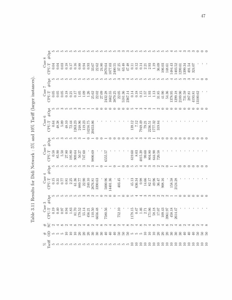
47
Tab
le3.
11R
esult
sfo
rD
idi
Net
wor
k:
5%an
d10
%T
ariff
(lar
ger
inst
ance
s).
%#
#C
ase
3C
ase
4C
ase
5C
ase
6C
ase
7C
ase
8T
ariff
OD
SC
CP
U-T
#O
pt
CP
U-T
#O
pt
CP
U-T
#O
pt
CP
U-T
#O
pt
CP
U-T
#O
pt
CP
U-T
#O
pt
55
20.
195
0.15
50.
585
0.64
50.
055
0.04
55
54
0.40
50.
315
85.9
05
48.3
85
0.05
50.
045
55
80.
975
0.77
55.
503
5.09
30.
055
0.03
55
102
0.94
50.
815
27.8
05
48.1
05
0.18
50.
185
510
41.
835
2.25
519
5.80
572
.44
50.
215
0.17
55
108
81.7
05
61.3
65
909.
643
1263
.23
30.
175
0.16
55
202
179.
525
889.
775
50.2
73
248.
963
1.05
50.
885
520
455
.14
322
.90
374
7.60
111
9.23
11.
095
0.94
55
208
456.
213
240.
102
-0
1421
6.75
11.
265
0.93
55
302
110.
502
2676
.81
398
90.6
91
2045
3.06
125
.62
533
.67
55
304
6656
.48
133
90.6
31
-0
-0
22.0
25
22.6
25
530
8-
0-
0-
0-
027
.09
524
.80
55
402
7580
.56
250
00.9
61
6555
.57
1-
024
32.2
85
2870
.64
55
404
-0
1440
1.36
1-
0-
016
62.5
55
1877
.03
55
408
-0
-0
-0
-0
3879
.25
524
00.5
55
550
275
2.10
140
3.45
1-
0-
022
.05
337
.25
35
504
-0
-0
-0
-0
5181
.36
463
.48
35
508
-0
-0
-0
-0
2367
.14
447
.48
310
52
1178
.15
545
.13
561
9.60
513
9.12
50.
145
0.11
510
54
0.47
463
6.34
58.
034
7.12
40.
185
0.12
510
58
1.46
40.
984
4015
.20
379
49.4
93
0.15
50.
145
1010
22.
713
14.6
64
99.6
04
79.2
14
1.57
52.
215
1010
417
1.06
382
.17
380
4.80
322
36.5
13
1.93
52.
935
1010
858
.18
349
.96
364
4.90
117
77.3
21
1.13
51.
195
1020
217
.07
236
.47
272
0.58
231
9.84
231
.85
536
.09
510
204
109.
432
908.
162
-0
-0
41.9
05
106.
035
1020
839
61.9
72
-0
-0
-0
54.3
65
148.
615
1030
245
8.18
115
8.58
1-
0-
013
78.9
54
1484
.43
410
304
2614
.47
121
24.2
81
-0
-0
1299
.18
514
03.5
25
1030
8-
0-
0-
0-
021
89.9
05
1299
.01
410
402
-0
-0
-0
-0
731.
593
1399
.34
310
404
-0
-0
-0
-0
287.
813
491.
543
1040
8-
0-
0-
0-
041
93.8
14
324.
073
1050
2-
0-
0-
0-
013
100.
621
-0
1050
4-
0-
0-
0-
0-
0-
010
508
-0
-0
-0
-0
-0
-0

48
Tab
le3.
12R
esult
sfo
rD
idi
Net
wor
k:
15%
and
20%
Tar
iff(l
arge
rin
stan
ces)
.
%#
#C
ase
3C
ase
4C
ase
5C
ase
6C
ase
7C
ase
8T
ariff
OD
SC
CP
U-T
#O
pt
CP
U-T
#O
pt
CP
U-T
#O
pt
CP
U-T
#O
pt
CP
U-T
#O
pt
CP
U-T
#O
pt
155
21.
114
1.16
478
.18
422
75.3
25
0.44
50.
315
155
410
.73
47.
694
4986
.55
37.
422
0.29
50.
255
155
854
3.31
481
1.75
3-
0-
00.
275
0.22
515
102
338.
474
2150
.81
328
.47
242
,59
23.
125
3.65
515
104
112.
893
2371
.82
329
2.66
110
4.40
13.
885
3.01
515
108
52.8
32
32.9
61
-0
-0
2.91
52.
975
1520
235
.67
295
2.47
2-
0-
034
4.71
576
1.94
515
204
274.
501
-0
-0
-0
144.
295
156.
794
1520
867
26.4
01
-0
-0
-0
149.
535
2274
.63
515
302
-0
-0
-0
-0
920.
714
4924
.55
315
304
-0
-0
-0
-0
458.
903
51.8
22
1530
8-
0-
0-
0-
013
1.29
372
2.94
315
402
-0
-0
-0
-0
6780
.25
378
3.33
115
404
-0
-0
-0
-0
476.
672
5789
.84
215
408
-0
-0
-0
-0
4535
.04
365
80.8
42
1550
2-
0-
0-
0-
021
551.
691
-0
1550
4-
0-
0-
0-
015
065.
391
-0
1550
8-
0-
0-
0-
0-
0-
020
52
8.00
545
.47
542
.40
418
9.17
30.
225
0.26
520
54
1.45
378
.15
314
0.49
122
09.5
41
0.22
50.
245
205
88.
833
9.79
1-
0-
00.
225
0.29
520
102
1027
.07
511
.28
212
31.8
92
9706
.06
27.
545
7.74
420
104
446.
973
5.30
119
56.5
31
1913
.78
13.
985
3165
.36
520
108
-0
-0
-0
-0
4.61
53.
694
2020
245
4.37
117
44.7
61
-0
-0
1205
.51
433
16.9
14
2020
4-
0-
0-
0-
083
.10
425
.95
320
208
-0
-0
-0
-0
233.
104
23.5
83
2030
2-
0-
0-
0-
063
11.7
53
1853
.35
220
304
-0
-0
-0
-0
4147
.70
329
58.0
72
2030
8-
0-
0-
0-
056
95.3
73
2225
.56
220
402
-0
-0
-0
-0
4714
.99
164
97.5
51
2040
4-
0-
0-
0-
012
304.
761
1965
8.04
120
408
-0
-0
-0
-0
1373
3.04
156
39.2
61
2050
2-
0-
0-
0-
0-
0-
020
504
-0
-0
-0
-0
-0
-0
2050
8-
0-
0-
0-
0-
0-
0

49
3.7 Conclusion and Future Work
In this paper, we have analyzed a two-stage stochastic bilevel pricing problem and its refor-
mulation as a single-stage SBP, focusing on sensitivity analysis with respect to the constraints
linking the tariffs at the two stages of the stochastic program. Several avenues for future re-
search are open. They include the theoretical analysis of the situation involving continuous
random variables, together with the development of a suitable numerical approach that takes
advantage of the network structure, and does not simply relies on a straightforward extension
of techniques developed in the deterministic case. On the modelling side, the extension of the
model to an arbitrary number of stages, either in closed loop or open loop (“feedback Sta-
ckelberg”) poses formidable challenges, both from the theoretical and computational points
of view, and requires investigation.

50
Appendix
Appendix A : Example 2 revisited
Let us consider a two-commodity extension of the network depicted in Figure 3.4 where
origin-destination pairs a−c and d−f are endowed with respective demands n1 = 8 and n2 =
5. Table 3.13 lists each random market price d′j (j = 1, ..., 8) and random demand n′k (k =
1, 2). These are generated according to discrete uniform distributions [dj(1− τ), dj(1 + τ)]
and[nk(1− η), nk(1 + η)
], respectively. Note that the first outcome represents the most
favorable case with respect to the parameters τ and η, and the fourth outcome the least
favorable.
Table 3.13 Random market prices and demands.
SC PROB τ η d′ab d′ac d′ad d′cf d′db d′df d′eb d′ef n′ac n′df
1 0.20 0.10 0.20 3.00 9.10 4.80 1.90 3.30 14.00 1.10 12.80 8 5
2 0.30 0.25 0.30 2.40 10.60 4.00 1.50 2.60 11.90 1.10 14.70 7 5
3 0.30 0.25 0.30 3.40 8.60 5.40 1.80 2.70 11.60 1.10 10.40 9 4
4 0.20 0.40 0.40 4.00 6.30 6.80 2.30 1.80 18.20 0.90 16.40 11 7
Table 3.14 lists paths for the first and second commodities (a − c and d − f) associated
with the second example network (Figure 3.4).

51
Table 3.14 Available paths for commodities a− c and d− f .
OD PATH OD PATH
a− c ρ11 : a− c d− f ρ2
1 : d− b− c− f
ρ12 : a− b− c ρ2
2 : d− e− b− c− f
ρ13 : a− e− b− c ρ2
3 : d− e− f
ρ14 : a− d− b− c ρ2
4 : d− f
ρ15 : a− d− e− b− c

52
3.7.1 Results under the AR case
Tables 3.15–3.16 provide the stochastic and expected optimal solutions under the AR
case, for both unconstrained or nonnegative tariffs. In tables 3.15, 3.16, 3.19, and 3.20, la-
bel ‘EV’ refers to the expected revenue corresponding to four scenarios. The values of the
stochastic solutions are 23.85 and 22.27, respectively, and show that the added cost of sol-
ving the stochastic model is reasonable. It can also be observed from Tables 3.16 and 3.16
that, somewhat counterintuitively, a larger revenue can be obtained by restricting oneself to
nonnegative tariffs, when stochasticity is ignored.
Table 3.15 RP solution under the AR case : unrestricted/nonnegative tariffs.
SC OD Tariff REV EV
STAGE I a− c ρ13 (0.25, 6.60, 1.40) 94.80
d− f ρ22
STAGE II 1 a− c ρ13 (0.30, 6.70, 1.60) 97.50
d− f ρ22
2 a− c ρ13 (0.50, 6.70, 1.50) 91.40
d− f ρ22
3 a− c ρ13 (0.00, 6.50, 1.20) 89.30
d− f ρ22
4 a− c ρ11 (0.00, 6.70, 1.20) 46.90
d− f ρ21
83.09
Total REV (STAGE I+STAGE II) = 177.89

53
Tab
le3.
16E
EV
solu
tion
under
the
AR
case
Unre
stri
cted
tari
ffs
Non
neg
ativ
eta
riff
s
SC
OD
Tar
iffR
EV
EV
Tar
iffR
EV
EV
ST
AG
EI
a−c
ρ1 3
(−0.
87,8.0
0,1.
75)
105.
79
d−f
ρ2 2
ρ1 3
(0.2
5,6.
88,1.7
5)10
0.22
ρ2 2
ST
AG
EII
1a−c
ρ1 3
(−1.
05,8.0
5,1.
95)
106.
00
d−f
ρ2 2
2a−c
ρ1 3
(−0.
62,8.1
0,1.
55)
52.3
6
d−f
ρ2 4
3a−c
ρ1 1
(−1.
12,7.9
0,1.
95)
0.00
d−f
ρ2 4
4a−c
ρ1 1
(−0.
62,8.1
0,1.
55)
56.7
0
d−f
ρ2 1
48.2
5
ρ1 3
(0.0
2,6.
98,1.9
5)10
0.65
ρ2 2
ρ1 3
(0.5
0,6.
80,1.5
5)85.0
1
ρ2 1
ρ1 1
(0.0
0,6.
78,1.5
5)0.
00
ρ2 4
ρ1 1
(0.0
0,6.
98,1.5
5)48.8
6
ρ2 1
55.4
0
Tot
alR
EV
(ST
AG
EI+
ST
AG
EII
)=
154.
04T
otal
RE
V(S
TA
GE
I+ST
AG
EII
)=
155.
62

54
Figure 3.6 (A) illustrates the revenue growth under the AR case, as δ increases, with
Figure 3.6 (B) zooming in on the interval [0, 1]. Table 3.17 displays the optimal tariffs,
second-stage revenue, and total revenue for different values of δ under the AR case.
0 2 4 6 8 10165
180
195
210
225
δ
Rev
enue
0 0.25 0.5 0.75 1165
180
195
205
δ
(A) (B)
Figure 3.6 Sensitivity with respect to δ : (A) The AR case (B) Zoom in.

55
Table 3.17 Revenue and tariff changes for different values of δ under the AR case.
δ Tariff Q REV
[0.00, 0.125] (δ, 6.50 + δ, 1.20 + δ) 79.19 + 27.60δ 169.69 + 53.60δ
[0.125, 0.15] (δ, 6.50 + δ, 1.20 + δ) 79.99 + 21.20δ 170.49 + 47.20δ
[0.15, 0.25] (δ, 6.50 + δ, 1.20 + δ) 80.89 + 15.20δ 171.39 + 41.20δ
[0.25, 0.30] (δ, 6.50 + δ, 1.20 + δ) 81.39 + 13.20δ 171.89 + 39.20δ
[0.30, 0.428] (δ, 6.50 + δ, 1.20 + δ) 82.65 + 9.00δ 173.15 + 35.00δ
[0.428, 0.45] (δ, 6.50 + δ, 0.90 + δ) 82.35 + 13.20δ 171.35 + 39.20δ
[0.45, 0.55] (δ, 6.50 + δ, 0.90 + δ) 84.24 + 9.00δ 173.24 + 35.00δ
[0.55, 0.636] (δ, 6.50 + δ, 0.90 + δ) 86.55 + 4.80δ 175.55 + 30.80δ
[0.636, 0.65] (δ, 6.50 + δ, 1.20 + δ) 83.65 + 7.00δ 174.15 + 33.00δ
[0.65, 0.75] (δ, 6.50 + δ, 1.20 + δ) 86.38 + 2.80δ 176.88 + 28.80δ
[0.75, 0.80] (1.50− δ, 6.50 + δ, 1.20 + δ) 84.88 + 4.80δ 187.38 + 14.80δ
[0.80, 0.13] (1.50− δ, 6.50 + δ, 2) 83.20 + 6.90δ 189.70 + 11.90δ
[0.13, 1.11] (1.50− δ, 6.50 + δ, 1.20 + δ) 86.35 + 4.80δ 187.35 + 14.80δ
[1.11, 1.15] (1.50− δ, 6.50 + δ, 2.00) 86.35 + 4.80δ 192.85 + 9.80δ
[1.15, 1.45] (1.50− δ, 6.50 + δ, 2.00) 88.65 + 2.80δ 195.15 + 7.80δ
[1.45, 1.50] (−2.10 + δ, 6.50 + δ, 2.00) 98.33 176.03 + 21.00δ
[1.50, 1.80] (−3.60 + 2δ, 8.00, 2.00) 100.43− 1.40δ 185.63 + 14.60δ
[1.80, 7.80] (0.00, 8.00, 2.00) 95.39 + 1.40δ 209.39 + 1.40δ
δ ≥ 7.80 (0.00, 8.00, 2.00) 106.31 220.31

56
Table 3.18 Optimal paths for different values of δ under the AR case.
SC OD δ ∈ [0.00, 0.13] δ ∈ [0.13, 1.45] δ ∈ [1.45,∞)
STAGE I a− c ρ13 ρ1
3 ρ13
d− f ρ22 ρ2
2 ρ22
STAGE II 1 a− c ρ13 ρ1
3 ρ13
d− f ρ22 ρ2
2 ρ22
2 a− c ρ13 ρ1
3 ρ13
d− f ρ22 ρ2
2 ρ22
3 a− c ρ13 ρ1
3 ρ13
d− f ρ22 ρ2
2 ρ22
4 a− c ρ11 ρ1
1 ρ13
d− f ρ21 ρ2
2 ρ21

57
3.7.2 Results under the PR case
Tables 3.19–3.20 provide the stochastic and expected optimal solutions under the PR case.
However according to the inequality RP ≥ EEV, the value of the stochastic solution shows
the expected benefit obtained by solving the stochastic model instead of its deterministic
counterpart. As observed earlier, restriction to nonnegative tariffs can actually yield higher
revenues, when stochasticity is ignored (see Tables 3.19 and 3.20).
Table 3.19 RP solution under the PR case : unrestricted/nonnegative tariffs.
SC OD Tariff REV EV
STAGE I a− c ρ13 (0.40,6.89,1.87) 102.13
d− f ρ22
STAGE II 1 a− c ρ13 (0.30, 6.70, 2.20) 100.50
d− f ρ22
2 a− c ρ13 (0.50, 6.80, 1.50) 92.60
d− f ρ22
3 a− c ρ13 (0.30, 6.20, 1.50) 89.30
d− f ρ22
4 a− c ρ11 (0.30, 7.58, 1.50) 53.04
d− f ρ21
85.28
Total REV (STAGE I+STAGE II) = 187.41

58
Tab
le3.
20E
EV
solu
tion
under
the
PR
case
Unre
stri
cted
tari
ffs
Non
neg
ativ
eta
riff
s
SC
OD
Tar
iffR
EV
EV
Tar
iffR
EV
EV
ST
AG
EI
a−c
ρ1 3
(−0.
33,8.0
0,1.
93)
111.
01
d−f
ρ2 2
ρ1 3
(0.0
0,7.
53,1.9
3)10
7.62
ρ2 2
ST
AG
EII
1a−c
ρ1 3
(−0.
42,7.4
2,2.
20)
104.
10
d−f
ρ2 2
2a−c
ρ1 3
(−0.
25,8.7
5,1.
55)
59.5
0
d−f
ρ2 4
3a−c
ρ1 1
(−0.
42,7.2
0,1.
55)
0.00
d−f
ρ2 4
4a−c
ρ1 1
(−0.
42,8.8
0,1.
55)
61.6
0
d−f
ρ2 1
50.9
9
ρ1 3
(0.0
0,7.
00,2.2
0)10
2.00
ρ2 2
ρ1 3
(0.0
0,6.
80,1.5
5)81.6
0
ρ2 4
ρ1 1
(0.0
0,6.
78,1.5
5)0.
00
ρ2 4
ρ1 1
(0.0
0,8.
28,1.5
5)58.0
0
ρ2 1
56.4
8
Tot
alR
EV
(ST
AG
EI+
ST
AG
EII
)=
162.
00T
otal
RE
V(S
TA
GE
I+ST
AG
EII
)=
164.
10

59
Figure 3.7 (A) presents the revenue for different values of δ under the PR case. Figure
3.7 (B) zooms in on the interval [0, 8].
0 2 4 6 8160
180
200
220
δ0 80 160 240
160
175
190
205
220
235
δ
Rev
enue
(B)(A)
Figure 3.7 Sensitivity with respect to δ : (A) The PR case (B) Zoom in.
For simple examples, it is possible to obtain closed form expressions for the revenue,
expressed as a function of the key parameter δ. This is achived in Table 3.21 for the PR case.
Nonuniqueness of the lower level paths can be observed at the critical points corresponding
to δ-values such as δ = 0.462, 2.88 or 8.80.

60
Table 3.21 Revenue and tariff changes for different values of δ under the PR case.
δ Tariff Q REV
[0.00, 0.03] (0, 6.501−δ ,
1.201−δ )
79.19+25.61δ1−δ
169.69+25.61δ1−δ
[0.03, 0.05] (0, 6.501−δ ,
1.201−δ ) 82.43 ↑ 83.73 175.73 ↑ 17.89
[0.05, 0.18] (0, 6.501−δ ,
1.201−δ )
82.65−62.05δ1−δ
173.15−62.05δ1−δ
[0.18, 0.23] (0, 7.92 ↑ 8, 1.46 ↑ 1.94) 87.17 ↑ 86.88 197.53 ↑ 200.62
[0.23, 0.25] (0, 8, 1.501−δ ) 84.31 + 11.2δ 180.81−177.11δ−11.2δ2
1−δ
[0.25, 0.36] (0, 8, 2) 81.91 + 20.8δ 195.91 + 20.80δ
[0.36, 0.37] (0, 8, 2) 73.48 + 44.2δ 187.486 + 44.2δ
[0.37, 0.38] (0, 8, 2) 86.8 + 8.2δ 200.806 + 8.2δ
[0.38, 0.462] (0, 8, 2) 84.07 + 15.4δ 198.07 + 15.4δ
[0.462, 0.525] (0,8,0.901−δ ) 87.64 + 11.20δ 196.14−180.44δ−11.2δ2
1−δ
[0.525, 0.55] (0,8,0.901−δ ) 93.52 202.02−197.52δ
1−δ
[0.55, 1.10] (0, 8, 2) 91.21 + 4.20δ 205.21 + 4.2δ
[1.10, 2.88] (0, 8, 2) 95.83 209.83
[2.88, 4.71] (−1, 9, 3) 96.79 + 1.40δ 205.79 + 1.4δ
[4.71, 6.80] (−7.801+δ
, 9.00, 3.00) 106.31 160.91+223.31δ1+δ
[6.80, 8.80] (−1.00, 9.00, 3.00) 106.31 215.31
δ ≥ 8.80 (− 7.81−δ , 8 + 7.80
1−δ , 2) 106.31 259.31−220.31δ1−δ
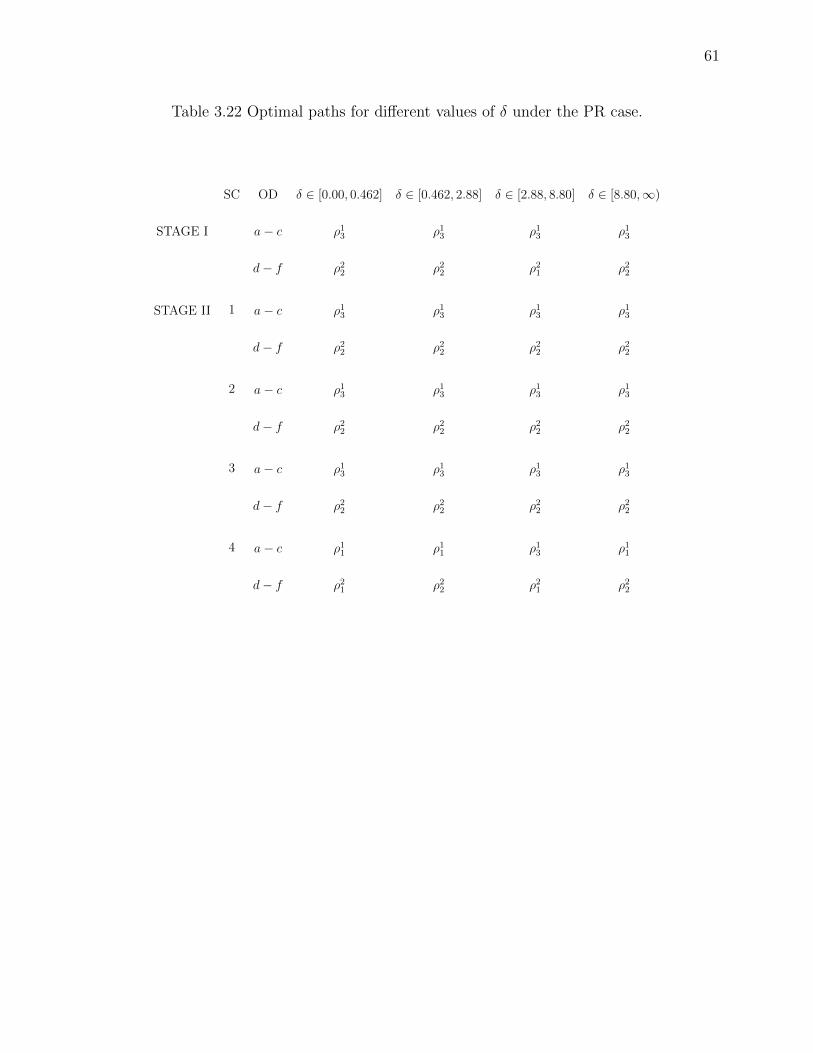
61
Table 3.22 Optimal paths for different values of δ under the PR case.
SC OD δ ∈ [0.00, 0.462] δ ∈ [0.462, 2.88] δ ∈ [2.88, 8.80] δ ∈ [8.80,∞)
STAGE I a− c ρ13 ρ1
3 ρ13 ρ1
3
d− f ρ22 ρ2
2 ρ21 ρ2
2
STAGE II 1 a− c ρ13 ρ1
3 ρ13 ρ1
3
d− f ρ22 ρ2
2 ρ22 ρ2
2
2 a− c ρ13 ρ1
3 ρ13 ρ1
3
d− f ρ22 ρ2
2 ρ22 ρ2
2
3 a− c ρ13 ρ1
3 ρ13 ρ1
3
d− f ρ22 ρ2
2 ρ22 ρ2
2
4 a− c ρ11 ρ1
1 ρ13 ρ1
1
d− f ρ21 ρ2
2 ρ21 ρ2
2

62
CHAPITRE 4
STOCHASTIC NETWORK PRICING : A THEME AND THREE
VARIATIONS
RESUME
Dans cet article, nous poursuivons l’etude de la tarification biniveau stochastique sur deux
etapes (ou periode) introduite dans Alizadeh et al. (2012), ou les peages doivent etre de-
termines sur un sous-ensemble d’arcs du reseau dans le but de maximiser les profits. Nous
considerons trois variations. Dans la premiere variation, nous supposons que la desutilite des
navetteurs integre le delai et les conditions de fiabilite. Dans la seconde variation, nous in-
troduisons des contraintes aleatoires au niveau du meneur dont la pertinence se justifie par
des applications au domaine du transport ou des telecommunications. Dans la troisieme va-
riation du modele, nous integrons la congestion associee aux capacites aleatoires sur les arcs
du reseau. Enfin pour chaque modele, nous proposons une formulation en programmation
mathematique et presentons quelques resultats numeriques.

63
Stochastic network pricing and three variations
Shahrouz Mirza Alizadeh, Patrice Marcotte and Gilles Savard
ABSTRACT
Pursuing on the theme of two-stage bilevel stochastic pricing introduced in Alizadeh et al.
(2012), where profit-maximizing tariffs must be determined on a subset of arcs of a trans-
portation network, we consider three variations. In the first one, it is assumed that the
disutility of commuters incorporates tardiness and reliability terms. The second variation
involves chance constraints at the leader level, and is relevant to the realm of transporta-
tion/telecommunication. The third model embeds congestion associated with random capa-
cities along the arcs of the transportation network. For each model, we provide a mathematical
programming formulation, and illustrate their features through numerical examples.
Key words : Pricing, Bilevel Programming, Stochastic Programming, Mixed Integer Pro-
gramming
Submitted to : EURO Journal on Transportation and Logistics (EJTL) on November 8, 2012

64
4.1 Introduction
In competitive markets, service providers must cope with different aspects of uncertainty
or risk, some of them related to an imperfect knowledge of demand, or of their competitors’
policies. With respect to demand, a firm would like to base a pricing policy on the sensi-
tivity of its potential customers to service delay or service reliability, taking into account
the time-varying and game-theoretic issues that impact the decision process. In recent years,
researchers have realized that this process fits the bilevel programming paradigm, whereby
a ‘leader’ firm takes explicitly into account the rational reaction of customers within its
optimization framework.
Our starting point is the pricing model of Labbe et al. (1998), where profit-maximizing
tariffs have to be set on a prescribed subset of arcs of a multicommodity transportation
network, knowing that demand is assigned to shortest paths with respect to the sum of
initial costs and tariffs. In a series of ensuing works, this modeling approach was adapted
by Bouhtou et al. (2002), Altman and Wynter (2004), Bouhtou et al. (2006), and Bouhtou
et al. (2007a) to the pricing of telecommunication networks, and by Shouping and Baozhuang
(2007) and Gao et al. (2011) in the realm of supply chains.
While the above mentioned studies took place in a deterministic setting, stochastic bilevel
programs have been the topic of articles by Patriksson and Wynter (1997), Christiansen et al.
(2001), Wynter et al. (2002), and Werner (2005), with respective applications in structural
optimization, network planning, and telecommunications. Also relevant to our study is the
work of Audestad et al. (2006), who applied the stochastic programming paradigm to the
analysis of competitive telecommunication markets. More precisely, the authors analyze a
game that takes place between several agents, namely the owner of the network, the custo-
mers, and virtual operators who lease capacity from the network owner, with the objective
of maximizing the joint profit of the market owner and the virtual operators, under either a
deterministic or stochastic setting. One can also mention Kosuch et al. (2012), who consider

65
the problem of simultaneously determining product prices, together with capacities that arise
as stochastic right-hand-sides of multiknapsack constraints, and where chance constraints are
applied to each capacity. The role of the lower level is to enforce the purchase of cheapest
products.
More recently, Alizadeh et al. (2012) introduced a two-stage stochastic model for network
pricing, where each stage is endowed with a bilevel structure. In this model, second-stage
costs and demands may be random, and constraints link the price levels at both stages of the
program. They develop mathematical properties of the model, and provide a reformulation
as a standard bilevel program that can be numerically addressed by ‘standard’ techniques.
In the telecommunication industry, the pricing issue must be addressed by network opera-
tors who offer end-to-end services, while facing competition, uncertainty, risk averse clients,
and other quality of service (QoS) concerns. In this realm, customers select a QoS that best
suits their needs with respect to delay (related to congestion), reliability, costs, or other re-
levant metrics. Since the trade-off values of each customer with respect to these features, or
even the measure of these features themselves, cannot be evaluated with great accuracy, it is
natural to cast the pricing problem within a stochastic framework. Besides, a traditional and
large source of randomness is demand for each service per se. Therefore, stochastic optimiza-
tion is relevant to a large variety of telecommunication network problems, especially at the
design, planning and support levels. The interested reader is referred to Gaivoronski (2005),
who illustrates the power of stochastic programming tools for addressing problems that arise
in the telecommunication industry at the technological, network and enterprise levels.
Motivated by the above-mentioned frameworks of application, the present work focuses
on three stochastic variations on the network pricing theme, each one embedding aspects
that are relevant to real-life applications in transportation or telecommunications. These
incorporate features such as link capacity, path delay, punctuality, and network reliability.
Throughout, we assume that delays are random and that links may become unavailable, due
to congestion or random connection failures. For each model, we specify how randomness

66
enters the mathematical formulation, and provide numerical illustrations based on mixed
integer linear reformulations of the original bilevel programs.
The structure of the paper is as follows. The first section introduces a two-stage stochastic
bilevel model, and more specifically its pricing version. Each of the following three sections
is devoted to one variation, including its formulation and a numerical illustration. The first
variation deals with stochastic disutilities that involve a tardiness term on top of the actual
travel delay, as arises in daily commuting from home to work. The second variation addresses
delay and reliability issues, two features that are common in transportation/telecom networks.
In this model, tardiness enters the leader’s objective through a penalty term, while chance
constraints are used to restrict overcapacity. The third variation, which mostly applies to road
networks, explicitly considers congestion, through the introduction of volume-delay curves.
Following a conclusion, and in order not to disrupt the presentation, the appendix discusses
very shortly the computational complexity of the problem, provides upper bounds that are
valid for the second and third variations, and mentions a continuity result.
4.2 Stochastic Bilevel programming
Bilevel programming allows the natural modelling of hierarchical situations where a subset
of decision variables is not under the direct control of the main optimizer (leader, or upper
level) but is controlled by a follower (user, or lower level) who optimizes its own objective
function with respect to parameters set by the leader. Mathematically, it is expressed as
maxx,y
F1(x, y)
s.t. G1(x, y) ≤ 0,
y ∈ arg miny
f1(x, y),
s.t. g1(x, y) ≤ 0.
(4.1)

67
In the sequel, and in order to simplify the notation, we will only specify the programs of the
leader and the follower, since they contain all the information relevant to the bilevel program.
We now introduce the stochastic bilevel programming (SBP) frameworks that will be used
to formulate the three variations. The first one involves random parameters at the follower
level, while the leader’s objective function involves an expectation. As a general rule, we
use the ‘prime’ notation to indicate the actual value of random variable associated with an
outcome ω. This yields :
maxx
Eξ [F1(x, y′(ξ))]
s.t. G1(x, y′(ω)) ≤ 0, ∀ω ∈ Ω,
miny′(ω)
f1(x, y′(ω), ω),
s.t. g1(x, y′(ω), ω) ≤ 0,
∀ω ∈ Ω,
(4.2)
where ξ (ξ : Ω → <r) is a continuous random vector with realizations ξ (ξ = ξ(ω)) in some
probability space (Ω,F , P ), with Ω denoting the set of all random events, and F the set of
all subsets of Ω. In this ‘wait and see’ framework, the follower solves a deterministic program,
while the risk-neutral leader must factor randomness within its optimization process.
The second SBP takes the form of a chance-constrained bilevel program. Such constraints
are introduced as a measure of quality, and also as a means to limit exposure to risk, and
may be embedded either at the upper or lower level, or at both, as formulated below :

68
maxx
F (x, y)
s.t. G1(x, y) ≤ 0,
PrG2(x, ξ) ≥ H(ξ) ≥ α,
miny
f1(x, y),
s.t. g1(x, y) ≤ 0,
Prg2(y, ξ) ≥ h(ξ) ≥ β,
(4.3)
where G2(x, ξ) and g2(y, ξ) are frequently assumed, to be linear functions with respect to
x and y, respectively. The threshold α and β are reliability parameters belonging to (0, 1),
which can also be interpreted as the risk levels deemed acceptable by the decision makers.
Values close to zero correspond to a risky behaviour, and values close to one to a conservative
attitude.
Let us now focus our attention on a multicommodity transportation network built around
a graph G(N,Λ, K) with node set N , arc set Λ, and commodity set K, each commodity k
(origin-destination pair) being endowed with a demand nk. The set Λ is partitioned into the
subsets Λ1 and Λ2 of tariff and tariff-free arcs, respectively. The set of paths available for
commodity k is denoted by Lk, the set of tariff arcs belonging to path ρ by Λρ1, and the set of
paths including at least one tariff arc by Lk1. The bilevel network pricing problem introduced
by Labbe et al. (1998) consists in maximizing the revenue raised from tariffs, knowing that
user flows are assigned to cheapest paths. Since large tariffs will drive users to tariff-free

69
paths, the optimal trade-off is achieved by solving the bilevel mathematical program
maxt,T
∑k∈K
nk∑ρ∈Lk1
Tρrρ
s.t. Tρ =∑a∈Λρ1
ta, ∀k ∈ K, ∀ρ ∈ Lk1,
minr
∑k∈K
nk[ ∑ρ∈Lk1
Tρrρ +∑ρ∈Lk
∑a∈ρ
carρ],
s.t.∑ρ∈Lk
rkρ = 1, ∀k ∈ K,
rρ ≥ 0, ∀k ∈ K, ∀ρ ∈ Lk,
(4.4)
where t is the vector of tariff variables controlled by the leader, T the vector of revenue raised
from the various paths, and c the vector of fixed costs along the arcs. The leader constraint
establishes compatibility between tariffs and revenues, while the follower’s constraints consist
in flow conservation and flow nonnegativity. The proportion of flow from commodity k as-
signed to path ρ is denoted by rkρ , and it has been shown that, without loss of generality,
this variable can be restricted to the values zero or one, i.e., it can be considered as an in-
dicator function, in the absence of capacities. Throughout, we will make the following basic
assumptions :
1. For each commodity, there exists at least one path composed entirely of tariff-free arcs,
and whose availability (probability of being available) is strictly positive.
2. There does not exist a pricing procedure that yields positive returns and simultaneously
generates a negative-cost cycle. This assumption ensures that the lower level flows are
assigned to shortest paths.
3. Competition prices are fixed and are not influenced by the leader’s tariffs.
4. Demand is fixed and can be split between the paths of the network.
Note that the first two assumptions imply that the upper level revenue is bounded from
above. In the following sections, we extend Program (4.4) to the stochastic framework intro-

70
duced at the beginning of this section.
4.3 First variation : Stochastic disutility
In the first variation, we introduce stochastic disutility at the user level. Disutility is mo-
delled as a function of fixed costs, tariffs, tardiness and reliability, and represents a situation
where users are ready to compromise their target arrival time for higher reliability. To achieve
this goal, the disutility terms are expressed as the ratio of tardiness over reliability, both the
numerator and denominator being random.
In this model, darca (ξ) and dnode
j (ξ) denote random delays along the arcs and nodes, respec-
tively, Hk refers to the target time (deadline) to destination D(k) associated with commodity
k, and pk is the penalty associated with one unit of tardiness, the latter being equal to
max
0, gρ(ω)−Hk
(4.5)
where the total random delay along a given path ρ ∈ Lk is given by
gρ(ξ) =∑a∈ρ
darca (ξ) +
∑j∈ρ|j 6=D(k)
dnodej (ξ). (4.6)
As mentioned previously, network links may become unavailable, due to unforeseen fai-
lures. We assume that the leader has perfect knowledge about the state of its own tariff links,
but not those of the competition. In order to model this situation, we introduce an exogenous
measure of the availability ha(ξ) ∈ (0, 1] of a tariff-free link. Assuming independence between
the links, the availability of a path is thus given by
h′ρ(ξ) =∏a∈ρ
ha(ξ) for ∀k ∈ K, ρ ∈ Lk.
The first variation is then expressed as the mathematical program

71
maxt,T
Eξ
[∑k∈K
nk∑ρ∈Lk1
Tρr′ρ(ξ(ω))
]s.t.
∑a∈Λρ1
ta = Tρ, ∀k ∈ K, ∀ρ ∈ Lk1,
minr
∑k∈K
nk∑ρ∈Lk
[(Tρ +
∑a∈ρ
ca + pk max
0, gρ(ω)−Hk
)/h′ρ(ω)]r′ρ(ω),
s.t.∑ρ∈Lk
r′ρ(ω) = 1, ∀k ∈ K,
r′ρ(ω) ≥ 0, ∀k ∈ K,
∀ω ∈ Ω,
(4.7)
where r′ρ(ω) is the indicator variable corresponding to outcome ω, that takes value one if the
flow of commodity k is assigned to path ρ ∈ Lk, and zero otherwise. As mentioned before, the
‘prime’ symbol refers to the actual value of the random variable associated with an outcome
ω. For instance, c′ρ(ω) denotes the fixed cost of path ρ ∈ Lk for any realization ω ∈ Ω, i.e.,
c′ρ(ω) = (∑a∈ρ
ca + pk max
0, gρ(ω)−Hk
)/h′ρ(ω).
In the standard fashion, we rewrite Programs (4.7) as a mixed-integer program. To achieve
this, we introduce a variable ta,ρ(ω) for each path ρ ∈ Lk, tariff arc a ∈ Λ1 and outcome ω ∈ Ω,
which takes value ta if and only if commodity k is assigned to path ρ ∈ Lk going through
tariff arc a, and is equal to zero otherwise. We obtain
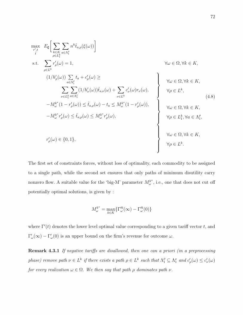
72
maxr′,tt
Eξ
[∑k∈Kρ∈Lk1
∑a∈Λρ1
nk ta,ρ(ξ(ω))
]
s.t.∑ρ∈Lk
r′ρ(ω) = 1, ∀ω ∈ Ω, ∀k ∈ K,
(1/h′ρ(ω))∑a∈Λρ1
ta + c′ρ(ω) ≥∑ν∈Lk1
∑a∈Λν1
(1/h′ν(ω))ta,ν(ω) +∑ν∈Lk
c′ν(ω)rν(ω),
∀ω ∈ Ω,∀k ∈ K,
∀ρ ∈ Lk,
−Mk∗ω (1− r′ρ(ω)) ≤ ta,ρ(ω)− ta ≤Mk∗
ω (1− r′ρ(ω)),
−Mk∗ω r′ρ(ω) ≤ ta,ρ(ω) ≤Mk∗
ω r′ρ(ω),
∀ω ∈ Ω,∀k ∈ K,
∀ρ ∈ Lk1,∀a ∈ Λρ1,
r′ρ(ω) ∈ 0, 1,
∀ω ∈ Ω,∀k ∈ K,
∀ρ ∈ Lk.
(4.8)
The first set of constraints forces, without loss of optimality, each commodity to be assigned
to a single path, while the second set ensures that only paths of minimum disutility carry
nonzero flow. A suitable value for the ‘big-M’ parameter Mk∗ω , i.e., one that does not cut off
potentially optimal solutions, is given by :
Mk∗
ω = maxk∈KΓ′kω (∞)− Γ′kω (0)
where Γ′(t) denotes the lower level optimal value corresponding to a given tariff vector t, and
Γ′ω(∞)− Γ′ω(0) is an upper bound on the firm’s revenue for outcome ω.
Remark 4.3.1 If negative tariffs are disallowed, then one can a priori (in a preprocessing
phase) remove path ν ∈ Lk if there exists a path ρ ∈ Lk such that Λρ1 ⊆ Λν
1 and c′ρ(ω) ≤ c′ν(ω)
for every realization ω ∈ Ω. We then say that path ρ dominates path ν.

73
4.3.1 A numerical example
In this section, we illustrate the model through an example inspired from the airline/telecom
network shown in Figure 4.1, where fixed costs are displayed next to the corresponding arcs.
The demand associated with commodities a − c and d − f is set to n1 = 8 and n2 = 5 res-
pectively, and the available paths for each commodity are displayed in Table 4.1. The vector
of deadlines at destination (target arrival times) is H = (5.5, 6.3), and the vector of unit
tardiness penalties is set to p = (0.2, 0.5). Table 4.2 contains the three distinct sets of fixed
cost data that were considered.
Free arcs
Tariff arcs
ed
a
f
c
1
b
15
12t3
3
3
25
t1
10
1 + t2
Figure 4.1 Example network

74
Table 4.1 Available paths for commodities a− c and d− f
OD PATH OD PATH
a− c ρ11 : a− c d− f ρ2
1 : d− f
ρ12 : a− b− c ρ2
2 : d− e− f
ρ13 : a− e− b− c ρ2
3 : d− e− b− c− f
ρ14 : a− d− b− c ρ2
4 : d− b− c− f
ρ15 : a− d− e− b− c
Table 4.2 Fixed costs along the arcs
# ae bc de ab ac ad cf db df eb ef
1 0 1 0 3 10 5 2 3 15 1 12
2 0 0 0 7 4 4 1 11 32 2 20
3 2 1 1 2 6 2 0 4 15 2 18
In the realm of air transportation, arc and node delays allow the representation of air
travel times and ground delays, respectively. Those can be influenced by weather conditions
or technical problems, among other factors, and have a ripple effect throughout the network.
In the world of telecommunications, arc delays are related to transmission along the lines of
the network, while queueing occurs at the nodes.
Tables 4.3-4.5 list the fixed part of node delays dnodej (j = a, b, c, d, e, f), link de-
lays darca (a ∈ ae, bc, de, ab, ac, ad, cf, db, df, eb, ef), and random link reliabilities of tariff-
free link ha (a ∈ ab, ac, ad, cf, db, df, eb, ef), respectively. These are generated according

75
to discrete uniform distributions[υnodej (1− η), υnode
j (1 + η)], [υarc
a (1− η), υarca (1 + η)], and
[κa(1− η),κa(1 + η)], respectively, where vectors υarc, υnode, and refer to the free flow tra-
vel/transmission time on the arcs and through the nodes, respectively, and κ refers to the
free flow reliability on the arcs. Vectors υarc and υnode are given as
υarc = (5.34, 0.97, 4.46, 1.36, 9.95, 4.63, 1.29, 1.30, 5.78, 2.68, 3.35),
υnode = (0.32, 0.82, 1.28, 0.35, 1.78, 1.41),
and
κ = (0.95, 0.90, 0.75, 0.80, 0.70, 0.90, 0.85, 0.70).
Note that, with respect to the parameter η, the first and fourth outcomes are the most and
least favorable, respectively. Finally, throughout this paper, the abbreviations SC and PROB
will refer to a scenario and its associated reliability.
Table 4.3 Random node delays
SC PROB η dnodea dnode
b dnodec dnode
d dnodee dnode
f
1 0.20 0.10 0.30 0.77 1.20 0.33 1.67 1.33
2 0.30 0.25 0.29 0.74 1.15 0.31 1.60 1.27
3 0.35 0.25 0.30 0.76 1.18 0.32 1.65 1.30
4 0.15 0.40 0.23 0.59 0.92 0.25 1.28 1.02

76
Table 4.4 Random link delays
SC darcae darc
bc darcde darc
ab darcac darc
ad darccf darc
db darcdf darc
eb darcef
1 5.02 0.91 4.19 1.28 9.35 4.35 1.21 1.22 5.43 2.52 3.15
2 4.81 0.87 4.01 1.22 8.95 4.17 1.16 1.17 5.20 2.41 3.01
3 4.94 0.90 4.13 1.26 9.20 4.28 1.19 1.20 5.35 2.48 3.10
4 3.84 0.70 3.21 0.98 7.16 3.33 0.93 0.94 4.16 1.93 2.41
Table 4.5 Random link reliability of tariff-free links
SC hab hac had hcf hdb hdf heb hef
1 0.89 0.85 0.71 0.75 0.66 0.85 0.80 0.66
2 0.85 0.81 0.67 0.72 0.63 0.81 0.77 0.63
3 0.88 0.83 0.69 0.74 0.65 0.83 0.79 0.65
4 0.68 0.65 0.54 0.58 0.50 0.65 0.61 0.50
In order to assess the loss of performance due to neglecting randomness, we will compare
the above revenues with the ones obtained from a deterministic approximation based on the
expected values of the random parameters (EEV). Those are obtained in two phases. First,
we solve the expected value problem corresponding to Program (4.2)

77
maxx
F1(x, y)
s.t. G1(x, y) ≤ 0,
miny
f1(x, y, ω),
s.t. g1(x, y, ω) ≤ 0,
(4.9)
where ω = E[ξ]. Next, letting x denote a first stage optimal solution of Program (4.9), we
define EEV as
max Eξ [F1(x, y′(ξ))]
s.t. G1(x, y′(ω)) ≤ 0, ∀ω ∈ Ω,
miny′(ω)
f1(x, y′(ω), ω),
s.t. g1(x, y′(ω), ω) ≤ 0,
∀ω ∈ Ω.
(4.10)
Tables 4.6 and 4.7 present the stochastic and EEV solutions of Program (4.8), correspon-
ding to the given data and different sets of the fixed costs. The abbreviations OD and REV
refer to commodity and revenue, respectively, and columns ‘I’, ‘II’, ‘III’ and, ‘IV’ refer to the
scenario indices.

78
Table 4.6 Stochastic optimal solutions of Program (4.8)
# OD I II III IV Tariff REV
1 a− c ρ12 ρ1
2 ρ12 ρ1
3 (−0.16, 7.35,−0.76) 58.61
d− f ρ21 ρ2
1 ρ21 ρ2
1
2 a− c ρ13 ρ1
3 ρ13 ρ1
3 (−9.89, 11.32, 4.46) 81.85
d− f ρ23 ρ2
3 ρ23 ρ2
2
3 a− c ρ12 ρ1
2 ρ12 ρ1
2 (−3.32, 3.73,−0.52) 43.48
d− f ρ23 ρ2
3 ρ23 ρ2
1
Table 4.7 EEV optimal solutions of Program (4.8)
# OD I II III IV Tariff REV
1 a− c ρ12 ρ1
2 ρ12 ρ1
3 (−0.21, 7.32,−1.61) 57.10
d− f ρ21 ρ2
1 ρ21 ρ2
2
2 a− c ρ11 ρ1
3 ρ11 ρ1
3 (−4.39, 5.83, 9.91) 29.96
d− f ρ24 ρ2
4 ρ24 ρ2
1
3 a− c ρ12 ρ1
2 ρ12 ρ1
3 (−3.77, 4.10,−0.86) 37.19
d− f ρ23 ρ2
1 ρ23 ρ2
1
From Tables 4.6 and 4.7, we observe that the loss of revenue associated with the determi-
nistic approximation can be in excess of 10%, which confirms the relevance of the stochastic
formulation. Tables 4.8 and 4.9 provide sensitivity information with respect to changes in
tardiness penalty p and deadline H, for the first data set, illustrating how optimal paths

79
vary. A graphical representation of the sensitivity is provided in Figures 4.2 and 4.3.
From an economic standpoint, one expects that higher penalty sensitivity will drive com-
muters to more reliable paths, usually (partially) controlled by the leader, who can then take
advantage of the situation to increase tariffs and revenues (see Figure 4.2). The impact of the
variation of the deadline H is less straightforward. Indeed, increasing H may render attractive
a previously unattractive of even infeasible tariff path, and consequently open new opportu-
nities for increasing tariffs and revenues. This can be observed in the two upper graphs of
Figure 4.3 . Alternatively, large values of H can render attractive a longer tariff-free path,
and then force the leader to lower its tariffs, leading to lower revenue, as can be seen on
the lower graph of Figure 4.3. A priori, and without solving the problem, one cannot predict
which of the two situations will occur.
Table 4.8 Sensitivity analysis with respect to p for the first data set (#1)
p I II III IV
[0.00, 0.02] (ρ13, ρ
23) (ρ1
3, ρ23) (ρ1
3, ρ23) (ρ1
3, ρ21)
[0.02, 0.15] (ρ13, ρ
23) (ρ1
3, ρ23) (ρ1
3, ρ23) (ρ1
3, ρ22)
[0.15, 0.31] (ρ12, ρ
23) (ρ1
2, ρ23) (ρ1
2, ρ23) (ρ1
3, ρ22)
p ≥ 0.31 (ρ12, ρ
21) (ρ1
2, ρ21) (ρ1
2, ρ21) (ρ1
3, ρ21)

80
Table 4.9 Sensitivity analysis with respect to H for the first data set (#1)
H I II III IV
[0.00, 6.30] (ρ12, ρ
21) (ρ1
2, ρ21) (ρ1
2, ρ21) (ρ1
3, ρ21)
[6.30, 6.84] (ρ12, ρ
21) (ρ1
3, ρ21) (ρ1
2, ρ21) (ρ1
3, ρ21)
[6.84, 7.14] (ρ12, ρ
21) (ρ1
3, ρ21) (ρ1
3, ρ21) (ρ1
3, ρ21)
[7.14, 7.47] (ρ13, ρ
21) (ρ1
3, ρ21) (ρ1
3, ρ21) (ρ1
3, ρ21)
[7.47, 8.86] (ρ13, ρ
23) (ρ1
3, ρ23) (ρ1
3, ρ23) (ρ1
3, ρ22)
H ≥ 8.86 (ρ13, ρ
23) (ρ1
3, ρ23) (ρ1
3, ρ23) (ρ1
3, ρ21)
0 0.1 0.2 0.3 0.4 0.560
80
100
Rev
enue
0 1 2 3 440
80
120
0 0.5 1 1.540
60
80
p
#3
#1
#2
Figure 4.2 Sensitivity with respect to the tardiness penalty p

81
0 5 10 1540
80
120
Rev
enue
0 5 10 1570
90
110
0 5 10 1540
50
60
H
#1
#2
#3
Figure 4.3 Sensitivity with respect to the deadline H
4.4 Second variation : Chance constraints
We now introduce the framework of the second variation, which shares several features
with the first one. However, the differences are twofold. First, the tardiness penalty is incurred
by the leader. Second, reliability of an arc is now related to the flow that it carries, and to
a random target capacity. A chance constraint, whose role is to prevent overflow and ensure
a reliable performance level of the system, is then imposed to the leader. In this setting, the
path choice of the follower is not influenced by the reliability of the paths, since the constraint
imposed at the upper level ensures a predetermined and satisfactory level of service.
Notation-wise, the model involves a random vector of link capacities C ′(ξ) (ξ : Ω′ → <|Λ1|)
at the upper level. The role of chance constraints is then to ensure that the probability of not
meeting these target values lies below some predetermined threshold. According to the above
considerations, the corresponding model takes the form of the chance constrained bilevel

82
program
maxt,T
∑k∈K
∑ρ∈Lk1
(Tρ − pkEξ
[max
0, gρ(ξ)−Hk
] )fρ
s.t.∑a∈Λρ1
ta = Tρ, ∀k ∈ K, ∀ρ ∈ Lk1,
xa =∑k∈K
∑ρ∈Lk|a∈ρ
fkρ , ∀a ∈ Λ1,
Prxa ≥ C ′a(ξ) ≤ αa, ∀a ∈ Λ1,
minf
∑k∈K
[ ∑ρ∈Lk1
Tρfkρ +
∑ρ∈Lk
∑a∈ρ
cafkρ
],
s.t.∑ρ∈Lk
fkρ = nk, ∀k ∈ K,
fkρ ≥ 0, ∀k ∈ K, ∀ρ ∈ Lk,
(4.11)
where f is the vector of path flows and gρ(ξ), defined in Equation (4.6), represents the total
delay. The parameter αa specifies the maximum risk of overloading, and may be interpreted
as a ‘protection level’ associated with link a.
According to the form of the chance constraints, setting the value of the tolerance parame-
ter α close to one reflects a risky attitude with respect to reliability requirements, but might
yield high profit. At the other end of the spectrum, setting α close to zero corresponds to a
risk averse leader. It will ensure high reliability (low congestion), at the expense of revenue.
Actually, if α = 0, then no flow at all (except for the case of infinite capacity) can be assigned
to the arcs that are in control of the leader, hence revenue (profit) is null.
In order to deal numerically with chance constraints without resorting to simulation,
the latter being computationally expensive, we make the assumption that arc capacities are
distributed according to uniform variates U [θaCa, Ca], where the parameter θ is an indicator
of the reliability of the link : the higher θa, the higher the probability that the target capacity
Ca be fully available. Low values of θa reflect a situation where disruptions may occur with
high probability, and thus that the link become partially or totally unavailable. Denoting by

83
Fa the cumulative distribution function of U [θaCa, Ca], we can write
Prxa ≥ C ′a(ξ) ≤ αa,
⇐⇒ xa ≤ F−1a (αa),
⇐⇒ xa ≤ (αa + (1− αa)θa)Ca,
and it follows that Program (4.11) can be reformulated as
R(θ) = maxt,T
∑k∈K
∑ρ∈Lk1
(Tρ − pkEξ
[max
0, gρ(ξ(ω))−Hk
] )fρ
s.t.∑a∈Λρ1
ta = Tρ, ∀k ∈ K, ∀ρ ∈ Lk1,
xa =∑k∈K
∑ρ∈Lk|a∈ρ
fkρ , ∀a ∈ Λ1,
xa ≤ (αa + (1− αa)θa)Ca, ∀a ∈ Λ1,
minf
∑k∈K
[ ∑ρ∈Lk1
Tρfρ +∑ρ∈Lk
∑a∈ρ
cafkρ
],
s.t.∑ρ∈Lk
fkρ = nk, ∀k ∈ K,
fkρ ≥ 0, ∀k ∈ K, ∀ρ ∈ Lk.
(4.12)
4.4.1 A numerical example
Let us again consider the network depicted in Figure 4.1, where the relevant information
is left unchanged, together with the additional data
C = (10, 20, 25), θ = (0.15, 0.20, 0.25), α = (0.05, 0.03, 0.04).

84
Table 4.10 Second variation : optimal solutions
# OD Flow Tariff REV
1 a− c (8, 0, 0, 0, 0) (−1, 9, 3) 41.22
d− f (0, 0.52, 0, 4.48)
2 a− c (8, 0, 0, 0, 0) (−15, 17, 9) 107.44
d− f (0, 0.52, 4.48, 0)
3 a− c (8, 0, 0, 0, 0) (−9, 10, 1) 44.80
d− f (0.52, 0, 0, 4.48)
Table 4.10 displays the optimal solutions of Program (4.12) (link flows, tariffs and revenue)
for the three data sets introduced earlier for the first variation. While flow is assigned to a
single path for the OD pair a− c, this is not the case for OD pair d− f , where flow is split
between two paths, in order to meet the capacity requirements set by the leader. Since path
flows at the lower level must be assigned to shortest paths, it follows that all paths that
carry positive flow are of equal and minimal costs. Moreover, since the same values of the
parameters α and θ have been uses across the three data sets, the path flow proportions do
not vary, as can be observed in Table 4.10, where we assumed identical capacities for each
data set. Sensitivity with respect to parameters α and θ is provided, for the first data set,
in Figures 4.4 and 4.5, as well as in Tables 4.11 and 4.12. When sensitivity is performed
with respect to a vector (versus one of its components), it is understood that all components
vary simultaneously and assume a common value. Note that when the parameters α2 and θ2
of tariff arc 2 are set to their initial values, varying the parameters of the two other tariff
arcs does not result in a revenue increase. The reason of this occurrence is because of less
role of the tariff arcs ae and de in the paths that the users are interested. Notwithstanding,
increasing simultaneously the three parameters results in a faster revenue increase.

85
0 0.2 0.4 0.6 0.8 130
50
70
90
110
α
Rev
enue
αα
1, α
3
α2
Figure 4.4 Second variation : sensitivity of revenue with respect to α
0 0.2 0.4 0.6 0.8 10
30
60
90
120
θ
Rev
enue
θθ
1, θ
3
θ2
Figure 4.5 Second variation : sensitivity of revenue with respect to θ

86
Table 4.11 Second variation : sensitivity of revenue with respect to α
α OD Flow REV
[0.000, 0.062] a− c (8, 0, 0, 0, 0) 37.73 + 116.35α
d− f (0, 1− 16α, 0, 4 + 16α)
[0.062, 0.334] a− c (9− 16α, 0,−1 + 16α, 0, 0) 38.02 + 111.69α
d− f (0, 0, 5, 0)
[0.334, 0.764] a− c (6.5− 8.5α, 0, 1.5 + 8.5α, 0, 0) 55.50 + 59.34α
d− f (0, 0, 5, 0)
α ≥ 0.764 a− c (0, 0, 8, 0, 0) 100.85
d− f (0, 0, 5, 0)

87
Table 4.12 Second variation : sensitivity of revenue with respect to θ
θ OD Flow REV
[0.000, 0.078] a− c (8, 0, 0, 0, 0) 7.13 + 216.07θ
d− f (3.4− 43.4θ, 1 + 24θ, 0, 0.6 + 19.4θ)
[0.078, 0.107] a− c (8, 0, 0, 0, 0) 12.93 + 141.73θ
d− f (0, 4.4− 19.4θ, 0, 0.6 + 19.4θ)
[0.107, 0.123] a− c (9.285− 22.25θ, 0,−1.285 + 22.25θ, 0, 0) 13 + 141.08θ
d− f (0, 4.9− 9.9θ, 0, 0.1 + 9.9θ)
[0.123, 0.334] a− c (7.5− 9.5θ, 0, 0.5 + 9.5θ, 0, 0) 13.35 + 138.23θ
d− f (0, 4.9− 9.9θ, 0, 0.1 + 9.9θ)
[0.334, 0.495] a− c (12.4− 19.4θ, 0,−4.4 + 19.4θ, 0, 0) 14.29 + 135.42θ
d− f (0, 0, 5, 0)
[0.495, 0.788] a− c (7.5− 9.5θ, 0, 0.5 + 9.5θ, 0, 0) 48.41 + 66.54θ
d− f (0, 0, 5, 0)
θ ≥ 0.788 a− c (0, 0, 8, 0, 0) 100.85
d− f (0, 0, 5, 0)
Let us focus on the first data set. In Table 4.11, we observe that the lower level solution is
not unique at the critical values 0.062, 0.334, and 0.764 of the parameter α. The same situation
occurs for θ at points 0.078, 0.107, 0.123, 0.334, 0.495, and 0.788 (see Table 4.12). It is
interesting to note that the corresponding sensitivity curves (see Figure 4.4 and Figure 4.5) are
continuous, increasing and piecewise linear, but not necessarily concave, as might have been

88
expected. The two dotted curves, corresponding to fixed values for α2 and θ2, respectively,
illustrate the role played by the second tariff arc bc. Indeed, higher values of the parameter α
relate to an increase in path reliability. Figure 4.6 shows the variation of the revenue function,
jointly in α and θ, where common values of α and θ are shown along the abscissa.
0 0.2 0.4 0.6 0.8 10
40
80
120
α, θ
Rev
enue
α & θαθ
Figure 4.6 Revenue with respect to simultaneous changes in α and θ
We close this section with a depiction of sensitivity analysis with respect to tardiness
and deadline arrival. Since the penalty is incurred on the leader, it is clear that revenue is a
decreasing (actually continuous, piecewise linear and convex) function of p . If tariff links are
the most reliable, large values of p force the leader to reduce its tariffs in order to prevent
the lower level flows to be assigned to less reliable paths. In contrast, revenue increases when
deadline H increases. The ‘max’ operator involved in the tardiness term makes it nonlinear,
but it need not be concave. As H goes beyond some threshold value, it becomes irrelevant,
and revenue stabilizes to some maximum value. This is illustrated in Figure 4.7.

89
0 0.5 1 1.540
42
44
46
p
Rev
enue
0 5 10 1525
30
35
40
45
50
H
Figure 4.7 Sensitivity with respect to tardiness penalty p and deadline H
4.5 Third variation : Congestion
Congestion is a prevalent issue in urban transportation (road works, weather conditions,
excess demand), as well as in telecommunications (traffic, network degradation), where it
is directly related to the ‘quality of service’. In contrast with the second variation, where
quality of service was enforced through a chance constraint, the third variation explicitly
models congestion via a volume-delay function of the BPR (Bureau of Public Roads) type :
υarca
[1 +
(xa
C ′a(ξ)
)m]where, for every link a, υarc
a denotes the ‘free-flow’ travel time, xa the flow along link a, C ′a(ξ)
the random capacity of the link, and m is an exponent frequently set to the value 4. Assuming
a value of one for the value-of-time parameter that converts delays into monetary units, the

90
travel delay on path ρ takes the form
gρ(x, ξ) =∑a∈Λρ1
υarca
[1 +
( xaC ′a(ξ)
)m]+∑a∈Λρ2
υarca
=∑a∈Λρ1
υarca (
xaC ′a(ξ)
)m +∑a∈Λρ
υarca . (4.13)
Assuming that customers only integrate costs (not congestion) within their objective leads
to the following bilevel formulation of the stochastic pricing problem over a network :
maxt,T
∑k∈K
∑ρ∈Lk1
Tρfρ
s.t.∑a∈Λρ1
ta = Tρ, ∀k ∈ K, ∀ρ ∈ Lk1,
Prgρ(x, ξ) ≤ Hk ≥ βk, ∀k ∈ K, ∀ρ ∈ Lk1,
xa =∑k∈K
∑ρ∈Lk|a∈ρ
fρ, ∀a ∈ Λ1,
minf
∑k∈K
[ ∑ρ∈Lk1
Tρfρ +∑ρ∈Lk
∑a∈ρ
cafρ],
s.t.∑ρ∈Lk
fρ = nk, ∀k ∈ K,
fρ ≥ 0, ∀k ∈ K, ∀ρ ∈ Lk,
(4.14)
where the leader’s chance constraints guarantee that travel time on the paths involving at
least one tariff arc respect to the target time, with some tolerance to tardiness βk that
depends on the commodity index k. Such requirement can be satisfied by attracting flow to
the reliable paths in control of the leader, striking the right balance between low tariffs (that
attract flow), and tariffs sufficiently large to prevent high congestion levels that would lead
to violations of the chance constraints.
In the model, we assume that the capacity of link a is distributed according to a discrete
uniform random variable over the interval [θC,C]. Since the number of outcomes is finite,
it is then possible to replace the chance constraints by linear constraints. To this aim, we

91
introduce the auxiliary binary variables uρ(ω) for each ω ∈ Ω′, which is equal to 0 if and only
if gρ(x, ω) ≤ Hk, together with a ‘big-M’ constant M . One can then enforce the tardiness
constraints, for every commodity k, through the inequalities
gρ(x, ω)−Muρ(ω) ≤ Hk, (4.15)
Eξ [uρ(ω)] ≤ 1− βk. (4.16)
This yields the mixed integer nonlinear bilevel program
maxu,t,T
∑k∈K
∑ρ∈Lk1
Tρfρ
s.t. xa =∑k∈K
∑ρ∈Lk|a∈ρ
fρ, ∀a ∈ Λ1,
∑a∈Λρ1
ta = Tρ,
Eξ [uρ(ξ(ω))] ≤ 1− βk,
∀k ∈ K, ∀ρ ∈ Lk1,
gρ(x, ω)−Muρ(ω) ≤ Hk,
uρ(ω) ∈ 0, 1,
∀k ∈ K, ∀ρ ∈ Lk1, ∀ω ∈ Ω′,
minf
∑k∈K
[ ∑ρ∈Lk1
Tρfρ +∑ρ∈Lk
∑a∈ρ
cafρ],
s.t.∑ρ∈Lk
fρ = nk, ∀k ∈ K,
fρ ≥ 0, ∀k ∈ K, ∀ρ ∈ Lk.
(4.17)
In order to address Program (4.17) numerically, we replace the convex and link-separable
functions gρ by piecewise linear lower approximations over the intervals [0, (UBa)m], where
the upper bound UBa is set to
UBa =∑k∈K
∑ρ∈Lk|a∈ρ
nk

92
for each a ∈ Λ1. This leads to the linear constraints
Xa ≥ qsaxa + wsa,
where qsa and wsa are the coefficients of the tangent line to the function (xa)m at the point xsa,
that is, qsa = m(xsa)m−1 and wsa = (1 −m)(xsa)
m for a ∈ Λ1 and s = 1, ..., Sa. It follows from
the convexity of gρ that this approximation is valid, i.e., it yields points (xa, Xa) that lie on
the graph and not strictly above the approximating curve (xa, Xa), at optimality. This leads
to the mixed integer program
maxt,T
∑k∈K
∑ρ∈Lk1
Tρfρ
s.t. Xa ≥ qsaxa + wsa, ∀a ∈ Λ1, s = 1, .., Sa,
xa =∑k∈K
∑ρ∈Lk|a∈ρ
fρ,
Xa ≤ (UBa)m,
∀a ∈ Λ1,
∑a∈Λρ1
ta = Tρ,
Eξ [uρ(ξ(ω))] ≤ 1− βk,
∀k ∈ K, ∀ρ ∈ Lk1,
∑a∈Λρ1
Va(ω)Xa −Muρ(ω) ≤ Hk,
uρ(ω) ∈ 0, 1,
∀k ∈ K, ∀ρ ∈ Lk1,
∀ω ∈ Ω′,
minf
∑k∈K
[ ∑ρ∈Lk1
Tρfρ +∑ρ∈Lk
∑a∈ρ
cafρ],
s.t.∑ρ∈Lk
fρ = nk, ∀k ∈ K,
fρ ≥ 0, ∀k ∈ K, ∀ρ ∈ Lk,
(4.18)

93
where
Va(ω) = υarca /(C ′a(ω)
)m.
Program (4.18) can be solved through an iterative procedure based on iteratively refining
the approximation of gρ. The algorithm is stopped as soon as the difference between to
consecutive values of the objective is less than some predetermined threshold ε. Note that,
at each iteration, the mixed integer approximation yields an upper bound on the actual
revenue. Symmetrically, a piecewise linear over-approximation of the BPR curves, yielding
an interpolation based on cords of the original power function, would have yielded a lower
bound on the actual revenue. In both cases, the iterative solutions converge to the solution of
the original solution, as the width of the subintervals involved in the partition tend to zero.
4.5.1 A numerical example
Let us consider the network and data used for the second variation. The vectors H and β
are set to (15, 11) and (0.90, 0.85), respectively, while the BPR exponent is set to 2 (quadratic
volume-delay curve). Ten outcomes of random link capacities C ′a(ξ) are generated according
to a uniform distribution [θCa, Ca], with associated probability vector
(0.05, 0.04, 0.10, 0.15, 0.01, 0.20, 0.15, 0.05, 0.10, 0.15).
Table 4.13 displays the optimal solutions of Program (4.18) for the three data sets.
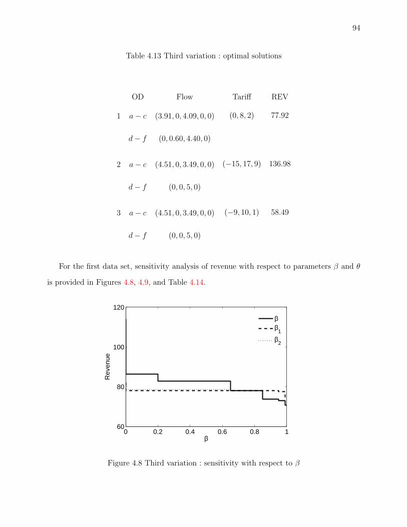
94
Table 4.13 Third variation : optimal solutions
OD Flow Tariff REV
1 a− c (3.91, 0, 4.09, 0, 0) (0, 8, 2) 77.92
d− f (0, 0.60, 4.40, 0)
2 a− c (4.51, 0, 3.49, 0, 0) (−15, 17, 9) 136.98
d− f (0, 0, 5, 0)
3 a− c (4.51, 0, 3.49, 0, 0) (−9, 10, 1) 58.49
d− f (0, 0, 5, 0)
For the first data set, sensitivity analysis of revenue with respect to parameters β and θ
is provided in Figures 4.8, 4.9, and Table 4.14.
0 0.2 0.4 0.6 0.8 160
80
100
120
β
Rev
enue
ββ
1
β2
Figure 4.8 Third variation : sensitivity with respect to β

95
0 0.2 0.4 0.6 0.8 160
80
100
120
θ
Rev
enue
θθ
1
θ2
θ3
Figure 4.9 Third variation : sensitivity with respect to θ

96
Table 4.14 Third variation : sensitivity with respect to β (detailed flows) for the first data
set (#1)
β OD Flow REV
0.00 a− c (0, 0, 8, 0, 0) 114
d− f (0, 0, 5, 0)
(0.00, 0.2] a− c (3.46, 0, 4.54, 0, 0) 86.34
d− f (0, 0, 5, 0)
(0.20, 0.65] a− c (3.9, 0, 4.1, 0, 0) 82.79
d− f (0, 0, 5, 0)
(0.65, 0.85] a− c (3.71, 0, 4.29, 0, 0) 77.92
d− f (0, 0, 5, 0)
(0.85, 0.95] a− c (5.13, 0, 2.87, 0, 0) 72.93
d− f (0, 0, 5, 0)
(0.95, 0.99] a− c (5.13, 0, 2.87, 0, 0) 72.93
d− f (0, 0, 5, 0)
(0.99, 1.00] a− c (5.4, 0, 2.6, 0, 0) 70.78
d− f (0, 0, 5, 0)
The revenue is a decreasing, discontinuous and piecewise linear function of the probability
level β, while it is increasing and piecewise linear with respect to θ. This confirms our intuition
that high values of β tighten the chance constraints related to deadlines and allow to increase
tariffs on the links controlled by the leader.
Figure 4.10 illustrates the sensitivity of the revenue function with respect to simultaneous

97
variations of α and β, both parameters taking identical values specified on the abscissa. For
some critical values, such as 0.20 or 0.65, the revenue may exhibit discontinuities downwards,
similar to what was observed when only β was increased. However, the rightmost jump shown
on the dotted curve does not translate into a jump in the solid curve since, before the abscissa
value 0.8 is reached, the constraint imposed by β is not active, and θ is large enough to allow
the maximum revenue 114 to be achieved. In other words, θ ‘offsets’ β, chance constraints
are not active and do not impact flows in Program (4.14), and the number of discontinuities
in the revenue function is reduced (by one in our example).
0 0.2 0.4 0.6 0.8 160
80
100
120
β, θ
Rev
enue
βθβ & θ
Figure 4.10 Third variation : sensitivity with respect to simultaneous changes in β and θ
Finally, Figure 4.11 illustrates the sensitivity of the revenue with respect to parameters
H and C, individually, where revenue is clearly an increasing function of either of these
parameters, and stabilizes at the value 114. We observe that, while the slope corresponding
to the C-function is the smaller, the latter eventually overtakes the H-function, and reaches
the maximal value quickly.

98
1 2 3 4 5 6 7 875
90
105
120
H, C
Rev
enue
HC
Figure 4.11 Third variation : sensitivity with respect to H and C, individually
4.6 Conclusion and Future Work
In this paper, we have considered three stochastic variations on the theme of bilevel
network pricing. Through reformulations as mixed integer programs, we have been able to
solve the problems for their global optima, as well as perform sensitivity analyses of the
revenue function with respect to key parameters pertaining to link capacities and tardiness
to destination. Since the MIP formulations do not scale well with problem size, future research
will focus on algorithmic approaches, either exact or heuristic, that take advantage of the
problem structure, as has been achieved for deterministic variants of bilevel pricing.

99
Appendix
Appendix A : Upper bounds
Two properties of the stochastic network pricing problems considered in this paper are
worth mentioning.
1. Program (4.11) inherits NP-hardness from the basic deterministic case (Roch et al.
(2005)). Also, the upper bound on the leader’s profit derived in the deterministic case
(Program (4.4)) by Labbe et al. (1998) and extended to a stochastic environment by
Alizadeh et al. (2012), can also apply to the second variation (4.12). Precisely, it can
be computed as Γ′(∞)− Γ′(0), where Γ′ is defined as
Γ′ =∑k∈K
[∑ρ∈Lk1
(∑a∈ρ
ca + T ′kρ + pkEξ[max
0, gρ(ξ)−Hk
])fρ +
∑ρ∈Lka∈ρ
cafρ
]
with
T ′ρ = Tρ − pkEξ[max
0, gρ(ξ)−Hk
].
A related but slightly more complex upper bound can also be derived for the third
variation.
2. Variations two and three are reformulated as deterministic bilevel programs. It follows
(the proof is straightforward) that their objectives are continuous functions of the target
capacity vector C.

100
CHAPITRE 5
GENERAL DISCUSSION and CONCLUSION
In this thesis, we studied the network pricing problem with a BP structure under uncer-
tainty. First, we presented (in Chapter 3) a two-stage stochastic bilevel pricing problem and
its reformulation as a single-stage SBP. We focused on sensitivity analysis with respect to
the constraints linking the tariffs at the two stages of the stochastic program. We considered
two forms of predetermined threshold restrictions (absolute restriction (AR) and proportio-
nal restriction (PR)) on each tariff arc of the network in the link constraints of the first-
and second-stage tariffs. We showed that the value function of our model is a continuous and
piecewise linear function in the AR case and a continuous piecewise hyperbolic in the PR
case. The numerical results show that the randomness of the fixed costs plays a more impor-
tant role than the randomness of the demands in the difficulty of different variations of the
model. There are several avenues for future research. They include the theoretical analysis of
the situation involving continuous random variables, and the development of a numerical ap-
proach that takes advantage of the network structure and does not rely on a straightforward
extension of the techniques developed in the deterministic case. On the modeling side, the
extension of the model to an arbitrary number of stages or to a two-stage SB pricing model
with capacity constraints, either in closed loop or open loop (“Stackelberg feedback”), poses
formidable challenges, both from the theoretical and computational points of view.
Second, we introduced (in Chapter 4) three variations of stochastic bilevel pricing pro-
blems based on real-life features, extending a standard framework that has been the topic of
several studies. Through reformulation as mixed integer programs, we have been able to find
global optima for these problems, and to perform sensitivity analyses of the revenue function
with respect to key parameters pertaining to link capacities and tardiness at destination.
Theoretical and numerical results showed that the value function of the second variation is

101
a continuous function with respect to the design-capacity proportion parameter. We showed
that increasing the design-capacity proportion parameters, especially for those links that play
important roles in attracting users, increases the revenue significantly. Moreover, the value
function of the second variation is a discontinuous function with respect to the probability
level when we assume a discrete distribution for the random capacity variables to reformu-
late the chance constraints as linear constraints. Finally, since the MIP formulations do not
scale well with problem size, future research will have to focus on algorithmic approaches,
either exact or heuristic (such as primal-dual procedures), that take advantage of the problem
structure, as has been done for deterministic variants of bilevel pricing.

102
REFERENCES
Alizadeh, S. M., Marcotte, P., and Savard, G. (2012). Two-stage stochastic bilevel program-
ming over a transportation network. Submitted.
Altman, E. and Wynter, L. (2004). Equilibrium, games, and pricing in transportation and
telecommunication networks. Networks and Spatial Economics, 4 :7–21.
Audestad, J.-A., Gaivoronski, A. A., and Werner, A. S. (2006). Extending the stochastic
programming framework for the modeling of several decision makers : pricing and competi-
tion in the telecommunication sector. Annals of Operations Research, 142 :19–39.
Bard, J. (1998). Practical bilevel optimization : algorithms and applications. Nonconvex
optimization and its applications. Kluwer Academic Publishers.
Bard, J. F., Plummer, J., and Claude Sourie, J. (2000). A bilevel programming approach to
determining tax credits for biofuel production. European Journal of Operational Research,
120 :30–46.
Ben-Ayed, O. and Blair, C. E. (1990). Computational difficulties of bilevel linear program-
ming. Operations Research, 38 :556–560.
Birge, J. and Louveaux, F. (1997). Introduction to stochastic programming. Springer series
in operations research. Springer.
Birge, J. R. (1985). Decomposition and partitioning methods for multistage stochastic linear
programs. Operations Research, 33 :989–1007.
Birge, J. R. and Louveaux, F. V. (1988). A multicut algorithm for two-stage stochastic
linear programs. European Journal of Operational Research, 34 :384–392.
Bouhtou, M., Diallo, M., and Wynter, L. (2003). Capacitated network revenue management
through shadow pricing. In Group Communications and Charges, volume 2816 of Lecture
Notes in Computer Science, pages 342–351. Springer Berlin/Heidelberg.

103
Bouhtou, M., Erbs, G., and Minoux, M. (2006). Pricing and resource allocation for point-to-
point telecommunication services in a competitive market : A bilevel optimization approach.
In Raghavan, S., Anandalingam, G., Sharda, R., and Voß, S., editors, Telecommunications
Planning : Innovations in Pricing, Network Design and Management, volume 33 of Opera-
tions Research/Computer Science Interfaces Series, pages 1–16. Springer US.
Bouhtou, M., Erbs, G., and Minoux, M. (2007a). Joint optimization of pricing and resource
allocation in competitive telecommunications networks. Networks, 50 :37–49.
Bouhtou, M., van, Stan, H., van der, Anton F., K., and Lutton, J.-L. (2002). Linear tarifica-
tion in multi-commodity telecommunications networks. Research memoranda, Maastricht :
METEOR, Maastricht Research School of Economics of Technology and Organization.
Bouhtou, M., van Hoesel, S., Lutton, J.-L., and van der Kraaij, A. (2007b). Tariff optimi-
zation in networks. INFORMS Journal on Computing, 19 :458–469.
Bracken, J. and McGill, J. T. (1974). Defense applications of mathematical programs with
optimization problems in the constraints. Operations Research, 22 :1086–1096.
Brotcorne, L., Cirinei, F., Marcotte, P., and Savard, G. (2011). An exact algorithm for the
network pricing problem. Discrete Optimization, 8 :246 – 258.
Brotcorne, L., Cirinei, F., Marcotte, P., and Savard, G. (2012). A tabu search algorithm for
the network pricing problem. Computers & Operations Research, 39 :2603 – 2611.
Brotcorne, L., Labbe, M., Marcotte, P., and Savard, G. (2000). A bilevel model and solution
algorithm for a freight tariff-setting problem. Transportation Science, 34 :289–302.
Brotcorne, L., Labbe, M., Marcotte, P., and Savard, G. (2001). A bilevel model for toll
optimization on a multicommodity transportation network. Transportation Science, 35 :345–
358.
Carrion, M., Arroyo, J., and Conejo, A. (2009). A bilevel stochastic programming approach
for retailer futures market trading. IEEE Transactions on Power Systems, 24 :1446–1456.

104
Christiansen, S., Patriksson, M., and Wynter, L. (2001). Stochastic bilevel programming in
structural optimization. Structural and Multidisciplinary Optimization, 21 :361–371.
Cooper, W. L., Homem-de-Mello, T., and Kleywegt, A. (2012). Learning and pricing with
models that do not explicitly incorporate competition. http ://www.menet.umn.edu/ bill-
coop/competitive2012.pdf.
Cote, J.-P., Marcotte, P., and Savard, G. (2003). A bilevel modeling approach to pricing
and fare optimization in the airline industry. Journal of Revenue and Pricing Management,
2 :23–36.
Dempe, S., Kalashnikov, V., and Rios-Mercado, R. Z. (2005). Discrete bilevel programming :
Application to a natural gas cash-out problem. European Journal of Operational Research,
166 :469–488.
Dewez, S. (2004). On the Toll Setting Problem. PhD thesis, Universite Libre de Bruxelles,
Brussel, Belgium.
Didi-Biha, M., Marcotte, P., and Savard, G. (2006). Path-based formulations of a bilevel
toll setting problem. In Dempe, S. and Kalashnikov, V., editors, Optimization with mul-
tivalued mappings : theory, applications, and algorithms, Springer Optimization And Its
Applications, pages 29–50. Springer.
Fampa, M., Barroso, L., Candal, D., and Simonetti, L. (2008). Bilevel optimization applied
to strategic pricing in competitive electricity markets. Computational Optimization and
Applications, 39 :121–142.
Gaivoronski, A. (2005). Stochastic Optimization Problems in Telecommunications. Society
for Industrial and Applied Mathematics, Philadephia, PA.
Gao, Y., Zhang, G., Lu, J., and Wee, H.-M. (2011). Particle swarm optimization for bi-level
pricing problems in supply chains. Journal of Global Optimization, 51 :245–254.
Grigoriev, A., Van Hoesel, S., Van der Kraaij, A., Spieksma, F., Uetz, M., and Bouhtou, M.
(2007). Pricing bridges to cross a river. Naval Research Logistics, 29 :411–420.

105
Hobbs, B., Metzler, C., and Pang, J.-S. (2000). Strategic gaming analysis for electric power
systems : An MPEC approach. IEEE Transactions on Power Systems, 15 :638–645.
Kalashnikov, V., Perez-Valdes, G. A., Tomasgard, A., and Kalashnykova, N. (2010). Natu-
ral gas cash-out problem : Bilevel stochastic optimization approach. European Journal of
Operational Research, 206 :18 – 33.
Kall, P. and Mayer, J. (2010). Stochastic Linear Programming : Models, Theory, and Compu-
tation. International Series in Operations Research and Management Science Series. Sprin-
ger.
Kall, P. and Wallace, S. (1994). Stochastic programming. Wiley-Interscience series in systems
and optimization. Wiley.
Kosuch, S., Lebodic, P., Leung, J., and Lisser, A. (2012). On a stochastic bilevel program-
ming problem. Networks, 59 :107–116.
Labbe, M., Marcotte, P., and Savard, G. (1998). A bilevel model of taxation and its appli-
cation to optimal highway pricing. Management Science, 44 :1608–1622.
Li, N., Wang, L., and Zheng, C.-y. (2011). Bi-level programming model for the paid use
of waterfront resources. In Industrial Engineering and Engineering Management (IE EM),
2011 IEEE 18Th International Conference on, volume Part 1, pages 72 –76.
Littlewood, K. (1972). Forecasting and control of passenger bookings. AGIFORS Symposium
Proceedings, 12 :95–117.
Patriksson, M. (2008). On the applicability and solution of bilevel optimization models
in transportation science : A study on the existence, stability and computation of optimal
solutions to stochastic mathematical programs with equilibrium constraints. Transportation
Research Part B : Methodological, 42 :843–860.
Patriksson, M. and Wynter, L. (1997). Stochastic nonlinear bilevel programming. http ://ci-
teseerx.ist.psu.edu/viewdoc/summary ?doi=10.1.1.16.5155.

106
Patriksson, M. and Wynter, L. (1999). Stochastic mathematical programs with equilibrium
constraints. Operations Research Letters, 25 :159–167.
Roch, S., Savard, G., and Marcotte, P. (2005). An approximation algorithm for stackelberg
network pricing. Networks, 46 :57–67.
Savard, G. (1989). Contribution a la programmation mathematique a deux niveaux. Cahiers
du GERAD. Ecole des hautes etudes commerciales.
Savard, G. and Gauvin, J. (1994). The steepest descent direction for the nonlinear bilevel
programming problem. Operations Research Letters, 15 :265–272.
Shouping, G. and Baozhuang, N. (2007). A dynamic pricing model for postponement supply
chain : The bi-level programming approach. In Computational Intelligence and Security
Workshops, pages 596–599.
Slyke, R. M. V. and Wets, R. (1969). L-shaped linear programs with applications to optimal
control and stochastic programming. SIAM Journal on Applied Mathematics, 17 :638–663.
Stackelberg, H. (1952). The theory of the market economy. Oxford University Press.
Vicente, L. N. and Calamai, P. H. (1994). Bilevel and multilevel programming : A biblio-
graphy review. Journal of Global Optimization, 5 :291–306.
Werner, A. (2005). Bilevel stochastic programming problems : Analysis and application to
telecommunications. PhD thesis, Norwegian University of Science and Technology, Faculty
of Social Sciences and Technology Management.
Wynter, L., Pardalos, P., and Floudas, C. (2002). Stochastic bilevel programs. In Encyclo-
pedia of Optimization, volume V (R-Z), pages 290–297, NY, USA.