Journal of Hydrology, 105 (1989) 57-84 Elsevier Science Publishers B.V.o Amsterdam - - Printed in The Netherlands

57

STOCHASTIC ANALYSIS OF SOIL W A T E R REGIME IN A W A T E R S H E D l

J.W. HOPMANS 2 and J.N.M. STRICKER

Department of ]'-lvdraulics and Catchment Hydrology, Agricultural University, Nieuwe Kanaal 11, 6769 PA Wageningen (The Netherlands)

(Received February 15, 1988; accepted after revision June 1, 1988)

ABSTRACT

Hopmans, J.W. and Stricker, J.N.M., 1989. Stochastic analysis of soil water regime in a watershed. J. Hydrol., 105: 57-84.

A stochastic-deterministic one-dimensional model is proposed that simulates soil water flow for variable soil hydraulic properties and variable lower boundary conditions. These variations were determined by a normalization procedure which yields a scaled mean or reference curve and a set of scale factor values. Knowledge of the distribution type and mean and standard deviation of scale factor values allowed new scale factor values to be randomly generated. Using Monte Carlo (MC) simulations, two sets of random scale factor values for both the soil hydraulic properties and the lower boundary condition yielded a set of output variable~ From calculation of the statistical properties of each such set of output variables, it was they I Jossible to divide the Hupselse Beek watershed into a number of soil classes, each of which yielded distinct values for average actual transpiration during the growing seasons of 1976 and 1982. Computer simulated cumulative transpiration, watershed discharge and groundwater levels compared favourably with measured values in most cases. From the results of the MC analysis it was furthermore possible to predict reduction ill actual transpiration (RED) from initial groundwater level and scale factor values for the horizons. With multiple regression analysis, RED values could be predicted with an estimated standard deviation of approximately 10 mm in 1976 and 7 mm in 1982.

INTRODUCTION

The deterministic solution of the un~saturated water flow equation has proven to be adequate at a scale of a field, plot or laboratory experiment. However, on a field or watershed scale, variat ions in soil hydraulic properties and boundary conditions are such that statist~cal techniques to t reat these variat ions are essential.

The fundamental question than arises of how to deal with the heterogeneous reality as one attempts to develop quanti tat ive descriptions of water flow i~ ~ :, large-scale soil water system. A possible choice could be to construct a detaiie-_ deterministic raodel, representing the actual heterogeneity. These models,

~This study was supported by the Netherlands Foundation of Earth Science Research (AWON) with funds from the Dutch Organization for the Advancement of Pure Research (ZWO). 2 Currently employed at the Department of Land, Air and Water Resources, University of Califor- nia, Veihmeyer Hall, Davis, CA 95616 (U.S.A.).

0022.1694/89/$03.50 © I~89 Elsevier Science Publishers B.V.

58

however, will require too much computational effort and are impractical in terms of the amount of data required. In addition, presuming that such a detailed model exists, the level of detail in output would most often be excessive in relation to the application requirements. To reduce the level of detail, one might differentiate between subareas, identified by a soil survey and find a deterministic solution for each subarea (WSsten et al., 1985).

Another possibility requires the definition of an equivalent uniform porous medium. Assuming that it would be possible to characterize the hydraulic properties of the soil medium by a representative function, a single determinis- tic run would be sufficient to obtain the overall behavior of the considered soil-water system. However, analyses for one-dimensional transient ground- water flow (Freeze, 1975) as well as one-dimensional transient unsaturated water flow (Russo and Bresler, 1981a; Bresler and Dagan, 1983) have shown that such an equivalent uniform soil cannot be defined by simply averaging the parameters that describe the soil hydraulic properties. In addition, application of the equivalent uniform medium concept would not give insight in the magnitude of the variability of output variables.

In the stochastic approach the input parameters for a flow model are considered to be random variables with an associated probability density function. The majority of investigations using the stochastic approach entail studies of steady groundwater flow, where a random variability in saturated hydraulic conductivity is assumed. The statistical properties of the hydraulic conductivity being known and the hydraulic conductivity supposed to be taken from a stationary stochastic process, the objective of these gruundwater flow studies is to determine the statistical properties of output variables, such as hydraulic head.

Pioneering work in the stochastic analysis of one.dimensional groundwater flow was do~,e by Freeze (1975). In order to generate an input data field with the desired stochastic properties, Freeze (1975) assumed the hydraulic conductivity to be spatially uncorrelated, while Smith and Freeze (1979a) introduced spatial correlation with a nearest-neighbour generator. Stochastic analysis of ground- water flow was carried out by Monte Carlo simulation techniques of which the solution led to a probability density function of the hydraulic head. It was shown that the standard deviation in hydraulic head increases with either an increase in the standard deviation of hydraulic conductivity or the strength of correlation between neighbouring conductivity values.

Alternatively, Bakr et al. {1978) characterized the spatial variation of the saturated hydraulic conductivity by a covariance function. Under the assumptions of statistical homogeneity, spectral analysis theory is used ~:o solve perturbed forms of the stochastic partial differential equation describing groundwater flow through a porous medium with randomly varying hydraulic conductivity values. The final result is a closed-form solution, expressing the variability in hydraulic head as a function of the variability of the conductivity field. Gelhar (1986), however, questions whether this approach will be adequate in cases of more complicated phenomena, such as unsaturated flow.

59

To analyse variability in unsaturated flow, on, needs to define and determine the variation in both the hydraulic conducti~,ity and the soil-water characteristic curve. Russo and Bresler (1980a, b, 1981a) used five parameters to characterize the spatial variability of the soil hydraulic properties in a heterogeneous field. To generate rand0m~vaiues of these parameters, they needed the distribution functions and their moments for each parameter as well as the correlation coefficients between the parameters. Scaling is an alter- native approach to express the variability of soil hydraulic properties. If the sampled soils behave approximately as geometrically similar media, then the distribution of only one scaling parameter may express both the variability of the soil water characteristic and the unsaturated hydraulic conductivity curve. Contributions to the scaling theory include work by Miller and Miller (1956) and Warrick et al. (1977a).

Relatively simple infiltration and drainage problems were solved by Warrick et al. (1977b) and Warrick and Amoozegar-Fard (1979). They used Monte Carlo analysis, while generating random values for scale factor values from a known distribution. One-dimensional steady-state unsaturated flow with an autocor- related stationary hydraulic conductivity function was examined by Andersson and Shapiro (1983). In their study they compared the stochastic output obtained with the Monte Carlo technique in combination with the nearest-neighbour of Smith and Freeze (1977a) and the perturbation technique of Bakr et al. (1978) and Gutjahr and Gelhar (1981). In four examples a relatively good comparison was obtained between the results of the two techniques.

Although the present study will treat one-dimensional vertical flow only, the influence of increasing the spatial dimension of the flow domain must be understood. Contracting flow to one dimension exaggerates the effects of the lower tail of the conductivity distribution in determining the standard deviation in hydraulic head values. Regions of low hydraulic conductivity will to a large extent control the hydraulic head values everywhere along the flow line. In two dimensions, water can bypass such low conductivity regions, which will generally lead to a decrease in the standard deviation of hydraulic head (Smith and Freeze, 1979b; Gutjahr and Gelhar, 1981). For unsaturated flow, similar effects may be expected. Yeh et al. (1985a) compared soil water pressure head variances of one- and three-dime~sional steady unsaturated flow. They concluded that, especially for finer textured soils, extrapolation of one-dimen- sional to three-dimensional results could lead to wrong conclusions about the effects of field heterogeneity. Anisotropy of unsaturated hydraulic conduc- tivity may well have a significant effect on the lateral flow component and influences vertical water movement to the groundwater (Yeh et al., 1985b).

When one-dimensional water flow is considered, it is usually assumed that the input parameters are statistically independent in the other directions. However, work by Smith and Freeze (I979b), Bakr et al. (1978), Andersson and Shapiro (1983) and others shows that in more-din~ensional analysis the spatial correlation structure of input parameters plays a key role in the stochastic

60

solution. In stochastic analysis of saturated as well as unsaturated water flow, it has been shown that the variance of output variables increases with an increase in distance over whic!a parameter values are autocorrelated. When Russo and Bresler (1981b) found spatial structure in the parameter values that describe the soil hydraulic prc,perties, they concluded that two-dimensional analysis of unsaturated water :[low must include the spatial structure of soil hydraulic properties.

The use of scale factors as a means to express the spatial variability of soil hydraulic properties has successfully been applied by Peck et al. (1977) to determine the variability of water balance components in a watershed. In a similar study, Clapp et al. (1983) showed that scale heterogeneity in soil hydraulic properties may account for approximately 75% of the observed standard deviation in water content. In the study by Peck et al. (1977), however, it was tacitly assumed that: (1) only five sampled locations were enough to represent the variability in soil hydraulic properties in a 100 ha area; (2) scale factor values for different horizons were equal; and (3) that the boundary conditions were uniform for the whole watershed.

The present study intends to be closer to the real situation. In a 650ha watershed, s~il hydraulic properties of different soil horizons, identified by a soil survey comprising a total of 1100 borings, were intensively measured. An extra complication was caused by the presence of a groundwater table within the first few meters from the soil surface. Since also the groundwater depth has a considerable spatial variation, a method is introduced to incorporate this variation of the lower boundary of the soil moisture domain in the stochastic analysis.

The first objective of this paper is to describe the measured variation in model parameters and input variables. The ultimate goal is to investigate the effects of spatially variable soil hydraulic properties on plant transpiration and to quantify the statistical properties of the waterbalance components in a watershed. The stochastic treatment of soil water flux is tested by comparing simulated with measured values of these components. Although Philip (1980) poses the question whether it is altogether feasible to comprehend unsaturated unsteady flows in heterogeneous systems, this study will try to describe a heterogeneous soil-moisture system.

MATERIALS AND METHODS

The stochastic analysis is applied to the watershed Hupselse Beek. This water~hed is situated in the eastern part cf ~he Netnerlands and has been an experimental study area for almost 20 years. The study area covers 650 ha, and its altitude varies between 22 and 33m above mean sea level. Land use is predominantly agricultural: 70% pasture and 20% arable land. The slightly loamy sands within the watershed area have groundwater tables within the f rs t few meters below the soil surface. Aeolian sands were deposited over the entire area on top of impermeable Miocene clay sediments and low-permeable boulder clay layers, which are found at depths starting between 0.2 and 10.0 m

61

below the present land surface. A more detailed description of soils and geology can be found in WSsten et al. (1985).

One-dimensional unsaturated water flow is simulated with the model SWATRE (Belmans et al., 1981). This model was chosen for various reasons: (1) the soil-water domain can be differentiated into layers w!.th different soil hydraulic properties; (2) various types of boundary and initial conditions can be used as input to the model; and (3) it also incorporates a sink term to simulate root water uptake. If a sink term is includcd~ SWATRE numerically solves the following unsaturated flow equation:

~t = C(~)~z K(~) + 1 C(~) (1)

where; • = soil water pressure head (cm, negative in unsaturated soil); z = vertical coordinate (cm) with origin at soil surface and directed positively upwards: t = time (days); K = hydraulic conductivity (cm d-l); C = differen- tial moisture capacity (cm-1); and S T = sink term (cm 3 cm -3d-1).

SWATRE has been used extensively in other studies since its development, and has proven to be adequate when simulations over long periods are needed.

Soil hydraulic properties

Soil hydraulic properties were measured for various horizons at 'three different scales of observation. In the first sampling scheme seven profiles across the 650 ha study area were examined. These seven sites were chosen in such a way that they included most of the characterist ic soil profiles and horizons in the watershed. The results of the soil physical measurements at these seven sites, as well as the soil survey of the watershed were reported by WSsten et al. (1983). The second sampling scheme comprised an area of 0.5 ha and was chosen such that the seven sampled sites within this area were all from the same and most important soil map unit. Duplicate samples were taken in the A and B horizons. Finally, the highest sampling density was achieved in the third sampling scheme, where at six sites triplicate samples were taken within 2m 2 in the A, B and C horizons. This sampled area was loca~;ed in the second scheme.

Soil water retention data were obtained from simultaneous measurement of soil water pressure head and water content during slow evaporation of wet undisturbed samples in the laboratory or hy using the sandbox apparatus (Stakman et al., 1969). Undisturbed soil samples were thereby put on a b:J~x filled with sand or clay, while suction was applied by a hanging water column or a suction pump. Hydraulic conductivity values (K) were measured with the crust-test (Bouma, 1977) for values of soil water pressure head (~) larger than approximately -0 .5m, and by the sorptivity method (Dirksen, 1979~ and the hot-air method (Arya et al., 1975) for lower values of ~.

Before analyzing the hydraulic data, both the soil water reter, Lticn and unsaturated hydraulic conductivity data were fitted to Van Genuchten 's (1978)

62

closed-form analytical functions are described by the same parameters ag , n :~-,nd m.

O - !1 + (aglTI)'] -~

and:

Kre 1 = K/K~ = O'/2[1 - (1 - o'/m)~l 2

where:

expressions. In these expre!~sions both hydraulic

(2)

(3)

~} __ 0 - O r and rn = 1 - (l/n) 0 s -- O r '

The sub.~cripts s and r denote saturated and residual values of the volumetric water content 0, while the parameters ag, n, and m determine the shape of the ®(W) curve. The relative conductivity, Kre~, is defined as the ratio of the actual unsaturated hydraulic conductivity and the saturated hydraul ic conductivity, K~. Van Genuchten (1978) developed a nonlinear least-squares curve-fitting procedure to estimate the parameters ag, n, and m from measured O(W) data. Equat ion (3) shows that the hydraulic conductivity function can solely be predicted by a measured Ks value and the parameter m, ebtained from fitting water retention data to eqn. (2). However, since measured hydraulic conduc- tivity data were available, an al ternat ive Ks value was determined for each curve such that an optimal fit was found between the experimental data and eqn. (3) by minimizing the sum of squares of the residuals (Hopmans and Overmars, 1986).

The purpose of scalir, g is to simplify the description of statistical variat ion of soil hydraulic proper~ties. By this simplification, the pat tern of spatial vari- ability can be described by a set of scale factors a~, relat ing the soil hydraulic properties at each location i to a representat ive mean or reference curve. Based on the functional normalization approach by Warrick et al. (1977b) and Russo and Bresler (1980a, b),, variations in the soil water re tent ion curve and the hydraulic conductivity function are connected by the scale factor a.

A scaling parameteL- ~ is defined as the rat io of the microscopic characteris- tic length 2~ of a soil at location i and the characterist ic length of a reference soil, or:

~ i - - - / ' i / / ' ref (4)

where i - 1 , . . . , L denotes locations. As a result of scaling, one can relate the soil water characterist ics and hydraulic conductivity function at any location i to a referenc~ ~Pref and Kref curve, such that:

t~i --- kPref/~i (5 )

2 Kref (6) i - ~ i

Since the porosi~,ies of samples from the same soil type are likely to be different in most cases, both hydraulic functions in eqns. (5) and (6) are writ ten as a

63

function of degree of saturation S, where S = 0/0~, Then, any combination of Wi and tYre f or Ki and Kref corresponds to the same S (or ®, if 0~ = 0 in eqn. (2)].

Using techniques, as described in Hopmans (1987a), one can determine a reference soil water retention and hydraulic conductivity function with a corresponding set of scale factor values for each function Knowing the distri- bution of scale factor values and its moments allows other values to be generated. The modified distribution-free Kolmogorov-Smirnov statistic (Stephens, 1974) was used to determine the goodness-of-fit of a hypothesized theoretical distribution with an estimated mean and variance to the empirical distribution function. From soil physical data collected in the Hupselse Beek watershed (Hopmans and Stricker, 1986), it was found that scale factor values as determined from water retention data, eqn. (5), correspond fairly well with scale factor values calculated from conductivity data, eqn. (6), alone (R2~ 0.76). Therefore, the distribution type and statistics from water retention da~a only are assumed to be sufficient to describe the variation of soil hydraulic properties. The scaled mean functions ®(LYref) and Kref(®) will be described by the Van Genuchten model as well, eqns. (2) and (3). Since 0~ will vary between locations, also its distribution must be investigated.

The soil map as a result of an intensive soil survey of the waC~ershed (WSsten et al., 1983) indicated that most soil types could be characterized by an A, B, and C horizon, all with a sandy or loamy sand texture, and a D horizon consisting of a sandy or silty clay. When characterizing the soil physical properties of these horizons, WSsten et al. (1985) showed that the B and C horizons of all types could be combined.

Lower boundary condition

Approximately 85 tubes and wells are used to monitor groundwater levels in the watershed. These groundwater levels are measured every two weeks or every three m~nths. The groundwater levels for the latter tubes were correlated to a tube for which daily groundwater levels are recorded, to obtain biweekly groundwater levels for each tube. Groundwater data showed that at any time, the range of groundwater levels over all 85 tubes is approximately 2m.

"None of the already cited studies has indicated how to treat the lower boundary condition of the flow domain in stochastic analysis, if a relatively shallow groundwater table is present. Since groundwater levels are measured at many lecations, one may choose to regard the position of the grour~dwater table with time as a stochastic process. However, a groundwater table is also governed by the soil hydraulic properties (of deeper layers), which will be assumed to be random functions. Highly conductive soils will drain faster while in soils which have potential for capiIt~ary rise, groundwater levels are lowered by upward water movement towards the rootzone. Therefore, unless a quantitative measure can be found to relate groundwater level with soil physical properties, this type of boundary c,andition cannot be used.

64

A lower boundary condition which is governed partly by tbe physical properties of the deeper layers is the relationship between groundwater level (h) at a specific location and the watershed discharge (q), taken negative for the unsaturated zone. A experimental relationship between these two variables was found by Ernst and Feddes (1979) for the sandy soils in the eastern part of The Netherlands. This expression is of the form:

q = a e bihl (7)

where a and b are parameters to be determined from measurements of q and h. This type of boundary condition suggests that there is at all times some downward flux leaving the soil water system at the bottom, although its magnitude can be very small as compared to the upward flux. The discharge is measured only at the outlet of the watershed, but since h is measured at 85 locations, the parameters a and b will differ for each location. However, if an average curve can be determined and if variat ion in the q(h) relationship can be expressed by another set of scale factors (7), then also the lower boundary condition can be viewed as a stochastic process.

From the logarithm of eqn. (7) ai and bi are determined for each tube i using linear regression, where i = 1 , . . . , N and N is the number of tubes measured. Since it is expected that all curves have a similar shape, it is reasonable to suggest that an average 5 value can be calculated to describe all N curves. Using this common b" value, eqn. (7) becomes:

q = ale 61hi (8)

Equation (8) indicates that q(h) curves differ only by the parameter ai. Scale factors and the parameter aref for the reference curve can be determined from the ai. The normalizing condition:

N

1 / N ~ i,, = 1 (9) i=1

where 1', denotes the scale factor value for each tube i, and assigns a scale factor of 1.0 to the reference curve. A scale factor 7i needs to be found such that the q(h) data for each tube i coalesce to the reference curve, simply by multiplying the discharge by this sca!,:; factor. This can be accomplished by setting:

7i ai = are f ( [0)

The combination of eqns. (9) and (10) yields: N

1/aref = 1/N V 1/a, (11) i=1

which is used to determine aver, once the ai have been calculated from eqn. (8). The scale factor value 7, can be calculated from eqn. (10), so tha t the discharge- groundwater level relationship for each tube z is described by:

a e 61hI q = ~f/:, (12)

65

Once the distribution type of ?i is found (normal or lognormal), eqn. (12) will be part of a Monte Carlo analysis, where values ior yi are gener?~cd from the first and second moments of its distribution. More details on this procedure can be found in Hopmans (1987b).

Other input data

SWATRE requires daily values for precipitation and potential evapotrans- pirati~n (Epot) to represent the boundary condition at the soil surface. Epot was calculated for grassland from the Thorn and Oliver (1977) expression, for which the relevant meteorological parameters are measured continuously and averaged over every twenty minutes at the meteorological station of the watershed. Precipitation and Epot were as~,umed to be uniformly distributed.

All siamlations started at April 1 and ended October 1. It was assumed tha~ the soil profile was in hydraulic equilibrium at the start of the simulations, i.e., the initial pressure head profile is calculated from the groundwater level. This type of initial condition was chosen since the period around April i generally corresponds with a period of gradually lowering groundwater levels, when evaporation and transpiration are still low.

The thickness of rootzone was considered to be 0.3m during the whole growing season for the total area. Results are, therefore, only obtained for grass-grown fields which comprise approximately 70% of the watershed. The same applies to the models that are used to simulate the root water extraction rate. These models were calibrated for grass only. Belmans et al. (1981) defined the sinkterm S T per unit of depth:

S T = c(~F) STm,x (13)

STmax = Epot (14) D~

where: ceP) = dimensionless sinkterm variable (0 ~< c ~< 1); Epot = potential evapotranspiration rate (cm d-l); and Dr = depth of root~one (cm).

Equation (13) implies that the prescribed potential transpiration demand is distributed uniformly over the various layers of the rootzone, and that the reduction in extraction occurs through the sinkterm variable c{~F) which is a function of the soil water pressure head ~F at each node within the rootzone. The actual transpiration rate (EA) is defined by Epot minus the reduction in root water extraction. Various S T models differ in how c0F) is defined. The im- plemented sink-term model allows rootwater extraction rate not only m be influenced by tY, but also by the unsaturated hydraulic conductivity of the soil in the rootzone. Details can be found in Belmans et al. (1981) and Hopmans (1987c).

Stochastic analysis

Variation in soil hydraulic properties and in the lower boundary condition

66

was simulated through generation of scale factor values from the statistical properties of both random processes, while an ensemble of realizations was obtained from Monte Carlo analysis. Since thickness of the BC horizon varies with the starting depth of clay (D horizon), the Hupsel watershed was mapped into five classes of different profile types. Depth to clay and areal percentage for each profile type are listed in Table 1, while the map in Fig. 1 shows the distribution of the five profile types within the watershed. A series of 30 or 50 Monte Carlo simulations was carried out for each profile type, after which a probability density function (PDF) of output variables is obtained for each

TABLE 1

Areal percentage of profile ~,ypes with different starting depths to clay

Depth to clay (m) < 0.4 0.4-0.8 0.3--1.2 1.2-1.6 > 1.6 Areal percentage 4 23 27 12 34

i I

i I

i

I

!

! I

'%.~. ~'~ ~\.

\

Star t ing depth to clay

0.2 _ O=L~ m

O.&. 0 .8m

0.8 _ 1.2 r'n

;i;ii~;~.~ 1.2 _ 1.6 rn

not surveyed

% %.

% ' \ %,

\ . %.

\

Fig. 1. D i s t r i bu t i on c f profile types in tiupselse Beek watershed.

0 500

i

l O 0 0 m : I

67

profile type. An increase ~:o 200 simulations for one particular profile type did not significantly affect the PDF and its moments. Output variables of special interest were the groundwater table at the end of the growing season (GWL1, m below soil surface), the cumulative flux through the bottom of the soil profile taken positive for downward flow (QB, ram), the cumulative reduction in plant transpiration (RED, ram), and the actual plant transpiration (EA, mm) during the simulated growing season.

Comparison of measured groundwater levels at the end of the growing season and GWL1 indicated how well the stochastic model performs. Since also the discharge of the watershed is monitored, its magnitude should compare favourably with the simulated outflow QB. Finally, values of RED and its variation resulted in a map, differentiating between regions that are wflnerable to drought stress. Such an analysis has been performed for 2 years, 1976 and 1982. In Dutch weather conditions, 1982 is a fairly dry year, while 1976 was extremely dry.

A sensitivity analysis preceded the Monte Carlo simulations. The influence of decreasing grid size (distance between two vertical gr~d points) on simulation results is shown. Furthermore, variation in scale factor values of soil hydraulic properties was introduced by assigning random scale factor values to each grid point within a horizon. The results of these simulations were compared with those for which ~he ~ 'i~ons only have ~ifferent random scale ihctor values (means: 100% au t~ :,r~-elation of hydlauiic properties of grid point5 within the same horizon). Tc~ ~ , d y effects of random variable soil hydraulic properties and q(h) relations, the mean values of output variables of a series of Monte Carlo simulations were compared with those of a single deterministic run using the reference curves. All simulations with r~-spect to the sensitivity analysis were done for a ~ i l profile with A and BC horizon only, and for the growing season of !982.

The proposed numerical mode] was implemented such that it could be run on a personal computer. Run time on an ATARI STF (1 MB) for simulation of a growing season of 183 days was approximately 1.0-2.0 h.

RESULTS AND DISCUSSION

Variability of soil hydraulic properties

Because replicate water retention curves were determined for sampling schemes 2 and 3, it was first ~avestigated whether scale factor values between locations for a given samplinG, scheme and horizon were significantly different. Aher fittirlg eqn. (2) to the water ~cetention data of each replicate sample, the water retention cu--ves for each scheme and horizun were scaled independently. The modified. Kolmogorov-Smirnov (KS) test showed that scale factor values were lognormally distributed. Analysis of variance (ANOVA) was used to test for significant difference of log-transfbrmed scale factor values between locations (Hopmans mid Stricker, 1986). In total five sets of scale factor values (scheme 2: A and B horizon; scheme 3; A, B and C horizon) were statistically

68

analyzed. In only one set a significant difference between locations was found. It should be noted, however, that ANOVA generally assumes that the analyzed data are statistically independent. Construction of semivariograms showed that scale factor~ are spatially dependent up till a range of approximately 10m. This distance is larger than the distance between locations in sampling scheme 3, so that the ANOVA results of scheme 3 can be biased by the independence assumption.

ANOVA was also used to test whether the means of the log-transformed scale factor values of the sampled horizons were statistically different. For this purpose, all available water retention data were used in the scaling. When the B and C horizon of the third sampling scheme were combined, there was indeed a significant difference between scale factor values of the A and BC horizon. Therefore, water retention data of both the A and BC horizon were each scaled independently. Both sets of scale factor values were found to be lognormally distributed, so that the mean and ~tandard deviation of the log-transformed scale factor sets were calculated (Table 2B). The resulting reference water retention and hydraulic conductivity curves for the two horizons, whose parameters of the Van Genuchten model are listed in Table 2B, are shown in Fig. 2.

When the PI)F of scale factor values is used to generate scale factor values, it is important to notice that the soil water characterist ic and conductivity curves are written as a function of S(= O/Os) or ®. Therefore, also 0s was subjected to a closer statistical analysis. The KS test indicated that 0s was normally distributed. After determination of the raean and standard deviation for eacb horizon (Table 2B), ANOVA showed that also the mean 0s of the A horizon was significantly different from its mean value of the BC horizon. Random hydraulic functions can thus be generated from the statistical properties of scale factor and 08- values. However, if the scale factor value and 0~ for each L .~ . . . . . 1~ ^~ ,~^ ,ori,.on are ~u,,~,~t~u, ~,,~ two variables cannot be . . . . . ~. , .a

independently from each other. Coefficients of determination (R 2) between 0~ and log (~) were 0.0017 and 0.0713 for the A and BC horizon, respectively. Therefore, 0~ can be drawn independently of the ~-value of both horizons.

The statistical analysis excluded the D horizon (boulder clay), since only a limited number of samples (from sampling scheme 1 only) were taken from the D horizon. However, also water retention and conductivity data of the D horizon were scaled and are shown in Fig. 2. The pararaeters of the scaled mean function and the statistical properties of the scale factor and 0~ of this horizon are also shown in Table 2.

Stochastic description of q(h) relationship

Because it was expected that groundwater levels were influenced by the occurrence of clay within the first 2m of the soil profile, the locations of the monitoring tubes were separated into classes of depth to clay. When comparing mean and standard deviation of groundwater levels for various classes for the

T A B L E 2

Input parameters for stochastic water flow model SWATRE

69

P a r a m e t e r Hor i zon

A 13C D

A. Parameters Van Genuchten model ag 0.01924 0.02043 0.0388 n 1.5931 1.8187 1.4491 0~ 0.4024 0.3195 0.4397 o, o.o o.o o.1881 K. (cm d - ~ ) 33.70 40.55 10.93

B. Statistics hydrauh~:functions ( l o g n o r ~ a l d i s t r i bu t i on )

-0 .1155 -0 .0706 -0 .4377 a 0.3430 0.2567 0.9917 0~(normal c i s t r i b u t i o n )

g 0.4060 0.3197 0.4366 a 0.u354 0.0395 0.050

C. Parameters + statistics q(h) relation 1976 1982

Class 1 Class 2 Class 1 Class 2

g (cm- ~ ) - 0.03463 - 0.03838 - 0.03696 - 0.03592 are f (cm d - 1) - 0.3173 - 0.9734 - 0.4376 - 0.8523 /~;. - 0.05144 1.0 - 0.06124 1.0 a., 0.2268 0.6938 0.2516 0.6764 d i s t r i b u t i o n t y p e L o g n o r m a l N o r m a l L o g n o r m a l Norma l

hinit (CITt) 51 72 56 78

years 1976 and 1~82, it was found that the groundwater leve~ tubes could be divided into two major classes. Groundwater levels at locations where clay was present within the first 1.2 m of the profile (class-1 tubes) were 30--40 cm higher for both years than for the locations where clay occurred at depths larger than !.2m (class-2 tubes). Therefore, before the discharge-groundwater level re- lationships, eqn. (7), were scaled, the groundwater level monitoring tubes were separated into these two cla~ses. Ground~:a~er levels were measured at 55 class-1 tubes (starting depth to clay < 1.2hi below soil surface) and 28 class-2 tubes (starting depth to clay > 1.2 m below soil surface). For each class and year an average G value, eqn. (8), was calculated. Minimization of the sum of squares of the difference between the measured and predicted q values yields ai, according to:

7 0

IO -2

10 -t

7 o

E O

10 °

l o -I

f oaled mean conductivity 1 curves Hupsel J

/

= F :fitted v. Genuch ten .

m o d e l

x A _ h o H z o n / • BC_ horizon ° o D_ h o r i z o n .

500

4 0 0

300

5 G

20O

1OO

I s c a l e d m e a n s o i l - w a t e r c h a r a c t e r i s t i c c u r v e s Hups,~ = j

o

- - f i t t e d v. Genuchten model

x A . h o r i z o n • BC_ h o r i z o n o D . h o r i z o n ,

10 " ~- 0 - ~ 4 - - 0.3 0.4 0,5 0.6 . ~ 0.7 0.8 0,9 1.0 0.3 0.4 0.5 0,6 _ _ 0.7 O.S 0.9 1.0

L~) ®

Fig. 2. Reference curves of A, BC horizon and D horizon.

M q~e b%l

= j=l (15) a i M

~'~ (laGIhjl)2 Z _ ~ "~ - -

j=l

where M denotes the total number of observed discharge and groundwater level data in one year for each tube i. Therefore, a,ef and 7i were simply calculated from eqns. (11) and (10), respectively.

In order to use Monte Carlo analysis, the distribution of 7i must be known. Therefore, the Kolmogorov-Smirnov test was also used to test whether the set of 7~ values for each class and year fitted a narmal or lognormal distribution. However, none of these described the set of scale factor values of the class-2 tubes. To obtain a better fit, eqn. (10) was changed to:

~ ai ---- aref (16)

While using eqn. (9), are f can then be determined from:

(aT~f) m 1 ~ ( 1'~'2 ," = ~ ) (17) i = l .

and the flux at each tube i is c~lculated ~om:

71

q = (aref/72)e 51hI (18)

For the class-1 tubes the set of Yi values now fitted a lognormal, while a normal distribution described the set of yi values for the class-2 tubes.

The parameters ar,r and, 5 for the reference q(h) relationship, as well as the mean, s tandard deviation and distribution type of the set of y values for both classes and years are listed in Table 2C. The reference curves [Ti = 1 in eqn. (18)] are shown in Fig. 3. As expected, the two classes yielded different reference carves. However, the two years have similar curves, with approxi- mately the same statistical properties, i~ldicating that both years might have been combined before scaling.

Due to the described procedure of generating a random q(h) relationship, the initial groundwater level (GWLo) will depend on the value for y. As input serves the initial groundwater level (h = hinit in Table 2C), at a location where the q(h) relat ion coalesces ~pproximately with the reference q(h) relat ion (y = 1). The actual initial groundwater level is then calculated from the random generated y value and the discharge as calculated from eqn. (18) where 7 - 1 and h - -h in i t . Subsequent groundwater levels are calculated from the simulated mass balance of the unsaturated-saturated soil profile.

1.5

'>, 1.0 0

" 0

E E ga

r -

° ~

0.S

-3.0

1976 . . . . . 1982

scaled mean groundwater

level .discharge relationships

tubes / tubes

-2g -I.0 0.0 groundwater level I m trorn surface)

Fig. 3. Reference curves q(h) relationship.

72

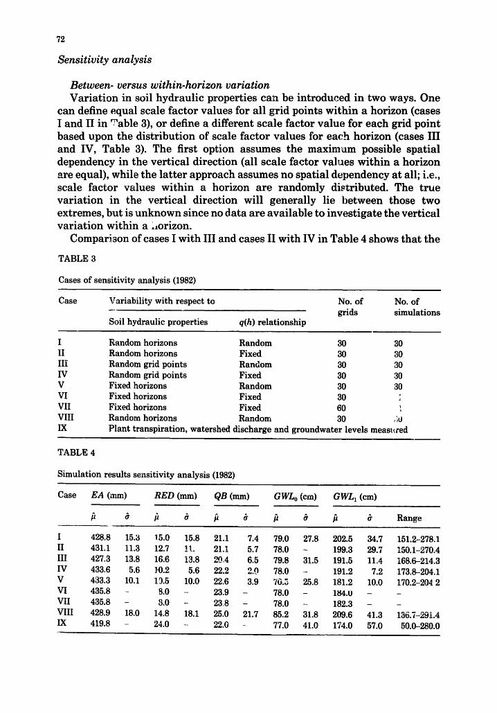
Sensitivity analysis

Between- versus within-horizon variation Variat ion in soil hydraulic properties can be introduced in two ways. One

can define equal scale factor values for all grid points within a horizon (cases I and II in ~able 3), or define a different scale factor value for each grid point based upon the distribution of scale factor values for each horizon (cases III and IV, Table 3). The first option assumes the maximum possible spatial dependency in the vertical direction (all scale factor values within a horizon are equal), while the la t ter approach assumes no spatial dependency at all; i.e., scale factor values within a horizon are randomly distributed. The true variat ion in the vertical direction will generally lie between those two extremes, but is unknown since no data are available to investigate the vertical variat ion within a :,orizon.

Comparison of cases I with III and cases II with IV in Table 4 shows that the

TABLE 3

Cases of sensi t ivi ty analys is (1982)

Case Variabi l i ty wi th respect to No. of No. of

grids s imulat ions Soil hydraul ic propert ies q(h) re la t ionship

I Random horizons Random 30 30 II Random horizons Fixed 30 30 III Random grid points Random 30 30 IV Random grid points Fixed 30 30 V Fixed horizons Random 30 30 V! Fixed horizons Fixed 30 VII Fixed horizons Fixed 60 VIII Random horizons Random 30 .,;tJ IX Plant transpiration, watershed discharge and groundwater levels measl~red

TABLE 4

Simula t ion resul ts sensi t ivi ty ana lys is (1982)

Case EA (ram) RED (mm) QB (mm) GWLo (cm) GWL1 (cm)

/~ b ~ b /~ 6" /~ 6" /~ b R a n g e

I 428.8 15,3 15.0 15.8 21.1 7.4 79.0 27.8 202.5 34.7 151.2-278.1 II 431.1 11,3 12.7 !1. 21.1 5.7 78.0 - 199.3 29.7 150.1-270.4 III 427.3 13,8 16.6 13.8 29,4 6.5 79.8 31.5 191.5 11.4 168.6-214.3 IV 433.6 5,6 J,0.2 5.6 22.2 2.0 78.0 - 191.2 7.2 173.8-204.1 V 433.3 10.1 1[}.5 10.0 22.6 3.9 70.5 25.8 181.2 10.0 170.2-204 2 VI 435.8 - 8.0 - 23.9 - 78.0 - 184.0 - - VII 435.8 - 8.0 - 23.8 - 78.0 - 182.3 - - VIII 428.9 18,0 14.8 18.1 25.0 21.7 85.2 31.8 209.6 41.3 136.7-29i.4 IX 419.8 - 24.0 - 22.0 - 77.0 41.0 174.0 57.0 50.0-280.0

73

variation in water balance components and groundwater levels at the end of the 1982 growing season (GWL1) after 30 Monte Carlo (MC) simulations increases ~i th increasing spatial dependency. Hence, also the range of simulated GWLI increased if all grid points within a horizon had equal soil physical characteristics. Note also that the mean generated groundwater level at the beginning of the growir_g season (GWLo) is approximately equal to the h~,~ value in Table 2. Of all variables in Table 3, only the mean GWL~ is semewhat affected by the choice of variation in soil hydraulic properties. Since the true variat ion within a horizon is unknown, it seems appropriate to consider both extremes in variation of soil hydraulic properties.

Influence of variability in soil hydraulic properties and in q(h) relationship The total variation in water balance components caused by a random

variable q(h) relationship has approximately the same magnitude as the variation caused by random variable soil hydraulic properties (compare cases II and V). However, the variation in GWL, is significantly larger for case II where the soil hydraulic properties only were varied.

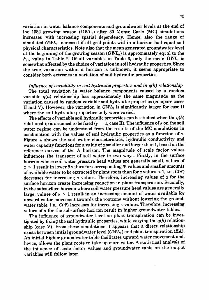
The effects of variable soil hydraulic properties can be studied when the q(h) relationship is assumed to be fixed (7 = 1, case II). The influence of • on the soil water regime can be understood from the results of the MC simulations in combination with the values of soil hydraulic properties as a function of ~. Figure 4 shows the soil water characteristics, hydraulic conductivity and water capacity functions for a value of a smaller and larger than 1, based on the reference curves of the A horizon. The magnitude of scale factor values influences the transport of so:,l water in two ways. Firstly, in the surface horizon where soil water pressure head values are generally small, values of

> I result in lower 0 values for corresponding • values and smaller amounts of available water to be extracted by plant roots than for a values < 1, i.e., C(~) decreases for increasing • values. Therefore, increasing vaJues of • for the surface horizon create increasing reduction in plant transpiration. Secondly, in the subsurface horizon where soil water pressure head values are generally large, values of • > 1 result in an increasing amount of water availsble for upward water movement towards the rootzone without lowering the ground- water table, i~e., C(~) "~ncreases for increasing ~ values. Therefore, increasing values of • for the subsurface hor;zon result in higher groundwater tables.

The influence of groundwater ]!eve! on plant transpiration can be inves- tigated by fixing the soil hydraulic properties, while varying the q(h) relation- ship (case V). From these simulations it appears that a direct relationship exists between initial groundwater level (GWLo) and plant transpiration (EA). An initial higher groundwater table facilitates upward water movement and, honce, allows the plant roots to take up more water. A statistical analysis of the influence of scale factor values and groundwater table o~ the output variables will follow later.

74

10.0t~

---- ~ = 1.25 _/~/~ /

I . . . . 100

~'"~"~ ~ ~. ~. ~ 1 0

\ 'N

I I

I i /

I /

/ , / I

/ /

/

I I

I I

I I

~ i I I I | l I I I | 1 1 I I I I I 0.0075 0.002 0.0015 0.002 0.0005 0 0.05 0.10 0,20

C (cm -I} e{cm3cm -3)

I I I - 10'

/ /

// ! / t ' F

f 10-1

i0"~

F

\

\ / .10-"

I

i , 10 -s 0.30 04

Fig. 4. Soil water characteristic, hydraulic conductivity, and water capacity curves for • values of 0.75 and 1.25, using the reference curves of the A horizon.

Further analysis To verify that a vertical grid spacing of 10 cm results in su~cient ly accurate

results, simulations were performed with a grid spacing of ~0 and 5 cm (cases VI and VII, Table 3). The water balance components of both simulations were close enough to allow a grid point distance of 10cm.

It was furthermore investigated whether the combination of an A-BC profile yielded simulation resul~s different from those when the whole profile would be considered as being characterized by the soil physical properties of the A horizon only (cases I a~d VIII, Table 3). The mean values for cases I and VIII hi Table 4 are almost identical. The variation, however, increases if only one horizon is considered to be representative for the whole profile. The latter

75

result is in a¢:cordance with the larger standard deviation of scale factor values for the A than for the BC horizon (Table 2) and with the result of an increase of spatial dependency.

Finally, all simulation results of the sensitivity analysis (cases I to VIII, Table 4) were compared with the measured water balance com2onents and groundwater levels (case IX). In doing so, it appears that the measured plant transpiration (EA) is smaller than any of its mean simulated values. No such straight comparison is possible for the discharge and groundwater levels, since those were obtained from measurements of the total watershed area, while the simulated results of the sensitivity analysis refer to A-BC profiles only.

Monte Carlo siwu!ations

For each soil profile type, as specified in Table I and illustrated in Fig. 1, 30 MC simulations were performed for the growing season of 1982. Soil profile thickness was assumed to be 3.0m. This thickness was chosen, so that the groundwater table would never exceed this depth. Initial groundwater levels, obtained from eqn. (18), were randomly generated such that they would never be within the first 0.3 m from the soil surface. Shallower groundwater tables could result in ponded water after precipitation, a condition unallowable for the numerical mode]. Also scale factor values for the soil hydraulic properties were truncated such that they were not smaller t h ~ 0.25 and not larger than 2.5. This maximum range of scale thctor values was in accordance with the measured soil hydraulic properties. Values outside this range appeared to cause numerical instability in the simulations.

The statistics for the output variables of this series of M C simulations are listed in Table 5A and B. It shows the mean and standard deviation of the simulated cumulative actual plant transpiration (EA), cumulative reduction (RED) in transpiration from the potential transpiration and the cumulative discharge from the soil profile (QB), as well as the mean and standard deviation in initial and final groundwater levels (GWLo and GWL1) at the beginning and end of the growing season, respectively, for each profile type. Table 5 also lists the measured values of EA (TNO Report, 1984)~ RED and precipitation (measured at meteorological station), and watershed discharge during the simulated growing season. Table 5A shows the simulation results if each grid point within a horizon is assigned a randomly generated scale factor value, while Table 5B shows the same results for randomly generated scale factor values for each horizon.

The output variables of primary interest are EA and RED. Table 5 shows that EA values are not affected by the presence of clay if the clay layer starts at a depth greater than 1.0 m below the soil surface, i.e., the simulation results for profile types 1 and 3 can be combined to yield an average EA value for those soils where the starting depth to clay is larger than 1.0m. Decreasing EA values and thus increasing RED values were calculated for simulations of profiie types 4 and 5. Therefore, the Hupsel watershed can be divided into three

TA

BL

E 5

Res

ult

s M

C s

imu

lati

on

s 19

82 (3

0 si

mu

lati

on

s fo

r ea

ch ~

oil

typ

e) a

nd

197

6 (5

0 si

mu

lati

on

s fo

r ea

ch s

oil

type

)

Soi

l S

tart

ing

dep

th

EA

(m

m)

RE

D (

rnm

) Q

B (

mm

) G

WLo

(cm

) ty

pe

to c

lay

(cm

)

GW

L1 (c

m)

Ran

ge

A.

Spat

ial

vari

able

gri

d po

int,~

(19

82)

1 n

o c

lay

42

7.3

13.8

16

.6

13.8

2'

0.4

6.5

2 14

0 43

0.7

13.7

12

..1

13.7

23

.7

10.5

3

100

430.

1 12

.4

12.8

12

.4

21.0

6.

5 4

60

415.

1 15

.9

28.7

15

.9

22.7

5.

2 5

30

37~.

9 15

.5

67.1

15

.5

23.2

4.

8 M

easu

red

41

~}.8

24

.0

22.0

B.

Spat

ial

vari

able

hor

izon

s (1

982)

1

no c

lay

42

8.8

15.8

15

.~

15.8

21

.1

7.4

2 14

0 42

8.8

16.7

15

.0

16.7

21

.8

17.8

3

100

430.

6 15

.3

13.2

15

.3

17.6

6.

5 4

60

419.

9 16

.9

23.9

16

.9

19.7

8.

2 5

30

381.

4 13

.5

62.4

13

.5

22.5

9.

4 M

easu

red

41

9.8

24.0

22

.0

C. S

pati

al v

aria

ble

hori

zons

(19

76)

79.8

31

.5

191.

5 73

.3

31.2

18

71

~9.4

29

.6

181.

4 G

5.4

22.3

15

2.2

9.0

20.2

14

2.9

(,Pr

ecip

: 25

4.3

ram

)

11.4

15

.5

9.8

9.7

9.9

80.7

26

..7

202.

5 34

.7

74.7

32

.8

198.

6 17

.9

58.3

21

.7

185.

3 19

.5

62.3

25

.9

169.

6 19

.3

64.8

22

.1

1.50

.0

27.0

1 n

o c

lay

42

9.8

36.2

74

.6

36.2

18

.7

9.9

77.6

30

.1

206.

6 2

140

420.

3 42

.4

84.1

42

.4

19.2

9.

6 83

.7

34.4

20

7.2

3 10

0 44

0.6

24.1

63

.8

24.1

14

.0

5.4

60.6

26

.1

194.

7 4

60

391.

9 27

.3

112.

5 27

.3

15.0

6.

0 61

.6

23.4

~7

9.1

5 30

34

6.3

21.0

15

8.1

21.0

15

.9

8.2

58.5

24

.6

163.

6 M

easu

red

36

9.5

134.

9 8.

2 (P

reci

p: 2

13.9

mm

)

Z8.

6 24

.4

19.7

24

.2

28.3

168.

6-21

4.3

161.

7-23

1.3

163.

1-19

8.1

145.

5 -1

80.6

12

3.8-

165.

3

151.

2-27

8.1

166.

9-24

1.1

134.

6-23

0.0

130.

7-21

2.4

103.

6-19

6.2

152.

8-26

6.1

161.

4--2

61.8

15

2.5-

242.

9 ~.

40.I

-263

.6

118.

3-24

3.8

77

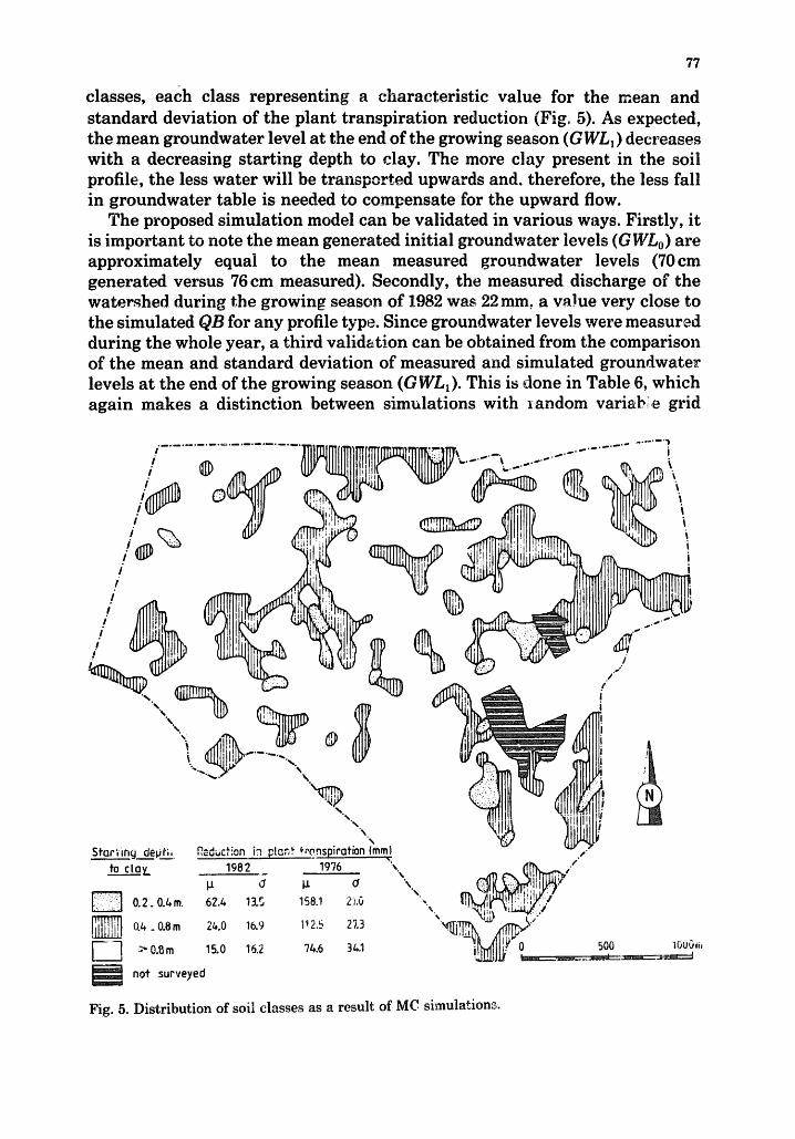
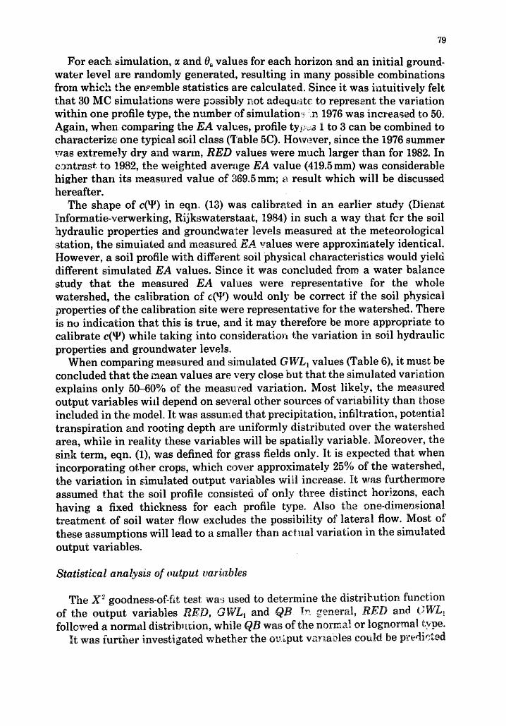
classes, each class representing a characterist ic value for the mean and s tandard deviation of the plant t ranspirat ion reduction (Fig. 5). As expected, the mean groundwater level at the end of the growing season (GWLI) decreases with a decreasing start ing depth to clay. The more clay present in the soil profile,, the less water will be transported upwards and, therefore, the less fall in groundwater table is needed to compensate for the upward flow.

The proposed simulation model can be validated in various ways. Firstly, it is important to note the mean generated initial groundwater levels (GWLo) are approximately equal to the mean measured groundwater levels (70cm generated versus 76cm measured). Secondly, the measured discharge of the watershed during the growing season of 1982 was 22 mm, a value very close to the simulated QB for any profile type. Since groundwater levels were measured during the whole year, a third validation can be obtained from the comparison of the mean and standard deviation of measured and simulated groundwater levels at the end of the growing season (GWL1). This is done in Table 6, which again makes a distinction between simulations with random variab,!e grid

i ....... -:- ............... ~mm,ml~!~2~~T~-....-..-~ ...-.-.-- .............. / ~ ~' , ~ ~ ~ %111~ ~ , ~ ~ ~ ~ ~ ,.,

/ ~ ~ % ~ ~ , - ~ _ itl!lllllllJ41~lrll!illljlrl

• " ll!it A IIIIIV

•

% .% "%

"\ ' \

Sforling d_ept'i._2. P, educflon in ptan, ~rolnspirafion (mini ,,. to cloy_ 1982 1976 "~ \ , : : ~ " ""

0.2. O.l,m 62.a 13.5 158.1 2i.5 ,

FnTnTn I ~ 0.4.0.Sm '~ t ; l #~ 0 500 lOUO,,

i6.9 1!2.5 27.3

16.2 7/~.5 3 a.1 '--] > O.~m 15.0

not surveyed

Fig. 5. Distribution of soil classes as a result of MC simulations.

~48

TABLE 6

Groundwater (cm) levels at end of grov:.ng season: measured versus simulated (weighted by h'action of area representing each profile type, Table 1)

Statistics determined from

MC-simulations

Variable grids Variable horizons

Measured ground- water levels

A. 1982 All profile types combined 179.6 Class-1 tubes only (start- 170.4 ing depth to clay < 1.2 ~n) Class-2 tubes only (strut- !90.4 ing depth to clay > 1.2 m)

16.5 188.0 30.3 174.0 50.0 O 16.2 176.6 ,,0.9 165.0 41.0

12.0 201.5 31.8 193.0 56.0

B. 1976 All profile types combined 195.~ 27.6 191.2 60.0 Class-1 tubes only 185.8 24.0 183.2 58.0 Class-2 tubes only 206.8 27.4. 208.0 61.0

points and hori::ons only. The comparison in Table 6 shows that the mean simulated value~ of GWL, are fairly close to the measured ones. However, as important as tke mean is the simulated variation in GWL, as compared with its measured variation. Since one of the objectives of this study was to quantify the variation in wate~ balance components, the simulated variation in GWL1 should be of comparable magnitude of the measured variation. The results in Table 6 show that appro'Amately 50-60% of the measured variation is explained, if it is assumed t~at the soil hydraulic properties within a horizon de not vary in the vertical direction, while only 25-35% of the measured variation is calculated if each grid point is assigned a random c: value. Therefore, decreasing the spatial structure of scale factor values within a horizon (e.g. by randomly generating ~ values for each grid point) decreases the variation in simulated groundwater levels. The conclusion is in agreement with results from others (Smith and Freeze, 1979b; Andersson and Shapiro, 1983). It is probably more realistic to include within horizon variation only when two dimensional flow is considered. In two dimensions, variation in soil hydraulic properties may cause by-pass flow or create preferential flow paths and, therefore, decrease the ensemble variation in output variables. Finally, simulated E,A yahoos for each profile type were weighted by the fraction of the total watershed area represented by each prGfi]~ type. This weighted average EA vahJe was very ck~e to the EA value measured at the meteoroh~gica! station (425.3 versus 419.8 ram) i~ 1982.

79

For each simulation, ~ and 0~ values for each horizon and an initial ground- water level are randomly generated, resulting in many possible combinations from which the ensemble statistics are calculated. Since it was intuitively felt that 30 MC simulations were p3ssibly not adequate to represent the variation within one profile type, the number of simulationv :,n 1976 was increased to 50. Again, when comparing the EA values, profile tyi:,~s i to 3 can be combined to characterize one typical soil class (Table 5C). However, since the 1976 summer was extremely dry and warm, RED values were much larger than for 1982. In c3ntrast to 1982, the weighted average EA value (419.5 mm) was considerable higher than its measured value of 369.5 mm; a result which will be discussed hereafter.

The shape of c(~P) in eqn. (13) was calibrated in an earlier study (Dienst l[nformatie-verwerking, Rijkswaterstaat, 1984) in such a way that fcr the soil hydraulic properties and groundwa~Ler levels measured at the meteorological station, the simulated and measured EA :,alues were approximately identical. However, a soil profile with different soil physical characteristics would yield different simulated EA values. Since it was concluded from a water balance study that the measured EA values were representative for the whole watershed, the calibration ef c(tP) would only be correct if the soil physical properties of the calibration site were representative for the watershed. There is no indication that this is true, and it may therefore be more appropriate to calibrate c(~) while taking into consideration the variation in soil hydraulic properties and groundwater levels.

When comparing measured and simulated GWL~ values (Table 6), it must be concluded that the mean values are very close but that the simulated variation explains only 50--60% of the measu:ced variation. Most likely, the measured output variables wiJl depend on several other sources of variability than those included in the model. It was assumed that precipitation, infiltration, potential transpiration and rooting depth are uniformly distributed over the watershed area, while in reality these variables will be spatially variable,. Moreover, the sink term, eqn. (1), was defined for grass fields only. It is expected that when incorporating other crops, which cover approximately 25% of the watershed, the variation in simulated output variables will increase. It was furthermore assumed that the soil profile consisted of only three distinct horizons, each having a fixed thickness for each profile type. Also the one-dimensional treatment of soil water flow excludes the possibility of lateral flow. Most of these assumptions will lead to a smalle~ than actual variation in the simulated output variables.

Statistical analysis of output variables

The X -~ goodness-of-fit test wa:~ used to determine the distribution function of the output variabies RED, GWL, and QB T~ general, RED and CWL: followed a normal distribu6on, while QB was of the norma~ or lognormal type.

It was iurther investigated whether the ov~put va)-mbles could be predicted

80

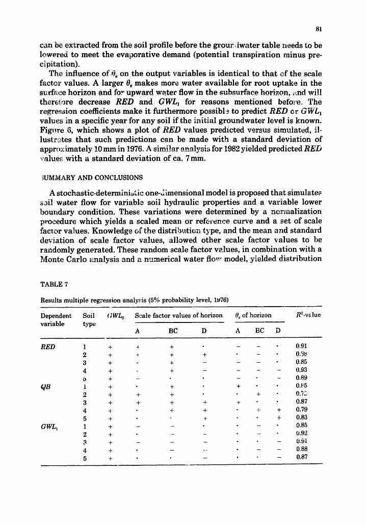
from known input values of initial groundwater level and scale factor and saturated water content values for each horizon. The results of the multiple regression analysis used are shown in Table 7. The signs below each listed independent variable indicates whether a positive (+) or negative ( - ) corre- lation between the ~a~ulated dependent and independer~t variables was signifi- cant. Most ¢;f the significant correlatim~s in Table 7 were already found in the sensitivity analysis.

A deeper initial groundwater level limits upward movement and, hence, increases .~ED and decreases the ;all in groundwater table during the growing sea~ ~ ,n. The ~atter results, therefore, m a larger cumulative discharge QB. Of cm:r~:;e, also GWLo and GWL~ are positively correlated.

Larger scale factor values in the surface horizon will generally lead to smaller amounts of wa~er available for the plants and, th'erefore increase RED and decrease GWL~. However, a larger scale factor value in me subsurface hori~o.n~ ~ight increase upward water flow since the w~saturated hydraulic conductivity concomitantly increases, while GWL~ will decrease as more water

200-

180-

160,

1~0.

1201

~', t

g 1oo

s , :Y

6, /

/ I/~ - /

! --

20 (,0 60 80

o / x X /

x x~Fo T ,.~

'+ +

/ /

o

o

100

, / / o :

).Yo t . /o

÷

,~ A~a/- /

• - ~ 1 u

a / / x x

o

, f

i., , r

/ a

symbol soil type o ! . 2 + 3 x L, a 5

120 %0 150 180 ~ED (ram} simulated

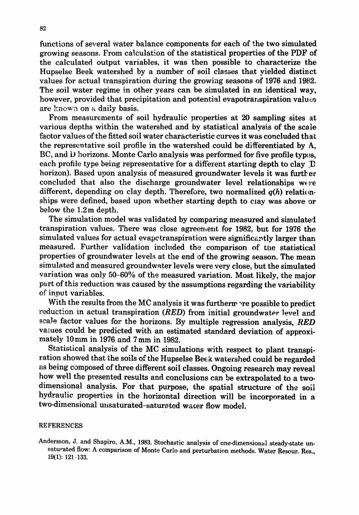
Fig. 6. R J ~ D values simulated verms estimated from multiple regression analysis.

.1__._.____

200

l ine

8 1

can be e x t r a c t e d from the soil profi le before t he g rou r~ iwa t e r t ab l e needs to be lowered to m e e t t he e v a p o r a t i v e d e m a n d (po t en t i a l t r a n s p i r a t i o n m i n u s pre- c ip i ta t ion) .

The i n f luence of 0. on the o u t p u t v a r i a b l e s is i den t i ca l to t h a t ~:f the scale f ac to r va lues . A l a rg e r 08 m a k e s more w a t e r a v a i l a b l e for roo t u p t a k e in the surf~ce h o r i z o n a n d for u p w a r d w a t e r flow in t he subsu r f ace hor izon , ~nd will there iOre d e c r e a s e R E D a n d GWL~ for r e a s o n s m e n t i o n e d before, The r eg re s s ion coefficients m a k e i t f u r t h e r m o r e poss ib ly to p red ic t R E D or Gi,VL~ va lue s in a specif ic y ea r for a n y soil if the i n i t i a l g r o u n d w a t e r level is known . F i g u r e 6, w h i c h shows a p lo t of R E D va lue s p r ed i c t ed ve r sus s imu la t ed , i!o lu s t r~ te s t h a t s u c h p r ed i c t i ons can be m a d e w i t h a s t a n d a r d d e v i a t i o n of app ro ) : ima te ly 1 0 m m in 1976. A s im i l a r ana ly s i s for 1982 y ie lded p red ic t ed R E D va lues w i t h a s t a n d a r d d e v i a t i o n of ca. 7 mm.

iUMMARY AND CONCLUSIONS

A s t o c h a s t i c ° d e t e r m i n i s t i c one -~ imens iona l mode l is p roposed t h a t s imu la t e s soil w a t e r flow for v a r i a b l e soil h y d r a u l i c p r o p e r t i e s and a v a r i a b l e lower b o u n d a r y cond i t i on . These v a r i a t i o n s were d e t e r m i n e d by a n o r m a l i z a t i o n p rocedu re w h i c h yie lds a sca led m e a n or refe~'ence cu rve and a se t of scale fact.or values. Knowledge ~f the distributi(m type, and the mean and standard deviation of scale factor values, allowed other scale factor values to be randomly generated. These random scale factor w.lues, in combination with a Monte Carlo ,malysis and a numerical water flow model, yielded distribution

TABLE 7

Results multiple regression analyris (5% probability level, ls76)

Dependent Soil (iWLo Scale factor values of horizon 0~ of horizon R2-v~ lue variable type

A BC D A BC D

RED 1 + 4 + . . . . 0.91 2 + ~ + + • - • 0 . 3 ~

3 + ~ + . . . . 0.85 4 + - + . . . . . 0.93

+ . . . . . . . 0.89 ~ B 1 + • + • + • • 0 . ~ 5

2 + + + • • + 0.'.,2 3 + + + + + • • 0.87 4 + • + + • + + 0.79 5 + • e • • + 0.83

GWL 1 1 + . . . . . . 0.85 2 + . . . . . . . . U.92 8 + . . . . . . 0.91 4 + . . . . . . . 0.88 5 + . . . . . 0.87

82

functions of several water balance components for each of the two simulated growing seasons. From calculation of the statistical properties of the PDF of the calculated output variables, it was then possible to characterize the Hupselse Beek watershed by a number of soil classes that yielded distinct values for actual transpiration during the growing seasons of 1976 and 1982. The soil water regime in other years can be simulated in an identical way, however, provided that precipitation and potential evapotranspiration valu~:s are knewn on a daily basis.

From measurements of soil hydraulic properties at 20 sampling sites at various depths within the watershed and by statistical analysis of the scale factor values of the fitted soil water characteristic curves it was concluded that the representative soil profile in the watershed could be differentiated by A, BC, and D horizons. Monte Carlo analysis was performed for five profile types, each profile type being representative for a different starting depth to clay :I~ horizon). Based upon analysis of measured groundwater levels it was further concluded that also the discharge groundwater level relationships w(,re different, depending on clay depth. Therefore, two normalized q(h) relati(,n- ships were defined, based upon whether starting depth to clay was above or below the 1.2m depth.

The simulation model was validated by comparing measured and simulated transpiration values. There was close agreement for 1982, but for 1976 the simulated values for actual evapctranspiration were significa,-tly larger than measured. Further validation included the comparison of tim statistical properties of groundwater levels at the end of the growing season. The mean simulated and measured groundwater levels were very close, but the simulated variation was only 50-60% of the measured variation. Most likely, the major part of this reduction was caused by the assumptions regarding the variability of in•vt variables.

With the results from the MC analysis it was furtherw ~re possible to predict reduction in actual transpiration (RED) from initial groundwater ]evel and scaJe factor values for the horizons. By multiple regression analysis, RED values could be predicted with an estimated standard deviation of approxi- mately 10ram in 1976 and 7mm in 1982.

Statistical analysis of the MC simulations with respect to plant transpi- ration showed that the soils of the Hupselse Beek watershed could be regarded as being composed of three different soil classes. Ongoing research may reveal how well the presented results and conclusions can be extrapolated to a two- dimensional analysis. For that purpose, the spatial structure of the soil hydraulic properties in the horizontal direction will be incorporated in a two-dimensional unsaturated-saturoted waker flow model.

REFERENCES

Andersson, J. and Shapiro, A.M., 1983. Stochastic analysis of one-dimensional steady-state un- saturated flow: A comparison of Monte Carlo and perturbation methods. Water Resour. Res., 19(1): 121-133.

83

Arya, L.M., Farrell, D.A. and Blake, G.R., 1975. A field study of soil water depletion patterns in presence of growing soybean roots. I. Det,~rl~'~nation ofhydraalic properties of the soil. Soil Sci. Soc. Am., Proc., 39: 424-430.

Bakr, A.A., Gelhar, L.W., Gutjahr, A.L. and MacMillan, J.R., 1978. Stochastic analysis of spatial variability in subsurface flows. 1. Comparison of one- and three-dimensional flows. Water Resour. Res., 14(2): 263-271.

Belmans, C., Wesseling, J.G. and Feddes, R.A., 1981. Simulation model of the water balance of a cropped soil providing different types of boundary conditions (SWATRE). Nota 1257, ICW, Wageningen.

Bouma, J., ! 977. Soil survey and the study of water movement in unsaturated soil. Soil Surv. In~t~ Wageningen, Soil Surv. Pap., 13: 47-52.

Bresler, E. and Dagan, G., 1983. Unsaturated flow in spatially variable field:~. 2. Applic8tion of water flow models to various fields. Water Resour. Res., 19(2): 421-428.

Clapp, R.B., Hornberger, G.M. and Cosby, B.J., 1983. Estimating spatial variability in soil moisture with a simplified dynamic model. Water Resour. Res., 19(3): 739-745.

Dirksen, C., 1979. Flux-controlled sorptivity measurements to determine soil hydraulic property functions. Soil Sci. Soc. Am., J., 43: 827-834.

Ernst, L.F. and Feddes, R.A., 1979. Invloed van grondwateronttrekking voor beregening en drinkwater op de grondwaterstavd. Nora 1116, ICW, Wageningen.

Freeze, R.A., 1975. A stochastic-conceptuai analysis of one-dimensional groundwater flow in nonunifoi:m homogeneous media. Water Resour. Res., 11(5): 725-741.

Gelhar, L.W., 1986. Stochastic subsurface hydrology from theory to applications. Water Resour. Res., 22(9): 135S-145S.

Gutjahr, A.L. and Gelhar, L.W., ~981. Stochastic models of subsurface flow: Infinite versus finite domains and statiovarity. Water Resour. Res., 17(2): 337-350.

Hopmans, J., i987a. A comparison of various techniques to scale soil hydraulic prop,=ties. J. Hydrol., 93: 241-256.

Hopmans, J., 1987b. Treatment of the groundwater table in the stochastic approach of unsaturated water flow modelling. Agric. Water Manage., 13: 297-306.

Hopmans, J., 1987c. Some major modifications of the simulation model SWATRE. Rep. 79 Dep. Hydraul. Catchment Hydrol.,, Agric. Univ., Wage~.ingen.

Hopmans, J,, and Overmars, B., L986. Presentation and application of an analytical model to describe soil hydraulic prcp,;:::ies. J. Hydroi., 87: 135-143.

HGpmans, J. and Stricker, J.N.M, 1986. Boil hydraulic properties in the study area Hupselse Beck as obtained from three diff~ ~ent scales of observation: An overview. Rep. 78, Dep Hydraul. Catchment Hydrol., Agric. ~ Jniv., Wageningen.

Miller, E.E., and Miller, R.D., ': 956. Physical theory for capillary flow phenomena. J. Appl. Phys., 27(4): 324-332.

Peck, A.J., Luxraoore, R.J. and Stolzy, J.C., 1977. Effects of spatial variability of soil hydraulic properties in water budget modeling. Water Resouro Res., 13(2): 348-354.

Philip, J.R., 1980. Field heterogeneity: Some basic i~,:es~ Water Resour. Res., i0(2): 43~448. Diem:t Informatieverwerking, Rijkswaterstaat, 1984. Herziening van de berekening van de gewas-

verdamping in het hydrologisch model GELGAM. Rep. Ad Hoc Group Transpiratiou, Dienst Informatieverwerking, Rijkswaterstaat, Arnhem.

Russo, D. and Bresler, E., 1980a. Field determinations of soil hydraulic propertie~ for statist:~cal analysis. Soil Sci. Soc. Am., J., 44: 697-702.

Russo, D., and Bresler, E., 1980b. Scaling soil hydraulic properties of a heterogeneous field. Soil Sci. Soc. Am., J., 44: 681-684.

Russo, D. and Bresler, E., 1981a. Effect of fie~d variability in soil hydraulic properties on solutions of unsaturated water and salt flows. Soil Sci. Soc. Am., J., 45(4): 675-681.

Russo, D. and Bresler, E., 1981b. Soil hydraulic properties as stochastic processes: I. An analysis of field spatial variability. ~oil Sci. Soc. Am., J., 45(4): 682-687.

Smith, L. and Freeze, R.Ao, 1979a. Stochastic analy~,s of ~teady state groundwater flow in a bounded domain. 1. One-dimensional s~mulations. Water Resour. Res., 15(3): 521-528.

84

Smith, L., and Freeze, R.A., 1979b. Stochastic analysis of steady state groundwater flow in a bounded domain. 2. Two-dimens~Jnal simulations. Water Resour. Res., 15(6): 1543-1559.

Stakman, W.P., Valk, G.V. ard Van der Harst, G.G., 1969. Determination of soil moisture retention curves. I. Sandbox apparatus. ICW, Wageningen.

Stephens, M.A., 1974. EDF-Statistics for goodness-of-fit and some comparisons. J. Am. Stat. Assoc., 69: 730-737.

Thorn, A.S. and Oliver, H.R., 1977. On Penman's equation for estimating regional evaporation. Q.J.R. Meteorol. Soc., 103: 345-357.

TNO Report, 1984. Comparison of simulation models for unsaturated soil-water transport and plant transpiration. Hydrol. Onderz. TNO, Ser., Rapp. Nota's No. 13 (in Dutch)..

Van Genuchten, R., 1978. Calculating the unsaturated hydraulic conductivity with a new closed- form analytical model. Dep. Cir. Eng., Princeton Univ., N.J., 78-WR-08.

Warrick, A.W. and Amoozegar-Fard, A., 1979. Infiltration and drainage calculations using spatially scaled hydraulic properties. Water Resour. Res., 15(5): 1116-1120.

Warrick, A.W., Mu!len, G.J. and Nielsen, D.R., 1977a. Scaling field-measured soil hydraulic properties using a similar media concept. Water Resour. Res., 13: 355-362.

Warrick, A.W., Mullen, G.J. an:~ Nielsen, D.R., 1977b. Predictions of the soil water flux based upon field-measured soil-,~ater properties. Soil Sci. Soc. Am., J., 41: 414-419.

W~sten, J.H.M., Stoffelsen, G.H., Jeunisser~, J.W.M., Holst, A.F. and Bouma, J., 1983: Proefgebied Hupselse Beek; regionaal bodemkundig en bodemfysisch onderzoek. Rapp. No. 1706, Sticht. Bodemkartering, Wageningen.

W~sten, J.H.M., Bouma, J. and Stoffelsen, G.H., 1985. Use of soil survey data for regional soil water simulauon models. Soil Sci. Soc. Am., J., 49: 1238-1244.

Yeh, T,-C, Gelhar, L.W. and Gutjahr, A.L., 1985a. Stochastic analysis of unsaturated flow ip heterogeneous soils. 1. Statistically isotopic media. Water Resour. Res., 21(4): 447-456.

Yeh, T.-C., Gelhar, L.W. and Gutjahr, A.L., 1985b. Stochastic analysis of unsaturated flow in heterogeneous soils. 3. Observations and applications. Water Resour. Res., 21(4): 465-431.