- 1 -

StellarNet

Miniature Spectrometer Manual

Universal Spectroscopy Solutions For Laboratory or Field Measurements

14390 Carlson Circle, Tampa, FL 34677

Phone 813-855-8687 Fax 813-855-2279 www.StellarNet-Inc.com

- 2 -

CC Declaration of Conformity According to EN45014

We

StellarNet, Inc.

of

14390 Carlson Circle Tampa, Florida

USA

Declare under our sole responsibility that the products named below conform to the following standard(s) or other normative document(s):

Product name: Miniature Fiber Optic Spectrometer

Product type: Spectrum Analyzer

Product models: BLUE-Wave, BLACK-Comet, RED-Wave, DWARF-Star, GREEN-Wave, EPP2000 HR, EPP2000 UVN-SR, Dual DSR

Safety: EN61010-1, EN61010-2-031, IEC61010-3-1

EMC: EN61326 + A1

Supplementary information: The product complies with the requirements of the Low Voltage Directive 73/23/EEC-93/68/EEC, and the EMC Directive 89/336/EEC-92/31/EEC and 93/68/EEC.

Will Pierce President StellarNet, Inc. January 2, 2011

- 3 -

Table of Contents

5 Introduction

8 Quick Start Installation for SpectraWiz Software and USB cable drivers for

Windows

10 SpectraWiz Software General

10 Help

10 Software Capabilities

10 Experiment Procedures

13 Toolbar Icons

15 Application Icons

16 Status Bar

17 SpectraWiz File Menu

17 Save

18 Open

18 Print

19 SpectraWiz Setup Menu

19 Detector integration time

19 Number of scans to average

20 Spectral smoothing controls

21 Temperature compensation

21 X Timing resolution control

21 Episodic Data capture

22 Optical Trigger

22 Spectrometer channel

23 Actions for peak icon

23 Display Refresh rate

23 Channel display trace

23 Graph Print Info Prompts

23 Interface Port and detector

24 Unit calibration coefficients

24 Warning message enable

25 SpectraWiz View Menu

25 Scope mode

26 Absorbance mode

26 Transmission mode

26 Irradiance mode

27 Ref spectra

27 Channel

27 Multi-Graphs

27 Snap Shot

27 Wave Ratio

28 Y scale

28 Zoom

29 Graph Trace as

- 4 -

30 SpectraWiz Applications Menu

30 CIE Color Monitor

32 ChemWiz Methods

32 Solar + Ultra Violet Monitor

33 Irradiance Calibration

35 Quick Guide for Transmission/Absorbance Measurements

35 Using a Cuvette

36 Using a Dip Probe

37 Using a Transmission Fixture

38 Quick Guide for Reflectance Measurements

38 Using a Reflectance Probe

39 Using a Reflectance Fixture

40 Tutorial

40 Configuring SpectraWiz Dual System

41 Importing Data into Microsoft Excel

43 Irradiance calibration using SpectraWiz

51 Trouble-Shooting and Frequently asked Questions

- 5 -

Introduction

StellarNet builds ruggedized miniature fiber optic spectrometers for a complete spectrum

of Lab and Field measurements. Coupled with our fiber optic sampling accessories and

free SpectraWiz® software, you will have accurate and reliable instrumentation for a

multitude of light measurement applications in the UV-VIS-NIR wavelength ranges

anywhere from 190-2300nm. Our company focus is to provide our customers with high

performance instruments excelling in durability, portability, size, and low price.

When used for spectroscopy applications, the instrument can provide wavelength

information used to compute sample absorbance, transmittance, reflectance and emittance

(such as fluorescence, plasma, laser induced breakdown, and Raman spectroscopy). In

addition, these spectrometers are used to measure spectral emissions from various light

sources such as LED’s (Light Emitting Diodes), laser diodes, plasma furnaces, arc lamps,

high and low pressure gases, and solar irradiation. Common Configured systems are

listed below:

• SpectroChemistry Systems

• SpectroRadiometer Systems

• Color Measurement Systems

• Low Cost Fluorescence Systems

• LED Measurement Systems

• PORTA-LIBS Element Analyzer

• Thin Film Measurement Systems

• NIR (Near Infra-Red) Analyzers

• OEM spectrometers UV-VIS & NIR

The spectrometers can provide 2048, 1024, and 512 wavelengths, depending on detector

array selected, for each scan over the factory configured wavelength range. The range

and coarse resolution are determined by the installed diffraction grating groove density,

often referred to as the number of lines per millimeter. The fine resolution is determined

by the installed slit size. The portable spectrometers connect to a computer’s high speed

USB port.

For multi-beam applications, up to eight units may be connected via USB-2

simultaneously. All spectrometers enable optical signal input via single strand optical

fibers with standard SMA 905 connector.

A variety of spectrometer models can be found on the StellarNet website

www.StellarNet.us. Please check the website for detailed specifications. Additionally

StellarNet offers a complete line of fiber optic accessories such as light sources, fiber

optic cables, and sampling accessories for chemistry, radiometry, colorimetry, and optical

measurements.

- 6 -

Popular spectrometer models include:

BLACK-Comet Series- “Holographic, Concave Grating” 2048 pixel CCD with ranges

(C) 190-850nm (CXR) 280-900nm, (C-SR) 200-1080nm, and (CXR-SR) 220-1100nm

BLUE-Wave Series (15 models)-“Holographic and Ruled” 2048 pixel CCD with ranges

200-1150nm.

DWARF-Star and RED-Wave NIR InGaAs Series (cooled 512 and 1024 PDA) with

range 900-1700nm and 900-2300nm, respectively.

EPP2000-UVN-SR “Extreme Grating” 2048 element CCD High Resolution model with

range 200-1100nm

BLACK-Comet Concave Grating Spectrometer- “Research Grade” Optics

The concave grating provides superior optical imaging and has many benefits over other

standard optical techniques (Czerny turner) designs. Among the advantages are decreased

stray light, uniform resolution, improved spectral shapes, and increased sensitivity. A flat

field is projected onto the detector array directly, thus avoiding the focus of scattered

light into the focal plane. An additional intrinsic aberration correction deems it worthy of

being called “Research Grade” for spectrometer optics in a small ruggedized package.

In order to precisely control optical resolution, a slit is permanently installed in the fiber

optic connector. This allows the instrument to maintain resolution when a different fiber

size is connected. Optical resolution determines the instrument’s ability to resolve

adjacent spectral peaks which (for example) could relate to component concentrations or

identify elemental composition in plasma analysis.

Resolving-power Resolution (RR):

When closely spaced spectral peaks are clearly resolved via RR (such as the 577nm +

579nm Mercury doublet) they can be seen to be separated at Half the Max peak height

(HM). The distance between the peak and where its slope intersects the HM position is

defined as the resolving resolution in nanometers.

In a spectrograph with a perfectly imaged detector array, the RR will be the nm/pixel

dispersion. Larger slits decrease resolution as the image spreads to adjacent detector

pixel elements.

Line-width Resolution (LR):

When a single peak is measured at its Full Width Half Max (FWHM), the difference

where the slopes intersect the HM is the Line-width resolution in nanometers.

Conversion from LR to RR use: LR ~= 2 x RR.

- 7 -

StellarNet estimates the spectrometer optical resolution using RR (Resolving-power

Resolution) for standard spectrometer models and FWHM for the HR (High Resolution)

series spectrometers.

The detector arrays include 2048 pixel CCDs (Charge Coupled Devices), or 512 /1024

pixel NIR-InGaAs PDAs. Detector specifications for various spectrometer models are

available on the StellarNet web site. Sensitivity for these devices is extremely high and

range from 100 to 200 V/ (lx * s) as found in the detector manufacturer’s specs (eg:

Sony/Toshiba/Sensors Unlimited). The most common detector array has 2048 elements

with 14um x 200um tall pixels each with a 14um pitch. The NIR InGaAs detector pixels

are 25um x 500um tall pixels with a 25um pitch.

The SpectraWiz software enables detector integration time selections down to 1-3ms

depending on electronics.

- 8 -

Quick Installation for SpectraWiz Software Summary

1. Installation of USB cable drivers for Windows >Note: 64bit Windows not yet available

a) Attach USB cable to spectrometer. b) If available, attach UP5V power to spectrometer.

c) Attach USB cable to available USB port on PC (or USB hub).

Insert StellarNet CDROM and allow WinXP to search for a suitable driver on CDROM.

If not WinXP, specify driver location on CDROM = \SWDrivers10 then select folder:

\SWDrivers-USB2-Spectrometers or \SWDrivers-USB1-GREEN-Wave

Then finally select the driver for your Windows version:

For Win2000, XP, Vista, 7 select folder named “WinXP-Vista-7”

For Win98, Me select folder named “Win9x”

Use Device Manager to verify “StellarNet Spectrometer” is listed under USBDEV device.

Right click on MyComputer then select Manage, then select Device Manager.

Windows 7 users may see “unknown device” listed and will need to click “Update driver”

and specify driver location as specified above.

If Device Manager says “spectrometer - start” you’ll need to select “Update driver”.

If you have the time, it is smart to repeat the cable installation for each USB port on your

PC. Windows 7 users don’t need to do this.

2. Install SpectraWiz using SWUpdate.exe from website (for most recent version).

If web not available then install SpectraWiz using SWUpdate-Install.exe from CDROM

Click on SpectraWiz desktop icon to start, then verify continuous spectral graph display

updates appear with spectrometer attached, then exit SpectraWiz.

Win2000 only: after installation completes, goto SpectraWiz folder, click on Fix2000.bat.

For operation as a SpectroRadiometer goto step 3. If you received an HR spectrometer or

label on the CD marked “SNS –nnnnn.exe”, click on this file. Otherwise, install the

wavelength coefficients listed on spectrometer label using “Setup -> Unit Calibration”

menu. See reverse side for detailed instructions.

Please note if you have BW-16 listed on spectro label the coefficients will load automatically.

3. Install intensity calibration files for SpectroRadiometer operation

The Radiometer calibration files are installed by clicking on the file “MyCal-nnnnn.exe”,

(found on the CD) where “nnnnn” = spectrometer serial # shown on label.

Start SpectraWiz and verify continuous spectral graph display updates appear.

Get going FAST -->>> WATCH the SpectraWiz software training videos on CDROM !

Driver and software updates are easily downloaded from the StellarNet website

a. All drivers are in SWDrivers password=”wdrivers”

b. SWUpdate for all Windows vers password= no password get the latest version now

Additional information is available in the Spectrometer Manual on the StellarNet CDROM.

For PARALLEL cable installation see “Parallel cable installation.doc” on CDROM.

For StellarNet technical support, Phone: 813-855-8687 or email: Support@StellarNet.us

- 9 -

>>Use info found on bottom unit label

1. Open SpectraWiz and select the “Setup” menu then select “Unit Calibration

Coefficients.”

2. Enter 1 at the channel prompt and then enter C1, C2, C3, and C4 values which are

listed on the bottom label of the spectrometer. If no C4 is listed on the label then

enter 0.

3. Select: “Setup” “Interface and Port Detector.”

a) Always check USB2EPP cable unless using the GREEN-Wave spectrometer. If

using a GREEN- or BLUE-Wave, select the appropriate choice.

b) Select the digitizer type listed on bottom of the spectrometer. These are

LT12/LT14/LT16. If the digitizer is not listed, do not select any.

c) Select detector type; default is CCD 2048 unless otherwise stated on label.

4. Now, exit SpectraWiz for the changes to take effect. Start SpectraWiz and verify

continuous spectral graph display updates appear.

For further instruction -->>> WATCH the SpectraWiz Application videos on CD !!

Software Configuration

- 10 -

SpectraWiz Software General Help

Software Capabilities:

SpectroRadiometric Calibrations:

Perform irradiance calibrations for UV-VIS-NIR

Use SL1-CAL lamp or your NIST traceable lamp

SpectroRadiometer measurements:

Irradiant watts per square meter per nm

Irradiant microwatts per sq centimeter per nm

Illuminant LUX - lumens per sq meter per nm

Illuminant foot-candles - lumens per sq foot /nm

Moles per square meter per nm per second as

PAR photosynthetic active radiation 400-700nm

Power Spectral Density with selectable regions

Radiant & Luminous FLUX with selectable area

LED xy chromaticity, dominant λ, purity, mcd

Color rendering graph with rapid sample logging

Correlated color temperature & CRI index

SpectroChemistry measurements:

Analyte concentrations via cuvette & dip probes

PLS calibration method save & recall

Concentration display with rapid sample logging

UV Monitor measurements:

UVa, UVb, UVc, UV a/b ratio, Total Irradiance

Power UVb, Power VIR, Te Erythema minutes

U.S.FDA & European tanning algorithms

Real-time display with rapid sample logging

SpectroColorimeter measurements:

CIELAB L* a* b* for reflectance/transmittance

1931 xy chromaticity diagrams for radiometry

Delta E* comparator signals color differences

SpectroColorimeter (cont’d):

Save and load color standards for Delta E* signal

Color rendering graph with rapid sample logging

Supports master and standard white referencing

XYZ tri-stimulus, xy chromaticity, chroma, hue

Spectroscopy measurements & support:

Transmission %T, Absorbance AU, Reflectance

Episodic data capture & Time series analysis

Dual and multi-beam lamp drift correction

Single-beam relative and absolute drift correction

Spectral ratio display with selectable wavelengths

First and second spectral derivatives

Export spectra to Excel, Matlab, and Galactic

Open, graph, zoom, and print up to 8 spectra

Up to 8 spectrometers display on a single graph

Optical spectrum analysis tools:

Display FWHM, centroid, and peak wavelengths

Power spectral density via manual cursor setup

Zoom x-axis, zoom xy window, y-auto scale

View y-axis as log or linear scale

Optical trigger event setup for spectral capture

Episodic capture can save via optical trigger event

Experiment Procedures:

-First, connect the spectrometer and the accessories to be

used. (Refer to setup diagrams found later in this manual for

details on configuration)

-Plug the +12V power cable into the back of the light source

(if used).

- Plug the +5V power cable into the back of the spectrometer

(Note: only for spectrometers with +5V power cable input).

- Plug USB cable into the back of the spectrometer unit.

-Plug the other end of the USB cable into the computer.

Next, it is necessary to enter the correct interface and port settings.

-Go to Setup Interface and port detector.

- 11 -

Always have a check for USB2EPP cable.

Check the box next to the digitizer and detector type the spectrometer unit contains.

New model spectrometers automatically load calibration coefficients. However, double

check this by starting the SpectraWiz program and entering the 3 calibration coefficients.

Go to Setup Unit calibration coefficents and enter a value of 1 at the channel prompt

(and subsequently 2, 3…8 if you have multiple units connected).

Enter the C1, C2, C3, and C4 (if listed) values on the next prompts. These values are

found on the bottom of each spectrometer. This information tells the software how to

provide the wavelength readouts. If no C4 value is found on spectrometer label, enter 0

for C4.

If you are interested in emission applications (i.e.: looking at light sources, LED’s, laser

diodes, plasma, or fluorescence), you can start measuring right away in "Scope mode"

which is the default view mode at start-up. For applications requiring spectroscopy

modes such as Absorbance, Transmission, or Reflectance (same as Transmission), select

the proper "View mode" after taking a Dark (Black bulb) and Reference (Yellow Bulb)

scan.

Note: the "Black bulb" and the "Yellow bulb" icons are located on the toolbar.

Taking a Dark scan for the Scope mode becomes important with detector integration

times well above 250 ms (above ¼ second). Although it is not required, doing so will

eliminate detector structure baseline, which is a pixel non-uniformity constant. Always

take a "new dark" after changing system parameters such as samples to averaging,

smoothing, and/or detector integration. To take a dark scan, you must block the light

signal input to the spectrometer or turn off the light source. You can then left click with

your mouse on the “Dark bulb” icon. Also, ensure that the Temperature compensation

selection in the setup menu is turned on (enabled). This feature evaluates the dark level

in the "optical black" region of the detector and removes this level from the input signal

on an ongoing basis. This eliminates the need for a dark level shutter.

There is another approach for releasing the Dark scan. This is done if you want to retake

a dark reference. Instead of using the left mouse click on the Dark light bulb icon, use a

right click to "release the Dark." You will see the baseline rise. Now, you can retake

your dark reference.

In all modes, X-zooming and Y-rescaling allow regions of interest to be easily viewed.

Remember, X-zooming allows exclusion of areas that may cause auto Y-rescaling to fail

because of large peaks on left or right. A little "hands on" allows simple navigation with

the tool bar.

Before "viewing" Absorbance or Transmittance you must first setup some basic system

parameters and save a "dark" and "reference" scan. This is performed in the default

"Scope" view mode.

1. Setup and turn on your reference light source so that you are now viewing a

bell shape curve in Scope mode (see picture below). For reflectance, using a fiber

- 12 -

probe, hold the probe at 45o to your white standard, at a distance of about ¼”. For

cuvette holders, use cuvette in place with reference sample solvent. For dip

probes also use your solvent solution for reference.

The curve MUST NOT touch the top of the graph.

If the slider bar on the toolbar is already max (for fastest detector integration rate),

then you must reduce the input signal by using a smaller fiber or inserting a filter.

For reflectance, move the tip back from the white standard (reference) surface.

For others, you may test this out by backing away the SMA 905 fiber optic

connector from either the light source or spectrometer.

2. We recommend you start with (and setup) the following configuration until you

are familiar with the options.

Use the Setup menu:

Detector integration rate = 50 ms

Number of Scans to average = 5 (if below 100 ms integration time)

Pixel resolution (smoothing) = 0 (NONE)

Temperature Compensation = 1 (ON)

Note: if the first 3 items are changed, then you MUST AGAIN save a new "dark"

and "reference" scan.

Increase

integration time

Increase integration

time

Increase

integration time

“Over-saturated” “Optimum Integration Time”

- 13 -

3. Adjust the detector integration until the bell curve fills 95% of the graph. The

longer the detector integrates, the larger the input signal is. The goal of setting

the integration time is to obtain the highest signal without any wavelength going

off scale. Perform a File Save Reference from the menus or click the

yellow light bulb icon on the toolbar.

4. Now block the light at your light source. If you cannot do so, then you will

have to turn off your light source for a moment. Perform a File Save Dark or

click the dark light bulb on the toolbar. Now turn the light source back on and

click the “light bulb” icon to set your reference.

5. At this point you are ready to view Absorbance or Transmission using the View

menu selection. Absorbance and Transmission should appear as flat lines. Insert

your sample and observe the response in real-time. You may now save to disk or

print the sample graph.

Toolbar Icons:

File open

Click to open saved file, this is the same as menu, File->Open->Sample

Save sample spectrum

Click to save the spectra, this is the same as menu File Save Sample (to

disk

Print graph

Left click to print graph.

Snapshot spectra

Left click here to freeze graph trace; Left click again to resume; Right click to

copy graph to Windows clipboard

Save dark spectrum (used for Absorbance, Transmittance, and Irradiance modes).

Left Click after turning off light source;

Right Click to release previous dark (zero)

Save reference spectrum (used for Absorbance and Transmittance modes).

Left Click after turning light on without sample in place or with white

reference.

When viewing Irradiance watts per square meter, clicking here starts the

UV monitor application.

- 14 -

Move Data Cursor Left

Move Data Cursor Right

After placing the data cursor (by pointing and clicking the right button), each

subsequent click, using the left button, will move 1 pixel in direction selected.

To remove data cursor click to left of graph. Clicking the right button on

these icons will seek to the next peak in the selected direction, and place the

data cursor there.

Zoom wavelength

A reminder on how to X- and Y-zoom.

Left click here again to un-zoom.

Left click on the left side of graph to un-zoom.

Right click to enable Y-zoom mode.

Re-scale Y axis

Left click to auto scale Y-axis.

Right Click to undo auto scale Y-axis.

Also use View Y set scale menu to override auto scale with selected scale.

Compute Area

Left click to show the AreaPSD, Centroid, Peakwave, FWHM, and Centbase

of a peak. If the data cursor is not on a peak, the icon will seek to a peak in the

closest direction.

Right Click to start dual data cursor measurement as outlined below.

This information is printed in the graph title (concatenated to end of line)

when printing a graph.

Compute Area toolbar function details

1. Use left mouse click to compute and display: AreaPSD, Centroid, Peakwave,

FWHM, and Centbase (automatically selects closest peak & finds baseline).

o AreaPSD = integral Area (Power Spectral Density).

o Centroid = center wavelength of AreaPSD in nm.

o Peakwave = wavelength of the tallest point.

o FWHM = Full Width Half Max of peak in nm.

o Centbase = level used to compute AreaPSD & Centroid.

2. Use right click to start dual cursor measurement for: AreaPSD, Width, Base

(via the user positioned cursors)

a. Position data cursor to right of area to measure, using right click on

the graph at desired location.

b. Then right click Area toolbar icon and this will

change the data cursor to a dashed line.

- 15 -

c. Now position a second data cursor to left of area

at desired location on graph with right click.

d. Right click Area toolbar icon to display the

AreaPSD, Width, and Base measurements.

e. Right click Area toolbar icon to resume with

normal data cursor as a solid line.

Auto-Integration

Left Click to automatically adjust detector integration time and averaging

using reference light source in scope mode

Detector Integration Time

Left click to set detector integration time

Integration Time Bar

Slide bar with mouse to manually configure the integration time.

Moving the bar to the left, decreases the integration time.

Moving the bar to the right, increases the integration time.

Application Icons:

Solar Monitor

Starts Solar/UV light monitor Application

CIE Color Measurement

Starts CIE color measurement Application

ChemWiz Chemistry

Starts ChemWiz Chemistry Application

Click on these words to quickly switch modes; this is equivalent to selecting the View

menu options:

Scope = View -> Scope mode

AU = View -> Absorbance

%T:R = View -> Transmission (or reflectance)

Watts = View -> Radiometer -> watts

Lux = View -> Radiometer -> Lumen

- 16 -

Solar/UV = Application -> Light Monitor (Solar/UV)

Color = Application -> CIE Color Measurement

Chem = Application -> ChemWiz Methods

Status Bar:

Observe the system indicators appearing below the graph in the status panel.

SCOPE Currently selected mode (also TRANS/ABSOR/REFS/IRRAD)

Wave: Wavelength at the data cursor location

Pix: Location of the data cursor (0-2050 pixels)

Val: Magnitude/value at the data cursor

Time: Detector integration period in milliseconds (ms)

Avg: Number of samples averaged

Sm: Pixel smoothing 0 = none

1 = 5 pixels

2 = 9 pixels

3 = 17 pixels

4 = 33 pixels

Z: An x-axis zoom has been performed

Y: A Y-rescale or Y-zoom has been performed

Y: Y-zoom mode has been enabled

Tc: Temperature compensation on/off

Xt: XTiming resolution control selected

Ch: Shows which channel is selected

- 17 -

SpectraWiz File Menu:

Save: Save current spectra sample data to disk file

Open: Open spectra file for graph display & print

Print Setup: Allows page layout selections for graph

Print: Print current graph sample data to print device

Exit: Terminate SpectraWiz program

File Save:

Allows the user to save spectral data to files. The options are Sample, Reference, Dark,

and Export. Access via File Save menu, disk icon , or Alt + Disk menu

File Save Sample:

In Scope mode: Sample saves “filename.SSM” files

Trans mode: Sample saves “filename.TRM” files

Absor mode: Sample saves “filename.ABS” files

Irrad mode: Sample saves “filename.IRR” files

The Sample files are text and can be read into a spreadsheet program such as Excel using

the "delimited" option using the "space" delimiter. The output format is wavelength (x-

axis) <spaces> value (y-axis) <new line>

The File Save Sample dialog allows the user to select the filename to create. This

dialog has a "Save as type" pull down selection. Using this feature you can save the file

as a Galactic Industries - Grams/32 SPC file. These files can be dragged from the

Windows Explorer "SpectraWiz" directory onto the Grams/32 graph program with the

click of your mouse.

File Save Reference:

File Save Dark:

The Reference file "SW.REF" and Dark file "SW.DRK" are saved when setting up an

experiment that requires the Absorbance or Transmission modes.

- 18 -

The save icons on the toolbar perform same functions for above features very quickly.

Refer to General Help for more detail on this.

The File Save Export selection allow the user to setup the "starting", "increment",

and "ending" wavelengths. This feature linearizes the output data. This allows output

wavelengths to be evenly spaced, and can be enabled or disabled. When disabled, the

wavelength for each detector pixel is output. The wavelengths will not be evenly spaced

due to the dispersion of the spectrograph.

Using Alt+D to save to disk (or clicking on the horizontal menu item "Disk") you can use

the auto filename increment feature. Each time you specify a basic filename, subsequent

saves will append a number to the name, saving you time.

When multiple channels are enabled, a file save sample automatically saves all

channels. This occurs ONLY when the VIEW Multi-Graphs has first been enabled.

Each channel will then append its channel number. For example if the file name to save

is given as TEST and you are in absorbance view, then the files for a 3 channels

configuration will be saved as Test-c1.abs, Test-c2.abs, and Test-c3.abs.

File Open:

Allows the user to select various files to be read back in which were previously stored

using the Save function. The graph may be zoomed or printed. The system is placed in

the "SNAP" mode. To return to normal operation click on the camera icon (which turns

SNAP off).

The Open Command allows multiple spectral traces to be graphed at the same time. To

select multiple files to graph, press and hold the Ctrl key while highlighting the file

names to be graphed. This is a standard way of selecting multiple files in Windows. Each

spectral trace is graphed in a different color. Trace colors can be configured via Setup

Channel Display.

Select the .ep file type to view an episodic data capture. This will display a series of

spectral traces in 3d from the file that was created using the Setup => Episodic data

capture feature. Alternately, you may select specific wavelengths to be extracted and

graphed as time series. The time series data can then be saved to file as .ts file types - one

at a time. Each file will represent action for a selected wavelength over the episodes

time. The .ts files can be opened and graphed in multiple. It is suggested that these files

are named appropriately when saved. The .ts file types can be imported into Excel

because they are in text using space delimited format for timestamp and value.

File Print:

Allows the user to plot the currently selected screen on the connected printer device. A

graph title is optional and will print with date.

Graph print information can be optionally configured using the Setup menu. Up to 4

items can be requested from the operator each time the print option is selected. This

information will be printed as the graph title line. It is primarily used for QC of samples,

where the information includes serial or batch number, temperature, etc.

- 19 -

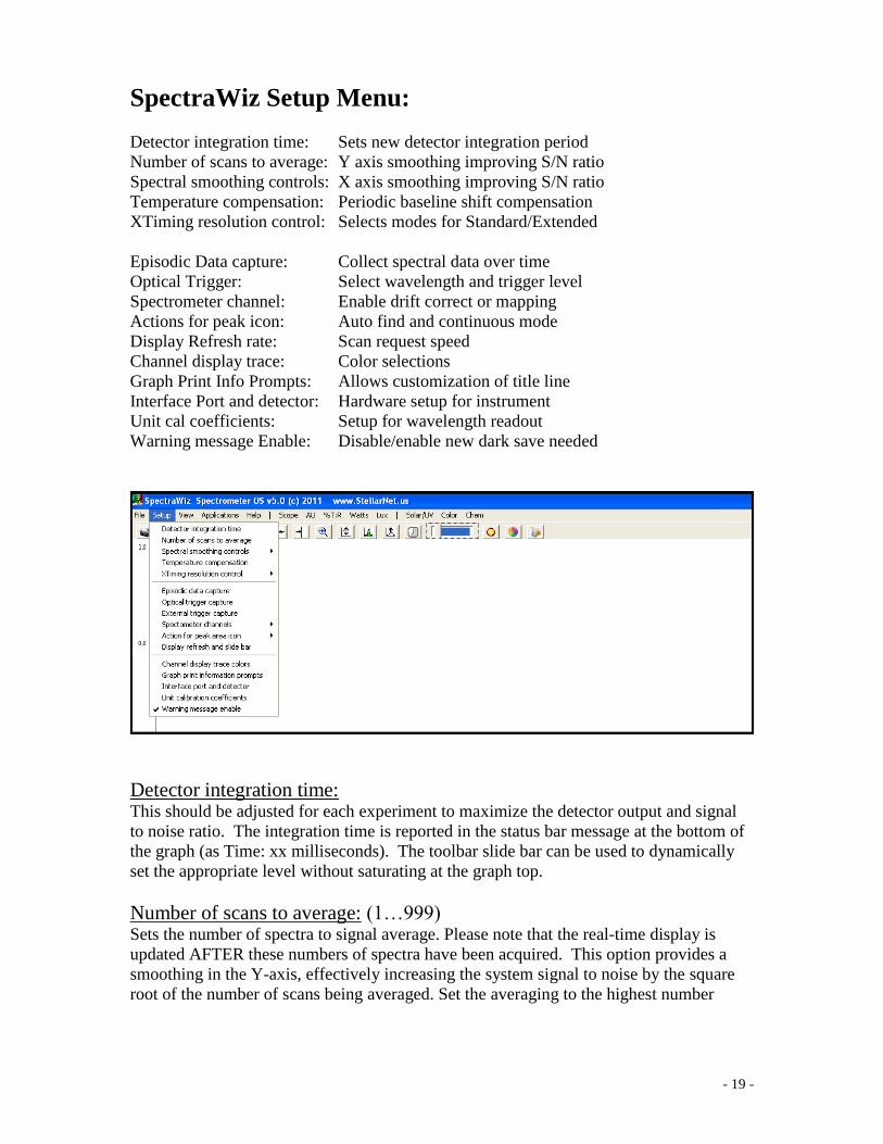
SpectraWiz Setup Menu:

Detector integration time: Sets new detector integration period

Number of scans to average: Y axis smoothing improving S/N ratio

Spectral smoothing controls: X axis smoothing improving S/N ratio

Temperature compensation: Periodic baseline shift compensation

XTiming resolution control: Selects modes for Standard/Extended

Episodic Data capture: Collect spectral data over time

Optical Trigger: Select wavelength and trigger level

Spectrometer channel: Enable drift correct or mapping

Actions for peak icon: Auto find and continuous mode

Display Refresh rate: Scan request speed

Channel display trace: Color selections

Graph Print Info Prompts: Allows customization of title line

Interface Port and detector: Hardware setup for instrument

Unit cal coefficients: Setup for wavelength readout

Warning message Enable: Disable/enable new dark save needed

Detector integration time: This should be adjusted for each experiment to maximize the detector output and signal

to noise ratio. The integration time is reported in the status bar message at the bottom of

the graph (as Time: xx milliseconds). The toolbar slide bar can be used to dynamically

set the appropriate level without saturating at the graph top.

Number of scans to average: (1…999) Sets the number of spectra to signal average. Please note that the real-time display is

updated AFTER these numbers of spectra have been acquired. This option provides a

smoothing in the Y-axis, effectively increasing the system signal to noise by the square

root of the number of scans being averaged. Set the averaging to the highest number

- 20 -

Recommendations: Integration Time Sample Average

1-100 ms 10

100-500 ms 5

500+ ms 3

Spectral smoothing controls: Pixel Boxcar smoothing level 0, 1, 2, 3, or 4

This performs data smoothing by applying a moving average of adjacent pixels to

the data arrays. For example, a Pixel Boxcar setting of 1 would average 5 total

pixels: 2 pixels on the left, 2 pixels on the right, and one in the center. 0 performs

NO data smoothing.

Boxcar setting Total pixels averaged

0 0

1 5

2 9

3 17

4 33

Savitzky Golay level 0, 1, 2, 3, or 4

A spectral smoothing algorithm which performs a local polynomial regression on

a distribution to determine the smoothed value for each point algorithm that

avoids crushing peaks (Savitzky A, Golay M J E. Smoothing and Differentiation

of Data by Simplified Least Squares Procedures. Analytical Chemistry, 36: 1627-

1639, 1964).

S-G setting Total pixels smoothed

0 0

1 9

2 13

3 17

4 21

Display Persistence level: 0…9

This controls smoothing for digital readout displays using exponentially smoothed

averaging. For example, spectral data is used to compute the ChemWiz

concentration for selected methods.

Average dark baseline: checked=ON

This controls the baseline average level to keep it above zero. The algorithm

computes the average dark level and makes the average the zero baseline. Using

long detector integration times will move this level higher using "Scope mode".

When measuring fluorescence it may be desirable to set this feature off so the

baseline is maintained at a real zero level.

- 21 -

Temperature compensation: checked=ON The first 15 "optical black" pixels that are read from the detector provide a useful level of

the sensor dark current even when the detector is illuminated. If this option is on, the

system periodically samples this area and makes an adjustment to the normal readout.

When the level raises or lowers with temperature, the scan is adjusted accordingly.

XTiming resolution control: 1/2/3 This feature provides increased optical resolutions. Selection 1 is the lowest optical

resolution and is synchronized with the selected detector integration. In general, if your

requirements for optical resolution are greater than 1nm, then selection 1 is ok.

Selection 2 or 3 slows the digitizer & detector clock by a factor of 2 and 4 respectively.

With XT levels 2 & 3 you will be able to observe increasingly higher resolutions. The

detectors signal amplifier improves with slower throughput. When selecting XT level 2/3

the detector integration time must be increased to 30ms or longer to avoid sync delays.

Episodic Data capture: This function saves spectral data over a defined time period. It allows a specific number

of episodes to be saved or can be continuous. For continuous scans,the operator can

signal when to stop by clicking on the dark light bulb button.

A time delay can be inserted between each capture and the data can be graphed in 3D

using the File Open function and selecting the .ep file type. When the user specifies

the file name such as "test", then a file test.ep1 will be created. If there are additional

channels active (up to 8), additional files will be created such as test.ep2 (up to test.ep8).

Each file contains an internal time stamp with millisecond resolution.

The .ep files are not in text format;

however the data can be extracted into

text form as a time series. Use File

Open to perform the extraction of a

selected wavelength over time, then save

it as a time series (.ts) file type.

Episodic data files can be converted into

text files, by downloading and installing

the free software package called

“SwDemo.exe. To convert, run the program called SwDemoRun, perform a File

Convert EP, select the .ep file you want to convert, and select if you want to skip any

episodes. The file is automatically converted to an .EPIX file, which can be imported

into MS Excel.

Episodic data capture can be combined with the optical trigger function. First setup the

trigger to operate in continuous mode at the desired wavelength and trigger level as a

percent of scale, then start the Episodic data capture. The system will capture events pre-

qualified by the trigger level. You can select a specific number of events to record or

allow it to record until terminated by the operator.

- 22 -

Optical trigger parameters: Setup optical trigger level at a specified wavelength in terms of absolute value or percent

of scale by using the percent symbol %. If you enter 75% as the trigger level, then when

an external event occurs, the wavelength prescribed must reach at least 75% of the scale

setting. If you are in SCOPE mode with ~65,000 as the upper scaling, then the

wavelength magnitude must reach within 5% for the system to display the event.

Setting the wavelength to zero (0) turns the trigger function off. Also, setting the

wavelength to one (1) allows ALL wavelengths to be monitored for event trigger level.

Once an event has triggered, the display trace will NOT update until a new trigger has

qualified. You may select SNAP to permanently trap the spectra. This action turns off

the trigger. The spectra may now be saved to file or printed.

The optical trigger can be used in conjunction with the episodic data capture feature.

This is a powerful data collection tool. Additionally, when multiple channels are

enabled, each channel can be selected to have its own wavelength and trigger level.

Spectrometer channel enable:

Drift correct reference:

Enter the single channel reference wavelength, or enter channel number (1-8 for

multi-channel configurations). The single channel options are "Delta" from a

baseline or "Absolute" as a zero. The wavelength selected is used to stabilize the

absorption/transmission/reflectance measurements for single channel

spectrometers. The wavelength is carefully chosen to not have any absorption

from the sample, effectively providing a reference beam from the light source.

Any fluctuation in the light source or sample due to temperature will be removed.

If you have a second channel that has a similar wavelength range, it can be setup

to monitor the lamp drift. Enter the channel number to enable drift correct. If

there are additional computational channels, each will be corrected by the channel

you select. This assumes the other channels use the same light source.

Multi-Graph Start to End wavelengths:

The display can be modified so that the two spectra appear as one, rather than

overlapping where one unit ends and another begins.

Go to Set-Up -> Spectrometer Channels ->Multigraph Start-End.

At the prompt, enter 1 for Channel 1 and enter a value which you would like to

the first channel to start displaying (a value of 0 will default to the spectrometers

original starting wavelength). At the next prompt, enter the ending wavelength for

the first channel (again, a value of 0 will default to the spectrometers original

ending wavelength).

Once Channel 1 has been configured, enter 2 to perform the same set-up for the

NIR channel or enter 0 to exit the Multigraph Start-End mode.

- 23 -

Actions for peak area icon:

Auto Find Peak:

Cursor attempts to locate peak, otherwise operation uses current location of the

green data cursor.

Continuous mode:

Allows continuous update after clicking peak area icon. Action terminates when

icon is clicked again.

Display Refresh rate: This option controls how fast the computer does a scan request to the spectrometer. The

data is acquired, then processed and displayed. The system is prevented from requesting

another scan until the current is finished. The default setting is set to 1/3 of the

integration time, but can be adjusted.

Channel Display Colors: Allows the default trace colors to be altered.

Graph Print Info Prompts: This feature allows customization of the graph title line that is

printed. The user is prompted for up to 4 pieces of information

when the graph is printed. Each prompt may be specified in

this setup. Each piece of information is concatenated into a

single title line along with its short hand prefix label also

specified in this setup.

Interface Port and Detector: Check the appropriate box for your spectrometers

configuration; whether it is a CCD or PDA, or InGaAs

detector, the amount of elements (2048, 512, or 1024), and the

digitizer (LT12, LT14, LT16, default setting for a Rev 6 board

is set to not include LT option checked). The USB2EPP should always be checked when

connecting the unit to the computer with the USB2 cable supplied with the spectrometer.

The label on the bottom of the unit will tell you whether it contains a PDA detector

and/or LT board type.

Unit Digitizer Elements

EPP2000 Pre-2009 Series Rev 6 (no box checked) CCD or PDA, 2048 only

EPP2000 HR/ UVNSR LT12, LT14, LT16 CCD 2048

NIR-InGaAs LT12, LT14, LT16 512 or 1024 InGaAs, PDA

DWARF-Star/ RED Wave LT14, LT16 512 or 1024 InGaAs, PDA

BLACK-Comet Series LT14, LT16 CCD 2048

BLUE-Wave Series LT16 and BLUE-Wave CCD 2048

GREEN-Wave Series Green Wave Option CCD 2048

- 24 -

Unit calibration coefficient: This allows the setting of the wavelength calibration coefficients for the spectrometer(s)

in use. In addition the user selects the physical unit address for each LU (Logical Unit)

handled by the display graph. For multiple unit applications this allows simple

configuration.

Pressing enter will make no changes. The coefficients are determined from a least

squares fit to a second order polynomial which can be performed by any spreadsheet

program if you have a set of data points.

Using a wavelength standard such as a low pressure mercury-argon lamp, known

emission lines can be read at various pixel locations and used for calibration as described

above.

The first, second, and third coefficients are taken from the calibration label displayed on

the bottom of each unit, and are input exactly as read at the c1, c2, and c3 software

prompts. If the calibration is NOT installed, the wavelength X axis will not be set

correctly and the data cursor wavelength readout will be incorrect.

Warning message Enable: checked=enabled Allows the user to disable/enable the message that indicates a new dark save is needed.

This occurs when new detector integration rates, samples to average, or pixel smoothing

is changed by the user.

- 25 -

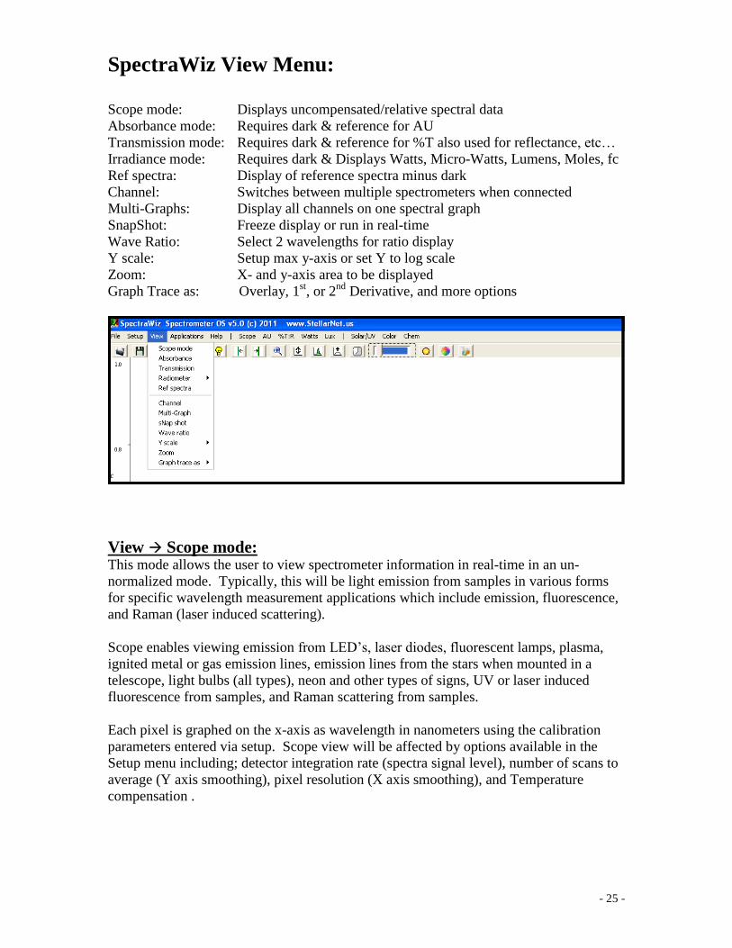
SpectraWiz View Menu:

Scope mode: Displays uncompensated/relative spectral data

Absorbance mode: Requires dark & reference for AU

Transmission mode: Requires dark & reference for %T also used for reflectance, etc…

Irradiance mode: Requires dark & Displays Watts, Micro-Watts, Lumens, Moles, fc

Ref spectra: Display of reference spectra minus dark

Channel: Switches between multiple spectrometers when connected

Multi-Graphs: Display all channels on one spectral graph

SnapShot: Freeze display or run in real-time

Wave Ratio: Select 2 wavelengths for ratio display

Y scale: Setup max y-axis or set Y to log scale

Zoom: X- and y-axis area to be displayed

Graph Trace as: Overlay, 1st, or 2

nd Derivative, and more options

View Scope mode: This mode allows the user to view spectrometer information in real-time in an un-

normalized mode. Typically, this will be light emission from samples in various forms

for specific wavelength measurement applications which include emission, fluorescence,

and Raman (laser induced scattering).

Scope enables viewing emission from LED’s, laser diodes, fluorescent lamps, plasma,

ignited metal or gas emission lines, emission lines from the stars when mounted in a

telescope, light bulbs (all types), neon and other types of signs, UV or laser induced

fluorescence from samples, and Raman scattering from samples.

Each pixel is graphed on the x-axis as wavelength in nanometers using the calibration

parameters entered via setup. Scope view will be affected by options available in the

Setup menu including; detector integration rate (spectra signal level), number of scans to

average (Y axis smoothing), pixel resolution (X axis smoothing), and Temperature

compensation .

- 26 -

View Absorbance: Displays the absorbance at pixel n using the current sample, reference, and dark data sets:

An = - log samplen - darkn

refn - darkn

View Transmission: (also used for Reflectance)

Displays percent transmission at pixel n using the current sample, reference, and dark

data sets:

Tn = samplen - darkn x 100

refn - darkn

Percent transmission is mathematically equivalent to percent reflection.

View Irradiance: Watts per square meter (W/m

2)

Micro-Watts per square centimeter (W/cm2)

Micro-moles per square meter per second (µmol/m2/s)

Lumen per square meter LUX (illuminance)

Lumen per square foot FC (foot-candles)

These SpectroRadiometer display modes provide a calibrated Y-axis. In order to use this

mode, the unit requires certain system calibration files to exist. Units ordered as a

SpectroRadiometer include calibration files for operation in this display mode. These

files are installed by clicking on the MyCal-nnnnn.exe file provided in the installation

CD.

To get moles, watts is multiplied by 0.00835 (an Einstein), which is a unit of energy in

photochemistry, that represents a dose of power that irradiates a sample for 1 second. An

Einstein is the amount of energy in 1 mole (Avogadro's number, 6.0222 x 1023

) of

photons. Another number displayed in this mode is PAR, which stands for

Photosynthetically Active Radiation, and is the integral of power from 400-700nm in

micro-moles per square meter per second. For Yield Photon Flux (YPF), the measured

photon flux (PF) is multiplied by the relative quantum efficiency (RQE) weighting

factors at each wavelength and then resulting values are summed from 300 to 800 nm.

For the illuminance display, the photopic response curve is used to formulate lumen per

meter2 which provides a LUX value.

The Irradiance calibration function located under the Apps menu can re-generate system

calibration files needed for operating in Irradiance view mode. This requires a calibrated

source lamp with its calibration data stored in a disk file. An example .irrad cal data (text

file) "NIST.icd" is provided. This file can be used to simulate an irradiance calibration

and produce the required system calibration files needed for selecting the Irradiance view

mode.

- 27 -

WARNING: the system irradiance cal files such as SW1.icf thru SW8.icf can be

easily overwritten.

Like most instruments, it is good practice to re-calibrate the SpectroRadiometer every

year.

Setup for Radiant and Luminous Flux Area in sq meter:

CR1: 11 mm diameter -> sq meter

IC2: 0.625 inch diameter -> sq meter

Other: User defined

Reset 1 sqm: Default area = 1 square meter

Radiant flux in watts = (irradiance) x (surface area)

Luminous Flux in lumen = (illuminance) x (surface area)

Setup range for watt and Rflux measurements:

Specify the start and end wavelengths for the range computation of the total power. The

default range is 400-700nm.

Setup Compensation for CR2-Aperture if it is being used.

View Ref spectra: Displays the reference and dark spectra previously saved as refn-darkn. This is useful for

troubleshooting absorbance or transmission applications. The Ref spectra must not be

clipped at its peaks, indicating an over-saturated reference.

View Channel: If multiple spectrometers are connected, this selection allows you to view data from the

different optical channels.

View Multi-Graphs: Allows display of multiple channels in a single graph. Re-select to turn this feature off.

The x-axis labeling can be switched by using view channel n. All active channels

will be displayed.

View SnapShot: Allows user to pause display. Re-selecting SnapShot when the display is paused will re-

start normal real-time display.

View Wave Ratio: Allows two wavelengths to be selected and displayed as a ratio in the upper left hand

corner. The default values 260 nm and 280 nm are used for DNA concentration

measurements.

- 28 -

View Y scale:

Set Max y:

Allows the user to specify the y-axis scale maximum value. Selecting the y-axis

rescale icon (left click) will override the Max y via auto scale. Entering a value of

0 will also perform an auto scale.

as Log:

Converts the y-axis into a Log10 scale. Re-selecting will convert back to a linear

y-axis. This can also be used to determine optical density of samples.

View Zoom: ON/OFF: This mode allows a selected region to be expanded into a full graph. This option will

work for any view mode. You are prompted for x-axis left and right wavelength and y-

axis top and bottom. Selecting a bottom as a negative value allows proper viewing for

differential displays. The Y zoom also can be enabled by right clicking on the Z button

for mouse xy zoom described below. The status panel on bottom right of graph will

show a "Z" when zoom is in effect. This reminds you that the x-axis has been zoomed.

You must re-select View Zoom to perform an "un-ZOOM." Click the Z button on the

toolbar, or click to the left side of the graph.

You may also use the mouse to zoom by clicking on the left region and holding the

button down while dragging (a box will appear to be expanding as you move) to the right

- 29 -

side of the region of interest. When you lift the left mouse button, the selected region will

appear as the full graph. This process can be repeated several times, each time refining

the area of interest smaller and smaller.

View Graph Trace as: Overlay or 1st /2

nd Derivative:

These options apply to any SpectraWiz view mode. Overlay allows the graph trace to

continuously plot without erasing the previous scan.

Using spectral derivatives eliminate problems with offset differences in samples. The

spectral data is converted to a spectral reference of itself similar to measuring rate of

change or acceleration. It is common practice to use spectral derivatives when generating

Neural Network training sets or performing PLS calibrations to determine species

concentrations.

To convert data to the 1st or 2

nd Derivative form, perform a View Graph Trace as

and select either the1st or 2

nd form. Click OK to confirm conversion.

In order to display derivatives properly, the graph needs to be centered at the zero line.

This can be performed by selecting the View Zoom and entering a smaller y-axis

range, such as 0.5 for the zoom y-axis top and -0.5 for the zoom y-axis bottom values.

To exit the derivative mode and return to the regular spectra, uncheck the type that was

selected.

- 30 -

SpectraWiz Applications Menu:

CIE Color Monitor: For SpectroColorimeter

ChemWiz Methods: For Chemical concentrations

Solar Monitor: For solar simulator classification

Irradiance Calibration: For SpectroRadiometer calibration

CIE Color Monitor: This SpectroColorimeter application provides a precise way to perform color

measurements using the basic principles and techniques defined by the International

Commission on Illumination (CIE).

If SpectraWiz is placed in the View Irradiance modes (for watts or lumens), then the

color of light is displayed using the xy chromaticity diagram and related dominant

wavelength. NOTE: the unit must first be calibrated to display these units properly. If

SpectraWiz is placed in the View transmission mode, the color of light is displayed

using CIELAB circular graph for a* and b*. The L* is the color lightness and is

displayed in a bar graph. This mode is used to measure color of reflected light.

The first set of values derived are known as tri-stimulus values which are proportions of

Red (700 nm), Green (546.1 nm), and Blue (435.8 nm). With these values, a uniform

color space is derived and known as the CIE 1976 (L* a* b*) color space or the CIELAB

color space. These values are pronounced L-star, a-star, and b-star. L* is the lightness

0…100, a* and b* are the color values from -60...+60.

CIELAB tolerancing is used to determine color differences known as Delta E. If two

colors are measured and the L*a*b* values are plugged into the following formula:

ΔE = (L1 - L2)2 + (a1 - a2)

2 + (b1 - b2)

2

The resulting number is referred to as Delta E (ΔE), or the color difference. Using this

value, you can calculate the difference between two colors, or alternatively between two

devices.

- 31 -

There are no hard and fast rules for ΔE accuracy requirements but there are some simple

guidelines. A ΔE ≤ 1.0 is assumed to be barely perceptible to a trained eye. For most

applications, an average ΔE ≥ 3 is considered two different colors.

Naturally, ΔE can be problematic to interpret. This is because of the difference in how the

eye sees and interprets color differences compared to how a device and software

interprets the color differences. A ΔE difference of 5 in the L* channel is probably less

noticeable and therefore less objectionable than the same amount of difference in the a*

or b* channels.

Additional tests will need to be performed to determine ΔE tolerance levels, but this will

be time well spent in the process of improving the overall quality of your final product.

CIELAB uses rectangular coordinates that are based on specific formulas using the tri-

stimulus values.

The L* a* b* values are computed in real time and are displayed graphically in the

circular color chart , which is updated several times per second, depending on the user

selected sample rate and sample averaging. If a fiber optic reflection probe is moved

across a spectral color chart, a data cursor can be seen to move in a circle around the

CIELAB color chart.

The application allows user selection of CIE Standard Illuminants A, B, C, D50, D55,

D65, D75 in addition to fluorescent lamps F1...F12. The CIELAB data is then

compensated from a table providing the relative spectral power distributions for the

selected illuminant.

Note: the default illuminant is D65 (daylight)

Prior to enabling the colorimeter, ensure that you have saved a dark reference and a white

reference (such as with the RS50 white standard) while in the Scope Mode.

This ensures that your spectrometer and reflectance probe/or integrating sphere, are

performing correctly with NO light and then with White light. For the best results when

using a reflectance probe, also use a fixture that holds the tip at the same distance and

angle from each sample (like the RPH reflectance probe holder).

When using the fiber probe, hold it at 45 degrees and ~ 1/4 inch away from the sample

surface. Make sure that the bell curve response viewed does not saturate at the top peak.

If it is oversaturated, then you should either adjust the detector time or adjust the sample

distance.

You may then enable the CIELAB Color Monitor application. The New Reference

button allows you to take a "standard white" re-reference at any time. This should give an

L value of 100 in the bar graph. Save sample allows you to rapidly record samples into a

"colordata.log" file for subsequent viewing or printing. The save standard allows a

particular sample to be loaded at a later time to compare with other samples. For Delta E

Values, a ColorData.log file allows the user to quickly save results for later viewing,

printing, or importing.

- 32 -

ChemWiz Methods: ChemWiz allows users to setup and use methods for predicting chemical concentrations.

To use this application for measuring liquid (or gas) chemicals, you will require

additional accessories with your configuration, such as a cuvette, a dip probe, or flow

cell. When a method is setup, a known maximum concentration is measured at a specific

wavelength and a calibration curve is then stored. The number of user configurable

methods is unlimited.

Once a method has been configured, it can be opened to operate in real-time. SpectraWiz

automatically sets the system parameters required by the specified method. This includes

detector integration time and all parameters found in the setup menu. When activated, it

will begin to display concentration values. It is important to setup for and press the Zero

Reference button. This requires the sample to contain the solvent solution or zero percent

concentration. It is a good idea to perform a Zero Reference as often as possible when a

second spectrometer channel is not available for automatic lamp drift correction. A

"ChemData.log" file allows users to quickly save samples for later viewing, printing, or

importing. For more information, please reference our ChemWiz tutorial.

Light Monitor (Solar + UV):

The Solar Match Monitor application calculates spectral irradiance for each 100nm bin

from 400-1100nm and compares the results to the ideal percent for each bin range per

IEC/JIS/ASTM. The proximity of the measured data to the ideal values results in

classification of the solar simulator lamp from A through D.

The Solar Match Monitor application is the default setting when the user has selected

View-> Irradiance-> Watts/m2 AND clicks on the yellow light bulb. The user can then go

to Applications->Click Light Monitor for display.

Save sample can be used to save each sample to the data log. In the Data Log, percentage

is provided for each wavelength range. Total power and Solar Class is provided for each

sample.

The UV Light Monitor measures UVabc regions below 400nm using U.S.FDA and

European health standards. The spectrometer must have a proper irradiance calibration

for the UV range from 200+ nm. This can be selected by doing the following: View->

Irradiance-> watts/m2 AND clicks on the yellow light bulb. The user can then go to

Applications->Click Light Monitor for display-> Select Solar Tab in left hand corner->

adjust setting to include appropriate health standard.

Short Wave UV

(UV-C)

Middle Wave UV

(UV-B)

Long Wave UV

(UV-A)

200 nm 280 nm 315 nm 400 nm

- 33 -

Computations are provided for UVa, UVb, and UVc in W/m2 including UVa/b ratio,

UVb and VIS-IR power, and time in minutes to the skin (Te) Erythema action as

prescribed by algorithms found on the U.S. FDA (Food and Drug Administrations)

website.

An override file can be created to limit low UV measurements to begin at 225nm or

250nm instead of 200nm. Create a file in the SpectraWiz directory named "UV250." or

UV230." To enable this feature, otherwise the default is 200nm.

U.S FDA display:

Irradiance values in watts per square meter

UVc=>200-280nm Uvb=>280-320nm UVa=>320-400nm

PowerUVb=>280-302nm PowerVIS-NIR=>400-850nm

Te minutes = weighted irradiance 250-400nm

Te weighting

------------

250-298nm -> 1

299-328nm -> 1 * power (0.114 * (302-nm))

329-400nm -> 1 * power (0.0161* (159-nm))

Spanish display

Effective Irradiance in watts per square meter

UVc=250-298nm, Uvb=299=328nm, UVa=329-400nm

Power<295=>200-294nm PowerVIS-NIR=>400-850nm

Te minutes = weighted effective irradiance 250-400nm

Te weighting

------------

250-298nm -> 1

299-328nm -> 1 * power (0.094 * (298-nm))

329-400nm -> 1 * power (0.015 * (139-nm))

A "UVdata.log" file allows users to quickly save monitor

display results for later viewing, printing, or importing.

Irradiance Calibration: This application allows users to perform irradiance calibrations in the field. It requires a

calibrated source lamp from 200-600nm or 300 to 1100nm. The calibration data for this

lamp needs to be in text file format with the wavelength and associated watt value on

each line, in 5nm increments.

You will be prompted to take a dark and then take a reading using the calibrated lamp

placed at a specified distance. Next the Irradiance Calibration Data is read from the file

- 34 -

that you have specified (such as text file NIST.icd). The new irradiance cal files are

generated (SW1.icf - for channel 1).

WARNING: Existing file(s) will be overwritten. Be sure to save files BEFORE

running.

For users who do not have a valid irradiance calibration, an example irrad cal data (text

file) "NIST.icd" is provided. This file can be used to simulate an irradiance calibration

and produce the required system calibration files needed for selecting the Irradiance view

mode. For this you may use any white light source that will produce a "bell shape"

curve.

WARNING: Existing "SW*.icf" irradiance cal file(s) will be overwritten. Be sure to save

files to preserve a previous "real" irradiance calibration.

NOTE: THIS IS NOT A VALID METHOD AND IS SUPPLIED FOR

DEMONSTRATION PURPOSES ONLY.

StellarNet provides an irradiance calibration service using an NIST calibration source

lamp (300-1100nm). Like most instruments, it is good practice to re-calibrate the system

after extended use.

Please Reference the Irradiance Calibration tutorial for more information.

- 35 -

Quick Guide for Transmission/Absorbance

Experiments

Using a Cuvette:

1) With the instrument and accessories connected, open the SpectraWiz program.

2) Enter the correct calibration coefficients and port/detector settings.

3) Enter into Scope Mode.

4) With the reference liquid in place (pure solvent in cuvette or empty cell), adjust the integration

time, number of scans to average, and XTiming resolution control.

5) With the light source off (or by blocking the light into the detector), take a DARK scan (left click

dark bulb icon).

6) Turn on the light source (or uncover the detector) and take a reference spectrum (left click light

bulb icon).

7) Enter into Transmission or Absorbance Mode and insert sample

8) Begin collecting data.

- 36 -

Using a Dip Probe:

1) With the instrument and accessories connected, open the SpectraWiz program.

2) Enter the correct calibration coefficients and port/detector settings.

3) Enter into Scope Mode.

4) Place the probe into the reference solution or by using air as the reference, adjust the integration

time, number of scans to average, and XTiming resolution control.

5) With the light source off (or by blocking the light into the detector), take a DARK scan (left click

dark bulb icon).

6) Turn on the light source (or uncover the detector) and take a reference spectrum (left click light

bulb icon).

7) Enter into Transmission Mode and insert the probe into the sample.

8) Begin collecting data.

- 37 -

Using a Transmission Fixture:

1) With the instrument and accessories connected, open the SpectraWiz program.

2) Enter the correct calibration coefficients and port/detector settings.

3) Enter into Scope Mode.

4) With the reference in place, adjust the integration time, number of scans to average, and XTiming

resolution control.

5) With the light source off (or by blocking the light into the detector), take a DARK scan (left click

dark bulb icon).

6) Turn on the light source (or uncover the detector) and take a reference spectrum (left click light

bulb icon).

7) Enter into Transmission Mode and the sample into the holder.

8) Begin collecting data.

- 38 -

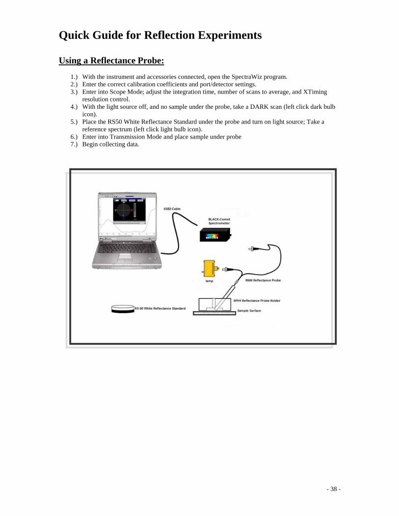
Quick Guide for Reflection Experiments

Using a Reflectance Probe:

1.) With the instrument and accessories connected, open the SpectraWiz program.

2.) Enter the correct calibration coefficients and port/detector settings.

3.) Enter into Scope Mode; adjust the integration time, number of scans to average, and XTiming

resolution control.

4.) With the light source off, and no sample under the probe, take a DARK scan (left click dark bulb

icon).

5.) Place the RS50 White Reflectance Standard under the probe and turn on light source; Take a

reference spectrum (left click light bulb icon).

6.) Enter into Transmission Mode and place sample under probe

7.) Begin collecting data.

- 39 -

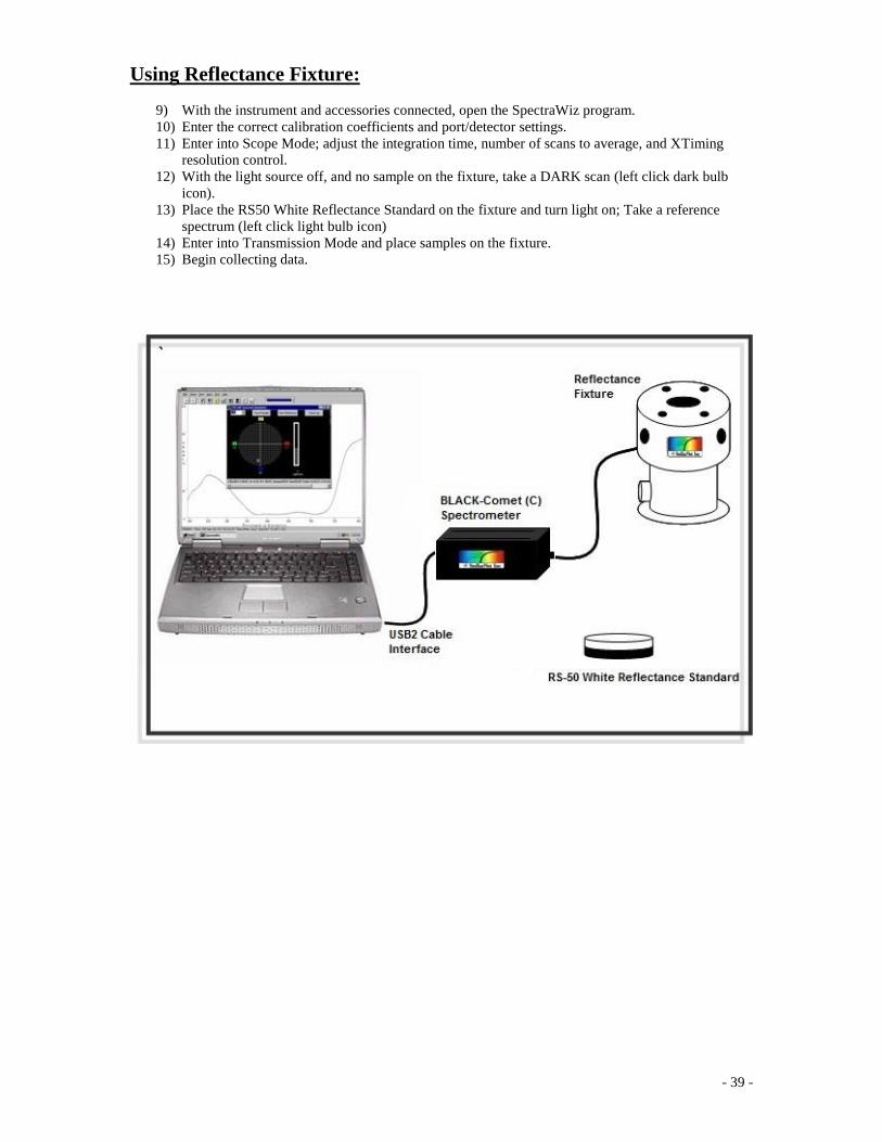
Using Reflectance Fixture:

9) With the instrument and accessories connected, open the SpectraWiz program.

10) Enter the correct calibration coefficients and port/detector settings.

11) Enter into Scope Mode; adjust the integration time, number of scans to average, and XTiming

resolution control.

12) With the light source off, and no sample on the fixture, take a DARK scan (left click dark bulb

icon).

13) Place the RS50 White Reflectance Standard on the fixture and turn light on; Take a reference

spectrum (left click light bulb icon)

14) Enter into Transmission Mode and place samples on the fixture.

15) Begin collecting data.

- 40 -

Tutorial: Configuring SpectraWiz as a Dual System (VIS+NIR):

1. Connect the VIS spectrometer to channel 1 on the computer and connect the NIR spectrometer

(typically an InGaAs or PDA unit) on channel 2.

2. Open SpectraWiz and go to Set-Up Unit Calibration Coefficients and enter 1 at the channel

prompt and enter the calibration coefficients for the VIS range spectrometer. Again, go to Set-Up

Unit Calibration Coefficients and enter 2 at the channel prompt and enter the calibration

coefficients for the NIR range spectrometer

3. Next, go to Set-Up Interface Port and Detector. Make sure that the USB2EPP is checked, and

also check the box next to the correct LT option.

NOTE: If you have both LT-12 and LT-14 or LT16 spectrometers, SpectraWiz will only allow

one to be checked-ALWAYS check the larger LT –(#) for dual systems.

4. For Channel 1 (VIS range) make sure the appropriate detector

type is selected (typically CCD 2048).

5. Select Channel 2 (NIR range) and either select InGaAs 512 or

InGaAs 1024, or another depending on which model is used.

These can be found on the label on the spectrometer bottom.

6. It will be necessary to exit SpectraWiz and restart the software

for the changes to take effect.

7. Before taking measurements, make sure that the correct

spectrometer is configured on the correct channel. This can be

done by illuminating each spectrometer with a white light

source (such as the SL1). If configured correctly, the

characteristic shape of each spectra will be seen:

NOTE: In Scope mode, the VIS channel (if REV6 or LT-12

electronics) will saturate at 4096 counts, while the NIR channel

(if LT-14 electronics or higher) will saturate at 16385 counts,

and all LT-16 electronics will saturate at 65,536 counts. This

will be seen whether or not the VIEW Multigraph function

is enabled.

8. The display can be modified so that the two spectra appear as

one, rather than overlapping where one unit ends and another begins. Go to Set-Up

Spectrometer Channels Multigraph Start-End. At the prompt enter 1 for Channel 1 and either

enter a value which you would like the first channel to start displaying (a value of 0 will default to

the spectrometers original starting wavelength). At the next prompt, enter the ending wavelength

for the first channel (again, a value of 0 will default to the spectrometers original ending

wavelength).

9. Once Channel 1 has been configured, enter 2 to perform the same set-up for the NIR channel or

enter 0 to exit the Multigraph Start-End mode.

- 41 -

Tutorial: Importing Data into Microsoft Excel

1) Open the Excel program

2) Go to Data Import External Data Import Data

3) Navigate to find your file. It will be necessary to change the type of file from

Files of type: All Data Sources over to Files of type: All Files in the drop

down menu.

4) Choose the delimited option at the prompt and press the Next button.

- 42 -

5) Select the following boxes to import the data: Tab, Space, Semicolon, and

Comma. Press the Next button.

6) Press the Finish button at the next prompt.

7) Select where the data is to be places and press the OK button.

8) From there the data can be manipulated in any fashion, as well as graphical

properties are needed. Consult the Help menu in the Excel program for

further information.

- 43 -

Tutorial: Irradiance Calibration using SpectraWiz® Software:

1) Ensure that all calibration coefficients (C1, C2, and C3) and interface port and detector

settings are correctly entered for the StellarNet spectrometer being used for irradiance

calibration (y-axis).

2) While in Scope mode, point the cosine receptor or integrating sphere at the calibrated light

source. If you are calibrating with the StellarNet model SL1-CAL calibration light source,

you may place the CR2 either inside of the nosecone (inserted) or at the tip of the nosecone

(at plane). Integrating spheres must be in the “at plane” position, as they cannot be inserted.

3) Adjust the integration time and averaging levels to maximize the light output of the source.

4) Select the Irradiance Application by going to Apps Radiometer Calibration.

5) You will be prompted to take a Dark Spectrum.

- 44 -

6) Block the light to the collection optics (or turn the light source off) and wait until you obtain a

flat line. Click YES to take a dark (background) spectrum.

7) The baseline will then drop to zero.

- 45 -

8) You will then be prompted to capture the spectrum of the calibrated light source, using the

integration time and other settings that were set in steps 2 and 3.

9) Capture the spectrum by unblocking the light so that you see the spectrum onscreen again and

click the YES button.

10) The software will then prompt you for the lamp calibration file, with the extension “.ICD.”

This file should be supplied with the lamp, giving a 2-column format of the wavelength and

- 46 -

compensated power values in (W/m2). For the StellarNet model SL1-CAL light source, you

will have one file for the inserted position and another for the at plane position.

NOTE: If you do not have a calibration file for the lamp, you can use the NIST.ICD file

contained in the SpectraWiz directory. This will give an approximate calibration for

demonstration purposes only.

11) The software will then prompt you to verify the format of the ICD file. For most calibrations

the format will be in W/m2, and you should select YES. If you have a file in another format,

click NO to step through the subsequent prompts and select the correct one.

- 47 -

12.) Depending on your spectrometer range, you might then be prompted if you would like to trim the

calibration at a certain ending wavelength. This is automatically selected by the calibration

software if a significant amount of noise is seen in the 1000-1100nm region.

- 48 -

13.) Another prompt will appear asking if a standard collection optic is installed. If you are not using

any filters or apertures to reduce the amount of light being collected, click YES. If a neutral

density filter or aperture has been installed, click NO and then enter the value of the filter/aperture

when prompted.

14.) You will then be asked if you would like to capture the entire spectrum of the calibration file used.

By clicking NO, you can specify a range (the starting and stopping wavelengths can be entered on

the next prompt).

- 49 -

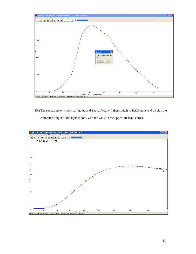
15.) The spectrometer is now calibrated and SpectraWiz will then switch to RAD mode and display the

calibrated output of the light source, with the value in the upper left-hand corner.

- 50 -

16.) It is recommended that you save a copy calibration files in the event it is overwritten. Do to this,

copy the files “sw.ini” and “SW1.icf” contained in the folder: C:\Program

Files\StellarNet\SpectraWiz.

- 51 -

Trouble-shooting:

Check our software download page often to get the most current software update. Before

contacting us, make sure that you have had time to read the supplied instruction manual

and view the Training Videos found on the CD-ROM or online. This will help you

become more familiar with the software. The best way to get assistance is to write a

detailed explanation of your problem and e-mail it to support@StellarNet.us. Be sure to

include the unit you are using (or supply the invoice number it was purchase under), and

what you are trying to measure. If possible, attach a screenshot of the item in question

and the file “sw.ini” found in the SpectraWiz directory.

Symptom Solution I don’t see a signal. Ensure coefficients and interface parameters

have been entered correctly.

Check to see if unit has power (green LED is

on).

Inspect fiber optic cable to make sure it is not

broken.

I get the error message “USB device not

present” and/or “Scan Timeout.”

Check to see if unit has power.

Check to see if the cables are listed in the

Windows Device Manager under USBDEV.

Check to see if USB cable is firmly inserted

in back of unit and USB port of computer.

Close SpectraWiz and perform a reboot of

USB driver using the following steps: 1)

Unplug power cord from unit. 2) Unplug

USB2 cable from unit. 3) Unplug USB2

cable from computer. 4) Plug USB2 cable

into unit. 5) Plug power supply into unit. 6)

Plug USB2 cable into computer.

The software locks up. Check to see if multiple channels are

configured: Under Set-up- Unit Calibration

Coefficients. Enter 2 for 2nd channel and

press 0 for the first coefficient.

Under Set-up - Interface port and detector,

disable channels 2 and above by making sure

no other detector type is checked.

The green LED on my spectrometer is

not on.

Check to see if sufficient power is supplied to

unit (+5V DC).

Make sure no other voltage has been applied

to unit (such as the +12V DC for light

sources).

- 52 -

I get the following error: “I/O 32.” Delete the swref1 and swdark files from the

SpectraWiz directory.

My unit is not displaying the correct

wavelength range.

Ensure coefficients and interface parameters

have been entered correctly.

Make sure spectrometer is not running off of

computer power (via USB cable).

Turn zoom off by left-clicking to the left of

the y-axis.

Uncheck the Multiplexer option: Set-up

-Spectrometer channels -Fiber Optic

Multiplexer.

I get a “Range Error” when in

Irradiance mode.

Back away the unit from the light source (if

possible).

Install a calibrated aperture.

Decrease the integration time.

My measurements don’t look right

(using the R400 reflectance probe).

Insert the end of the y-fiber with 6 fibers

bundled into the light source. Insert the other

end into the spectrometer (to get the most

amount of light onto the sample).

Block any overhead lights from the probe

Make sure the reference is not oversaturated.

I get the following error “Reference

Oversaturated at xxx nm.”

Decrease the integration time

Back the light source away from the unit (if

possible).

I’m having difficulty with my port

settings.

We no longer support devices using parallel

ports. Purchase our USB2EPP cable to run the

spectrometer from USB-1 or USB-2 ports.

Is my Spectrometer calibrated for

Irradiance measurements?

A 3.5” floppy disk is sent with all calibrated

units. Check the computer for a file called

MyCal (with your unit’s serial number in the

file name).

I get the error message “No WAV device

found.”

In the SpectraWiz directory double-click the

file: NOSOUND.bat.

Delete the following files: swdo.wax and

swds.wax

Contact support@StellarNet.us with your unit’s serial number.

- 53 -