University of Illinois at Urbana-Champaign

Air Conditioning and Refrigeration Center A National Science Foundation/University Cooperative Research Center

Steady-State Performance of a Domestic Refrigerator/Freezer Using R12 and R134a

D. M. Staley, C. W. Bullard, and R. R. Crawford

ACRC TR-22 June 1992

For additional information: Air Conditioning and Refrigeration Center University of Illinois Mechanical & Industrial Engineering Dept. 1206 West Green Street Urbana, IL 61801 Prepared as part of ACRC Project 12 Analysis of Refrigerator-Freezer Systems (217) 333-3115 C. W. Bullard, Principal Investigator

ii

The Air Conditioning and Refrigeration Center was founded in 1988 with a grant from the estate of Richard W. Kritzer, the founder of Peerless of America Inc. A State of Illinois Technology Challenge Grant helped build the laboratory facilities. The ACRC receives continuing support from the Richard W. Kritzer Endowment and the National Science Foundation. The following organizations have also become sponsors of the Center. Acustar Division of Chrysler Allied-Signal, Inc. Amana Refrigeration, Inc. Bergstrom Manufacturing Co. Caterpillar, Inc. E. I. du Pont de Nemours & Co. Electric Power Research Institute Ford Motor Company General Electric Company Harrison Division of GM ICI Americas, Inc. Johnson Controls, Inc. Modine Manufacturing Co. Peerless of America, Inc. Environmental Protection Agency U. S. Army CERL Whirlpool Corporation For additional information: Air Conditioning & Refrigeration Center Mechanical & Industrial Engineering Dept. University of Illinois 1206 West Green Street Urbana, IL 61801 217 333 3115

iii

Abstract

This paper develops a steady-state system design model for a standard 18 ft3 refrigerator/freezer. Models for

the compressor, condenser, evaporator, and suction line interchanger are considered. Experimental data for both R12

and R134a are used as a basis to calibrate the models and as a basis of comparison of model validity for different

refrigerants. For each model, a set of independent model parameters are determined from the experimental data using

optimization methods. For the heat exchangers both constant conductance and variable conductance models are

considered. Lastly, a preliminary overview is made of the applicability of a quasi-steady refrigerator model for use in

describing normal cycling operation of a refrigerator/freezer.

iv

Table of Contents

Page

Abstract.........................................................................................................................................iii

List of Figures ........................................................................................................................... vii

List of Tables .............................................................................................................................. ix

Chapter 1: Introduction ............................................................................................................ 1

Chapter 2: Literature Review .................................................................................................. 2

2.1 Purpose .................................................................................................................................2

2.2 Steady-State Simulation Models...........................................................................................2

2.3 Quasi -Steady Models.............................................................................................................3

2.4 Transient Models...................................................................................................................4

2.5 Alternate Refrigerants ...........................................................................................................4

2.6 Implications for Current Study...............................................................................................6

Chapter 3: Instrumentation...................................................................................................... 7

3.1 Refrigerator Instrumentation .................................................................................................7

3.2 Heater System ..................................................................................................................... 10

Chapter 4: Experimental Procedure....................................................................................17

4.1 Refrigerator Testing............................................................................................................. 17

4.2 R134a Refrigerator Conversion............................................................................................ 18

Chapter 5: Overview of Parameter Estimation .................................................................20

5.1 Refrigerator State Points..................................................................................................... 20

5.2 Optimization Techniques..................................................................................................... 20

5.3 Experimental Uncertainty Analysis...................................................................................... 23

Chapter 6: Compressor Parameter Estimation ................................................................27

6.1 Overview ............................................................................................................................. 27

6.2 R12 Compressor Maps ......................................................................................................... 27

6.3 Volumetric Efficiency Approach for the R12 Compressor..................................................... 30

6.4 Volumetric Efficiency Curve Fits for the R134a Compressor ................................................ 34

6.5 Compressor Shell Heat Transfer.......................................................................................... 37

6.6 Conclusions......................................................................................................................... 40

Chapter 7: Condenser Parameter Estimation...................................................................42

v

7.1 Overview ............................................................................................................................. 42

7.2 Condenser Volumetric Flow Rate ........................................................................................ 43

7.3 Constant Conductance Model.............................................................................................. 46

7.4 Variable Conductance Model .............................................................................................. 51

7.5 Contour Plots....................................................................................................................... 53

7.6 Conclusions......................................................................................................................... 54

Chapter 8: Suction Line Heat Exchanger Parameter Estimation ................................56

8.1 Overview ............................................................................................................................. 56

8.2 Constant Effectiveness Model .............................................................................................. 56

8.3 Constant UA Model .............................................................................................................. 59

8.4 Conclusions......................................................................................................................... 62

Chapter 9: Evaporator Parameter Estimation...................................................................64

9.1 Overview ............................................................................................................................. 64

9.2 Evaporator Volumetric Flow Rate........................................................................................ 65

9.3 Constant Conductance Model.............................................................................................. 69

9.4 Variable Conductance Model .............................................................................................. 80

9.5 Conclusions......................................................................................................................... 81

Chapter 10: Conclusions and Recommendations..........................................................83

List of References ....................................................................................................................85

Appendix A: Performance Degradation of Domestic Refrigerators during Cyclic Operation....................................................................................................................................87

A.1 Overview............................................................................................................................. 87

A.2 Cycling Performance in Heat Pumps and Air-Conditioning Equipment............................... 87

A.3. Comparison of Steady-State Performance and a "Snapshot" of Cycling Performance ...... 88

A.4 Refrigerant Charge Migration from the Condenser............................................................. 92

A.5 Comparison of Steady-State and Cyclic Performance Over an Entire Cycle....................... 99

A.6 Conclusions....................................................................................................................... 101

Appendix B: Reverse Heat Leak Tests.............................................................................103

Appendix C: Refrigerator Charge Tests...........................................................................107

Appendix D: Experimental Uncertainty Analysis...........................................................112

Temperature Measurement Uncertainty.................................................................................. 112

Pressure Transducer Uncertainties......................................................................................... 112

vi

Watt Transducer Uncertainty................................................................................................... 113

Uncertainty in Enthalpy Calculations ...................................................................................... 114

Refrigerant Mass Flow Rate Uncertainties.............................................................................. 115

Condenser Volumetric Flow Rate Uncertainty ........................................................................ 115

Condenser Heat Transfer & Conductance Uncertainties.......................................................... 116

Compressor Shell Heat Transfer Uncertainties........................................................................ 122

Interchanger Uncertainties...................................................................................................... 125

Evaporator Volumetric Air Flow Rate Uncertainty................................................................... 129

Evaporator Conductances and Heat Transfer Uncertainties.................................................... 133

Appendix E: Program Listings ...........................................................................................137

Appendix F: Experimental Data..........................................................................................157

R12 – Data ............................................................................................................................... 157

R134a - Data ............................................................................................................................ 162

Data Acquisition Channel Numbers......................................................................................... 167

Appendix G: Film Coefficients ............................................................................................168

G.1 Condenser Film Coefficients............................................................................................. 168

G.2 Evaporator Film Coefficients............................................................................................. 171

vii

List of Figures

Page

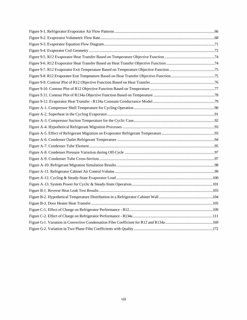
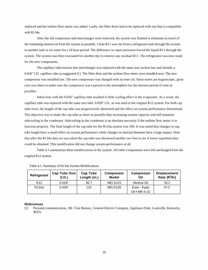
Figure 3-1. Refrigerant Side Pressure and Temperature Measurement Locations ..................................................................7 Figure 3-2. Immersion Thermocouple and Pressure Tap Mounting Technique......................................................................8 Figure 3-3. Air Side Thermocouple Layout ...................................................................................................................................9 Figure 3-4. Heater System..............................................................................................................................................................11 Figure 3-5. Heater System Circuit..................................................................................................................................................12 Figure 3-6. Heater System Control Signals ..................................................................................................................................13 Figure 3-7. Power Verification Circuit ...........................................................................................................................................14 Figure 5-1. Refrigerator/Freezer State Point Diagram.................................................................................................................20 Figure 5-2. Contour Plot of a Hypothetical Objective Function...............................................................................................23 Figure 5-3. Temperature Measurement Uncertainty ..................................................................................................................24 Figure 6-1. Biquadratic Curve Fit of Compressor Calorimeter Mass Flow Data ....................................................................29 Figure 6-2. Biquadratic Curve Fit of Compressor Calorimeter Power Data.............................................................................29 Figure 6-3. Comparison of R12 Data Set to Compressor Map Range......................................................................................30 Figure 6-4. Volumetric Efficiency Curve for the R12 Compressor............................................................................................31 Figure 6-5. Isentropic Compressor Efficiency Curve for the R12 Compressor.......................................................................32 Figure 6-6. R12 Mass Flow Rate Curve Fit Using Volumetric Efficiency...............................................................................33 Figure 6-7. R12 Compressor Power Curve Fit Using Isentropic Efficiency ............................................................................33 Figure 6-8. Volumetric Efficiency for R134a Compressor..........................................................................................................34 Figure 6-9. Isentropic Efficiency for R134a Compressor...........................................................................................................35 Figure 6-10. R134a Mass Flow Rate Curve Fit Using Volumetric Efficiency..........................................................................36 Figure 6-11. R134a Compressor Power Curve Fit Using Isentropic Efficiency ......................................................................36 Figure 6-12. Convective Film Coefficient for the R12 Compressor..........................................................................................38 Figure 6-13. R12 Compressor Shell Heat Transfer......................................................................................................................39 Figure 6-14. Convective Film Coefficient for R134a Compressor.............................................................................................39 Figure 6-15. R134a Compressor Shell Heat Transfer..................................................................................................................40 Figure 7-1. Refrigerator Condenser/Compressor Geometry ......................................................................................................44 Figure 7-2. Condenser Volumetric Flow Rate..............................................................................................................................45 Figure 7-3. Condenser Heat Transfer - R12 Constant Conductance Model...........................................................................51 Figure 7-4. Condenser Heat Transfer - R134a Constant Conductance Model.......................................................................51 Figure 7-5. R134a Squared Errors Plotted as a Function of Udesup and U2ph.............................................................................54 Figure 7-6. R134a Squared Errors Plotted as a Function of Udesup and Usub.............................................................................54 Figure 8-1. Idealized Suction Line Heat Exchanger....................................................................................................................56 Figure 8-2. Interchanger Effectiveness - R12 data......................................................................................................................57 Figure 8-3. Interchanger Effectiveness - R134a ..........................................................................................................................58 Figure 8-4. R12 Interchanger Heat Transfer - Constant Effectiveness Model.......................................................................58 Figure 8-5. R134a Interchanger Heat Transfer - Constant Effectiveness Model...................................................................59 Figure 8-6. R12 Interchanger Heat Transfer - Constant UA Model.........................................................................................61 Figure 8-7. R134a Interchanger Heat Transfer - Constant UA Model.....................................................................................62

viii

Figure 9-1. Refrigerator Evaporator Air Flow Patterns ..............................................................................................................66 Figure 9-2. Evaporator Volumetric Flow Rate..............................................................................................................................68 Figure 9-3. Evaporator Equation Flow Diagram..........................................................................................................................71 Figure 9-4. Evaporator Coil Geometry ..........................................................................................................................................72 Figure 9-5. R12 Evaporator Heat Transfer Based on Temperature Objective Function .......................................................74 Figure 9-6. R12 Evaporator Heat Transfer Based on Heat Transfer Objective Function .....................................................74 Figure 9-7. R12 Evaporator Exit Temperature Based on Temperature Objective Function..................................................75 Figure 9-8. R12 Evaporator Exit Temperature Based on Heat Transfer Objective Function................................................75 Figure 9-9. Contour Plot of R12 Objective Function Based on Heat Transfer.......................................................................76 Figure 9-10. Contour Plot of R12 Objective Function Based on Temperature .......................................................................77 Figure 9.11. Contour Plot of R134a Objective Function Based on Temperature ...................................................................78 Figure 9-12. Evaporator Heat Transfer - R134a Constant Conductance Model....................................................................79 Figure A-1. Compressor Shell Temperature for Cycling Operation.........................................................................................90 Figure A-2. Superheat in the Cycling Evaporator......................................................................................................................91 Figure A-3. Compressor Suction Temperature for the Cyclic Case.........................................................................................92 Figure A-4. Hypothetical Refrigerant Migration Processes .....................................................................................................93 Figure A-5. Effect of Refrigerant Migration on Evaporator Refrigerant Temperature ..........................................................93 Figure A-6. Condenser Outlet Refrigerant Temperature ...........................................................................................................94 Figure A-7. Condenser Tube Element..........................................................................................................................................95 Figure A-8. Condenser Pressure Variation during Off-Cycle ...................................................................................................97 Figure A-9. Condenser Tube Cross-Section...............................................................................................................................97 Figure A-10. Refrigerant Migration Simulation Results............................................................................................................98 Figure A-11. Refrigerator Cabinet Air Control Volume..............................................................................................................99 Figure A-12. Cycling & Steady-State Evaporator Load ..........................................................................................................100 Figure A-13. System Power for Cyclic & Steady-State Operation.........................................................................................101 Figure B-1. Reverse Heat Leak Test Results .............................................................................................................................103 Figure B-2. Hypothetical Temperature Distribution in a Refrigerator Cabinet Wall ...........................................................104 Figure B-3. Door Heater Heat Transfer......................................................................................................................................105 Figure C-1. Effect of Charge on Refrigerator Performance - R12............................................................................................109 Figure C-2. Effect of Charge on Refrigerator Performance - R134a ........................................................................................111 Figure G-1. Variation in Convective Condensation Film Coefficient for R12 and R134a ....................................................169 Figure G-2. Variation in Two Phase Film Coefficients with Quality.......................................................................................172

ix

List of Tables

Page

Table 3.1. Watt Transducer Verification Data.............................................................................................................................15 Table 3.2. Heater System Controller Settings..............................................................................................................................16 Table 4.1. Summary of R134a System Modifications.................................................................................................................19 Table 6.1. R12 Compressor Calorimeter Data ..............................................................................................................................28 Table 7.1. Constant Conductance Model Parameters................................................................................................................49 Table 7.2. Objective Function Sensitivities - Variable Conductance Model..........................................................................53 Table 8.1. Constant Effectiveness Model Results .....................................................................................................................57 Table 8.2. Constant Overall Heat Transfer Coefficient Model Results ...................................................................................60 Table 8.3. Internal Suction Line Convective Film Coefficients.................................................................................................60 Table 9.1. Evaporator Volumetric Flow Rate Results .................................................................................................................68 Table 9.2. Constant Conductance Model Results ......................................................................................................................73 Table A.1. Steady-State and Instantaneous Cyclic Performance ............................................................................................89 Table A.2. Steady-State and Average Cyclic Performance.....................................................................................................101 Table B.1. Reverse Heat Leak Data Summary ...........................................................................................................................104 Table B.2. Thermal Resistances in Refrigerator Cabinet .........................................................................................................104 Table C.1. Refrigerant Charge Tests Data Summary ................................................................................................................108 Table C.2. Coefficients for Curve Fits of Charge Data.............................................................................................................109 Table C.3. System Pressure Losses Before and After Additional Instrumentation Installation.......................................110 Table C.4. Predicted Effect of System Pressure Losses on Performance..............................................................................110 Table G.1. Condenser Fin Effectiveness Calculation Results.................................................................................................170 Table G.2. Theoretical Condenser Conductances ....................................................................................................................171 Table G.3. Evaporator Fin Effectiveness Calculation Results ................................................................................................173 Table G.4. Theoretical Evaporator Conductances....................................................................................................................173

1

Chapter 1: Introduction

Since the original discovery that chlorofluorocarbons destroy ozone [1], the European community and 24

nations have signed the Montreal Protocol [2] which contains the framework for the reduction and elimination of

CFC's. Concurrently in the U.S., Congress enacted legislation [3] that sets minimum energy efficiency standards for

household appliances. Further, recent measurements [4] indicate that the depletion of ozone may be worse than

originally thought. This has increased the pressure to accelerate the phase out time tables for R12. As a result, the

refrigeration industry and the appliance industry in particular must bear the double burden of eliminating the use of

R12, a CFC, and at the same time increase the efficiency of their appliances.

The need to evaluate and test alternative refrigerants in domestic refrigerators is immediate. The original

hope for a drop-in replacement has disappeared. At the present time it appears that R134a will most likely be the

chosen replacement for R12. However, this is by no means the final solution. As a result, the evaluation of

alternatives continues.

As part of this effort, a good refrigerator simulation model can be used to make relative comparisons among

different replacement candidates. Many more possible alternatives can be evaluated than either time or money would

allow for testing. The best candidates can then be chosen for testing. Further for the model to be useful, it should be

able to handle different refrigerants without complication.

The primary purpose of the work presented here is to develop a steady-state system design model, as well

as component models, for a standard 18 ft3 top-mount domestic refrigerator/freezer and evaluate how the models must

be adapted to accurately predict refrigerator performance with alternative refrigerants. In the process experimental

data will be collected for both R12 and R134a to provide a data base for analysis. Further, methods for obtaining

system parameters such as volumetric flow rates etc. will also be presented. Once the models are validated for

different refrigerants, they then can be used as building blocks for the development of a system simulation model for

alternative refrigerants. A simulation model consists of the same component models as a design model, plus models

of the capillary tube and the charge inventory.

Chapter 2 reviews some of the recent work on refrigerator modeling and alternative refrigerants. Chapters 3

and 4 describe the experimental instrumentation and procedures used in creating the R12 and R134a data bases.

Chapter 5 introduces some of the topics common to all the component chapters. Chapters 6 through 9 present the

results for the components studied and Chapter 10 discusses conclusions and recommendations for future research.

Appendix A summarizes some initial analysis of normal cycling operation of a domestic refrigerator. The applicability

of a quasi-steady state model is investigated.

References [1] Molina, M.J. and F.S. Rowland. 1974. "Stratospheric Sink for Chlorofluoromethanes: Chlorine Atom Catalyzed

Destruction of Ozone,” Nature 249: pp. 810 to 812.

[2] United Nations Environmental Programme. 1987. Montreal protocol on substances that deplete the ozone layer. Final act., New York: United Nations.

[3] NAECA. 1987. Public law 100-12, March 17.

[4] Science. v. 254, no. 5032, 1991.

2

Chapter 2: Literature Review

2.1 Purpose The intent of this literature review is to examine some of the recent work on the modeling of

refrigerator/freezers. It builds on the review conducted by Reeves [1] which contains additional references. This

review also covers some of the work on alternative refrigerants for use in domestic refrigerators.

2.2 Steady-State Simulation Models Rogers and Tree [2] present an algebraic model for each component in a refrigerator/freezer and combine

them to form a steady-state system simulation model. Their model for the compressor considers both heat transfer

within the compressor and from the compressor shell. For the heat transfer from the compressor shell, a three zone

model consisting of the top, side, and bottom of the compressor is developed. An overall heat transfer coefficient is

calculated from internal and external film coefficients for each section. No mention is made of how these heat transfer

coefficients were determined.

Given the shell heat transfer, the heat transfer from the motor windings and the inlet suction gas

temperature, the inlet temperature to the compressor cylinder is determined. The compression process is treated as a

polytropic compression. From this expression the discharge temperature from the compressor cylinder is determined.

With the exit temperature from the compressor cylinder known, the heat transfer from the discharge gas tube

to the surrounding suction gas is determined. This heat transfer process was modeled as a simple counterflow heat

exchanger. After considering the heat transfer to the suction gas, the discharge temperature from the compressor is

now known.

For the mass flow rate, a volumetric efficiency equation is used. Their expression is exactly the same as

Equation 6.4 in Chapter 6. No mention is made of how the volumetric efficiency or polytropic exponent etc. were

determined. However, comparison with experimental results showed the measured mass flow rate to agree within

±3%.

The relationship between the pressure difference across the capillary tube and the mass flow rate is

developed from the homogeneous model for two phase flow [3]. Comparisons with experimental data for a real

capillary tube/suction line interchanger showed good agreement for cases where subcooled liquid entered the cap

tube. The model did not do a very good job when the inlet was two phase.

The models for the heat exchangers are based on effectiveness-NTU relations for each zone similar to those

in Chapters 7 and 9. Equations were written for each zone in each heat exchanger, i.e. desuperheating, two phase,

subcooled and superheated. However, only overall heat transfer coefficients or UA's were considered. No attempt

was made to separate the areas from the conductances.

The above component models were combined into a system model. The capacity of the evaporator as well

as the evaporating temperature are inputs to the model. Further, the power input to the compressor must be given. No

mention is made of the existence of a condenser or evaporator fan. The outputs from the model are the mass flow rate,

the condensing pressure, the UA's for each section of the the heat exchangers, and the evaporator outlet

temperature.

3

The need to input important parameters such as evaporator heat transfer limits the usefulness of this model.

It is not a design model where the evaporator capacity and the evaporator temperature would be outputs and

parameters such as the ambient temperature would be inputs.

2.3 Quasi -Steady Models Hara et. al. [4] applied a quasi-steady model to simulate the transient response of the cooling capacity of a

refrigerator/freezer from startup to a steady-state condition. No attempt was made to develop component models.

Rather, the standard vapor compression cycle diagram with no pressure drops in the heat exchangers was used as a

starting point. Their diagram was based on the assumptions that the compressor suction temperature was equal to

the ambient temperature and the evaporator exit temperature was 10°C lower. The exit quality from the condenser and

the condensing temperature were also fixed.

A simple first order lumped capacitance model was written for each compartment of the refrigerator. The

difference between the specified evaporator load and the sum of the cabinet load plus evaporator fan power

determined the response of the system. The cabinet load was calculated from a finite element model of all the exterior

walls.

The refrigerator studied by Hara et. al. had a convectively cooled condenser. The condenser tubing was run

along the inside of the sheet metal of the exterior walls. Essentially the same configuration is used in many domestic

refrigerators to prevent moisture condensation. As for the cabinet walls a finite element program was written to

determine the amount of heat from the condenser tubing that flows back into the cabinet. This heat transfer was also

measured experimentally by placing small heaters inside the condenser tubing. When the surface temperature of the

exterior wall adjacent to a heater tube was equal to ambient conditions, the power input to the heater is equal the heat

transfer into the refrigerator cabinet. It was found that this heat transfer was of the order of 10 to 15 W.

Sugalski, Jung, and Radermacher [5] developed a quasi-transient model that simulates the normal cycling

operation of a refrigerator/freezer. They assume that the temperatures, pressures, etc. in the system change slowly

enough that thermal equilibrium exists in the system. This model is a combination of a purely steady-state mo del like

Rogers and Tree's and a fully transient model like Xiuling's. However, the model does not have the capability of

simulating start up transients.

As a starting point, a steady-state model was produced. The model did not include a mass flow/pressure

drop equation for the cap tube or consider refrigerant inventory. As a result the amount of subcooling at the

condenser outlet and the amount of superheat at the evaporator outlet must be specified by the user. Effectiveness-

NTU relations were used to model the heat exchangers. No mention is made of whether multiple zones are considered.

It appears that they were not considered because the user only specifies one overall heat transfer coefficient for each

heat exchanger. The user must also specify the volumetric flow rates across the coils.

The compressor model follows the same general approach as Rogers and Tree. It requires the user to input a

long list of parameters including a polytropic coefficient, isentropic efficiency, motor efficiency, displacement volume

etc, to specify the performance of the compressor. The model for the suction line heat exchanger is exactly the same

as the constant UA model given in Chapter 8 of this report. The outputs from this model include the compressor

power, the mass flow rate, and the evaporator load.

4

This refrigerant system model is combined with a cabinet model to produce the final quasi-steady state

model. The cabinet model is based on a steady-state UA∆T approach where the overall heat transfer coefficient was

determined from theoretical inside and outside film coefficients and the wall resistance. The cabinet model also

considers cabinet heat storage. A finite element program was written to investigate the shape the temperature profile

in the cabinet wall as the temperature inside the refrigerator varied. It was found that the temperature profile remained

essentially linear even when the internal compartment temperatures started at ambient conditions. As a result, the

cabinet heat storage term could be easily calculated.

The model was run with both R12 and R22/R142b mixture. The results showed that a R22/R142b mixture

required about 4.5% less energy a day than R12. Experimental measurements confirmed that the energy consumption

was less but only by 2 to 3%. It is not stated if in running the models any consideration was given of the effect of the

different fluids on the UA's of the heat exchangers or if any corrections were made.

2.4 Transient Models Xiuling et. al. [6] developed a first order fully transient model for a refrigerator/freezer. Basic continuity and

energy equations containing refrigerant mass storage and energy storage terms were written for both the evaporator

and the condenser. A linear quality model was assumed for the two phase sections and the desuperheating section in

the condenser was neglected. Both convective heat transfer and radiative heat transfer is accounted for on the air

side of the coils.

The mass flow rate through the compressor cylinder was determined from a volumetric efficiency equation.

The compressor power was calculated assuming a polytropic compression process. Equations were also written

containing refrigerant mass storage and energy storage terms to account for the thermal mass of the compressor. No

mention is made of how the capacitance for the compressor was determined.

The model for the capillary tube was restricted to the adiabatic case and only considers the condition where

the inlet refrigerant is subcooled. Mass flow and pressure drop equations were developed for both the subcooled

and two phase sections. The equation for the two phase section assumed that the two phase flow is compressible

Fanno Flow.

The system of differential equations was solved using Euler's method with interval-halving to simulate the

startup of a refrigerator. Comparison of the simulation results with the refrigerator studied showed good agreement

for pressures and temperatures and only fair agreement for power input. The mass flow rate did not agree very well

during the initial startup of the refrigerator; only after approximately a minute did the predicted and measured flow

rates agree.

2.5 Alternate Refrigerants Vineyard [7] screened many different possible replacements for R12 in domestic refrigerators based on

ozone depletion potential, global warming potential, predicted cycle efficiency and safety concerns such as

flammability. A set of three pure refrigerants, R134a, R134, R152a, one binary blend R134a/R152a, and two ternary

blends, R22/R152a/R124 and R134a/R152a/R124 were chosen for testing based on these criteria. For each refrigerant

the compressor was replaced to adjust for different required volumetric capacities. One of three capillary tubes were

available for use. The final selection of a capillary tube was based on which one gave the best performance.

5

The results for all the pure components showed a higher daily energy consumption compared to R12. R152a

was the best performer with an increase in daily energy consumption of of 3% after being corrected for compressor

efficiency. However, it has the major drawback of being flammable. R134a and R-134 had the same energy

consumption increase of 5.5%. It was found that lower viscosity oil improved the efficiency of R134a. This is effect

could not be solely accounted for by a decrease in compressor losses. It was speculated that higher refrigerant/oil

miscibility may improve evaporator heat transfer and account for the difference.

Camporese et. al. [8] compared the performance of R134a and the flammable refrigerants R152a, RC270, DME,

R290-R134a and R290-RC270 to R12. Their tests were strictly drop-in replacement tests. No modifications were made

to the compressor or the capillary tube. However, the results are consistent with Vineyard's. R152a showed a 2%

increase in daily energy consumption and R134a showed a 4.3% increase over R12. The refrigerants DME and RC270

did worse than R134a. As a result of their flammability, the authors considered that these refrigerants were not worth

further investigation. The refrigerant mixture R290-RC270 had an equivalent performance to R12 but has a low

flammability limit. The remaining mixture R290-R134a with 20% propane showed better performance than R12 but still

contains a flammable component.

Pereira, Neto, and Thiessen [9] tested both R12 and R134a in a 420 dm3 top-mount refrigerator. The R12

compressor was replaced with a compressor that had nearly the same refrigerating capacity and exactly the same

power requirement as the R12 compressor at the same rating conditions. The capillary tube was also replaced and

optimized to give equivalent performance to the R12 refrigerator. With these changes it was found that the R134a

system consumed about 2.4% more energy than the R12 system. However, there is a good deal of uncertainty in the

measurements and the comparison is more qualitative than quantitative. The authors suggest that it may be possible

to increase the efficiency of the R134a refrigerator by reoptimizing the heat exchangers. Note that the same

evaporator and condenser were used for both tests.

He, Spindler, Jung, and Radermacher [10], tested mixtures of R22/R142b as a possible replacement for R12.

They started with a standard 18 ft3 top-mount refrigerator. Extensive modifications were made to the heat exchangers

to make them counterflow. This was done to take advantage of the temperature glide inherent in NARMs. The

capillary tube was also reoptimized for each refrigerant mixture tested to give the same subcooling at the condenser

exit and superheat at the evaporator outlet as for the R12 case.

For the initial tests, the compressor was the same as that used in the R12 tests. A 0.55/0.45 mixture of

R22/R142b was chosen for this test because theoretical calculations revealed the mixture had the same volumetric

capacity as R12. In this way the compressor run times would be nearly equal making the comparison between the

mixture and R12 more fair. Even though simulation results showed a 3% increase in COP, the real system with various

mixture concentrations was always 3 to 4% worse. However, the replacement of the mineral oil in the compressor with

the same viscosity alkybenzene showed a dramatic increase in performance for the R22/R142b mixtures.

Further tests revealed the best mixture to have an R22 mass fraction of 0.52. The daily energy consumption

for this mixture was 1.9 to 3.5% lower than that for R12. The authors speculate that the better performance is the

result of a larger latent heat of evaporation for the mixture. However, the drawback of this mixture is the fact that

6

R142b is flammable. Since R22 is the more volatile component, the potential for leaks causing an increase in R142b

concentration is a concern.

2.6 Implications for Current Study The work considered here is an extension of the work by Rogers and Tree and the steady-state part of the

work by Sugalski, Jung, and Radermacher. Emphasis will be placed on the heat exchangers. Rather than consider

overall heat transfer coefficients for each zone in the heat exchangers, an attempt will be made to separate the

conductances from the areas. Further, the variation in the conductances due to variations in mass flow rate and

refrigerant properties will also be investigated. If these variations can be accounted for by calibrating appropriate

heat transfer correlations with one refrigerant, it should then be possible to predict performance with another

refrigerant by simply using the thermodynamic properties of the new refrigerant in the model. This result would allow

the investigation of many different alternate refrigerants without the cost of testing each one. In this way such a

model would be very valuable.

References [1] Reeves, R.N., Modeling and Experimental Parameter Estimation of a Refrigerator/Freezer System, Air

Conditioning and Refrigeration Center, Dept. of Mechanical and Industrial Engineering, University of Illinois at Urbana-Champaign, 1992, Chapter 2, pp. 4 to 12.

[2] Rogers, S. and D.R. Tree. 1991. "Algebraic Modelling of Components and Computer Simulation of Refrigerator Steady-State Operation.", Proceedings of the XVIII International Congress of Refrigeration, Vol. III, pp. 1225 to 1229.

[3] Collier, J. G., Convective Boiling and Condensation, Second Edition, McGraw-Hill, New York, 1980, pp. 30 to 35.

[4] Hara, T., and M. Shibayama, H. Kogure, and A. Ishiyama. 1991. "Computer Simulation of Cooling Capacity for a Domestic Refrigerator-Freezer.", Proceedings of the XVIII International Congress of Refrigeration, Vol. III, pp. 1193 to 1197.

[5] Sugalski, A., D. Jung, and R. Radermacher. 1991. "Quasi-Transient Simulation of Domestic Refrigerators.", Proceedings of the XVIII International Congress of Refrigeration, Vol. III, pp. 1244 to 1249.

[6] Xiuling, C., C. Youhong, X. Deling, G. Yain, and L. Xing. 1991. "A Computer Simulation and Experimental Investigation of the Working Process of a Domestic Refrigerator.", Proceedings of the XVIII International Congress of Refrigeration, Vol. III, pp. 1198 to 1202.

[7] Vineyard, E.A. 1991. "The Alternative Refrigerant Dilemma for Refrigerator-Freezers: Truth of Consequences.", ASHRAE Transactions, Vol. 97, Part 2, pp. 955 to 960.

[8] Camporese, R., G. Bogolaro, G. Cortella, and M. Scattolini. 1991. "Flammable Refrigerants in Domestic Refrigeration.", Proceedings of the XVIII International Congress of Refrigeration, Vol. III, pp. 1175 to 1179.

[9] Pereira, R.H., L.M. Neto, and M.R. Thiessen. 1991. "An Experimental Approach to Upgrade the Performance of a Domestic Refrigeration System Considering the HFC-134a.", Proceedings of the XVIII International Congress of Refrigeration, Vol. III, pp. 1180 to 1184.

[10] He, X., U.C. Spindler, D.S. Jung, and R. Radermacher. 1992. "Investigation of R-22/R-142b Mixture as a Substitute for R-12 in Single-Evaporator Domestic Refrigerators.", ASHRAE Transactions, Vol. 98, Part 2, 1992.

7

Chapter 3: Instrumentation

3.1 Refrigerator Instrumentation The GE refrigerator was equipped with four basic instrumentation systems. First, thermocouples and

pressure gages were installed to measure the thermodynamic properties in the system. A set of power transducers

were used to measure system and selected component power consumption. A heater system was designed to allow

the refrigerator to be run under steady-state conditions. Finally, a turbine flow meter was used to measure refrigerant

mass flow rates.

Filter Drier

Interchanger

²P

IT T

T

Evaporator

²P

P

T

IT

ITT

T

T

IT

²P

Condenser

²P

P IT

IT

TT

Cap Tube

T

T

Compressor

Door Heater

IT Immersion Thermocouple

T²PGage Pressure Differential Pressure Surface ThermocoupleP

Flow Meter

Figure 3-1. Refrigerant Side Pressure and Temperature Measurement Locations

The location of the refrigerant side thermocouples and pressure taps are shown in Figure 3-1. Type T

thermocouples were used for both surface mounted and immersion applications. The surface thermo couples were

made by welding the two thermocouple wires in a commercial welder. It is recommended that the thermocouples be

welded rather than soldered. The presence of solder in the junction can alter the thermal characteristics of the

thermocouple. The immersion thermocouples were obtained commercially.

The mounting technique used for the surface thermocouples is as follows. First, the tubing surface was

roughened. The thermocouples were held tightly in place with thread. A two part epoxy was used to permanently

bond the thermocouples to the tube walls. Great care was exercised to ensure that no epoxy got between the

8

thermocouple and the tube wall. After the epoxy set, the surface thermocouples were insulated with foam insulation

to minimize heat transfer to or from the surrounding air. However, it was found that the surface thermocouples would

not yield consistent results. For example it would be expected that as a result of pressure drop in the evaporator the

temperatures along the evaporator tubing would decrease from the inlet up to the dry-out point. However, some of

the surface thermocouples showed the opposite trend. In fact some of the temperatures measured were off by several

degrees. These inconsistencies were probably a result of the failure to get good thermal contact between the

thermocouple and the evaporator tubing. Because of these uncertainties the surface temperature measurements were

not used in any of the data analysis.

The mounting technique for the immersion thermocouples and pressure taps are shown in Figure 3-2. In all

cases the pressure taps were mounted upstream of the temperature taps to prevent any induced turbulence affecting

the pressure measurements if the arrangement were reversed. In most cases, the Gyrolok fittings were mounted where

a 90° bend occurred in the refrigerant line to minimize the additional pressure losses in the fitting. The pressure taps

were constructed from standard piping tees. The actual pressure line was made from capillary tubing silver soldered

into a short piece of copper tubing the end of which was filed to remove any roughness. This piece was then soft

soldered into the tee mounted in the refrigerant line.

Capilliary Tube Pressure Line To Transducer

Silver Solder Plugs

Thermocouple Probe

Gyrolok fitting Copper Tee

Refrigerant Flow Direction

Figure 3-2. Immersion Thermocouple and Pressure Tap Mounting Technique

This arrangement worked fairly well except for small persistent leaks around the Gyrolok fittings. To alleviate

this problem it is suggested that the thermocouple probe and the Gyrolok fitting be silver soldered together into one

piece. This hopefully will stop the leaks. Note that to be able to do this the sheathing on the thermocouple must be

compatible with the solder and be able to withstand temporary high temperatures when soldering. It is also

suggested that smaller immersion thermocouples be used. The sheathing diameter for the immersion thermocouples

used in this refrigerator were 1/16" in diameter. In a 1/4" tube, this doesn't leave much space for the refrigerant to get

past. As a result, the thermocouples induce additional pressure drops in the system (see also Appendix C).

The air side temperature measurement locations are shown in Figure 3-3. Note that some of the measured

temperatures come from thermocouple arrays such as at the condenser inlet. In this way an average temperature is

measured directly.

The pressure transducers used are compatible with both two phase and vapor refrigerant. Early tests with

incompatible pressure transducers resulted in erroneous pressure readings. The gage pressure transducer at the

evaporator outlet must be able to read a vacuum. This is needed because when the system is operating with R134a,

the evaporator is below atmospheric pressure. Further, the range of the differential pressure transducers can be

9

reduced, from the 0 to 25 psig range used in this refrigerator, to improve the accuracy of the readings. The typical

range of pressure drops across both the evaporator and the condenser is roughly 0 to 5 psig.

T1T1

T2T2T2

T3T3 T3

T4

T5

T6 T6T6

T5

T7T7

T8T8 T9 T9

T10 T10 T12

T11T11T11

Front View Side View

Evaporator Coil

Condenser Coil

T1 = Top Freezer Air Temperature T7 = Top Fresh Food Air Temperature T2 = Return Freezer Air Temperature T8 = Back Center Fresh Food Air Temperature T3 = Freezer Supply Air Temperature T9 = Front Center Fresh Food Air Temperature T4 = Evaporator Inlet Air Temperature T10 = Bottom Fresh Food Air Temperature T5 = Fresh Food Supply Air Temperature T11 = Condenser Inlet Air Temperature T6 = Fresh Food Return Air Temperature T12 = Condenser Outlet Air Temperature

Legend

Freezer Compartment

Fresh Food Compartment

Figure 3-3. Air Side Thermocouple Layout

The turbine flow meter was only installed for the R134a tests. A description of the system and calibration

technique is given by Reeves [1]. The same procedure was followed for this refrigerator. The calibration equation for

the flow meter relating the the voltage output to the refrigerant mass flow rate in lbm/hr is given by Equation 3.1. The

total uncertainty in the predicted refrigerant mass flow rates from Equation 3.1 is ±2.9%.

Mass Flow = -1.83109 + 3.78474V - 4.59636e-3VT - 4.69389e-3T lbm/hr (3.1)

where V = transducer output voltage (V)

10

T = subcooled refrigerant temperature (°F)

The power transducers are the same ones used by Reeves [1]. However, they were connected differently.

Rather than measure the power input to the condenser fan, the power input to the evaporator fan was measured

separately for this refrigerator. Further, the compressor power input was measured independently. The condenser fan

power was determined by subtracting the compressor power and the evaporator fan power from the total system

power.

The above instrumentation has worked reasonably well although several problems did arise worth noting.

The first involves the connections made between the thermocouples and the data acquisition system. Because some

of the thermocouples touch metal surfaces, a ground loop was inadvertently set up through the ground connection

on the data acquisition input boards (see Reeves [1]). As a result, the thermocouples did not accurately measure

temperatures inside the refrigerator. At first the grounding leads were removed but this resulted in electrical noise

problems. The solution involved connecting the ground leads through a 1MΩ resistor. The resistor isolated the

thermocouples from each other but still allowed voltage spikes to be shorted to ground. The other problem is the

effect the above instrumentation has on the performance of the refrigerator. This discussion is taken up in

Appendix C.

3.2 Heater System Steady-state operation of the refrigerator was achieved by using a heater system to maintain constant

internal compartment temperatures. The heater system has the capability to maintain both compartment temperatures

independent of each other and ambient conditions. A diagram of the heater system is shown in Figure 3-4. The

system consists of a PID temperature controller, a hairdryer, a control box for the hairdryer and a watt transducer.

Note that two identical systems were built, one for the fresh food compartment and one for the freezer.

11

5.1

35.2

To Data Acquisition System

To Data Acquisition System

Power Input 120 VAC

Power Input 120 VAC

A

B

C

C

D

D

E

E

F

F

Legend

Refrigerator

Control Signal

Control Signal

A Freezer Temperature Controller E Type T Thermocouple B Fresh Food Temperature Controller F Hairdryer Assembly C Watt Transducer + Signal Conditioner D Control Box

Figure 3-4. Heater System

The operation of the system is relatively simple. Based on the temperature setpoint inputed by the user and

the cabinet temperature measured with the thermocouple, the PID controller outputs a pulse width modulated signal

to the control box. The control box contains the appropriate electronics to switch power on and off to the hairdryer

heater element. The watt transducer and associated circuitry outputs the average power dissipated by the hairdryer.

Both the power input to the hairdryer and the compartment temperatures are recorded by the data acquisition system.

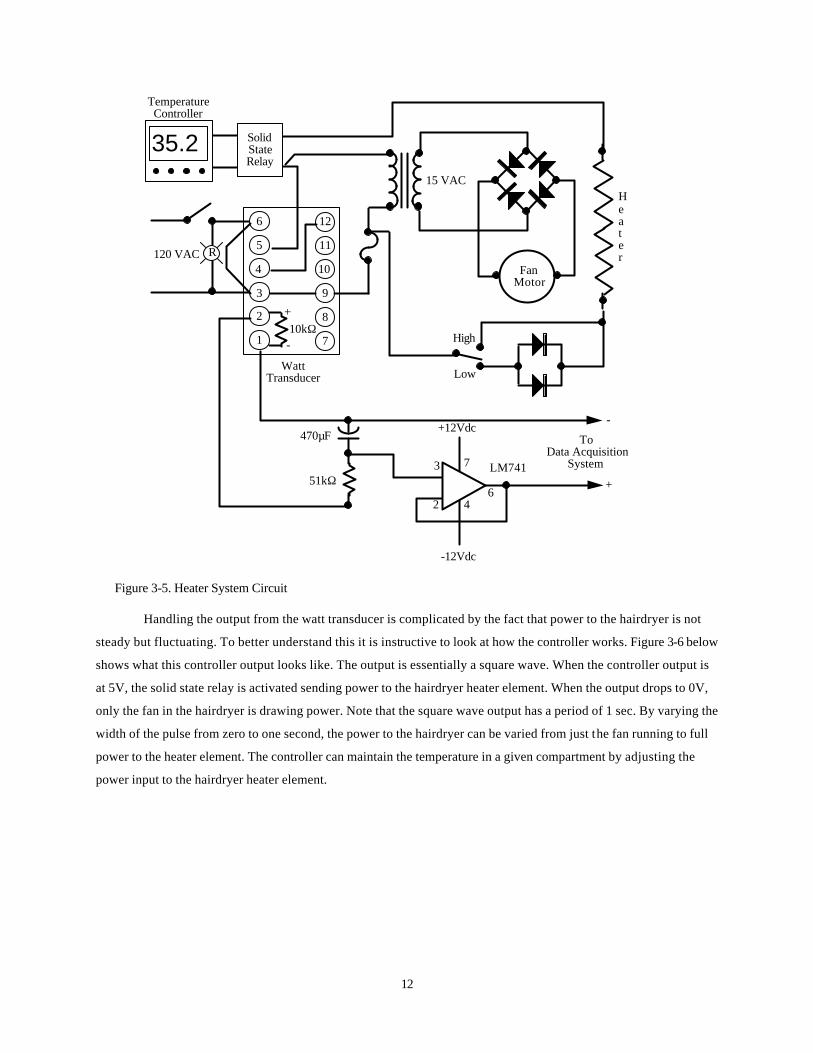
The electrical circuit for the heater system is shown in Figure 3-5. The control box contains the transformer

to drive the fan motor in the hairdryer and a solid state relay. It is the solid state relay that does the actual power

switching in response to the input signal from the PID controller. Since these components dissipate part of the

energy measured by the watt transducer, the control box is located inside the refrigerator as shown in Figure 3-4 to

eliminate a source of error in determining the load on the refrigerator.

The hairdryer is a standard commercially available model. The heater elements were wired in series to reduce

the maximum power output of the hairdryer. The high/low selector switch controls the power input to the heater

element, nominally either 300W or 150W respectively. Note that the fan is wired so that it runs continuously.

12

To Data Acquisition System3

2

+12Vdc

-12Vdc

4

7

6

LM741+

-

1

2

3

4

5

6

7

8

9

10

11

12

10kΩ+

-

51kΩ

470µF

Fan Motor

High

Low

15 VAC

R120 VAC

Watt Transducer

35.2

Temperature Controller

Solid State Relay

H e a t e r

Figure 3-5. Heater System Circuit

Handling the output from the watt transducer is complicated by the fact that power to the hairdryer is not

steady but fluctuating. To better understand this it is instructive to look at how the controller works. Figure 3-6 below

shows what this controller output looks like. The output is essentially a square wave. When the controller output is

at 5V, the solid state relay is activated sending power to the hairdryer heater element. When the output drops to 0V,

only the fan in the hairdryer is drawing power. Note that the square wave output has a period of 1 sec. By varying the

width of the pulse from zero to one second, the power to the hairdryer can be varied from just the fan running to full

power to the heater element. The controller can maintain the temperature in a given compartment by adjusting the

power input to the hairdryer heater element.

13

Controller Output

+5Vdc

0Vdc

320W

22W

sec.

sec.

sec.

1 2 3 4

Heater System Power

Conditioning Circuit Output

Figure 3-6. Heater System Control Signals

The heater system power in Figure 3-6 shows the theoretical response of the watt transducer to the

fluctuation in the power input to the hairdryer. It basically follows the square wave output of the controller. However,

the average power dissipated by the heater system is the quantity of interest not the instantaneous power. To obtain

the average power, a simple filter circuit containing a resistor and a capacitor was added to the output circuitry of the

watt transducer as shown in Figure 3-5. A time constant of 24 sec. was chosen for the RC network to reduce the

voltage ripple in the output to a minimum. The conditioning circuit output in Figure 3-6 shows a facsimile of the

result. This filtered signal is feed to the data acquisition system and converted into an average power measurement.

Finally the purpose of the operational amplifier should be noted. Measurements of the conditioned watt

transducer output with a voltmeter and the data acquisition system revealed a discrepancy. The data acquisition

system always measured a lower voltage. It was found that the input impedance of the data acquisition system is

only 200kΩ. Because the filter circuit contains resistances of the same order of magnitude as the input impedance of

the data acquisition system, the voltage signal is attenuated. To alleviate the problem, the operational amplifier was

added and wired to function as a voltage follower with essentially infinite input impedance and zero output

impedance. With the op-amp installed, no difference could be observed between the voltmeter and the data

acquisition system.

Because the complication of fluctuating power necessitated the need for filtering circuits, it is important to

verify that the actual power being utilized is correctly measured by the data acquisition system. It is also important to

determine if the watt transducer can respond to the fluctuating power signal without attenuation of the output. To

this end, Figure 3-7 shows a temporary modification to the heater system for the purpose of testing the accuracy of

the power measurements.

14

35.2 10kΩ

0-5kΩ

5kΩ

+12Vdc

10MΩ

+12Vdc

LN339 3kΩ4

5

3

212

Temperature Controller To

Solid State Relay

Oscilloscope

Figure 3-7. Power Verification Circuit

The circuit is the same as before except for the addition of a voltage comparator. Since the output of the

temperature controller is not a true square wave, it was difficult to determine exactly when the state, either on or off,

of the solid state relay changes. To remove this uncertainty, the voltage comparator shown was inserted between

the temperature controller and the solid state relay to clean up the output of the temperature controller. The

comparator was set with the potentiometer to trigger at 4.5 Vdc.

With a storage oscilloscope connected across the output of the comparator circuit, a direct measurement of

the amount of time the hairdryer heater element is drawing power during the one second cycle period can be made.

Further, the power utilized by the hairdryer when current is supplied continuously was measured with a voltmeter.

Two measurements of this kind were made, one with just the fan running and one with full power to the heater

element. These two power levels are constant. Given this fact, it is possible to calculate the average power dissipated

from

Average Power = (% heater on time)(full power) + (1-% heater on time)(fan power) (3.2)

where full power = 267W

fan power = 20W

Equation 3.2. The time percentages are calculated from the oscilloscope data. Note that this equation is only valid for

the one second cycle rate of the controller. Further note that the maximum and minimum power are dependent on line

voltage, which is not constant.

A comparison of the result from the calculation above can be made with a voltmeter measurement of the

output from the RC network of the watt transducer. If the watt transducer is correctly following the fluctuation in

power and the filter circuit is working properly, the two numbers should be the same. Table 3.1 shows the results of

the comparison. A maximum percent difference of -10.1% is reasonable. The watt transducers therefore are correctly

measuring the actual power being dissipated by the hairdryers.

15

Table 3.1. Watt Transducer Verification Data

Transducer Output (Vdc)

Watt Transducer Power

(W)

% Time at Full Power

Calculated Power

(W)

Error (%∆)

1.67 84 23 77 -8.3 1.62 81 25 81 0.0 1.68 84 28 89 6.0 2.75 138 42 124 -10.1 2.61 131 43 126 -3.8 2.56 128 43 126 -1.6 3.44 172 60 168 -2.3 3.3 165 60 168 1.8 3.29 165 60 168 1.8

Although the heater system works reasonably well some comments should be made about difficulties with

the system. The first difficulty concerns tuning the controllers. For reference, the settings for the controllers are listed

in Table 3.2. It was originally intended that both integral and proportional control would be used. However, it was

discovered that only the proportional function could be utilized. Using integral control resulted in oscillations in the

refrigerator compartment temperatures.

The cause is subtle. Even though the control signal may change state, a solid state relay has the

characteristic that it will not turn off or on until the line voltage passes through zero. It is not possible to turn the

relay off or on in the middle of a cycle. With a line frequency of 60Hz, power can only be delivered to the heaters in

discrete quantities of 1/120 of the total output from the heater i.e. one half cycle of power. As a result the output from

the heater does not vary continuously but changes in discrete steps. For the total heater output of 300W the power

changes in steps of 2W. Normally this small change would not be a problem. Unfortunately for a refrigerator though,

a few watts represents a measurable temperature change. Temperature oscillations occur because the controller

temperature resolution is smaller than the temperature change caused by 2W. To prevent the oscillations, the

solution is to turn off the integral control and only use proportional control. However, proportional control inherently

results in a temperature offset from the set point. Although this is not fatal it is a source of irritation because the

actual desired set point can not be inputed directly into the controller; the offset must be accounted for.

There are two improvements to the system that would be desirable. The first is replacing the pulse width

modulated output of the current controller with a proportional voltage output. This signal could be used to drive a

variac or the electronic equivalent of it. The variac would change the voltage level to vary the heater power instead of

the length of time full power is applied. A continuous current would eliminate the need for the RC circuit and make

performance verification easier. Further the elimination of the RC circuit would possibly allow some transient data to

be taken for which the current system is unsuitable. The second improvement would be to install a power

conditioning unit because the line voltage is not very stable. As a result, the maximum power output of the hairdryer

fluctuates making it harder on the controller system to maintain a constant temperature.

16

Table 3.2. Heater System Controller Settings

Freezer Controller Fresh Food Controller

Function # Setting Setting Function # Setting Setting

1 0.0 13 0 1 0.0 13 0 2 0.0 14 0 2 0.0 14 0 3 00 15 0 3 00 15 0 4 1 16 6 4 1 16 6 5 5 17 1 5 7 17 1 6 1 18 1 6 1 18 1 7 2 19 0 7 2 19 0 8 1 20 0 8 1 20 0 9 -1.8 21 0 9 -7.8 21 0

10 0 22 1 10 0 22 1 11 0 23 2 11 0 23 2 12 0 12 0

References [1] Reeves, R.N., Modeling and Experimental Parameter Estimation of a Refrigerator/Freezer System, Air

Conditioning and Refrigeration Center, Dept. of Mechanical and Industrial Engineering, University of Illinois at Urbana-Champaign, 1992, Chapter 5, pp. 30 to 41.

17

Chapter 4: Experimental Procedure

4.1 Refrigerator Testing For the purpose of parameter estimation, it is desirable to operate the refrigerator over the widest range of

test conditions as possible. To accomplish this both the evaporator inlet air temperature and the condenser inlet air

temperature must be varied. These two temperatures are the controlling parameters affecting the performance of the

vapor-compression system.

The condenser inlet air temperature was controlled by changing the operating temperature of the

environmental chamber. The refrigerator was run at four ambient temperatures: 55°F, 70°F, 90°F, and 100°F. At each

one of these ambient conditions the evaporator inlet air temperature was varied by changing the temperature settings

of the auxiliary heaters. The typical range of inlet temperatures was from 0°F to 70°F. For some test conditions it was

not possible to reach the upper temperature limit. This resulted from the fresh food compartment temperature

approaching the room ambient temperature with the heater in this compartment set at its' lowest power setting or

even off. At no time were either the fresh food compartment or the freezer compartment operated above ambient

conditions for the steady state tests. If this were to occur for a compartment, the cabinet heat load for that

compartment would be reversed.

For all tests the anti-sweat heater and the defrost controller were disabled. The defrost controller had to be

disconnected to prevent the refrigerator from going into a defrost cycle in the middle of a test. Further, the freezer

temperature control damper located in the fresh food compartment was set to the middle position. Lastly, the

refrigerator was positioned with the back of the refrigerator as close to the wall as possible without going below the

specified minimum clearance of one inch.

The refrigerant charge was optimized for steady-state operation by running a series of charge optimizing

tests. An explanation of the tests and the results can be found in Appendix C. The optimum charge was different for

the R12 and R134a tests. However, for each refrigerant tested the charge was kept constant for that refrigerant. The

system pressure when the refrigerator was turned off and the system temperatures equalized to 70°F was monitored.

If the pressure decreased by more than a few pounds, the system was recharged. Note that the pressure measured in

the system is below the saturation pressure at the ambient temperature of the system. It can't be directly concluded

that the refrigerant in the system is superheated. The presence of a large amount of oil, about 8 ounces, alters the

vapor pressure of the refrigerant. This effect must be considered when determining whether saturated or superheated

refrigerant exists in the system.

A typical test run involved inputting the desired temperatures for the fresh food comp artment and the

freezer compartment into the auxiliary heater system controllers. Usually it would take one to two hours for the

system to reach steady state. Some care should be exercised in deciding if the refrigerator has reached steady state.

For these tests, steady state conditions were assumed if after 50 minutes the average fresh food and freezer

compartment temperatures did not vary by more than 0.5°F during that time period. It was found that if shorter time

periods were taken such as 10 minutes it would appear that steady state conditions had been reached when in fact

the temperatures were still changing. Once steady state conditions had been reached data was collected every two

minutes for a minimum of at least one hour. This provided at least 30 measurements on which to base averages.

18

The refrigerator was operated as long as possible without having to allow the system to defrost. To facilitate

checking for frost, a small Plexiglass window was installed over a hole in the sheet metal divider between the

evaporator coil and the freezer compartment. Periodic checks were made to see how much frost had formed. When

noticeable frost formed on the coil, the system was shut down to allow the coil to warm up to melt the frost. The time

period between defrosts was usually two to three days.

Some comments should also be made about the heater system. As discussed in the instrumentation chapter,

the heat controllers had to be set up as proportional only controllers. A fundamental characteristic of proportional

control is the fact that there will always be an offset between the temperature entered into the controller and the

actual temperature in the system. This is somewhat inconvenient but the system will still provide the desired

temperature. The only complication is adding an offset to the temperature entered into the controller. Typically this

offset is of the order of 5°F to 10°F. Note that once steady state conditions have been reached a 2°F set point

change, for example, will result in a 2°F change in the measured temperature. Therefore the measured temperature can

be adjusted to the within the sensitivity limit of the controller or ±0.1°F.

The heater elements that are controlled are contained inside domestic hairdryers. The hairdryers were placed

in the bottom of each refrigerator compartment. Further, the hairdryers were positioned such that the warm air

discharge was directed toward the top of the compartment and away from the front of the refrigerator. In this way the

dynamic air pressure on the gaskets was minimized. It was found that the temperature gradient in the compartments

with the hairdryers operating was on the order of a few degrees. This is equivalent to the temperature gradients in the

compartments when the refrigerator is running in normal cycling operation. Lastly some care should be taken not to

run the hairdryers much above 105°F. At these elevated temperatures, the insulation on the motor windings break

down leading to the motor shorting out.

Some care should also taken to ensure that the operating pressures and temperatures don't exceed the range

over which the compressor is designed to operate. It is important that the discharge pressure does not go too far

above the highest recommended pressure. If the pressure is too high the discharge temperature will be high enough

to cause valve damage and accelerate the breakdown of the compressor oil. This will lead to compressor failure. The

suction side of the compressor should also be monitored. It is possible to have liquid refrigerant drawn into the

compressor even after going through the interchanger. This operating condition should be avoided because of the

potential of damage to the compressor.

Finally, the pressure transducers and the thermocouples were periodically checked for drift in calibration.

When the vapor compression system was open to the atmosphere for repairs or modifications, the gage pressure

transducers were zeroed. Further, the differential pressure transducers were zeroed when the system was turned off

and in equilibrium with the environment. The thermocouples that were accessible were immersed in an ice bath to

check their calibration. These procedures should be carried out particularly after modifications to the system or

instrumentation.

4.2 R134a Refrigerator Conversion The conversion of the refrigerator for use with R134a required four basic modifications to the vapor

compression system. The capillary tube/suction line interchanger had to be replaced. Further, the compressor was

19

replaced and the turbine flow meter was added. Lastly, the filter dryer had to be replaced with one that is compatible

with R134a.

After the old compressor and interchanger were removed, the system was flushed to eliminate as much of

the remaining mineral oil from the system as possible. Clean R11 was run from a refrigerant tank through the system

to another tank in ice water for a 24 hour period. The difference in vapor pressures forced the liquid R11 through the

system. The system was then evacuated for another day to remove any residual R11. The refrigerator was now ready

for the new components.

The capillary tube/suction line interchanger was replaced with the same size suction line and initially a

0.026" I.D. capillary tube as suggested [1]. The filter drier and the turbine flow meter were installed next. The new

compressor was installed last. The new compressor was charged with an ester oil. Since esters are hygroscopic, great

care was taken to make sure the compressor was exposed to the atmosphere for the shortest period of time as

possible.

Initial tests with the 0.026" capillary tube resulted in little cooling effect in the evaporator. As a result, the

capillary tube was replaced with the same size tube, 0.028" I.D., as was used in the original R12 system. For both cap

tube sizes, the length of the cap tube was progressively shortened and the effect on system performance determined.

The objective was to make the cap tube as short as possible thus increasing system capacity and still maintain

subcooling in the condenser. Subcooling in the condenser is an absolute necessity if the turbine flow meter is to

function properly. The final length of the cap tube for the R134a system was 10ft. It was noted that changes in cap

tube length have a small effect on system performance while changes in internal diameter have a large impact. Note

that after the R134a data set was taken the cap tube was shortened another two feet to see if lower superheat data

could be obtained. This modification did not change system performance at all.

Table 4.1 summarizes these modifications to the system. All other components were left unchanged from the

original R12 system.

Table 4.1. Summary of R134a System Modifications

Refrigerant Cap Tube Size

(I.D.) Cap Tube

Length (in.) Compressor

Model Compressor

Oil Displacement

Rate (ft3/hr)

R12 0.028" 80.7 MEI D123 Mineral Oil 53.2 R134a 0.028" 120 MEI D128 Ester - Kyoto

Oil # MR-5-22 67.2

References [1] Personal communication., Mr. Tom Benton., General Electric Company, Appliance Park, Louisville, Kentucky,

40225.

20

Chapter 5: Overview of Parameter Estimation

5.1 Refrigerator State Points Before looking at the models for the components in the refrigerator/freezer, it is helpful to touch on some of

the aspects of parameter estimation that is common to all the components. The first important topic is the

nomenclature for the state points used in the parameter estimation equations. Figure 5-1 shows the refrigeration

system in the refrigerator/freezer with the state points for each component labeled. The diagram also shows the

control volumes as dashed lines that were used for each component. The reader should refer to this diagram as

needed when reading Chapters 6 through 9.

Condenser

Suction Line Interchanger

Compressor

Door Heater

P10 T10

P1 T1

P3 T3

P4 T4

8"

Evaporator

P9 T9

P7 T7

Qevap.Qcomp.

Qcond.

Qdoor

P2 T2

P8 T8

Figure 5-1. Refrigerator/Freezer State Point Diagram

5.2 Optimization Techniques Two basic techniques were used to determine the best estimates of the parameters in the models. The first

method of non-linear least squares [1] was used for the interchanger and the compressor shell heat transfer

parameters. The method is relatively straight forward. Suppose for example that two quantities y and x are measured

in the lab. Further it is desired to find a functional relationship between y and x such that given an x value y can be

predicted. For the parameter estimation work considered here x is usually a temperature or pressure etc. and y is a

heat transfer rate. The functional relationship between the two variables must be assumed and usually comes from

such things as energy balances based on the first law of thermodynamics etc. For this discussion it is assumed that

this quantity y is related to the quantity x by Equation 5.1. Because of data scatter and the assumption that Equation

21

5.1 describes the physical process fully which may not be entirely true, the values of y predicted by Equation 5.1 for

a given x will not exactly equal the experimental y.

y = mx2 + b (5.1)

However, if the assumed functional relationship is good, the difference between the predicted y from

Equation 5.1 and the measured y will be small. It is natural to ask if it is possible to find values for the constants m

and b which will minimize this difference. Indeed, this minimum difference occurs when the derivative of Equation 5.1

with respect to the constants m and b for all the data points is zero. This statement is translated into mathematical

form by Equation 5.2 and 5.3 where n is the number of data points.

δδm

∑i=1

n

[ ]ymeasuredi - ypredictedi 2 = δ

δm ∑i=1

n

[ ]ymeasuredi - (mxi2 + b) 2 = 0.0 (5.2)

δδb

∑i=1

n

[ ]ymeasuredi - ypredictedi 2 = δδb

∑i=1

n

[ ]ymeasuredi - (mxi2 + b) 2 = 0.0 (5.3)

Equation 5.2 and 5.3 form a system of two equations in two unknowns, m and b. They can be solved for

example by a Newton-Raphson routine. Note that the differences are squared so that only positive errors are added.

For the parameter estimation work for the interchanger and the compressor, similar systems of non-linear equations

were solved by a commercial package called Engineering Equation Solver or E.E.S.[2].

This software has the great advantage of having refrigerant property routines are already built into the

program. This eliminates the need to develop separate property routines. The program also allows parametric studies

to be easily carried out. However, the program has an upper limit on the number of equations it can solve. As the

complexity of Equation 5.1, for example, increases the number of equations also increases. For the evaporator and the

condenser parameter estimation work, the number of equations exceeded the capability of the program. As a result a

different approach had to be taken.

This problem was solved by writing a computer program to find the best estimates of the parameters being

sought. The program was written in True Basic [3] and is listed in Appendix E. The general process of finding the

best estimates of the parameters involves calculating the sum of the squared differences between the measured and

predicted variables and deciding how to change the parameters to minimize these differences. The first major task

performed by the program is to calculate the sum of these differences for all data points or equivalently to evaluate

the objective function. A typical objective function for the condenser is given by Equation 5.4.

Objective Function = [ ]2n

1isubph2supdeii )U,U,U(crateQcQ∑ −

=

&& (5.4)

where Q. c = measured condenser heat transfer rate (Btu/hr)

Q. crate = predicted condenser heat transfer rate (Btu/hr)

n = number of data points

22

Udesup = conductance of desuperheating section (Btu/hr-ft2°F)

U2ph = conductance of two-phase section (Btu/hr-ft2°F)

Usub = conductance of the subcooled section (Btu/hr-ft2°F)

Q. cratei is determined from a system of effectivenes-NTU equations which contain the U parameters. These

equations will be discussed in Chapter 7. To solve this system of nonlinear equations, a set of Newton-Raphson

routines were used. The routines required are subroutine nr, subroutine calcfp, subroutine calcr, subroutine nzero

and subroutine xgauss (see Appendix E). The subroutine calcr contains the effectiveness-NTU relations in residual

form.

The subroutine object for objective function evaluates Equation 5.4 by calling the Newton-Raphson

routines for each data point and summing the squared error. Note that during the evaluation of Equation 5.4, the

parameters that are being sought; Udesup,U2ph, and Usub; are constants. Both the R12 and R134a data sets contain

approximately 30 points. One evaluation of the objective function requires the solution of approximately 30 sets of 12

simultaneous equations. This involves a fair amount of number crunching so an efficient optimization routine is a

necessity.

The next task is to vary the parameters Udesup,U2ph, and Usub such that the objective function is minimized. To

carry this out, the method of steepest-descent was used [4]. The basic process is to first calculate the gradient at the

current estimate of the parameters. The gradient indicates the direction of greatest change in the objective function.

The subroutine grad does the needed calculations. The next step is to search in the direction of the gradient to find a

new minimum in that direction. When this point is found the parameters are updated and the process is repeated.

The process continues until the components of the gradient vector approach zero which occurs at the true minimum

of the objective function.

The subroutine fibonacci (See Appendix E) performs the actual search procedure in the direction of the

gradient. The routine is based on a Fibonacci search method [4]. This method is more efficient than an exhaustive

search or dichotomous search because it requires the fewest number of function calls. As noted above each

objective function call is time consuming so it is very desirable to minimize the number of calls required. The routine

was written so that it could be used either to search for a minimum in a specified direction or perform a univariate

search in a direction parallel to a given parameter axis.

Unfortunately no one optimization method will work in all cases. Many types of problems can be

encountered. One problem that arises in this particular case is the existence of long, narrow, curved valleys in the

objective function. Contour plots for the actual surfaces will be shown in the appropriate chapters. Figure 5-2 shows

a contour plot of some hypothetical objective function. The method of steepest-descent will find a minimum for

example at a point formed by the intersection of lines aa and bb. However, once in the valley the method searches

back and forth across the valley, only very slowly progressing toward the true minimum.

To speed convergence it is necessary to search in a different direction. The direction to search in is found

by determining a new estimated minimum, i, near the old estimate. A linear curve fit of these two points forms a line,

indicated as the dotted line cc, directed along the valley floor. Searching along this line moves the estimated minimum

closer to the true minimum much mo re quickly. By repeating both the gradient search and this search routine, the true

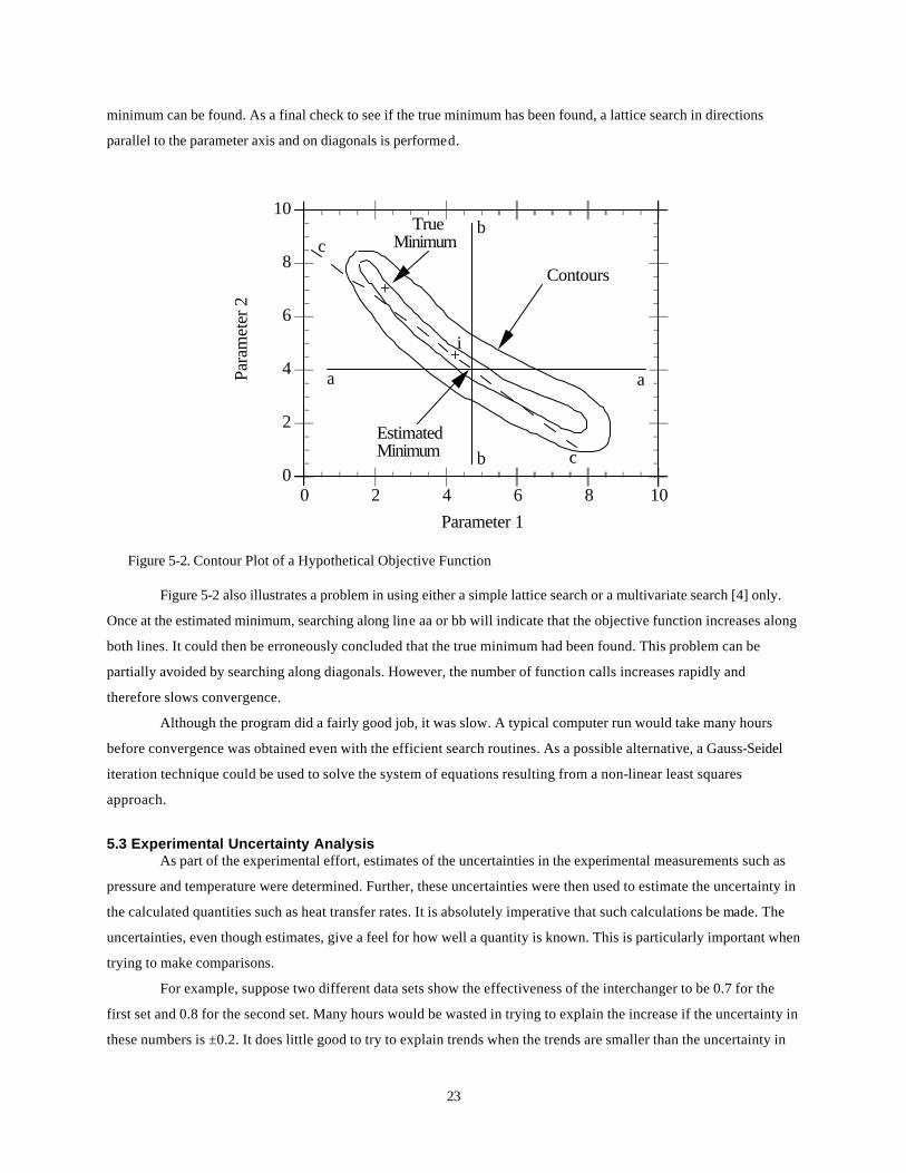
23

minimum can be found. As a final check to see if the true minimum has been found, a lattice search in directions

parallel to the parameter axis and on diagonals is performed.

0

2

4

6

8

10

0 2

Para

met

er 2

4 6 8 10Parameter 1

Contours

Estimated Minimum

True Minimum

a

+

+i

a

b

b c

c

Figure 5-2. Contour Plot of a Hypothetical Objective Function

Figure 5-2 also illustrates a problem in using either a simple lattice search or a multivariate search [4] only.

Once at the estimated minimum, searching along line aa or bb will indicate that the objective function increases along

both lines. It could then be erroneously concluded that the true minimum had been found. This problem can be

partially avoided by searching along diagonals. However, the number of function calls increases rapidly and

therefore slows convergence.

Although the program did a fairly good job, it was slow. A typical computer run would take many hours

before convergence was obtained even with the efficient search routines. As a possible alternative, a Gauss-Seidel

iteration technique could be used to solve the system of equations resulting from a non-linear least squares

approach.

5.3 Experimental Uncertainty Analysis As part of the experimental effort, estimates of the uncertainties in the experimental measurements such as

pressure and temperature were determined. Further, these uncertainties were then used to estimate the uncertainty in

the calculated quantities such as heat transfer rates. It is absolutely imperative that such calculations be made. The

uncertainties, even though estimates, give a feel for how well a quantity is known. This is particularly important when

trying to make comparisons.

For example, suppose two different data sets show the effectiveness of the interchanger to be 0.7 for the

first set and 0.8 for the second set. Many hours would be wasted in trying to explain the increase if the uncertainty in

these numbers is ±0.2. It does little good to try to explain trends when the trends are smaller than the uncertainty in

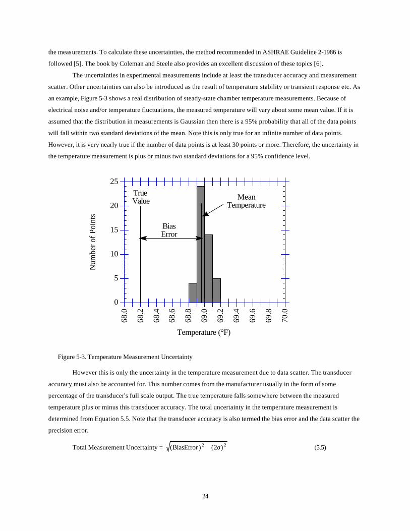
24

the measurements. To calculate these uncertainties, the method recommended in ASHRAE Guideline 2-1986 is

followed [5]. The book by Coleman and Steele also provides an excellent discussion of these topics [6].

The uncertainties in experimental measurements include at least the transducer accuracy and measurement

scatter. Other uncertainties can also be introduced as the result of temperature stability or transient response etc. As

an example, Figure 5-3 shows a real distribution of steady-state chamber temperature measurements. Because of

electrical noise and/or temperature fluctuations, the measured temperature will vary about some mean value. If it is

assumed that the distribution in measurements is Gaussian then there is a 95% probability that all of the data points

will fall within two standard deviations of the mean. Note this is only true for an infinite number of data points.

However, it is very nearly true if the number of data points is at least 30 points or more. Therefore, the uncertainty in

the temperature measurement is plus or minus two standard deviations for a 95% confidence level.

0

5

10

15

20

25

Num

ber o

f Poi

nts

68.0

68.2

68.4

68.6

68.8

69.0

69.2

69.4

69.6

69.8

70.0

Temperature (°F)

TrueValue

BiasError

MeanTemperature

Figure 5-3. Temperature Measurement Uncertainty

However this is only the uncertainty in the temperature measurement due to data scatter. The transducer

accuracy must also be accounted for. This number comes from the manufacturer usually in the form of some

percentage of the transducer's full scale output. The true temperature falls somewhere between the measured

temperature plus or minus this transducer accuracy. The total uncertainty in the temperature measurement is

determined from Equation 5.5. Note that the transducer accuracy is also termed the bias error and the data scatter the

precision error.

Total Measurement Uncertainty = 22 )2()BiasError( σ+ (5.5)

25

Once the total uncertainties in the measured quantities are known, the uncertainties in calculated quantities

can be determined. For example, the uncertainty in the heat transfer rate Q. in Equation 5.6 results from the

uncertainties in the mass flow rate m. and the enthalpies h2 and h1. The calculation of the uncertainty in Q

. is carried

out by evaluating Equations 5.7 and 5.8 for both enthalpies where w() is understood to mean the uncertainty of the

quantity within the brackets.

)1h2h(mQ −= && (5.6)

222

)2h(w2h

Q)1h(w1h

Q)m(wmQ)Q(w

δδ+

δδ+

δδ=

&&&

&

&& (5.7)

where

22

)P(wPh

)T(wTh

)h(w

δδ

+

δδ

= (5.8)

Each term in brackets is the uncertainty of a given independent variable multiplied by the sensitivity of

Equation 5.6 to that independent variable. The derivatives can be evaluated mathematically or numerically. In either

case, nominal values of the independent variables must be substituted into the derivative expressions to determine

the sensitivities. It is possible that the uncertainty of an independent variable is high while the sensitivity is very

small making the uncertainty of the dependent variable with respect to this independent variable small. The converse

can also occur.

The terms in brackets in Equations 5.7 and 5.8 also have another useful purpose. Instead of asking how

uncertain is the heat transfer rate given the data reduction equation and instrumentation, the reverse question can be

asked. How certain do the experimental measurements have to be so that the heat transfer rate is known to within a

specified accuracy? This question can be answered by looking at the magnitude of each term inside the brackets of

Equation 5.7. For example, it is desired to know the heat transfer rate to within ±50 Btu/hr. The first term in brackets in

Equation 5.7 might equal 80 Btu/hr. It could then be concluded that either the accuracy of the mass flow measurement

must be increased or some alternate equation that is not as sensitive to mass flow rate must be found. The same

analysis can be carried out for each term. However, since each uncertainty is squared, the terms inside the brackets

that are larger in magnitude will tend to dominate the uncertainty in the heat transfer rate. Therefore, improvements

should be concentrated on these terms first.

This analysis should be carried out before ever going into the lab and taking measurements. It is a total

waste of time to spend months setting up instrumentation and taking data only to find out later that the accuracy of a

given transducer did not allow determining a quantity to within the desired accuracy. The instrumentation and the

equations that are going to be used must be investigated first. Changes in instrumentation or experimental methods

up front will help to ensure that the desired results are obtained later.

Equation 5.7 only determines the uncertainty in the heat transfer rate as a result of the experimental

uncertainties. For some of the parameter estimation work, a parameter is estimated which is theoretically a constant

26

such as volumetric flow rate. As a result of scatter in the data, the estimated parameter will be a mean value. A total

uncertainty calculated from Equation 5.5 is needed to reflect both the experimental uncertainty and the scatter in the

estimates. The standard deviation is based on the differences between the average estimated flow rate and that

calculated for each data point.

The calculation of the experimental uncertainties of the measured quantities and calculated parameters are

listed in Appendix D. Unless otherwise noted, a given uncertainty is the experimental uncertainty in a parameter, not

the total uncertainty. The total uncertainty, where given, will be labeled explicitly. The reader should refer to the

calculations in Appendix D as needed to see where the uncertainties originate.

References [1] Stoecker, W.F., Design of Thermal Systems , Third Edition, McGraw-Hill, New York, 1989, pp. 67 to 70.

[2] E.E.S., F-Chart Software, 4406 Fox Bluff Road, Middleton, WI, 53562.

[3] True Basic., True Basic, Inc., 39 South Main St., Hanover, N.H., 03755.

[4] Stoecker, W.F., Chapter 9.

[5] Engineering Analysis of Experimental Data - ASHRAE Guideline 2-1986., (Available from American Society of Heating, Refrigerating and Air-Conditioning Engineers, Inc., 1791 Tullie Circle, N.E., Atlanta, GA 30329.

[6] Coleman, H.W. and W.G. Steele., Experimentation and Uncertainty Analysis for Engineers, John Wiley & Sons, New York, 1989.

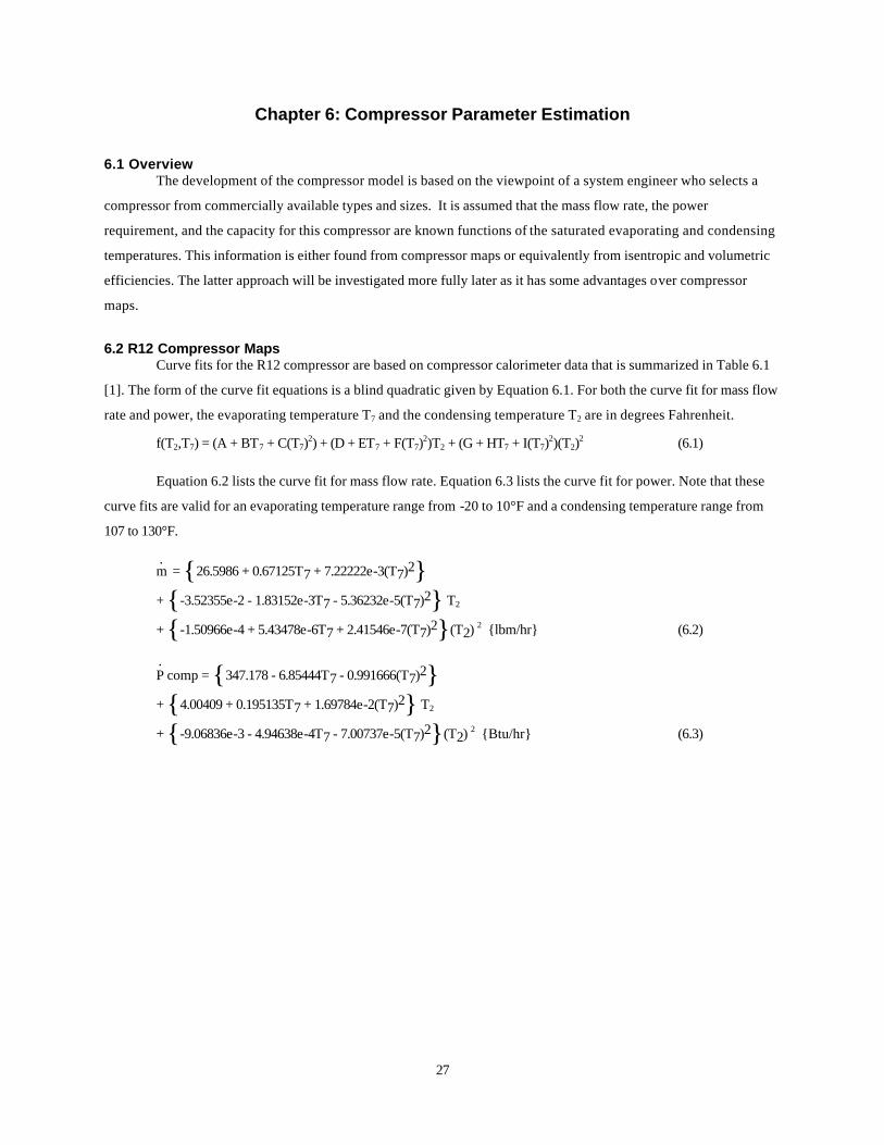
27

Chapter 6: Compressor Parameter Estimation

6.1 Overview The development of the compressor model is based on the viewpoint of a system engineer who selects a

compressor from commercially available types and sizes. It is assumed that the mass flow rate, the power

requirement, and the capacity for this compressor are known functions of the saturated evaporating and condensing

temperatures. This information is either found from compressor maps or equivalently from isentropic and volumetric

efficiencies. The latter approach will be investigated more fully later as it has some advantages over compressor

maps.

6.2 R12 Compressor Maps Curve fits for the R12 compressor are based on compressor calorimeter data that is summarized in Table 6.1

[1]. The form of the curve fit equations is a blind quadratic given by Equation 6.1. For both the curve fit for mass flow

rate and power, the evaporating temperature T7 and the condensing temperature T2 are in degrees Fahrenheit.

f(T2,T7) = (A + BT7 + C(T7)2) + (D + ET7 + F(T7)

2)T2 + (G + HT7 + I(T7)2)(T2)

2 (6.1)

Equation 6.2 lists the curve fit for mass flow rate. Equation 6.3 lists the curve fit for power. Note that these

curve fits are valid for an evaporating temperature range from -20 to 10°F and a condensing temperature range from

107 to 130°F.

m. = 26.5986 + 0.67125T7 + 7.22222e-3(T7)2

+ -3.52355e-2 - 1.83152e-3T7 - 5.36232e-5(T7)2 T2

+ -1.50966e-4 + 5.43478e-6T7 + 2.41546e-7(T7)2 (T2) 2 lbm/hr (6.2)

P. comp = 347.178 - 6.85444T7 - 0.991666(T7)2

+ 4.00409 + 0.195135T7 + 1.69784e-2(T7)2 T2

+ -9.06836e-3 - 4.94638e-4T7 - 7.00737e-5(T7)2 (T2) 2 Btu/hr (6.3)

28

Table 6.1. R12 Compressor Calorimeter Data

T2 °F

T7 °F

Capacity Btu/hr

Power W

Discharge Temperature °F

Suction Temperature °F

Flow Rate lbm/hr

-20 107 746 149 199 92 12 -20 107 752 152 200 94 12.1 -10 107 997 172 203 91 16.1 -10 107 1006 174 204 94 16.2 10 107 1659 221 206 91 26.9 10 107 1654 223 207 92 26.9 -20 115 718 152 201 92 11.6 -20 115 724 153 202 95 11.6 -10 115 965 175 206 91 15.6 -10 115 971 177 207 94 15.7 10 115 1618 228 210 90 26.3 10 115 1620 230 211 92 26.3 -20 130 666 153 207 93 10.7 -20 130 667 154 206 95 10.7 -10 130 908 180 212 92 14.6 -10 130 909 181 212 94 14.7 10 130 1543 240 222 92 25.1 10 130 1549 240 221 93 25.2

Figure 6-1 compares the predicted mass flow rate from Equation 6.2 to the calorimeter data from Table 6.1. As

can be seen the biquadratic curve fit does a good job at matching the calorimeter data. The error bounds are ±0.4%

with a standard deviation of 0.17%. The total uncertainty in the mass flow rate prediction is unknown because the

experimental error in the measurements in Table 6.1 are unknown. However, typical total uncertainties in compressor

maps are of the order of ±5% [2,3]. Figure 6-2 compares the predicted compressor power input from Equation 6.3 to

the calorimeter data. As for the mass flow rate, the curve fit does a nice job at matching the calorimeter data. The

maximum curve fit error is ±1.0% with a standard deviation of 0.26%.

Although compressor maps do a fairly good job at predicting compressor performance, there are several

problems associated with their use. The first problem relates to the calorimeter data. As can be seen from Table 6.1,

the suction gas temperature at the compressor inlet is kept nearly constant at 90°F. For the refrigerator tested at the

standard rating condition of 90°F the suction temperature is indeed close to 90°F. However, the experimental data for

the refrigerator using R12 showed the suction temperature to vary from 47°F to 102°F. The variation in suction

temperature causes the suction specific volume to change which affects compressor performance. To account for the

variation in suction temperatures, it is necessary to apply a correction factor to the map data. For a discussion of the

effect of superheat on compressor performance and possible correction factors see Dabiri and Rice [4].

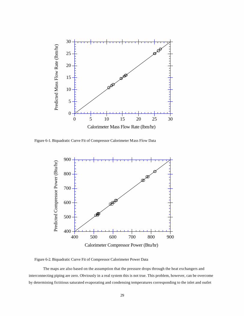
29

0

5

10

15

20

Pred

icte

d M

ass

Flow

Rat

e (lb

m/h

r)25

30

0 5 10

Calorimeter Mass Flow Rate (lbm/hr)

15 20 25 30

Figure 6-1. Biquadratic Curve Fit of Compressor Calorimeter Mass Flow Data

400

500

600

700

800

900

400 500

Pred

icte

d C

ompr

esso

r Pow

er (B

tu/h

r)

600 700 800 900

Calorimeter Compressor Power (Btu/hr)

Figure 6-2. Biquadratic Curve Fit of Compressor Calorimeter Power Data

The maps are also based on the assumption that the pressure drops through the heat exchangers and

interconnecting piping are zero. Obviously in a real system this is not true. This problem, however, can be overcome

by determining fictitious saturated evaporating and condensing temperatures corresponding to the inlet and outlet

30

pressures to the compressor. Using these temperatures in Equations 6.2 and 6.3 results in a better estimate of the

mass flow rate and power consumption in the actual system.

A more difficult problem from an experimental perspective is the limited range of the maps. Figure 6-3 shows

all the R12 data points plotted as a function of evaporating and condensing temperatures. The box indicates the

range in which the compressor maps are applicable. As can be seen from the graph, only half of the data fall within

the range for which the maps can be utilized.

70

80

90

100

110

120

130

Con

dens

ing

Tem

pera

ture

(°F)

140

-25 -20 -15 -10 -5 0Evaporating Temperature (°F)

5 10 15

Map Envelope

Figure 6-3. Comparison of R12 Data Set to Compressor Map Range

6.3 Volumetric Efficiency Approach for the R12 Compressor For the purpose of parameter estimation is would be very desirable to use the entire data set. To make this

possible, an alternative to the compressor maps must be found. The method finally used takes advantage of the

performance characteristics of a reciprocating compressor. For a reciprocating compressor, the mass flow rate

through the compressor is given by Equation 6.4 [5].

suc

dispv

Vm

υη=& (6.4)

where m? = mass flow rate (lbm/hr)

ηv = volumetric efficiency

Vdisp = displacement rate (ft3/hr)

υsuc = suction specific volume (ft3/lbm)

31

Further, the power consumed by the compressor can be described by Equation 6.5.

s

sPP

η=

&& (6.5)

where P. = compressor power consumption (W or Btu/hr)

P. s = isentropic power consumption (W or Btu/hr)

ηs = isentropic efficiency

By utilizing the calorimeter data in Table 6.1, both the volumetric efficiency and is entropic efficiency can be

determined. The volumetric efficiency can be calculated from the mass flow rate, inlet conditions, and the

displacement rate. The displacement rate of a reciprocating compressor is a physical characteristic of the compressor

and is assumed to be a constant. For the compressor used in the R12 experiments, the displacement rate is 53.188

ft3/hr [6]. Fortunately, the volumetric efficiency is very nearly a linear function of the absolute pressure ratio of the

condensing pressure to the evaporating pressure only [7]. The volumetric efficiency for this compressor as a

function of pressure ratio is shown in Figure 6-4.

The value of this approach over using compressor maps lies in the fact that the pressure ratios for all the

R12 data points are within the upper and lower bounds of Figure 6-4. Stated differently: for the R12 data points

having condensing or evaporating pressures outside the map bounds, it turns out that the ratio of those pressures

are within the bounds of the range of ratios in Figure 6-4. The range of the compressor maps can, therefore, be

effectively extended by using a volumetric efficiency approach.

0.00

0.20

0.40

0.60

0.80

1.00

Vol

umet

ric E

ffic

ienc

y

0 5 10 15

ηv = 0.926478 - 0.02298(Pc/Pe)

Absolute Pressure Ratio (Pc/Pe)

Figure 6-4. Volumetric Efficiency Curve for the R12 Compressor

32

The use of volumetric efficiency instead of maps also eliminates the problem with varying suction

temperatures. Because Equation 6.4 is a function of the suction specific volume, any changes in suction temperature

will be reflected in this parameter. The suction specific volume, therefore, automatically accounts for variations in

suction temperature. The problem of pressure loss in the heat exchangers is also avoided because Equation 6.4 only

depends on inlet and outlet conditions to the compressor.

A similar approach can be used for the compressor power. Like the volumetric efficiency, the isentropic

efficiency was determined from the compressor calorimeter data. Further, the isentropic efficiency is also very nearly

a linear function of the absolute pressure ratio only. The isentropic power is easily calculated from the compressor

inlet pressure and temperature, and outlet pressure. Figure 6-5 shows the relationship between isentropic efficiency

and the absolute pressure ratio across the compressor. As with the volumetric efficiency, using an isentropic

efficiency effectively extends the range of applicability of the compressor maps.

To check the accuracy of the above approach, it is instructive to compare the mass flow rates and powers

determined from Equations 6.4 and 6.5 against the measured values in Table 6.1. Figure 6-6 compares the calculated

flow rates against the calorimeter data. As can be seen, the agreement between the calculated mass flow rates and the

calorimeter values is very good. The maximum deviation of the predicated flow rates from the calorimeter mass flow

rates is ±1.5% with a standard deviation of 0.38%. The same comparison can be made for the compressor power.

0.00

0.20

0.40

0.60

0.80

1.00

0 5 10

Isen

tropi

c Ef

ficie

ncy

15

ηs = 0.5518 - 0.00214(Pc/Pe)

Absolute Pressure Ratio (Pc/Pe)

Figure 6-5. Isentropic Compressor Efficiency Curve for the R12 Compressor

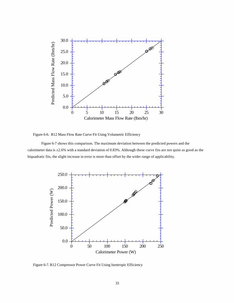
33

0.0

5.0

10.0

15.0

20.0

Pred

icte

d M

ass

Flow

Rat

e (l

bm/h

r)25.0

30.0

0 5 10Calorimeter Mass Flow Rate (lbm/hr)

15 20 25 30

Figure 6-6. R12 Mass Flow Rate Curve Fit Using Volumetric Efficiency

Figure 6-7 shows this comparison. The maximum deviation between the predicted powers and the

calorimeter data is ±2.6% with a standard deviation of 0.83%. Although these curve fits are not quite as good as the

biquadratic fits, the slight increase in error is more than offset by the wider range of applicability.

0.0

50.0

100.0

150.0

200.0

250.0

0

Pred

icte

d Po

wer

(W)

50 100 150 200 250Calorimeter Power (W)

Figure 6-7. R12 Compressor Power Curve Fit Using Isentropic Efficiency

34

6.4 Volumetric Efficiency Curve Fits for the R134a Compressor Converting the refrigerator for use with R134a required replacing the R12 compressor with a compressor

having a larger volumetric displacement. Compressor maps were not available for the new compressor using R134a.

To take their place, the mass flow rate through the system was measured with a turbine flow meter. Further, the power

input was also measured directly. These measurements provided all the necessary information for parameter

estimation. However, for the purpose of modeling the new compressor, the volumetric efficiency and isentropic

efficiency are needed.

The volumetric efficiency from Equation 6.4 was calculated for all points in the R134a data set and plotted

against the absolute pressure ratio in Figure 6-8. The experimental uncertainty in the volumetric efficiency is ±0.056

with a standard deviation in the linear curve fit of 0.03. The total uncertainty in the equation for volumetric efficiency

is ±0.082. The volumetric efficiencies are based on the compressor having a displacement rate of 67.2 ft3/hr [8]. Note

that the large uncertainty in the absolute pressure ratio is caused by the uncertainty in the suction pressure (see

Appendix D).

The y-intercept for the volumetric efficiency equation is 1.27 which is physically not possible. This suggests

that the volumetric efficiency is not a linear function of absolute pressure ratio from a pressure ratio of 0 to 16. The

equation should, therefore, only be used within the upper and lower bounds of the pressure ratios shown.

0.0

0.2

0.4

0.6

0.8

1.0

Vol

umet

ric E

ffic

ienc

y

10 11 12 13 14 15Absolute Pressure Ratio (Pc/Pe)

16

ηv = 1.2757 - 0.043077(Pc/Pe)

Figure 6-8. Volumetric Efficiency for R134a Compressor

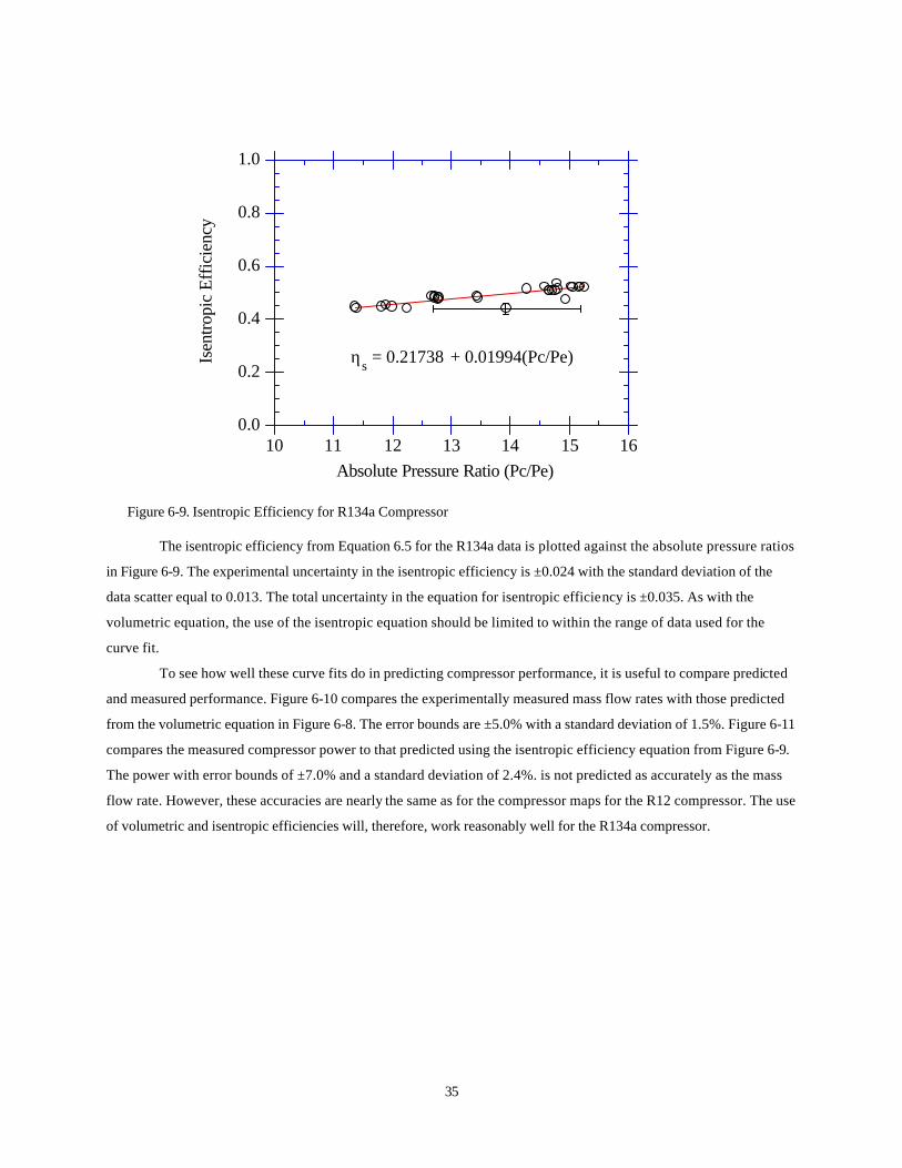
35

0.0

0.2

0.4

0.6

0.8

1.0

10

Isen

tropi

c Ef

ficie

ncy

11 12 13 14 15 16Absolute Pressure Ratio (Pc/Pe)

ηs = 0.21738 + 0.01994(Pc/Pe)

Figure 6-9. Isentropic Efficiency for R134a Compressor

The isentropic efficiency from Equation 6.5 for the R134a data is plotted against the absolute pressure ratios

in Figure 6-9. The experimental uncertainty in the isentropic efficiency is ±0.024 with the standard deviation of the

data scatter equal to 0.013. The total uncertainty in the equation for isentropic efficiency is ±0.035. As with the

volumetric equation, the use of the isentropic equation should be limited to within the range of data used for the

curve fit.

To see how well these curve fits do in predicting compressor performance, it is useful to compare predicted

and measured performance. Figure 6-10 compares the experimentally measured mass flow rates with those predicted

from the volumetric equation in Figure 6-8. The error bounds are ±5.0% with a standard deviation of 1.5%. Figure 6-11

compares the measured compressor power to that predicted using the isentropic efficiency equation from Figure 6-9.

The power with error bounds of ±7.0% and a standard deviation of 2.4%. is not predicted as accurately as the mass

flow rate. However, these accuracies are nearly the same as for the compressor maps for the R12 compressor. The use

of volumetric and isentropic efficiencies will, therefore, work reasonably well for the R134a compressor.

36

5

6

7

8

9

10

5.0 6.0 7.0

Pred

icte

d M

ass

Flow

Rat

e (lb

m/h

r)

8.0 9.0 10.0

±5.0%

Measured Mass Flow Rate (lbm/hr)

Figure 6-10. R134a Mass Flow Rate Curve Fit Using Volumetric Efficiency

110

120

130

140

150

160

170

Pred

icte

d C

ompr

esso

r Pow

er (W

)

110 120 130 140 150 160 170

±7.0%

Measured Compressor Power (W)

Figure 6-11. R134a Compressor Power Curve Fit Using Isentropic Efficiency

37

6.5 Compressor Shell Heat Transfer Compressor maps or equivalently volumetric and isentropic efficiencies don't entirely characterize the

performance of a compressor. It is also necessary to know the amount of heat transfer from the compressor shell. For

the compressors studied this heat transfer is not negligible.

The simplest model to correlate heat transfer from the compressor shell with compressor operating

conditions is to assume a constant convective film coefficient over the entire compressor shell. With this film

coefficient known, the heat transfer rate from the compressor shell can be calculated from Equation 6.6. The

temperature difference chosen to base the film coefficient on is

Q. comp = h

_ ∆T (6.6)

somewhat arbitrary. Since the compressor shells for the units tested were on the discharge side of the compressor,

the discharge temperature minus the ambient temperature was taken as the most appropriate temperature difference.

To determine the best film coefficients for both the R12 and R134a compressors, a non-linear least squares

worksheet in E.E.S. was formulated (See Appendix E for listing). The equations to be solved are given in Equations

6.7 through 6.10. Equation 6.7 determines the compressor heat transfer from the measured power requirement,

refrigerant mass flow rate and inlet and outlet conditions to the compressor. Equation 6.8 calculates the condenser

fan power requirement. This quantity is not measured directly. Equation 6.9 determines the temperature of the air

surrounding the compressor shell, Tcompairi, from an air-side energy balance across the condenser fan. Once these

quantities are calculated for all the data points, Equation 6.10 can be evaluated to determine the best estimate of h _

.

Q. comp i = (3.413 P

. comp i ) - m

. i (h1i - h10i ) i = 1,n (6.7)

P. confani = P

. systemi - P

. comp i - P

. evapfani i = 1,n (6.8)

3.413 P. confani = 60ρCpV

. (Tconfanouti - Tcompairi) i = 1,n (6.9)

[ ] 0.0n

1i)iTcompairi1T(hicompQ

h

2

==

−−δδ ∑ & (6.10)

where Q. comp = compressor shell heat transfer (Btu/hr)

P. comp = compressor power input (W)

m. = refrigerant mass flow rate (lbm/hr)

h1 = enthalpy at the compressor discharge (Btu/lbm)

h10 = enthalpy at the compressor inlet (Btu/lbm)

P. confan = condenser fan power (W)

P. system = total refrigerator power (W)

38

P. evapfan = evaporator fan power (W)

Tconfanout = condenser fan outlet air temperature (°F)

Tcompair = air temperature surrounding compressor (°F)

T1 = compressor discharge temperature (°F)

Solving Equation 6.10 for the R12 data set results in a convective film coefficient of 5.92 Btu/hr°F ±0.2

Btu/hr°F. The slope of the line in Figure 6-12 is equal to the film coefficient. Note also that the exp erimental

uncertainty is the same order of magnitude as the scatter in the data. This suggests that some of the model

assumptions are incorrect. One very likely source of error is assuming that the surface temperature of the compressor

shell is uniform. However, even with this assumption, the heat transfer from the R12 compressor shell as shown in

Figure 6-13 can be predicted to within ±8.0% with a standard deviation of 1.9%. It is doubtful that this model can be

improved without making it a great deal more complicated.

Repeating the same calculations for the R134a data set results in a convective film coefficient of 5.83

Btu/hr°F ±0.2 Btu/hr°F. Within the experimental uncertainty this is the same as the film coefficient for the R12

compressor. This is a logical result because both compressors have very similar shell geometries and the same airflow

rates over the shell. However, it is unlikely that this film coefficient will work for other geometries. The slope of the

line in Figure 6-14 is the film coefficient for the R134a compressor. As for the R12 case, the scatter in the data is the

same order of magnitude as the experimental uncertainty. Figure 6-15 shows that the constant film coefficient model

does a somewhat worse job for the R134a data with error bounds of ±10% and a standard deviation of 2.1%.

However, this is still a reasonable amount of error.

0

100

200

300

400

500

Shel

l Hea

t Tra

nsfe

r (B

tu/h

r)

600

0 20 40 60 80 100T1-Tcompair (°F)

Figure 6-12. Convective Film Coefficient for the R12 Compressor

39

300

350

400

450

500

550Pr

edic

ted

Com

pres

sor S

hell

Hea

t Tra

nsfe

r(B

tu/h

r)

600

300 350 400 450 500Experimental Compressor Shell Heat Transfer

(Btu/hr)

550 600

±8.0%

Figure 6-13. R12 Compressor Shell Heat Transfer

0

100

200

300

400

500

Shel

l Hea

t Tra

nsfe

r (B

tu/h

r)

0 10 20 30 40 50 60

T1-Tcompair (°F)

70 80

Figure 6-14. Convective Film Coefficient for R134a Compressor

40

300

340

380

420

460

500

300

Pred

icte

d C

ompr

esso

r She

ll H

eat T

rans

fer

(Btu

/hr)

340 380 420 460 500

±10%

Experimental Compressor Shell Heat Transfer(Btu/hr)

Figure 6-15. R134a Compressor Shell Heat Transfer

6.6 Conclusions The constant convective film coefficient model does a reasonably good job. The model was able to predict

heat transfer from the compressor shell to with ±8.0% for the R12 compressor and ±10.0% for the R134a compressor.

Improvements in the model will probably require a large increase in complexity such as making the compressor shell

surface temperature a function of location on the compressor. It is questionable whether the added complexity is

justified.

These results are restricted to small reciprocating compressors that have the compressor shell on the

discharge side of the compressor. Other compressor types such as rotary compressors should be investigated.

Further, compressors where the compressor shell is on the low side of the compressor should also be looked at.

For the purpose of modeling the other compressor performance parameters such as mass flow rate etc., the

use of either compressor maps or volumetric efficiencies work equally well. However, the volumetric efficiency

approach has the advantage of not requiring any correction factors for superheat. The volumetric efficiency

approach also has the advantage of being applicable to a wider range of conditions. This can be an advantage in

analyzing experimental data.

References [1] Personal communication., Mr. Spike Kline., General Electric Company, Appliance Park, Louisville, Kentucky,

40225.

[2] Reeves, R.N., Modeling and Experimental Parameter Estimation of a Refrigerator/Freezer System, Air Conditioning and Refrigeration Center, Dept. of Mechanical and Industrial Engineering, University of Illinois at Urbana-Champaign, 1992, p. 66.

41

[3] Copeland Copeleweld Data Book, Copeland Corporation, Sidney, Ohio (1990).

[4] Dabiri, A.E. and C.K. Rice. 1981. "A Compressor Simulation Model with Corrections for the Level of Suction Gas Superheat.", ASHRAE Transactions,Vol. 87, Part 2, pp. 77 to 782.

[5] Stoecker, W.F. and J.W. Jones, Refrigeration and Air Conditioning, McGraw-Hill, New York, 1986, Chapter 11.

[6] Personal communication , Mr. John Driver, General Electric Company, Appliance Park, Louisville, Kentucky, 40225.

[7] Stoecker, p. 217.

[8] Personal communication., Mr. Spike Kline., General Electric Company, Appliance Park, Louisville, Kentucky, 40225.

42

Chapter 7: Condenser Parameter Estimation

7.1 Overview The condenser model is based in part on the work by Reeves [1] and Kempiak and Crawford [2]. Kempiak

and Crawford modeled a condenser in a mobile air-conditioning system. Their model considers the condenser to be a

long tube within which there are three zones that have different heat transfer characteristics. The zones are: a

desuperheating section in which refrigerant vapor transfers heat with air, a two-phase section in which saturated

refrigerant transfers heat with air, and a subcooled section in which heat exchange is between liquid refrigerant and

air. For each section an overall heat transfer coefficient or UA value and fraction of that section's length to the total

was determined. The UA value was considered a function of condenser air flow rate and refrigerant mass flow rate.

The model was able to predict the total heat transfer from the condenser to within ±1.8%.

Reeves adapted this approach to domestic refrigerator/freezer condensers. The model was somewhat

simplified because variations in condenser air flow rate were not considered. Further, rather than determine a fraction

of a given section length to the total, equivalently an appropriate surface area proportional to the section length was

determined. With this area known, the UA for a given section (x) can be split into a conductance U based on surface

area A. To accomplish this, it is necessary to make some assumptions. Equation 7.1 relates the overall heat transfer

coefficient for a given section to the thermal resistances inside and outside of the tube and of the tube itself [3].

ii

io

oo Ah1

Lk2)r/rln(

Ah1

UxAx1

+π

+= (7.1)

where Ux = overall conductance based on A x

Ax = arbitrary surface area

ho = air side convective film coefficient

Ao = effective air side surface area

ro = outside radius of condenser tube

ri = inside radius of condenser tube

L = length of a given condenser section

k = thermal conductivity of tube

hi = refrigerant side convective film coefficient

Ai = effective refrigerant side surface area

Since the air flow rate across the condenser is not varied, the convective film coefficient on the outside can

be assumed to be constant if variations in thermodynamic properties are considered negligible. Likewise, the

resistance of the wall is also constant. The refrigerant film coefficient is a function of mass flow rate. If the mass flow

rate does not vary significantly, then the internal coefficient can also be assumed constant. With these assumptions

Equation 7.1 can be rewritten as Equation 7.2. Solving Equation 7.2 for Ux yields Equation 7.3. The result is if the film

coefficients are assumed to be constants then the conductance for that section is also constant. This is the basis for

assuming that the conductances for each section of the condenser are constant.

43

LK

L1

DCh1

k2)r/rln(

DCh1

LDCU1 1

i3i

io

o2ox1x=

π

+π

+π

=π

(7.2)

where C1,C2,C3 and K1 = constants

Dx = diameter associated with surface area Ax

Do = outside diameter of condenser tube

Di = inside diameter of condenser tube

Ux = 1

K1C1πDx = constant (7.3)

The same constant U model can also be derived from the assumption that the air side resistance dominates

the heat transfer process in the condenser. If this is true then the tube wall and refrigerant side resistances can be

neglected. Further, since the air side volumetric flow rate is constant, the resistance or conversely the conductance

will be constant if changes in thermodynamic properties are small. A necessary consequence of the air side

resistance dominating the heat transfer process is the fact that the U values for all sections will be the same; the

effect of the refrigerant side being negligible. Indeed, Reeves found that the desuperheating and the two-phase

sections had nearly the same conductance. However, in the subcooled section the U value was half that of the

desuperheating and two-phase sections. This indicates that the internal resistance of the liquid refrigerant does have

an impact on the overall heat transfer coefficient. This suggests that the U for this section is a function of refrigerant

mass flow rate and therefore not constant.

A possible improvement to a constant U assumption is to make the U's for each section of the condenser a

function of refrigerant mass flow rate. Equation 7.1 could then be written in the form of Equation 7.4. The constant B1

includes the constant air side resistance and wall resistance The constant B2 is a ratio of areas.

hi2B

BU1

1x

+= (7.4)

where B1,B2 = constants

The constant U approach and a refrigerant mass flow dependent U method will be considered for both the

R12 and R134a cases. Like Reeves, effectiveness - NTU relations in conjunction with estimated conductances will be

used to predict condenser performance. However, before the U parameters can be estimated from the experimental

data, it is necessary to determine the condenser volumetric air flow rate. This quantity must be known in order to

evaluate the effectiveness-NTU relations.

7.2 Condenser Volumetric Flow Rate The volumetric air flow rate was determined by equating a refrigerant side and air side energy balance. The

most obvious choice is to set the condenser heat rejection equal to the air temperature rise across the coil. However,

the air temperature at the exit of the condenser was too difficult to accurately measure. A much more suitable location

to measure an air temperature is downstream of the condenser fan. The temperature difference between this point and

the condenser inlet is the result of heat transfer from not only the condenser but also from the compressor and the

condenser fan.

44

Figure 7-1 shows the layout of the underside of the refrigerator as viewed from above. The condenser air

inlet is at the front of the refrigerator. The condenser is a simple serpentine coil with small wire fins on the outside of

the tubes. There is no internal surface enhancement. The condenser coil is fundamentally a counter-flow heat

exchanger.

Condenser Air Inlet Tconairin

Compressor

Condenser

Condenser Fan

Condenser Fan Air Outlet Tconfanout

Tconmid1

Tconmid2

Figure 7-1. Refrigerator Condenser/Compressor Geometry

Equation 7.5 relates the air temperature rise to the appropriate heat transfer rates. Equations 7.6, 7.7, and 7.8

equate measured quantities to these heat transfer rates. Substituting these equations into Equation 7.5 and canceling

terms results in Equation 7.9, the final form. Equation 7.9 can be solved for the volumetric flow rate for one data point.

ρCp60V. c∆T = Q

. comp + Q

. cfan + Q

. c (7.5)

where Q. comp = compressor shell heat transfer rate (Btu/hr)

Qc.

fan = condenser fan heat transfer rate (Btu/hr)

Q. c = condenser heat transfer rate (Btu/hr)

V. c = volumetric flow rate (ft3/min)

ρ = density of air (lbm/ft3)

Cp = specific heat of air (Btu/lbm°F)

∆T = temperature difference (°F)

Q. cfan = 3.413 (P

. system - P

. comp - P

. efan) (7.6)

45

Q. comp = 3.413P

. comp - m& (h1 - h10) (7.7)

Q. c = m& (h1 – h3) (7.8)

where P. system = power input to the refrigerator (W)

P. comp = power input to the compressor (W)

P. efan = power input to the evaporator fan (W)

m. = refrigerant mass flow rate (lbm/hr)

h1 = refrigerant enthalpy at the compressor discharge/condenser inlet (Btu/lbm)

h3 = refrigerant enthalpy at the exit to the condenser (Btu/lbm)

h10 = refrigerant enthalpy at the compressor suction port (Btu/lbm)

ρCp60V. c∆T = 3.413 (P

. system - P

. efan) + m& (h10 – h3) (7.9)

To find the optimum value for all the data points, a nonlinear least squares approach was applied. An E.E.S.

worksheet was used to solve Equation 7.10 which is satisfied only at the optimum flow rate (see Appendix E for a

copy of the worksheet). The condenser volumetric air flow rate is estimated to be 116 ft3/min ±11.0 %. This agrees

with the manufacturer's estimate of between 115 and 120 ft3/min [4]. The slope of the line in Figure 7-2 is the

condenser volumetric flow rate. Note that these calculations are based on the R134a data set. Unfortunately, since

the outlet state from the condenser was not subcooled for the R12 tests, h3 in Equation 7.10 is unknown. Therefore

the volumetric air flow rate could not be estimated from the R12 data set.

0.02n

1i)i3hi10h(im)iefanPisystemP(413.3iTcV60piCiVc

==

−−−−∆ρ

δδ ∑ &&&&& (7.10)

0

500

1000

1500

0.0 2.0 4.0

Qto

tal (

Btu

/hr)

6.0 8.0 10.0 12.0

Slope = Vc

ρCp60∆Τ (Btu-min/ft3-hr)

Figure 7-2. Condenser Volumetric Flow Rate

46

7.3 Constant Conductance Model The equations that were evaluated to correlate the R134a data set for the constant conductance model are

listed in Equations 7.11 through 7.28. The unknowns are: Q. crate, Q

. cdesuprate, Q

. c2phrate, Q

. csubrate, edesup,

Ntudesup, adesup, a2ph, asub, esub, Ntusub and Q. c. All the other quantities are either measured experimentally or

calculated from the experimental data and thermodynamic properties. The effectiveness equations for the

desuperheating and subcooled sections are for a counterflow heat exchanger. The approximate location of the

intermediate condenser air temperatures Tconmid1 and Tconmid2 are shown in Figure 7-1.

Q. cratei = Q

. cdesupratei + Q

. c2phratei + Q

. csubratei i = 1,n (7.11)

Q. cdesupratei = edesupi cmini (T1i - Tconmid2i) i = 1,n (7.12)

edesupi = 1 - e

-Ntudesupi (1-cmini/cacondi)

1 - (cmini/cacondi) e-Ntudesupi (1-cmini/cacondi)

i = 1,n (7.13)

Ntudesupi = Udesup adesupi

cmini i = 1,n (7.14)

Q. c2phratei = 1 - e

(-U2ph a2phi/cacondi) cacondi (T2i - Tconmid1i) i = 1,n (7.15)

Q. csubratei = esubi cminsubi (T2i - Tconairin i) i = 1,n (7.16)

esubi = 1 - e

-Ntusubi (1-cminsubi/cacondi)

1 - (cminsubi/cacondi) e-Ntusubi (1-cminsubi/cacondi)

i = 1,n (7.17)

Ntusubi = Usub asubicminsubi

i = 1,n (7.18)

Q.c2phi

Q.ci

= Q.c2phratei

Q.cratei

i = 1,n (7.19)

Q.cdesupi

Q.ci

= Q.cdesupratei

Q.cratei

i = 1,n (7.20)

acond = adesupi + a2phi + asubi i = 1,n (7.21)

Q. ci = w

. i (h1i - h3i) i = 1,n (7.22)

Q. cdesupi = w

. i (h1i - h1satvapi) i = 1,n (7.23)

47

Q. c2phi = w

. i (h1satvapi - h2i) i = 1,n (7.24)

Q. subi = w

. i (h2i - h3i) i = 1,n (7.25)

Tconmid1i = Q.subi

cacondi + Tconairin i i = 1,n (7.26)

Tconmid2i = Q.c2phi

cacondi + Tconmid1i i = 1,n (7.27)

Objective Function = [ ]∑=

−n

1i

2subph2supdeii )U,U,U(crateQcQ && (7.28)

where Q. cdesuprate = predicted heat transfer rate from desuperheating section (Btu/hr)

Q. c2phrate = predicted heat transfer rate from two-phase section (Btu/hr)

Q. csubrate = predicted heat transfer rate from subcooled section (Btu/hr)

edesup = effectiveness of desuperheating section

cmin = w. Cp for refrigerant in desuperheating section (Btu/hr °F)

T1 = condenser inlet refrigerant temperature (°F)

Tconmid2 = condenser air temperature after two-phase section (°F)

Ntudesup = number of heat transfer units in desuperheating section

cacond = m. Cp on the air-side of the condenser (Btu/hr °F)

Udesup = U value for the desuperheating section (Btu/hr*ft2 °F)

adesup = area of the desuperheating section (ft2)

U2ph = U value for the two-phase section (Btu/hr*ft2 °F)

a2ph = area of two-phase section (ft2)

T2 = saturated condensing temperature (°F)

Tconmid1 = condenser air temperature after subcooled section (°F)

esub = effectiveness of subcooled section

cminsub = w. Cp for the refrigerant in the subcooled section (Btu/hr °F)

Tconairin = condenser air inlet temperature (°F)

Ntusub = number of heat transfer units in the subcooled section

Usub = U value for the subcooled section (Btu/hr °F)

asub = area of the subcooled section (ft2)

acond = total surface area of the condenser (ft2)

Q. c = measured heat transfer from the condenser (Btu/hr)

48

Q. c2ph = measured heat transfer from the two-phase section (Btu/hr)

Q. cdesup = measured heat transfer from the desuperheating section (Btu/hr)

w. = refrigerant mass flow rate (lbm/hr)

h1 = refrigerant enthalpy at the inlet to the condenser (Btu/lbm)

h1satvap = saturated vapor enthalpy in condenser (Btu/lbm)

h2 = saturated liquid enthalpy in condenser (Btu/lbm)

h3 = refrigerant enthalpy at the outlet to the condenser (Btu/lbm)

The R12 equations are essentially the same except for how the heat transfer rates are determined from

measured quantities. Because no subcooling at the condenser exit was detected in the R12 data, the heat transfer rate

from the condenser could not be calculated from Equation 7.22. Instead the heat transfer rate had to be determined

from an air side energy balance using Equation 7.5 rewritten in the form of Equation 7.29. The volumetric flow rate is

now a known quantity determined from the R134a data. With Q. c known, the air temperature rise across the

condenser can be calculated from Equation 7.30. The heat transfer rate from the desuperheating section is determined

from Equation 7.31. Equation 7.32 can then be solved for the air temperature after the two-phase section, Tconmid,

and this temperature substituted into Equation 7.33 to determine the two-phase heat transfer rate. With these

variables known, Equations 7.34 through 7.40 can be solved. Equation 7.41 lists the objective function that was

minimized for the R12 data.

Q. c = ρCp60V

. c∆T - 3.413 (P

. system - P

. efan) + m& (h1 – h10) (7.29)

Q. c = ρCp60V

. c(Tconairout - Tconairin) (7.30)

Q. desup = m& (h1 – h2) (7.31)

Q. desup = ρCp60V

. c(Tconairout - Tconmid) (7.32)

Q. 2ph = ρCp60V

. c(Tconmid - Tconairin) (7.33)

Q. cratei = Q

. cdesupratei + Q

. c2phratei i = 1,n (7.34)

Q. cdesupratei = edesupi cmini (T1i - Tconmid i) i = 1,n (7.35)

edesupi = 1 - e

-Ntudesupi (1-cmini/cacondi)

1 - (cmini/cacondi) e-Ntudesupi (1-cmini/cacondi)

i = 1,n (7.36)

Ntudesupi = Udesup adesupi

cmini i = 1,n (7.37)

Q. c2phratei = 1 - e

(-U2ph a2phi/cacondi) cacondi (T2i - Tconairin i) i = 1,n (7.38)

49

Q.c2phi

Q.ci

= Q.c2phratei

Q.cratei

i = 1,n (7.39)

acond = adesupi + a2phi i = 1,n (7.40)

Objective Function = [ ]∑=

−n

1i

2ph2supdeii )U,U(crateQcQ && (7.41)

where Tconmid = air temperature after the two-phase section (°F)

The results from the optimization program for both the R12 and R134a cases are summarized in Table 7.1.

The U values are based on variable section areas that sum to 2.09 ft2. Note that this area is totally arbitrary. However

to add some physical significance, it was set equal to the approximate surface area of the outside of the condenser

tubing. Typical areas for each section are also listed. It should be understood that these areas are not constants but

vary with condenser operating conditions. The last column in Table 7.1 lists the standard deviation of the error in the

objective function for 33 data points for R12 and 30 data points for R134a.

Table 7.1. Constant Conductance Model Parameters

Case Udesup

(Btu/hr-ft2°F) U2ph

(Btu/hr-ft2°F) Usub

(Btu/hr-ft2°F) Standard Deviation

R12 3.7 ±0.55 38.3 ±14.9 - 47.4 Btu/hr R134a 4.8 ±0.52 29.6 ±2.2 11.1 ±2.0 14.8 Btu/hr

Based on total condenser outside tube surface area = 2.09 ft2

Typical Section Areas Case adesup (ft2) a2ph (ft2) asub (ft2) R12 1.174 0.916 -

R134a 0.658 1.185 0.247

The most important result shown in Table 7.1. is the fact that the conductance for a given section is

significantly different from the other sections. The differences between the sections must be the result of the effect of

the refrigerant side on the overall heat transfer coefficients. It would be expected from theoretical calculations for

straight tubes (see Appendix G) that the overall conductance for the R134a desuperheating section would be roughly

equal to the R12 value. However, as Table 7.1 shows the conductance in the desuperheating section is larger than the

R12 value by 30%. Therefore, the difference can not be accounted for by the use of a simple straight tube correlation.

The difference may be the result of variations in the conductances not accounted for in the constant conductance

model. In fact the theoretical calculations also predict the desuperheating conductance for the R134a data set to vary

over the range of mass flow rates by 31% and by 23% for the R12 desuperheating conductance. These variances are

significant.

However, the difference is most likely the result of how accurately the conductances can be estimated.

Contour plots (see Section 7.5) show that the minima are contained in long shallow valleys. As a result, the

uncertainty in the estimates is fairly large. The reason for the uncertainty relates to the independence of the equation

50

set, in particular Equations 7.19 and 7.20, used to estimate the minima. A detailed discussion of this topic can be

found in Chapter 9, Section 9.3.

For the two phase section, the straight tube correlations indicate that the R12 and R134a two phase

conductances should be nearly equal and twice the desuperheating conductances. From Table 7.1 the two phase

conductances are much higher than the desuperheating conductances but the large experimental uncertainty in the

R12 two phase conductance does not allow the prediction that they are equal to be verified. This large uncertainty is

the result of the need to use air side measurements to determine the two phase heat transfer. The propagation of error

through Equations 7.29 and 7.33 take a toll on the final accuracy (see Appendix D for the uncertainty analysis).

However, within the range of the uncertainty the conductances are equal. For the subcooled section, no comparison

can be made to an equivalent R12 subcooled conductance.

Another important observation shown in Table 7.1 is the amount of area that is taken up by the different

sections. In the R12 case, the results imply that the desuperheating section takes up 56% of the total available

surface area. It cannot be determined at this point whether this is an accurate estimate due to the uncertainty in the

parameters. If the desuperheating conductance is actually higher than estimated, the area taken up would be smaller.

However the results do imply that the area taken up by the desuperheating section can not be neglected. Further,

since the two-phase section has a much higher conductance and therefore heat transfer rate compared to the

desuperheating section, it is desirable to have as small a desuperheating section as possible. In this case the

desuperheating section may significantly reduce the potential heat transfer rate from the condenser because it takes

such a large part of the total condenser area. Likewise for the R134a case, the desuperheating and subcooled sections

take up 43% of the available area in the condenser.

From a modeling viewpoint these results underscore the importance of considering all three zones in the

condenser. Although the desuperheating and subcooled sections provide a small percentage of the total heat

transfer, they can not be neglected because of the amount of heat transfer surface area they take away from the two-

phase section. A reduction in the two-phase section area has a big impact on the total heat transfer from the

condenser.

Figures 7-3 and 7-4 compare the predicted heat transfer rate for the R12 and R134a cases to the actual

measured heat transfer rates. The constant conductance model does a pretty good job of predicting the condenser

heat transfer rate to within 10% for the R12 case and 5% for the R134a case.

51

600

800

1000

1200

1400

1600

600 800 1000Pred

icte

d C

onde

nser

Hea

t Tra

nsfe

r (B

tu/h

r)

1200 1400 1600

±10.0%

Measured Condenser Heat Transfer (Btu/hr)

Figure 7-3. Condenser Heat Transfer - R12 Constant Conductance Model

500

550

600

650

700

750

800

500 550

Pred

icte

d C

onde

nser

Hea

t Tra

nsfe

r Rat

e (B

tu/h

r)

600 650 700 750 800

Measured Condenser Heat Transfer Rate (Btu/hr)

±5.0%

Figure 7-4. Condenser Heat Transfer - R134a Constant Conductance Model

7.4 Variable Conductance Model Although the constant conductance model works fairly well, the fact that the conductances in Table 7.1

vary suggest that a variable conductance model may improve the model accuracy. Theoretical calculations (see

Appendix G) predict that for the two phase and subcooled sections the conductances vary with refrigerant mass flow

by less than 11%. This may not be enough variation to allow the conductances for these sections to be separated

into a refrigerant and air side component. However, in the desuperheating section the conductances vary with

refrigerant mass flow by as much as 31% as noted previously. Therefore, it may be possible to separate the

desuperheating conductances into a refrigerant side and air side component. Further, the theoretical calculations are

52

only approximations to what is happening in the real condenser. It may be that the two phase and subcooled

conductances are varying more than predicted. It is therefore worth the attempt to try to separate the conductances.

Taking Equation 7.4 and writing it for each section in the condenser yields Equations 7.42 through 7.44. For

each section, the conductance is now a function of the internal convective film coefficient. These equations are

substituted for the constant U parameters in Equations 7.14, 7.15, and 7.18 for the R134a case and Equations 7.37 and

7.38 for the R12 case. The film coefficients are the same ones used in theoretical calculations previously (see also

Appendix G). Any discrepancies between these values and the actual film coefficients in the real condenser should

be absorbed by the constants.

1Udesup

= B1 + supde

2

hB

(7.42)

1U2ph

= B1 + ph2

3

hB

(7.43)

1Usub

= B1 + sub

4

hB

(7.44)

The results for the R134a data set for this model are given by Equations 7.45 to 7.47. In these equations the

constants found from the parameter estimation routine are substituted for the B's. Clearly the order of magnitude of

the predicted conductances with these constants in incorrect. The reason relates to the small variation in the two

phase conductance. If the two phase conductance is constant then there is no way to estimate the constants B1 and

B3. The attempt to separate a constant into two other constants is a futile exercise.The same line of reasoning also

applies to the subcooled section where the theoretical variation in the subcooled conductance is small. The same

conclusions also hold for the R12 condenser.

1Udesup

= 5.1e-6 + 16.6

hdesup Udesup ˜ 196,000 (7.45)

1U2ph

= 5.1e-6 + 0.12h2ph

U2ph ˜ 196,000 (7.46)

1Usub

= 5.1e-6 + 0.65hsub

Usub ˜ 196,000 (7.47)

These results suggest that Equations 7.42 through 7.44 should be revised to the forms given by Equations

7.48 through 7.50. Unfortunately, the objective function did not show a minimum for finite values of B2 and U2ph for

either the R12 or the R134a data sets using these equations. It again appears that the air side and refrigerant side

resistances for even the desuperheating section can not be separated.

1Udesup

= B1 + supde

2

hB

(7.48)

1U2ph

= constant (7.49)

53

1Usub

= constant (7.50)

This fact is reinforced by the sensitivity of the objective function to these parameters. Table 7.2 shows the

sensitivities of the objective function to a 1% change in a given parameter while the others remain constant. The

objective function is not very sensitive to changes in the air side resistance; it can more or less have any value. This

in itself suggests that there is something wrong with the assumed form of the model used to correlate the data.

Further, if the air side resistance is not well defined then the conductance for the desuperheating section is also

uncertain. Because the desuperheating section effects the area available for two phase heat transfer, the two phase

conductance becomes uncertain. Therefore, uncertainties in the air side resistance propagate through the other

conductances.

Table 7.2. Objective Function Sensitivities - Variable Conductance Model

Case

Change in Objective Function for 1% Increase in

B1

Change in Objective Function for 1% Increase in

B2

Change in Objective Function for 1%

Increase in U2ph

Change in Objective Function for 1%

Increase in Usub

R12 +0.08% +0.82% +0.34% - R134a +0.29% +1.13% +1.04% -0.09%

As one last try at separating the air side resis tance from the refrigerant side resistance for the

desuperheating section, the objective function defined by Equation 7.51 was used. In this case, the measured

subcooled refrigerant temperature is compared to the calculated value given by Equation 7.52. As with the previous

attempt, the objective function did not converge for finite values of the two phase conductances or the B2 constants.

Objective Function = [ ]∑=

−n

1i

2ii 3Tcalc3T (7.51)

T3calc i = T2i - Q.csubratei

cminsubi i = 1,n (7.52)

7.5 Contour Plots To add some reality to the process of estimating the parameters for the condenser, Figure 7-5 and 7-6 show

three dimensional plots of the objective function for the R134a data set. For each plot the parameter not listed on one

of the axes is held constant. The best estimate of the parameters occurs at the minimum value of the objective

function. As the plots show the objective function is not a very nice surface. In fact the long curved valleys really

play havoc with optimization routines as mentioned in Chapter 5. The presence of valleys is what causes slow

convergence.

54

Total Squared E

rror20000400006000080000100000120000140000160000180000200000

020000400006000080000

100000120000140000160000180000200000

Udesup

2.53

3.54

4.55

U2ph

45434139

373533

312927

25

Figure 7-5. R134a Squared Errors Plotted as a Function of Udesup and U2ph

Total Squared Error

010000200003000040000500006000010000

2000030000400005000060000

Udesup

3.5

4

4.5

5

5.5

Usub

2523211917151311975

Figure 7-6. R134a Squared Errors Plotted as a Function of Udesup and Usub

7.6 Conclusions The constant conductance model does a pretty good job at predicting condenser heat transfer performance.

The model is able to predict the heat transfer rate for the R12 condenser to within ±10% and ±5.0% for the R134a

condenser. In all likelihood the R12 model can be improved if the uncertain air side measurements could be replaced

55

with more accurate refrigerant side measurements. This fact underscores the need for having subcooling in the

condenser. In fact, for the purpose of estimating parameters, it is very desirable to adjust the capillary tube if needed

to yield subcooled conditions at the condenser outlet.

Theoretical calculations showed that the air side resistance is roughly 80% of the total in the two phase

section of the condenser. As a result, the theoretical two phase conductances only varied by 9% for the R12 data and

4.4% for the R134a data due to variations on the refrigerant side. For the desuperheating section, the air side and

refrigerant side resistances are the same order of magnitude. The refrigerant side should have an effect on the overall

conductance for this section. For the desuperheating section, the variation in the refrigerant side resistance resulted

in the overall conductance varying by 31% for the R12 data and 23% for the R134a data. Lastly, because the

subcooled section had laminar flow, the film coefficient is only affected by property variations. The theoretical

variation in the subcooled conductance for the R134a data is only 13%.

The apparently small variations in the conductances thwarted efforts to separate the conductances into a

refrigerant side and air side component. This is true even for the desuperheating section where the variation in the

conductances appears to be the largest. As a result of the inability to separate the conductances, the effect of

switching refrigerants could not be experimentally determined. To accomplish this task, it will be necessary to vary

the condenser air flow rate. In this way the air side resistance will be varied which will result in variations in the

conductances.

References [1] Reeves, R.N., Modeling and Experimental Parameter Estimation of a Refrigerator/Freezer System, Air

Conditioning and Refrigeration Center, Dept. of Mechanical and Industrial Engineering, University of Illinois at Urbana-Champaign, 1992, Chapter 5, pp. 30 to 41.

[2] Kempiak, M.J. and R.R. Crawford., Three-Zone Modeling of a Mobile Air Conditioning Condenser, Air Conditioning and Refrigeration Center, Dept. of Mechanical and Industrial Engineering, University of Illinois at Urbana-Champaign, 1992.

[3] Incropera, F.P. and D.P. DeWitt., Fundamentals of Heat and Mass Transfer, Second Edition, John Wiley & Sons, Inc., New York, 1985, p. 505.

[4] Personal communication., Mr Mark Wattley, General Electric Company, Appliance Park, Louisville, Kentucky, 40255.

56

Chapter 8: Suction Line Heat Exchanger Parameter Estimation

8.1 Overview The suction line heat exchanger, or interchanger, consists of the capillary tube soldered to the compressor

suction line. It not only improves system efficiency but also helps to prevent liquid refrigerant from the evaporator

entering the compressor. The interchanger is essentially a counterflow heat exchanger on a macroscopic level. On a

microscopic level the interaction between the capillary tube and the suction line is quite complex. The presence of

two phase flow with large pressure gradients in the capillary tube coupled with heat transfer to the refrigerant in

suction line makes modeling difficult.

To simplify the model, only the thermal characteristics of the interchanger will be considered here (see

Purvis for an in depth look at the thermal and hydraulic characteristics of capillary tubes [1]). Further, the heat

exchange and expansion processes are considered to occur in two separate steps. First the liquid refrigerant in the

capillary tube exchanges heat with the suction line gas. Second, the cooled refrigerant in the capillary tube undergoes

an isenthalpic expansion. Figure 8-1 shows the idealized interchanger based on these two processes.

Evaporator Outlet

Compressor InletCapillary Tube Inlet

Evaporator Inlet

Suction LineCapillary Tube

h9

h4h10

h6h7

Control Volume

Figure 8-1. Idealized Suction Line Heat Exchanger

8.2 Constant Effectiveness Model The first model to be considered is a constant effectiveness model. Equation 8.1 determines the heat transfer

rate in the interchanger given the effectiveness for the interchanger. By comparing the rate equation with the

measured heat transfer rate defined by Equation 8.2, the effectiveness for a given point can be determined. To

estimate the best effectiveness, a non-linear least squares worksheet in E.E.S. was formulated to solve Equation 8.3.

Q. ratei = εintcmini(T4i - T9i) i = 1,n (8.1)

Q. inti = m

. (h10i - h9i) i = 1,n (8.2)

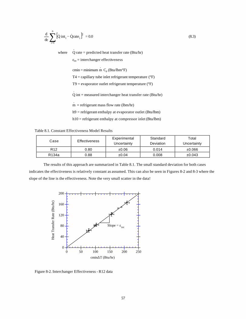
57

[ ]∑=

−ε

n

1i

2ii rateQintQ

dd && = 0.0 (8.3)

where Q. rate = predicted heat transfer rate (Btu/hr)

εint = interchanger effectiveness

cmin = minimum m. Cp (Btu/lbm°F)

T4 = capillary tube inlet refrigerant temperature (°F)

T9 = evaporator outlet refrigerant temperature (°F)

Q. int = measured interchanger heat transfer rate (Btu/hr)

m. = refrigerant mass flow rate (lbm/hr)

h9 = refrigerant enthalpy at evaporator outlet (Btu/lbm)

h10 = refrigerant enthalpy at compressor inlet (Btu/lbm)

Table 8.1. Constant Effectiveness Model Results

Case Effectiveness Experimental Uncertainty

Standard Deviation

Total Uncertainty

R12 0.80 ±0.06 0.014 ±0.066 R134a 0.88 ±0.04 0.008 ±0.043

The results of this approach are summarized in Table 8.1. The small standard deviation for both cases

indicates the effectiveness is relatively constant as assumed. This can also be seen in Figures 8-2 and 8-3 where the

slope of the line is the effectiveness. Note the very small scatter in the data!

0

40

80

120

160

200

0 50 100

Hea

t Tra

nsfe

r Rat

e (B

tu/h

r)

150 200 250

Slope = εint

cmin∆T (Btu/hr)

Figure 8-2. Interchanger Effectiveness - R12 data

58

0

40

80

120

160

200

0 50 100

Hea

t Tra

nsfe

r Rat

e (B

tu/h

r)

150 200

Slope = εint

cmin∆T (Btu/hr)

Figure 8-3. Interchanger Effectiveness - R134a

Since the effectiveness is nearly constant, it would be expected that the constant effectiveness model would

do a good job at predicting interchanger heat transfer. Figures 8-4 and 8-5 compare the predicted interchanger heat

transfer rates to the measured rates. The model is able to predict the heat transfer rates to within ±3.0% for the R12

data and ±5.0% for the R134a data.

40

60

80

100

120

140

160

Pred

icte

d In

tege

rcha

nger

Hea

t Tra

nsfe

r Rat

e(B

tu/h

r)

180

40 60 80 100 120 140 160Measured Interchanger Heat Transfer Rate

(Btu/hr)

180

Figure 8-4. R12 Interchanger Heat Transfer - Constant Effectiveness Model

59

20

40

60

80

100

120

140

160

180

Pred

icte

d In

terc

hang

er H

eat T

rans

fer R

ate

(Btu

/hr)

20 40 60 80 100 120 140 160 180

Measured Interchanger Heat Transfer Rate(Btu/hr)

Figure 8-5. R134a Interchanger Heat Transfer - Constant Effectiveness Model

8.3 Constant UA Model Although the constant effectiveness model does a very good job at predicting interchanger heat transfer, it

can not exp lain why the effectiveness of the interchanger using R134a is 10% higher than for R12. To explore this

question, it is necessary to look at the overall heat transfer coefficient for the interchanger. This quantity is

dependent on fluid properties which may account for the difference.

It is assumed that the overall heat transfer coefficient for the interchanger is constant. The UA for the

interchanger can be determined from an effectiveness-NTU relation for a simple counterflow heat exchanger [2] given

by Equation 8.4. By substituting this expression into Equation 8.1, the rate equation based on UA can be compared

to the measured heat transfer rate. Equation 8.5 was solved to determine the best UA value for all the data points.

εi = 1 - e

(-UAint/cmini) (1-Ri)

1 - Ri e(-UAint/cmini) (1-Ri)

i = 1,n (8.4)

where Ri = cmini/cmaxi

cmax = maximum m. Cp (Btu/lbm°F)

[ ]∑=

−ε−δ

δn

1i

2iiiii

int)9T4T(mincintQ

UA& = 0.0 (8.5)

The results for this model are summarized in Table 8.2. The overall heat transfer coefficient for the R12 data

is 10% higher than for the R134a data. This result at first does not seem consistent with the results in Table 8.1. A

higher overall heat transfer coefficient should relate to a higher effectiveness. However, the heat capacity rates are

significantly different. If the UA's in Table 8.2 are substituted into Equation 8.4 along with nominal heat capacity

rates for both data sets, the effectiveness is predicted to be 0.82 for the R12 data and 0.89 for the R134a data. This is

consistent with the results in Table 8.1.

60

Table 8.2. Constant Overall Heat Transfer Coefficient Model Results

Case UAint

(Btu/hr°F) Uncertainty (Btu/hr°F)

Standard Deviation (Btu/hr°F)

Total Uncertainty (Btu/hr°F)

R12 6.14 ±1.4 0.12 ±1.42 R134a 5.59 ±1.1 0.30 ±1.25

To see if the difference in the overall heat transfer coefficients can be attributed to fluid properties, it is

necessary to separate the overall heat transfer coefficient into its constituent parts. Equation 8.6 relates the overall

heat transfer coefficient for the interchanger to from left to right: the capillary tube convective resistance, the wall

resistance, and the suction line convective resistance. This expression can be simplified by first assuming the wall

resistance is negligible. Second, two phase flow exists inside most of the capillary tube. Since two phase flow

convective coefficients are at least an order of magnitude higher than forced convective coefficients, the first term in

Equation 8.6 is assumed small and can be neglected. Making these assumptions reduces Equation 8.6 to Equation 8.7.

1UAint

= 1

hcapAcap + Rw +

sucsucAh1

(8.6)

where hcap = capillary tube side convective film coefficient

Acap = heat transfer surface area on capillary tube side

Rw = wall resistance

hsuc = suction side film coefficient

Asuc = heat transfer surface area on suction side

UAint ˜ h sucAsuc (8.7)

The suction side film coefficient can be estimated from the Dittus-Boelter equation given by Equation 8.8 [3].

Table 8.3 lists the film coefficients along with the ranges of the Reynolds number and Prandtl number for both

refrigerants. The ratio of the film coefficients should be equal to the ratio of the overall heat transfer coefficients

because the surface area is constant. The ratio of the R12 film coefficient to the R134a film coefficient is 1.23 while the

ratio of the overall heat transfer coefficients is 1.1. Therefore, the same trend is predicted by the theoretical equations.

However, the discrepancy between the two is probably the result of neglecting the other resistances in Equation 8.6.

hsuc = 0.023Re0.8Pr0.4

D

k suc (8.8)

where Re = Reynolds number of gas

Pr = Prandtl number of gas

ksuc = thermal conductivity of gas

Table 8.3. Internal Suction Line Convective Film Coefficients

Case Reynolds Number Prandtl Number Average Film

Coefficient (Btu/hr-ft2°F)

R12 36257 to 44409 0.817 to 0.829 28.3 R134a 18775 to 22557 0.719 to 0.736 23.0

61

If Equation 8.6 is rewritten in the form of Equation 8.9, it is possible to estimate the constant A which

contains both the assumed constant wall resistance and capillary tube resistance. Using the film coefficient for R12

from Table 8.3 and an estimated suction line length of 62 in. which corresponds to a surface area of 0.296 ft2, the value

of A is 0.0435 hr-ft2°F/Btu. Using this value for A, Equation 8.9 predicts the R134a overall heat transfer coefficient to

be 5.3 Btu/hr-ft2°F which is within 5.5% of the value given in Table 8.2.

1UAint

= A + sucsucAh

1 (8.9)

Therefore Equation 8.9 can be used to predict at least relative changes in the overall heat transfer coefficient

for the interchanger. However, note that there is a good deal of uncertainty in the values in Table 8.2. As a result

Equation 8.9 should be used with caution.

Figures 8-6 and 8-7 compare the predicted interchanger heat transfer using the constant UA model to the

measured values. The constant UA model is able to predict the interchanger heat transfer to within ±5% for the R12

data and ±4% for the R134a data. These are essentially the same errors as for the constant effectiveness model.

Therefore for these data sets it appears that both models work equally well.

40

60

80

100

120

140

160

180

Pred

icte

d In

terc

hang

er H

eat T

rans

fer R

ate

(Btu

/hr)

40 60 80 100 120 140 160 180Measured Interchanger Heat Transfer Rate

(Btu/hr)

Figure 8-6. R12 Interchanger Heat Transfer - Constant UA Model

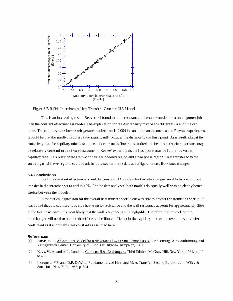
62

20

40

60

80

100

120

140

160

180

Pred

icte

d In

terc

hang

er H

eat T

rans

fer

(Btu

/hr)

20 40 60 80 100 120 140 160 180

Measured Interchanger Heat Transfer(Btu/hr)

Figure 8-7. R134a Interchanger Heat Transfer - Constant UA Model

This is an interesting result. Reeves [4] found that the constant conductance model did a much poorer job

than the constant effectiveness model. The explanation for the discrepancy may be the different sizes of the cap

tubes. The capillary tube for the refrigerator studied here is 0.004 in. smaller than the one used in Reeves' experiments.

It could be that the smaller capillary tube significantly reduces the distance to the flash point. As a result, almost the

entire length of the capillary tube is two phase. For the mass flow rates studied, the heat transfer characteristics may

be relatively constant in this two phase zone. In Reeves' experiments the flash point may be further down the

capillary tube. As a result there are two zones: a subcooled region and a two phase region. Heat transfer with the

suction gas with two regions could result in more scatter in the data as refrigerant mass flow rates changes.

8.4 Conclusions Both the constant effectiveness and the constant UA models for the interchanger are able to predict heat

transfer in the interchanger to within ±5%. For the data analyzed, both models do equally well with no clearly better

choice between the models.

A theoretical expression for the overall heat transfer coefficient was able to predict the trends in the data. It

was found that the capillary tube side heat transfer resistance and the wall resistance account for approximately 25%

of the total resistance. It is most likely that the wall resistance is still negligible. Therefore, future work on the

interchanger will need to include the effects of the film coefficient in the capillary tube on the overall heat transfer

coefficient as it is probably not constant as assumed here.

References [1] Purvis, B.D., A Computer Model for Refrigerant Flow in Small Bore Tubes, Forthcoming, Air Conditioning and

Refrigeration Center, University of Illinois at Urbana-Champaign, 1992.

[2] Kays, W.M. and A.L. London., Compact Heat Exchangers, Third Edition, McGraw-Hill, New York, 1984, pp. 11 to 49.

[3] Incropera, F.P. and D.P. DeWitt., Fundamentals of Heat and Mass Transfer, Second Edition, John Wiley & Sons, Inc., New York, 1985, p. 394.

63

[4] Reeves, R.N., Modeling and Experimental Parameter Estimation of a Refrigerator/Freezer System, Air Conditioning and Refrigeration Center, University of Illinois at Urbana-Champaign, 1992, pp. 30 to 41.

64

Chapter 9: Evaporator Parameter Estimation

9.1 Overview The model for the evaporator is based in part on the work by Reeves [1]. Reeves evaluated the approach

used by DOE and ADL [2,3] and found that modeling the evaporator as containing all two phase liquid from inlet to

outlet did not do a very good job at predicting evaporator heat transfer. This was particularly true for cases where the

evaporator had a significant amount of superheat at the exit. This simple model was markedly improved by splitting

the evaporator into a two phase section and a superheated section.

Reeves used effectiveness-NTU relations [4] with the assumption that the overall conductances contained

in these relations were constants. Once the heat exchanger effectiveness was determined for each section, the

appropriate rate equations were then solved to predict heat transfer from the two phase and superheated sections.

Reeves found that the conductance for the two phase section was 14 times larger than in the superheated section for

his R12 data.

These constant conductances given by Equation 9.1 and 9.2 are a combination of internal and external

resistances to heat transfer. The total resistance to heat transfer, which is the inverse of the overall conductance, is

given by Equation 9.3 [5] where the x refers to either the two phase or superheated section. The terms on the right

side of Equation 9.3 are from left to right: the resistance to heat transfer on the air side, the resistance of the

evaporator tube wall, and the resistance to heat transfer on the refrigerant side. The assumption of constant

conductances is good if the air side and refrigerant side convective film coefficients in Equation 9.3 are constant. The

model should also work if the air side resistance is held constant by keeping the air side volumetric flow rate constant

and the magnitude of the air side resistance is much larger than the other resistances. Under these conditions,

variations in the refrigerant side resistance have little impact on the overall conductance. As a result the overall

conductance is again constant. Note that the area ratios in Equation 9.3 are also constants.

1Usup

= constant (9.1)

1U2ph

= constant (9.2)

where Usup = conductance for the superheated evaporator section

U2ph = conductance for the two phase evaporator section

1Ux

= Ax/Ao

ho +

Axln(ro/ri)

2πLk +

i

ix

hA/A

(9.3)

where Ux = overall conductance based on A x

Ax = arbitrary surface area

ho = air side convective film coefficient

Ao = effective air side surface area

ro = outside radius of evaporator tube

ri = inside radius of evaporator tube

L = length of a given evaporator section

65

k = thermal conductivity of tube

hi = refrigerant side convective film coefficient

Ai = effective refrigerant side surface area

Further, if the air side resistance had dominated the heat transfer process in both sections of Reeve's

evaporator, it would be expected that the conductances for each section would have been nearly equal. However, the

large difference between the two conductances suggests the refrigerant side must be having an impact on the overall

conductance. Rather than assume constant conductances , Reeve's model may be improved by making the overall

conductances functions of the internal film coefficients which vary as functions of mass flow rate and refrigerant

properties.

For the data sets considered here, the evaporator air flow rate was held constant. The air side convective

film coefficient can then be assumed to be constant if property variations in the Reynolds number and Prandtl

number are neglected. This assumption is good for the 0°F to 60°F range of evaporator air temperatures considered.

With these assumptions Equation 9.3 can be written in the form of Equations 9.4 and 9.5. The constant B1, which is

the same for both sections, represents the constant air side resistance plus the assumed constant wall resistance .

The constant B2 is the ratio of the surface area Ax to the refrigerant side surface area A i in Equation 9.3. The

conductances are now functions of the internal film coefficients.

1Usup

= B1 + suph

B2 (9.4)

1U2ph

= B1 + ph2h

B3 (9.5)

where hsup = superheated section refrigerant film coefficient

h2ph = two phase section refrigerant film coefficient

Both the constant conductance model and the variable conductance model will be considered for the R12

and R134a data sets. However, before these conductances can be found, the volumetric air flow rate must be

determined. This quantity is required to evaluate the effectiveness- NTU relations.

9.2 Evaporator Volumetric Flow Rate The volumetric air flow rate across the evaporator was estimated by setting air side and refrigerant side heat

transfers across the evaporator equal to each other. Equation 9.6 lists the relation used. The refrigerant side enthalpy

difference shown is not across the evaporator but rather across the interchanger. It is assumed that the interchanger

is adiabatic relative to the environment. Under this condition the enthalpy difference (h10 - h4) is equal to that across

the evaporator, (h9-h7).

ρCp60V. e∆T = m

. (h10 - h4) = Q

. e (9.6)

V. e = volumetric flow rate (ft3/min)

ρ = density of air (lbm/ft3)

Cp = specific heat of air (Btu/lbm°F)

66

∆T = temperature difference across evaporator (°F)

m. = refrigerant mass flow rate (lbm/hr)

h10 = refrigerant enthalpy at compressor inlet (Btu/lbm)

h4 = refrigerant enthalpy at capillary tube inlet (Btu/lbm)

Q. e = evaporator heat transfer rate (Btu/hr)

The air temperatures at the inlet and outlet of the evaporator unfortunately are not directly measurable. The

return air from the freezer compartment and the fresh food compartment mix right at the bottom of the evaporator coil

as shown in Figure 9-1. Air temperature measurements with a thermocouple couple array mounted to the sheet metal

defrost heater shroud, which is just below the coil, revealed large temperature fluctuations. The same fluctuations

would be expected to occur at the outlet to the evaporator. These air temperatures were too uncertain to use so other

points had to be chosen.

Freezer Compartment

Fresh Food Compartment

Freezer Return Air

Freezer Supply Air

Evaporator Coil

Evaporator Fan

Fresh Food Supply Air

Fresh Food Return Air

Figure 9-1. Refrigerator Evaporator Air Flow Patterns

The inlet air temperature to the evaporator was determined from Equation 9.7. This is simply a mixing

equation for the two evaporator return air streams. In this equation the freezer return air temperature, Tfz, and the

fresh food return air temperature, Tff, are both steady temperatures compared to the evaporator inlet. As a result a

much better estimate of the average mixed air temperature at the inlet to the evaporator can be made. Note that in this

equation the air mass flow rates are as yet unknown.

m. fz h(Tfz) + m

. ff h(Tff) = m

. a h(Tma) (9.7)

where m. fz = mass flow rate of air returning from freezer (lbm/hr)

h(Tfz) = freezer return air enthalpy (Btu/lbm)

67

Tfz = freezer return air temperature (°F)

m. ff = mass flow rate of air from the fresh food compartment (lbm/hr)

h(Tff) = fresh food compartment return air enthalpy (lbm/hr)

Tff = fresh food compartment return air temperature (°F)

m. a = mass flow of mixed air across evaporator (lbm/hr)

h(Tma) = mixed air enthalpy (Btu/lbm)

Tma = mixed air temperature (°F)

The evaporator outlet air temperature was determined by considering an energy balance across the

evaporator fan given by Equation 9.8. In this equation both the fan outlet air temperature and the fan power are

measured. However, as in Equation 9.7, the mass flow rate of air is still not known.

3.413P. fan = m

. a Cp (Tfanout - Taevapout) (9.8)

where P. fan = evaporator fan power (W)

m. a = mass flow rate of air across evaporator (lbm/hr)

Cp = specific heat of air (Btu/lbm°F)

Tfanout = air temperature downstream of evaporator fan (°F)

Taevapout = evaporator outlet air temperature (°F)

Equations 9.6, 9.7 and 9.8 form a system of three equations in six unknowns. To solve the system, three more

equations are required. Two more equations come from applying conservation of mass to the return air streams and

relating the mass flow rate of air across the evaporator to the volumetric flow rate. Equation 9.9 and 9.10 show these

relations. The last equation needed comes from the application of non-linear least squares to find the best estimate of

the volumetric flow rate. Equation 9.11 compares the calculated evaporator heat transfer based on the air side to the

measured heat transfer from the refrigerant side. The best estimate of the volumetric flow rate occurs when the

derivative of this function with respect to V. e is zero.

m. a = m

. fz + m

. ff (9.9)

m. a = ρ60V

. e (9.10)

[ ]2

)4h10h(m)TaevapoutTma(V60CeV

n

1i

iiiiiepii∑=

−−−ρδ

δ &&& = 0.0 (9.11)

Equation 9.12 defines the ratio of the freezer air mass flow rate to the total across the evaporator. This

should be constant and is required for the refrigerator system model [6]. Solving Equation 9.13 yields the best

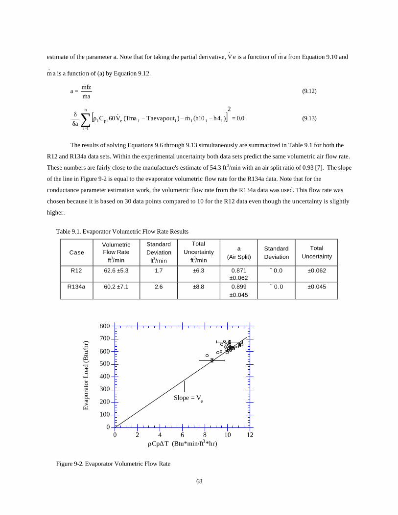
68

estimate of the parameter a. Note that for taking the partial derivative, V. e is a function of m

. a from Equation 9.10 and

m. a is a function of (a) by Equation 9.12.

a = amfzm

&&

(9.12)

[ ]2

)4h10h(m)TaevapoutTma(V60Ca

n

1i

iiiiiepii∑=

−−−ρδδ && = 0.0 (9.13)

The results of solving Equations 9.6 through 9.13 simultaneously are summarized in Table 9.1 for both the

R12 and R134a data sets. Within the experimental uncertainty both data sets predict the same volumetric air flow rate.

These numbers are fairly close to the manufacture's estimate of 54.3 ft3/min with an air split ratio of 0.93 [7]. The slope

of the line in Figure 9-2 is equal to the evaporator volumetric flow rate for the R134a data. Note that for the

conductance parameter estimation work, the volumetric flow rate from the R134a data was used. This flow rate was

chosen because it is based on 30 data points compared to 10 for the R12 data even though the uncertainty is slightly

higher.

Table 9.1. Evaporator Volumetric Flow Rate Results

Case Volumetric Flow Rate

ft3/min

Standard Deviation

ft3/min

Total Uncertainty

ft3/min

a (Air Split)

Standard Deviation

Total Uncertainty

R12 62.6 ±5.3 1.7 ±6.3 0.871 ±0.062

˜ 0.0 ±0.062

R134a 60.2 ±7.1 2.6 ±8.8 0.899 ±0.045

˜ 0.0 ±0.045

0

100

200

300

400

500

600

700

800

Eva

pora

tor L

oad

(Btu

/hr)

0 2 4 6 8 10 12

Slope = Ve

ρCp∆T (Btu*min/ft3*hr)

Figure 9-2. Evaporator Volumetric Flow Rate

69

9.3 Constant Conductance Model To determine the conductances based on Equations 9.1 and 9.2 for both the two phase and superheated

sections of the evaporator, the system of Equations 9.14 through 9.28 were solved. These equations were solved by

the optimization program described in Chapter 5. One of the objective functions that was minimized is given by

Equation 9.14, which is the difference between the measured heat transfer on the refrigerant side and that calculated

from the rate equation.

Minimizee [ ]2

)U,U(erateQeQn

1i

ph2supii∑=

− && (9.14)

Subject to:

Q. eratei = Qe

. supratei + Q

. e2phratei i = 1,n (9.15)

Q. esupratei = esupi cmini (Tsupi - T7i) i = 1,n (9.16)

esupi = 1 - e

-Usup asupi

cmini (1+cmini/casupi)

1 + (cmini/casupi) i = 1,n (9.17)

Q. e2phratei = 1 - e

(-U2ph a2phi/ca2phi) ca2phi (Tmai - T7i) i = 1,n (9.18)

Q.e2phi

Q.ei

= Q.e2phratei

Q.eratei

i = 1,n (9.19)

aevap = asupi + a2phi i = 1,n (9.20)

Q. ei = w

. i (h10i - h4i) i = 1,n (9.21)

Q. esupi = w

. i (h9i - h8satvapi) i = 1,n (9.22)

Q. ei = Q

. e2phi + Q

. esupi i = 1,n (9.23)

ca2phi = caevapi if a2phi/aevap >= 0.5 i = 1,n (9.24) = caevapi (2 a2phi/aevap) if a2phi/aevap < 0.5

casupi = caevapi if a2phi/aevap <= 0.5 i = 1,n (9.25) = caevapi (2 asupi/aevap) if a2phi/aevap > 0.5

Tsupi = Tmidi if a2phi/aevap >= 0.5 i = 1,n (9.26) = Tma if a2phi/aevap < 0.5

Tmidi = Tma - Q.2phpartialicaevapi

i = 1,n (9.27)

Q.2phpartiali =

1 - e

-0.5 U2ph aevap

caevapi caevapi (Tmai - T7i)

i = 1,n (9.28)

70

where Q. erate = predicted heat transfer rate from the evaporator (Btu/hr)

Q. esuprate = predicted heat transfer rate from superheated section (Btu/hr)

Q. e2phrate = predicted heat transfer rate from two phase section (Btu/hr)

esup = effectiveness of superheated section

cmin = heat capacity rate for refrigerant in superheated section (Btu/hr °F)

Tsup = air temperature at inlet to the superheated section (°F)

T7 = saturated refrigerant temperature in evaporator (°F)

Usup = conductance for the superheated section (Btu/hr-ft2 °F)

asup = area of the superheated section (ft 2)

casup = air-side heat capacity rate for superheated section (Btu/hr °F)

U2ph = conductance for the two-phase section (Btu/hr-ft2 °F)

a2ph = area of two-phase section (ft 2)

ca2ph = air-side heat capacity rate for two phase section (Btu/hr °F)

caevap = air-side heat capacity rate for the evaporator (Btu/hr °F)

Tma = mixed air temperature at inlet to the evaporator (°F)

aevap = total surface area of the evaporator (ft2)

Q. e = measured refrigerant heat transfer from the evaporator (Btu/hr)

Q. e2ph = measured refrigerant heat transfer from the two-phase section (Btu/hr)

Q. esup = measured refrigerant heat transfer from the superheated section (Btu/hr)

w. = refrigerant mass flow rate (lbm/hr)

h4 = refrigerant enthalpy at the inlet to the cap-tube (Btu/lbm)

h8satvap = saturated vapor enthalpy in the evaporator (Btu/lbm)

h9 = refrigerant enthalpy at the exit of the evaporator (Btu/lbm)

h10 = refrigerant enthalpy at the compressor inlet (Btu/lbm)

Tmid = air temperature after first row of the evaporator coil (°F)

Q. 2phpartial = heat transfer from first row of coil if all two phase (Btu/hr)

Another objective function given by Equation 9.29 was also used to see if this objective function could

provide more accurate estimates than Equation 9.14. Note that T9 is measured in the lab. Further, the heat transfer

rate for the superheated section comes from the solution of Equations 9.15 to 9.28.

Objective Function = [ ]2

9Tcalc9Tn

1i

i∑=

− (9.29)

where

71

T9calc i = T7i + Qe.

suprateicmini

i = 1,n (9.30)

To help visualize the solution process, Figure 9-3 shows a flow chart for the equations using the objective

function given by Equation 9.29. The labeled arrows represent inputs. The quantities inside the boxes are variables

that are calculated from the inputs.

mrh10h4

h9h8

mr

Iterate Qe2phrate

& a2ph

Tma

T7ca2ph

T7Tmacmincasup

Qesuprate

asupaevap Qerate

Qe

Qesup

Qe2ph

Qe2phrate Qerate

Qe2ph Qe=

T7

cminT9calc

T9

Fix Usup

Fix U2ph

T9 - T9calc

Figure 9-3. Evaporator Equation Flow Diagram

It should be noted that the calculated evaporator exit temperature, T9calc, is not totally independent of the

measured temperature, T9. The loss of independence occurs as a result of not knowing the enthalpy of the refrigerant

at the evaporator inlet. In its place the enthalpies h10, h4 and h9 must be used. Since h9 is a function of measured T9,

the equations are not totally independent. The effect the loss of independence has on the parameter estimation

process will be discussed later.

The equations shown in Figure 9-3 are not the only possible set. One variation is to replace Equation 9.19

with an expression that sets the two phase heat transfer rate equal to the measured refrigerant side value. Computer

runs were made with this set of equations and it was found that it made little difference in the estimated parameters.

This is reasonable since multiplying Equation 9.19 through by the nearly equal total rate and measured evaporator

heat transfers yields the same expression. It is also possible to replace the measured heat transfer from the evaporator

given by Equation 9.21 with an equivalent expression based on the refrigerator cabinet load (Refer to Appendix B).

72

However, for this refrigerator the cabinet load was not known because of the uncertainty introduced by the door

heater.

Some other details about the equations should also be mentioned. The expression for the effectiveness for

the two phase section in Equation 9.18 is independent of geometry. However, the effectiveness equation for the

superheated section is not. Figure 9.4 illustrates the geometry of the evaporator coil. The coil is essentially two

helical coils with spine fins in the inside of the helices. The first obvious choice is to model the superheated section

as a crossflow heat exchanger. However, it was found that this form did not show a minimum in the objective function

for finite values of the conductances. Many other forms were tried but the only effectiveness equation that would

work was for parallel flow. However, for a typical ratio of cmin/casup equal to 0.038 the various effectiveness

equations yield nearly equivalent results [4]. Apparently there must be enough variation in the different expressions

to make a difference in the objective function.

An explanation of the temperature Tsup and the terms ca2ph and casup is needed. The air temperature at the

inlet to the superheated section, Tsup, can be either the mixed air temperature at the inlet to the evaporator or some

lower temperature air off the first row of the coil. In the case shown in Figure 9-4, the superheated section does not

see Tma. Instead it sees the temperature after the first row, Tmid, determined by Equation 9.27. Equation 9.28

calculates the heat transfer from the first row of the coil needed in Equation 9.27 using the best estimate of the

conductance for the two phase section.

Refrigerant Inlet

Refrigerant Outlet

Evaporator Air Inlet - Tma

Two Phase Refrigerant

Superheated Refrigerant

Figure 9-4. Evaporator Coil Geometry

It is also possible, and indeed for most of the R134a data it is the case, that the two phase section occupies

less than half of the coil. In this situation, the superheated section sees the inlet air temperature to the evaporator.

This is the temperature that should then be used in Equation 9.16. It was found that if these geometric considerations

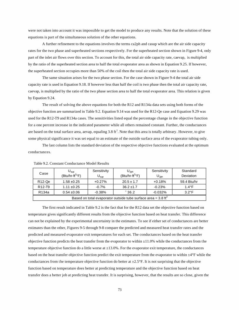
73

were not taken into account it was impossible to get the model to produce any results. Note that the solution of these

equations is part of the simultaneous solution of the other equations.

A further refinement to the equations involves the terms ca2ph and casup which are the air side capacity

rates for the two phase and superheated sections respectively. For the superheated section shown in Figure 9-4, only

part of the inlet air flows over this section. To account for this, the total air side capacity rate, caevap, is multiplied

by the ratio of the superheated section area to half the total evaporator area as shown in Equation 9.25. If however,

the superheated section occupies more than 50% of the coil then the total air side capacity rate is used.

The same situation arises for the two phase section. For the case shown in Figure 9-4 the total air side

capacity rate is used in Equation 9.18. If however less than half the coil is two phase then the total air capacity rate,

caevap, is multiplied by the ratio of the two phase section area to half the total evaporator area. This relation is given

by Equation 9.24.

The result of solving the above equations for both the R12 and R134a data sets using both forms of the

objective function are summarized in Table 9.2. Equation 9.14 was used for the R12-Qe case and Equation 9.29 was

used for the R12-T9 and R134a cases. The sensitivities listed equal the percentage change in the objective function

for a one percent increase in the indicated parameter while all others remained constant. Further, the conductances

are based on the total surface area, aevap, equaling 3.8 ft2. Note that this area is totally arbitrary. However, to give

some physical significance it was set equal to an estimate of the outside surface area of the evaporator tubing only.

The last column lists the standard deviation of the respective objective functions evaluated at the optimum

conductances.

Table 9.2. Constant Conductance Model Results

Case Usup

(Btu/hr-ft2°F) Sensitivity

Usup U2ph

(Btu/hr-ft2°F) Sensitivity

U2ph Standard Deviation

R12-Qe 1.58 ±0.25 +0.27% 20.5 ± 1.7 +0.18% 59.4 Btu/hr R12-T9 1.11 ±0.25 -0.7% 36.2 ±1.7 -0.23% 1.4°F R134a 0.54 ±0.06 -0.38% ˜ 36.2 -0.032% 3.2°F

Based on total evaporator outside tube surface area = 3.8 ft2

The first result indicated in Table 9.2 is the fact that for the R12 data set the objective function based on

temperature gives significantly different results from the objective function based on heat transfer. This difference

can not be explained by the experimental uncertainty in the estimates. To see if either set of conductances are better

estimates than the other, Figures 9-5 through 9-8 compare the predicted and measured heat transfer rates and the

predicted and measured evaporator exit temperatures for each set. The conductances based on the heat transfer

objective function predicts the heat transfer from the evaporator to within ±11.0% while the conductances from the

temperature objective function do a little worse at ±13.0%. For the evaporator exit temperature, the conductances

based on the heat transfer objective function predict the exit temperature from the evaporator to within ±4°F while the

conductances from the temperature objective function do better at ±2.5°F. It is not surprising that the objective

function based on temperature does better at predicting temperature and the objective function based on heat

transfer does a better job at predicting heat transfer. It is surprising, however, that the results are so close, given the

74

substantial difference between the two sets of conductances. As a result, there is no convincing basis for choosing

one set over the other.

800

850

900

950

1000

Pred

icte

d E

vapo

rato

r Loa

d (B

tu/h

r)

1050

1100

1150

± 13%

1200

800Measured Evaporator Load (Btu/hr)

850 900 950 1000 1050 1100 1150 1200

Figure 9-5. R12 Evaporator Heat Transfer Based on Temperature Objective Function

800

850

900

950

1000

Pred

icte

d E

vapo

rato

r Loa

d (B

tu/h

r)

1050

1100

1150

1200

800 850

Measured Evaporator Load (Btu/hr)

900 950 1000 1050 1100 1150 1200

±11.0%

Figure 9-6. R12 Evaporator Heat Transfer Based on Heat Transfer Objective Function

75

16

20

24

28

32

36

16 20

Pred

icte

d T

9 (°

F)

24 28 32 36

±10.0%

Measured T9 (°F)

Figure 9-7. R12 Evaporator Exit Temperature Based on Temperature Objective Function

16

20

24

28

32

Pred

icte

d T

9 (°

F)

36

16 20 24 28 32 36

±15.0%

Measured T9 (°F)

Figure 9-8. R12 Evaporator Exit Temperature Based on Heat Transfer Objective Function

However, there must be an explanation for the lack of sensitivity of the results to the values of the estimated

conductances. To begin to understand this difference, it is helpful to make contour plots of both objective functions.

Figure 9-9 shows the objective function for the R12 data based on heat transfer. For this plot, all the predicted heat

transfer rates should fall within two standard deviations of the optimum value. Two standard deviations for this

objective function is equivalent to a squared error of 113,000. From Figure 9-9, the contour line corresponding to this

76

squared error encompasses a range of two phase and superheated conductances. The two phase conductance

ranges from 18 to 40 Btu/hr-ft2°F and the superheated conductance ranges from 1.2 to 1.9 Btu/hr-ft2°F.

1

1.2

1.4

1.6

1.8

2

2.2

18 20 22 24 26 28 30 32 34 36 38 40

Usu

p

U2ph

0

50000

100000

150000

200000

250000

300000

350000

400000

Figure 9-9. Contour Plot of R12 Objective Function Based on Heat Transfer

The contour plot of the objective function based on temperature is shown in Figure 9-10. For this plot, all

the predicted evaporator exit temperatures should fall within two standard deviations of the optimum. Two standard

deviations for this objective function is equivalent to a squared error of 63. This contour line encompasses a range of

conductances. For the range of superheated conductances from 0.9 to 1.4 , the two phase conductance ranges from

24 to 78.

77

1820222426283032343638404244464850

0.8 0.9 1 1.1 1.2 1.3 1.4

U2p

h

Usup

0

10

20

30

40

50

60

70

80

90

100

Figure 9-10. Contour Plot of R12 Objective Function Based on Temperature

The fundamental question posed by these contour plots is why can the assumed constant conductances for

both objective functions apparently vary over such a large range and still give reasonable results as shown in

Figures 9-5 through 9-8? The answer lies in the form of the objective function and the number of independent

measurements that are available.

Each rate equation contains a conductance and associated area. A given heat transfer rate can be predicted

from the rate equation for a large conductance and small area, or vice versa. The problem with Equations 9.15 through

9.28 is the fact the areas for each zone are not known. Therefore, the conductances and areas need to be fully

constrained. If the areas were known then the comparison of the heat transfer rates with the measured heat transfers

would pin down the conductances.

Since the zone areas are not known this information must come from some other source. The other source is

indirectly Equation 9.19. This ratio helps to constrain the possible range of conductances and areas. However, in the

process of using this equation, some measured quantities are used in both terms of the objective function resulting in

a loss of independence in the equation set. In the objective function given by Equation 9.14, the measured

evaporator heat transfer is used in the rate equations through Equation 9.19. For the objective function given by

Equation 9.29, the measured temperature T9 is also used in the process of calculating T9calc through Equation 9.19.

The penalty to be paid for even a partial loss of independence in the equation set is an inability to independently

estimate the two conductances.

78

A truly independent set of equations can be obtained from independent measurements of the refrigerator

cabinet load. The cabinet load along with the other power inputs into the cabinet can be used to determine the

volumetric air flow rate across the evaporator. Using this air side volumetric flow rate, the evaporator load could be

determined from temperature measurements of the return air streams from the freezer and fresh food compartments

and the evaporator fan outlet. The objective function can then be based on making a comparison between an air side

evaporator heat transfer and the rate equations. The refrigerant side measurements can be used to eliminate the areas

from Equations 9.17 and 9.18, thus eliminating the need for Equation 9.19.

Unfortunately for the refrigerator studied, the cabinet load was not known because of the uncertainty

introduced by the door heater. However, work just recently completed by Boughton [8] on the heat transfer into the

refrigerator cabinet around the door flanges and from the door heater etc. may allow determining the cabinet load.

The solution process just described may yet allow the determination of the conductances from the measured data

sets.

Total Squared Error

2004006008001000120014001600

0200400600800

1000120014001600

Usup

0.2 0.4 0.6 0.8 1

U2ph

5046

4238

3430

2622

1814

10

Figure 9.11. Contour Plot of R134a Objective Function Based on Temperature

The discussion up to this point has dealt with the R12 data. For the R134a data, Figure 9-11 shows a three

dimensional contour plot for the objective function based on temperature. The same general trends shown in the R12

data also appear here. The conductance in the superheated section is fairly well defined but the two phase

conductance is uncertain. As Figure 9-12 shows, there is more scatter in the predicted heat transfer than for the R12

data. This may be a result of the conductances varying more for the R134a data than for the R12 data.

79

300

400

500

600

700

800

300 400

Pred

icte

d H

eat T

rans

fer (

Btu

/hr)

500 600 700 800

±20%

Measured Heat Transfer (Btu/hr)

Figure 9-12. Evaporator Heat Transfer - R134a Constant Conductance Model

The lack of total independence in the equation set may not be the only explanation for the differences

between the estimated conductances. It may als o be true that the conductances are varying. Theoretical calculations

show (see Appendix G) that the conductances for the superheated section may be expected to vary by 11% for the

R12 data and 17% for the R134a. In the two phase section, the conductances vary by 2% in the R12 data and 3% in

the R134a data. Further, the two phase conductances are predicted to be much higher than the superheated

conductances as a result of the much lower resistance on the refrigerant side compared to the refrigerant side

resistance in the superheated zone. The same trend is seen in Table 9.2

The differences between the theoretical conductances for R12 and R134a are mainly the result of changes in

mass flow rates. Fluid properties appear to have a much smaller impact [9]. It would be expected that this result also

holds for the estimated conductances in Table 9.2. Indeed the average mass flow rate for the R134a data is half the

average for the R12 data. As a result the conductance should be lower in the R134a case which is the trend shown in

Table 9.2. A similar comparison can not be made for the two phase conductances because the R134a objective

function did not show in minimum for finite values of the two phase conductance. However, the theoretical

calculations show that since the air side resistance dominates in the two phase section, the two phase conductances

for R12 and R134a should be nearly equal. On this basis, the value of the two phase conductance for the R12-T9 can

be used to approximate the two phase conductance for R134a.

The theoretical variation in the conductances are relatively small. However, the straight tube correlations are

only very crude approximations to the helical geometry in the real evaporator. The helical geometry may significantly

alter flow regimes causing large variations in the conductances. Further more uncertainty is probably introduced by

the uneven distribution in the air inlet temperature and its velocity over the coil.

80

9.4 Variable Conductance Model Since the conductances may be varying significantly in the real evaporator, a variable conductance model

may yield better results than a constant conductance model. For the variable conductance model, Equations 9.4 and

9.5 are substituted into Equations 9.17 and 9.18. Since the same equations are used as for the constant conductance

model, the variable conductance model can not be expected to yield quantitative results because of the large

uncertainties introduced by the loss of independence in the equations. However it is worth seeing if this model

qualitatively makes any improvement over the constant conductance model. Equations 9.4 and 9.5 are repeated here

for reference as Equations 9.31 and 9.32. The refrigerant side film coefficients needed in Equation 9.31 and 9.32 are the

same ones used in the theoretical calculations (see Appendix G). Any discrepancies between these values and the

actual film coefficients in the real evaporator should be taken up by the constants.

1Usup

= B1 + suph

B2 (9.31)

1U2ph

= B1 + ph2h

B3 (9.32)

where hsup = superheated section refrigerant film coefficient

h2ph = two phase section refrigerant film coefficient

The first attempt to find a minimum for the R12 data using this model is summarized by Equation 9.33 and

9.34. The standard deviation in the objective function is 1.13°F which is an improvement over the constant

conductance case which has a standard deviation of 1.4°F. Note that the air side resistance, which is the first term on

the right side of Equations 9.34 and 9.35, is equal to the theoretical value of 0.035 Btu/hr-ft2°F given in Appendix G.

1Usup

= 0.0355 + 28.71hsup 1.10 < Usup < 1.31 Btu/hr-ft2°F (9.33)

1U2ph

= 0.0355 + 0.146h2ph 27.9 < U2ph < 28.0 Btu/hr-ft2°F (9.34)

Further the variation in the superheated conductance from 1.10 to 1.31 is within the range of conductances

where the two objective functions in Figures 9-9 and 9-10 overlap. A comparison can also be made with the

theoretically determined conductances. The theoretical superheated conductances vary by 11% which is the slightly

more than half the 19% variation in Equation 9.34. Both these results suggest that the conductance in the

superheated region is affected by the refrigerant side. For the two phase section, the theoretical conductance varies

by 2% which is much larger than the 0.4% variation in Equation 9.35. These results confirm that the overall

conductance in the two phase section is dominated by the air side resistance. Note also that the values of the two

phase conductance fall close to the middle of the range where the two objective functions in Figures 9-9 and 9-10

overlap. The same model given by Equations 9.31 and 9.32 did not show a minimum for finite values of the constants

for the R134a data.

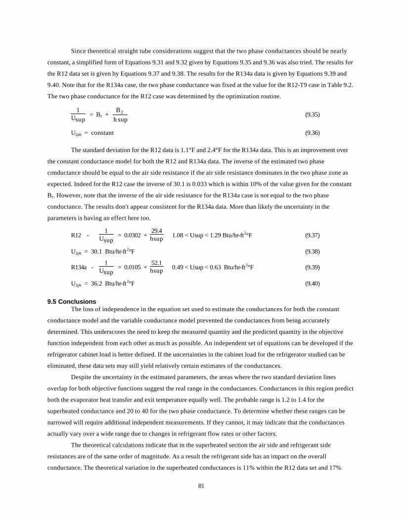
81

Since theoretical straight tube considerations suggest that the two phase conductances should be nearly

constant, a simplified form of Equations 9.31 and 9.32 given by Equations 9.35 and 9.36 was also tried. The results for

the R12 data set is given by Equations 9.37 and 9.38. The results for the R134a data is given by Equations 9.39 and

9.40. Note that for the R134a case, the two phase conductance was fixed at the value for the R12-T9 case in Table 9.2.

The two phase conductance for the R12 case was determined by the optimization routine.

1Usup

= B1 + suph

B2 (9.35)

U2ph = constant (9.36)

The standard deviation for the R12 data is 1.1°F and 2.4°F for the R134a data. This is an improvement over

the constant conductance model for both the R12 and R134a data. The inverse of the estimated two phase

conductance should be equal to the air side resistance if the air side resistance dominates in the two phase zone as

expected. Indeed for the R12 case the inverse of 30.1 is 0.033 which is within 10% of the value given for the constant

B1. However, note that the inverse of the air side resistance for the R134a case is not equal to the two phase

conductance. The results don't appear consistent for the R134a data. More than likely the uncertainty in the

parameters is having an effect here too.

R12 - 1

Usup = 0.0302 +

29.4hsup 1.08 < Usup < 1.29 Btu/hr-ft2°F (9.37)

U2ph = 30.1 Btu/hr-ft2°F (9.38)

R134a - 1

Usup = 0.0105 +

52.1hsup 0.49 < Usup < 0.63 Btu/hr-ft2°F (9.39)

U2ph = 36.2 Btu/hr-ft2°F (9.40)

9.5 Conclusions The loss of independence in the equation set used to estimate the conductances for both the constant

conductance model and the variable conductance model prevented the conductances from being accurately

determined. This underscores the need to keep the measured quantity and the predicted quantity in the objective

function independent from each other as much as possible. An independent set of equations can be developed if the

refrigerator cabinet load is better defined. If the uncertainties in the cabinet load for the refrigerator studied can be

eliminated, these data sets may still yield relatively certain estimates of the conductances.

Despite the uncertainty in the estimated parameters, the areas where the two standard deviation lines

overlap for both objective functions suggest the real range in the conductances. Conductances in this region predict

both the evaporator heat transfer and exit temperature equally well. The probable range is 1.2 to 1.4 for the

superheated conductance and 20 to 40 for the two phase conductance. To determine whether these ranges can be

narrowed will require additional independent measurements. If they cannot, it may indicate that the conductances

actually vary over a wide range due to changes in refrigerant flow rates or other factors.

The theoretical calculations indicate that in the superheated section the air side and refrigerant side

resistances are of the same order of magnitude. As a result the refrigerant side has an impact on the overall

conductance. The theoretical variation in the superheated conductances is 11% within the R12 data set and 17%

82

within the R134a data set. These variations are small and may prevent the separation of the overall conductances into

an air side and refrigerant side component even with an independent set of equations. It might therefore be necessary

to expand the data set by varying the air side volumetric flow rate. Qualitatively, the variable conductance model in

the superheated zone is an improvement over the constant conductance model. However, more research is needed to

determine if the improvement is just a result of adding another degree of freedom to the objective function or whether

the model is actually accounting for the apparent small variations in the superheated conductance.

In the two phase section the air side resistance dominates the refrigerant side resistance. As a result,

variations in the refrigerant side resistance have little impact on the overall conductance. The theoretical variation in

the two phase conductances is only 2% for the R12 data and 3% for the R134a data. This suggests that for this

section, the constant conductance model ought to be sufficient and the same conductance value can be used for

both refrigerants.

However, the possibility remains that the helical geometry of the evaporator actually causes the two phase

resistance to vary substantially as a function of refrigerant mass flow rate, and that the refrigerant side resistance and

flow regimes are highly sensitive to the refrigerant type. Further exploration of these issues will require the use of two

phase flow correlations more complicated than those for straight tubes, and should resolve some of the other issues

raised here.

References [1] Reeves, R.N., Modeling and Experimental Parameter Estimation of a Refrigerator/Freezer System, Air

Conditioning and Refrigeration Center, University of Illinois at Urbana-Champaign, 1992, pp. 30 to 41.

[2] Arthur D. Little, Inc., Development of a High Efficiency Automatic Defrosting Refrigerator/Freezer: Phase I Final Report, ORNL/Sub-7255/2, February 1980.

[3] Arthur D. Little, Inc., Refrigerator and Freezer Computer Model User's Guide, U.S. Department of Energy DE-AC01-78CS20420, November 1982.

[4] Kays, W.M. and A.L. London., Compact Heat Exchangers, Third Edition, McGraw-Hill, New York, 1984, pp. 11 to 49.

[5] Stoecker, W.F. and J.W. Jones., Refrigeration and Air Conditioning, McGraw-Hill, New York, 1986, p. 236.

[6] Porter, K.J., Modeling and Sensitivity Analysis of a Refrigerator/Freezer System, ACRC Technical Report, Air Conditioning and Refrigeration Center, University of Illinois at Urbana-Champaign, forthcoming 1992.

[7] Personal communication., Mr. Martin Zenter, General Electric Company, Appliance Park, Louisville, Kentucky, 40255.

[8] Boughton, B.E., An Investigation of Household Refrigerator Cabinet Loads, Air Conditioning and Refrigeration Center, University of Illinois at Urbana-Champaign, 1992.

[9] Personal communication, Mr. John Wattelet, Air Conditioning and Refrigeration Center, University of Illinois at Champaign-Urbana, Champaign-Urbana, Illinois, 61801.

83

Chapter 10: Conclusions and Recommendations

The purpose of this project was to verify that the component models developed by Reeves [1] are valid for

the refrigerator/freezer studied here and that the models could be extended to handle refrigerants other than R12. For

the heat exchangers, the constant multi-zone conductance models used by Reeves were extended to variable

conductance models to see if they could account for the differences in heat transfer characteristics between R12 and

R134a. In the process several important results were obtained.

For the compressor, the constant overall heat transfer coefficient model for shell heat transfer was verified

for two more reciprocating compressors. A volumetric and isentropic efficiency approach for predicting compressor

performance was investigated as an alternative to the compressor maps used by Reeves. It was found that both the

volumetric efficiency approach and the compressor maps predicted compressor performance equally well. Each

method was able to predict compressor mass flow rate and power consumption to within ±5.0%. The volumetric

efficiency approach has the added advantage of being applicable to a wider range of compressor operating

conditions. In fact, the same compressor calorimeter data used to generate compressor maps can be used to develop

a volumetric and isentropic efficiency model that applies to test conditions outside the evaporating and condensing

temperatures of the original data points. In the future these models should be further validated for other compressor

geometries such as a rotary compressor and compressors that have the shell on the low side of the compressor.

For the condenser, the three-zone constant conductance model developed by Reeves was validated for the

refrigerator/freezer studied. The model was able to predict condenser heat transfer to within ±10.0% for both R12 and

R134a. The attempt to go one step further to a variable conductance model to account for the observed differences

between R12 and R134a revealed that within a given data set the conductances were relatively constant over the

range of refrigerant side test conditions observed. The variation in the conductances was apparently not enough to

allow the air side and refrigerant side components to be separated. It is recommended that the air side volumetric flow

rate be varied so that the effects can be separated. This should yield a variable conductance model capable of

predicting the effects of changing refrigerants.

The reason the conductances appear to be relatively constant is a result of the magnitude of the air

resistance relative to the total resistance to heat transfer. In the two phase section the air side resistance is

theoretically 80% of the total and approximately 50% in the desuperheating section. As a result variations in the

refrigerant side resistance due to varying mass flow rates and properties have little impact in the two phase section of

the condenser and only slight impact on the desuperheating section for the measured refrigerant mass flow rate range

of 7 to 20 lbm/hr. In the subcooled section, the Reynolds number is so small that the flow is laminar for the conditions

tested. As a result, the resistance in this section is expected to be a function of refrigerant properties alone. For the

R134a data set, the refrigerant properties did not vary over a wide enough range to significantly vary the overall

conductance.

For the interchanger, it was verified that a constant effectiveness model does an excellent job at predicting

heat transfer in the interchanger. Interestingly, it was also found that a constant overall heat transfer coefficient

model also does an excellent job. Reeves found that the constant overall heat transfer coefficient model did a much

worse job for his refrigerator/freezer. The refrigerator studied here had a 0.028" I.D. capillary while the one studied by

84

Reeves had a 0.032" capillary tube. Further investigation into the reasons why a change in tube diameter has such a

pronounced effect is warranted as it may yield a better understanding of the interaction between the capillary tube

and suction line. Part of the variation might also be attributed to differences in the locations of the flash point.

For the evaporator it was found that the constant conductance model used by Reeves did not do a very

good job at predicting heat transfer from the evaporator. An investigation into the underlying reasons revealed two

possibilities: either 1) the conductances vary substantially with refrigerant mass flow rate due to the helical geometry

of the evaporator or 2) a much more subtle reason involving the equation set is the cause. In fact, both effects may be

occurring simultaneously. In the process of developing a set of equations on which to base an objective function it is

possible that the same measured quantities can be used twice in both the predicted and measured terms. As a result

the measured and predicted terms are not totally independent of one another. The effect of this loss of independence

is the introduction of more uncertainty into the estimated parameters. However, even with these uncertainties it was

found that the variable conductance model showed an improvement over the constant conductance model for both

R12 and R134a.

Better estimates of the parameters in both models is needed to determine if the variable conductance model

is indeed better. This may still be possible for the R12 and R134a data sets by using an independent set of equations

employing measurements of the refrigerator cabinet load. The cabinet load along with the other power inputs into the

cabinet can be used to determine the volumetric air flow rate across the evaporator. Using this air side volumetric

flow rate, the evaporator load can be determined. Better parameter estimates may be obtained by finding which values

minimize the difference between the measured heat transfer and that calculated by the rate equations. In this case, the

refrigerant side measurements can be used to eliminate the need to know the areas in each zone. The necessary

measurements of cabinet load may be contained in the data sets obtained here to calibrate a recently developed

model of door edge losses. This would remove the uncertainty about the contribution of the door heater and provide

the independent information needed.

In summary, the goal of accurately predicting the effect of alternative refrigerants in domestic

refrigerator/freezers will require better models of the condenser and evaporator than those presented here. On the one

hand it will be necessary to vary airflow rates to obtain a better separation between refrigerant and air-side heat

transfer phenomena. On the other hand it might be possible to simulate performance of a system with fixed air flow

rates by using a constant conductance model of the type presented here for the condenser and suction line heat

exchanger. The same might be possible for the evaporator if the resolution of door heater uncertainties yields the

independent source of measurements required.

References [1] Reeves, R.N., Modeling and Experimental Parameter Estimation of a Refrigerator/Freezer System, Air

Conditioning and Refrigeration Center, University of Illinois at Urbana-Champaign, 1992, pp. 30 to 41.

85

List of References

American Society of Heating, Refrigerating and Air-Conditioning Engineers, Inc., Fundamentals Handbook, ASHRAE, Atlanta, 1989, p. 4.2.

Arthur D. Little, Inc., Development of a High Efficiency Automatic Defrosting Refrigerator/Freezer: Phase I Final Report, ORNL/Sub-7255/2, February 1980.

Arthur D. Little, Inc., Refrigerator and Freezer Computer Model User's Guide, U.S. Department of Energy DE-AC01-78CS20420, November 1982.

Boughton, B.E., An Investigation of Household Refrigerator Cabinet Loads, Air Conditioning and Refrigeration Center, University of Illinois at Urbana-Champaign, 1992.

Camporese, R., G. Bogolaro, G. Cortella, and M. Scattolini. 1991. "Flammable Refrigerants in Domestic Refrigeration.", Proceedings of the XVIII International Congress of Refrigeration, Vol. III, pp. 1175 to 1179.

Coleman, H.W. and W.G. Steele., Experimentation and Uncertainty Analysis for Engineers, John Wiley & Sons, New York, 1989.

Collier, J. G., Convective Boiling and Condensation, Second Edition, McGraw-Hill, New York, 1980, pp. 30 to 35.

Copeland Copeleweld Data Book, Copeland Corporation, Sidney, Ohio (1990).

Dabiri, A.E. and C.K. Rice. 1981. "A Compressor Simulation Model with Corrections for the Level of Suction Gas Superheat.", ASHRAE Transactions,Vol. 87, Part 2, pp. 77 to 782.

Department of Energy. 1979. "Test procedures for central air conditioners, including heat pumps." Federal Register, Vol. 44, No. 249, pp. 76700 to 76723.

Department of Energy. 1989. "Uniform test method for measuring the energy consumption of central air-conditioners." Code of Federal Regulations, Part 430, Subpart B, Appendix M, pp. 101 to 126, January 1.

E.E.S., F-Chart Software, 4406 Fox Bluff Road, Middleton, WI, 53562.

Engineering Analysis of Experimental Data - ASHRAE Guideline 2-1986., (Available from American Society of Heating, Refrigerating and Air-Conditioning Engineers, Inc., 1791 Tullie Circle, N.E., Atlanta, GA 30329).

Goldschmidt, V.W., G.H. Hart, and R. C. Reiner. 1980. "A note on the transient performance and degradation coefficient of a field tested heat pump - cooling and heating mode." ASHRAE Transactions, Vol. 86, Part 2, pp. 368 to 375.

Hara, T., and M. Shibayama, H. Kogure, and A. Ishiyama. 1991. "Computer Simulation of Cooling Capacity for a Domestic Refrigerator-Freezer.", Proceedings of the XVIII International Congress of Refrigeration, Vol. III, pp. 1193 to 1197.

He, X., U.C. Spindler, D.S. Jung, and R. Radermacher. 1992. "Investigation of R-22/R-142b Mixture as a Substitute for R-12 in Single-Evaporator Domestic Refrigerators.", ASHRAE Transactions, Vol. 98, Part 2, 1992.

Incropera, F.P. and D.P. DeWitt., Fundamentals of Heat and Mass Transfer, Second Edition, John Wiley & Sons, Inc., New York, 1985.

Katipamula, S. and D.L. O'Neal. 1991. "Performance degradation during on-off cycling of single-speed heat pumps operating in the cooling mode: experimental results." ASHRAE Transactions, Vol. 97, Part 2, In print.

Kays, W.M. and A.L. London., Compact Heat Exchangers, Third Edition, McGraw-Hill, New York, 1984.

Kempiak, M.J. and R.R. Crawford., Three-Zone Modeling of a Mobile Air Conditioning Condenser, Air Conditioning and Refrigeration Center, Dept. of Mechanical and Industrial Engineering, University of Illinois at Urbana-Champaign, 1992.

Molina, M.J. and F.S. Rowland. 1974. "Stratospheric Sink for Chlorofluoromethanes: Chlorine Atom Catalyzed Destruction of Ozone.", Nature 249: pp. 810 to 812.

Mulroy, W.J. and D.A. Didion. 1985. "Refrigerant migration in a split-unit air conditioner." ASHRAE Transactions, Vol. 91, Part 1A, pp. 193 to 206.

86

Murphy, W.E., and V.W. Goldschmidt. 1979. "The degradation coefficient of a field-tested self-contained 3-ton air conditioner." ASHRAE Transactions, Vol. 85, Part 2, pp. 396 to 405.

Murphy, W.E., and V.W. Goldschmidt. 1984. "Transient response of air conditioners-a qualitative interpretation through a sample case." ASHRAE Transactions, Vol. 90, Part 1B, pp. 997-1008

NAECA. 1987. Public law 100-12, March 17.

Pereira, R.H., L.M. Neto, and M.R. Thiessen. 1991. "An Experimental Approach to Upgrade the Performance of a Domestic Refrigeration System Considering the HFC-134a.",Proceedings of the XVIII International Congress of Refrigeration, Vol. III, pp. 1180 to 1184.

Porter, K.J., Modeling and Sensitivity Analysis of a Refrigerator/Freezer System, ACRC Technical Report, Air Conditioning and Refrigeration Center, University of Illinois at Urbana-Champaign, forthcoming 1992.

Purvis, B.D., A Computer Model for Refrigerant Flow in Small Bore Tubes, Air Conditioning and Refrigeration Center, University of Illinois at Urbana-Champaign, forthcoming 1992.

Reeves, R.N., Modeling and Experimental Parameter Estimation of a Refrigerator/Freezer System, Air Conditioning and Refrigeration Center, Dept. of Mechanical and Industrial Engineering, University of Illinois at Urbana-Champaign, 1992.

Rogers, S. and D.R. Tree. 1991. "Algebraic Modelling of Components and Computer Simulation of Refrigerator Steady-State Operation.", Proceedings of the XVIII International Congress of Refrigeration, Vol. III, pp. 1225 to 1229.

Rohsenow, W.M., "Boiling" in W.M. Rohsenow et al., Eds., Handbook of Heat Transfer Fundamentals , Chapter 12, McGraw-Hill, New York, 1985.

Science. v. 254, no. 5032, 1991.

Stoecker, W.F. and J.W. Jones, Refrigeration and Air Conditioning, McGraw-Hill, New York, 1986.

Stoecker, W.F., Design of Thermal Systems , Third Edition, McGraw-Hill, New York, 1989.

Sugalski, A., D. Jung, and R. Radermacher. 1991. "Quasi-Transient Simulation of Domestic Refrigerators.", Proceedings of the XVIII International Congress of Refrigeration, Vol. III, pp. 1244 to 1249.

True Basic., True Basic, Inc., 39 South Main St., Hanover, N.H., 03755.

United Nations Environmental Programme. 1987. Montreal protocol on substances that deplete the ozone layer. Final act., New York: United Nations.

Vineyard, E.A. 1991. "The Alternative Refrigerant Dilemma for Refrigerator-Freezers: Truth of Consequences.", ASHRAE Transactions, Vol. 97, Part 2, pp. 955 to 960.

Xiuling, C., C. Youhong, X. Deling, G. Yain, and L. Xing. 1991. "A Computer Simulation and Experimental Investigation of the Working Process of a Domestic Refrigerator.", Proceedings of the XVIII International Congress of Refrigeration, Vol. III, pp. 1198 to 1202.

87

Appendix A: Performance Degradation of Domestic Refrigerators during Cyclic Operation

A.1 Overview The intent of this discussion is to investigate the differences between steady-state and cycling performance

of a domestic refrigerator at one test condition. Experimental data were collected for a standard 18 ft3 refrigerator in

both steady-state and cyclic operation. The refrigerator was operated in a controlled environment in an

environmental chamber. Both tests were run at 90°F ambient (chamber temperature) with a refrigerant charge of 7oz.

Note that for these tests the mullion heater was deactivated. The freezer and fresh-food compartment temperature

controls were set at their midpoint positions for the cycling test. The average freezer and fresh-food compartment

temperatures in the cycling test were matched in the steady-state test. Other approaches could be taken to make a

comparison such as running the refrigerator with the same evaporator load for each test. However, maintaining

equivalent temperatures seems the most logical because the purpose of the refrigerator is to maintain a given set-

point temperature.

A.2 Cycling Performance in Heat Pumps and Air-Conditioning Equipment Before discussing results for refrigerators, it is instructive to briefly review the significant amount of work

that has been done in this area on heat pumps and air-conditioning equipment (see for example, Murphy and

Goldschmidt [1], Goldschmidt et al. [2], Murphy and Goldschmidt [3], and Katipamula and O'Neal [4]). The methods

and trends identified should be useful in analyzing and understanding the cyclic performance of domestic

refrigerators.

The approach taken to quantify the efficiency of a heat pump or air conditioner during cyclic operation was

first proposed by the Department of Energy [5].The method involves taking a steady-state efficiency and multiplying

it by a factor that accounts for transient losses caused by cyclic compressor operation. The resulting quantity is

called a Seasonal Energy Efficiency Ratio or SEER. This efficiency should be more representative of the actual

efficiency of a heat pump compared to a steady-state value. To evaluate this quantity, several steady-state tests and

a cycling test are required. DOE [6] defined SEER by Equation 1 where EERB is a steady-state energy efficiency rating

for the heat pump at 82°F outdoor and 80°F indoor ambient conditions and PLF is the part load factor determined at a

cooling load factor or CLF of 50% .

SEER = EERB x PLF(CLF = 50%) (A.1)

The part load factor is defined as the average efficiency of the heat pump during the cooling phase of a

specified cycle test D divided by the efficiency of steady-state test C as given by Equation 2 where t o is the cooling-

process time or on-cycle time. The part load factor indicates how closely the cycling efficiency of the unit approaches

the steady-state value. The cooling load factor or CLF is defined by Equation 3 where Q.(t) D is the instantaneous heat

transfer rate for cyclic operation in test D and Q. ssC is the heat transfer rate for steady-state operation in test C. For

this parameter the integration is performed over the complete cycle time t c. The cooling load factor represents the

ratio of the heat transferred in a cycle to that which could be transferred if the unit ran continuously.

88

PLF = C

t

oD

o

EER

dt)t(EERt1 o

∫ (A.2)

CLF = cC

t

oD

tssQ

dt)t(Qc

&

&∫ (A.3)

An alternative approach that makes use of a degradation coefficient was also given [6] to calculate the part

load factor needed in Equation 1. The degradation coefficient is defined by Equation 4. It was assumed that as the

cooling load factor increased the part load factor would also increase in such a way that the degradation coefficient

would remain constant. Once CD was known at one test point it could be applied to other conditions. Further, with CD

known and CLF set to 0.5, Equation 4 can be solved for the part load factor needed in Equation 1.

CD = CLF1PLF1

−−

(A.4)

Later work by Murphy and Goldschmidt [1] and Goldschmidt et al. [2] has shown that the degradation

coefficient is not constant. Katipamula and O'Neal [4] tested a heat pump in cooling mode with different cycling rates

and percent compressor on-times at constant ambient conditions. They found that the part load factor increased with

percent compressor on-time and decreased with the cycle rate. The degradation in performance was worse at high

cycle rates and low percent compressor on-times. Further, the degradation coefficient varied significantly over the

conditions tested.

Unfortunately there doesn't seem to be a simple relationship between the cycle rate, percent compressor on-

time and the cooling efficiency of a heat pump. However, the trends outlined by Katipamula and O'Neal [4] should

also hold for domestic refrigerators. More work will obviously be needed to fully characterize the relationship

between steady-state and cycling performance of heat pumps and air conditioning equipment.

A.3. Comparison of Steady-State Performance and a "Snapshot" of Cycling Performance Two methods will be used to investigate the differences between cycling and steady-state performance of a

domestic refrigerator. The first method is to make the comparison between the steady-state and cyclic cases by

looking at a point in time where the instantaneous evaporator inlet air temperatures are the same. For this case an

instantaneous coefficient of performance or COP can be compared to the steady-state value where COP is defined as

the ratio of the evaporator load to the system power requirement. The second approach is to compare an average

COP for the cycling case to the steady-state value. Since the cyclic COP is a function of time, an average can be

found by integrating over a complete cycle. Both methods yield valuable insights. The equal evaporator air

temperature approach will be investigated first.

Table A.1 lists the temperatures, pressures, and power requirements for the system when the evaporator

inlet temperature was the same for the cycling and steady-state tests. The cyclic evaporator load was determined

from an air-side energy balance across the evaporator. The same method was applied to the steady-state case.

89

The cyclic COP is 11% lower than the steady-state value which is a significant decrease in the efficiency of

the refrigerator. The cyclic losses appear as a significant loss in evaporator capacity and not in the power

requirement which is equal to the steady-state. To begin to understand why it takes the same amount of power to

move much less heat in the cyclic case, a closer look at the differences between the two tests must be taken.

There is little difference between the steady-state case and this "snapshot" of the cycling case except for

the compressor discharge temp erature, refrigerant temperature at the exit of the evaporator, and the evaporator air

discharge temperature. The decrease in the compressor discharge temperature can be explained by thermal capacity

effects. Since the compressor has a large thermal capacity, it can store a significant amount of energy. During the off-

cycle, the compressor shell transfers heat to the cooler environment. When the compressor resumes operation, the

metal in the compressor can absorb energy from the refrigerant stream until steady-state conditions are reached

between the compressor shell and the environment. This reduces the enthalpy of the refrigerant stream leaving the

compressor resulting in a lower discharge temperature. Note that this effect tends to increase, not decrease, system

efficiency.

Table A.1. Steady-State and Instantaneous Cyclic Performance

Measured Quantity Steady-State Cyclic

Condenser Inlet Pressure (psig) 136 137 Condenser Outlet Pressure (psig) 135 136 Evaporator Inlet Pressure (psig) 3.8 3.8 Evaporator Outlet Pressure (psig) 1.4 1.4 Fresh Food Compartment Temp. (°F) 41.6 39.3 Freezer Compartment Temp. (°F) 3.4 3.4 Evaporator Inlet Air Temp. (°F) 6.7 6.6 Evaporator Outlet Air Temp. (F) -1.6 -0.8 Evaporator Inlet R12 Temp. (°F) -11.3 -11.3 Evaporator Outlet R12 Temp. (°F) -13.8 -8.2 Compressor Suction Inlet Temp. (°F) 86.3 87.9 Compressor Discharge Temp. (°F) 170.1 160.8 Condenser Inlet R12 Temp. (°F) 170.1 160.8 Condenser Outlet R12 Temp. (°F) 112.5 112.7 Capillary Tube Inlet Temp. (°F) 111.7 111.8 Ambient Temperature (°F) 89.8 89.6 Compressor Power (W) 161 163 Evaporator Load - Air Side (W) 170 153 System Power (W) 187 189 COP 0.91 0.81

Evidence for this process can be seen in Figure A-1. An on-cycle and off-cycle are also indicated. For each

cycle the compressor shell experiences a temperature fluctuation of 9°F. The mass of the compressor minus the oil

charge is 18.5 lbm. If it is assumed that all of this mass is steel (neglecting the higher thermal capacitance of the

copper motor windings) and that all of it undergoes the same 9°F temperature fluctuation, 17.3 Btu are stored and

dissipated each cycle. Averaging over the 25.1 minute on-cycle yields 41.4 Btu/hr or 12.1 W. It should also be

90

possible to determine this heat transfer rate from the actual discharge enthalpies for the cycling and steady-state

cases and the refrigerant flow rate which is equal for both cases. Using Equation 5 and a mass flow rate of 12.6 lbm/hr

results in a heat transfer rate of 6.3 W. Although not exactly equal, this value is the same order of magnitude as the

12.1 W calculated previously given the assumptions made. It is therefore probable that the decrease in the discharge

temperature for the cycling case is the result of thermal storage effects in the compressor.

Q. stored = )hh(m cyclingss −& (A.5)

where hss = discharge enthalpy, steady-state

hcycling = discharge enthalpy, cycling

m. = refrigerant flow rate

130

134

138

142

146

150

0

Tem

pera

ture

(°F)

20 40 60 80 100 120 140

OnCycle

OffCycle

Time (min.)

Figure A-1. Compressor Shell Temperature for Cycling Operation

The other main difference between the two cases is in evaporator performance. For the measured

temperature and pressure, the steady-state evaporator has 4 °F of superheat at the exit. Likewise the cycling case has

9.5 °F of superheat, a significant difference. In fact the superheat levels for the cycling case are much higher over

most of the compressor on-cycle. Figure A-2 shows that the evaporator superheat rises to a maximum of 17°F before

slowly decreasing toward the steady-state value. The steady-state superheat level is only reached at the end of the

compressor on-cycle.

91

-20

-15

-10

-5

0

5

10

15

20

Tem

pera

ture

(°F)

0 20 40 60 80 100 120 140Time (min.)

Inlet-R12

Outlet-R12

Superheat

Figure A-2. Superheat in the Cycling Evaporator

High superheat levels greatly reduce the capacity of the evaporator. This explains why the evaporator load

is lower and leaving air temperature is higher for the cycling case than for the steady-state case. However there must

be a reason why the evaporator superheat is higher for the cycling case and the most logical inference is that the

evaporator is starved for refrigerant. It could also be argued that the mass flow rate is lower for the cycling case.

However, since the compressor sees the same inlet and outlet pressures and the same suction temperature, the mass

flow rate through the compressor for the two cases must be nearly the same. Note that the compressor inlet pressure

is the same as the evaporator outlet pressure and the compressor discharge pressure is the same as the condenser

inlet pressure; the line losses being negligible.

The low charge in the evaporator can be explained if when the compressor first turns on a significant

amount of liquid refrigerant is removed from the evaporator and is stored in the condenser or compressor shell for

most of the compressor on-cycle. Murphy and Goldschmidt reported the same type of behavior in an air conditioner

[3]. Qualitative evidence for this can be seen in Figure A-1 and A-3. In Figure A-1 the compressor shell temperature

drops 5°F after the compressor begins operating instead of increasing indicating that liquid refrigerant is entering the

compressor. In Figure A-3 the very sharp drop in suction temperature right after the compressor turns on indicates

liquid refrigerant is drawn from the evaporator into the suction line heat exchanger.

92

20

40

60

80

100

120

Com

pres

sor S

uctio

n Te

mpe

ratu

re (°

F)

0 20 40 60 80 100 120 140Time (min.)

Figure A-3. Compressor Suction Temperature for the Cyclic Case

From the variation in superheat over the entire on-cycle, the refrigerant must migrate back into the

evaporator slowly. For this to occur, the mass flow rate through the capillary tube must be slightly higher than the

mass flow rate through the compressor. In fact if all the 7oz. charge migrated over the entire 25.1 minute on-cycle, the

capillary tube would have to allow approximately 1.0 lbm/hr more mass flow than the compressor or about 8%.

However, high superheat levels in the evaporator result in higher exiting refrigerant temperatures from the evaporator.

Higher evaporator exit temperatures mean less heat transfer in the suction line heat exchanger. Since the capillary

tube is soldered to the suction line, less energy is removed from the liquid refrigerant in the cap-tube. The liquid

refrigerant has a lower density at a higher average temperature which results in a lower mass flow rate for a given

pressure differential across the capillary tube. From this viewpoint, the suction line heat exchanger retards the

redistribution of refrigerant in the system which prevents the system from approaching steady-state efficiency.

A.4 Refrigerant Charge Migration from the Condenser The removal of charge from the evaporator is not the only migration of refrigerant in the system during a

cycle. Refrigerant also migrates from the condenser to the evaporator during the off-cycle. When the compressor

shuts down, the pressure in the condenser decreases as refrigerant bleeds through the capillary tube to the much

lower pressure evaporator. Depending on how this process occurs, heat can also be transferred as a result. This

could be an important additional load on the evaporator in the cycling case. Murphy and Goldschmidt [3] also

discuss this phenomenon.

Two hypothetical migration processes are illustrated in Figure A-4. In case one, refrigerant forms a

continuous column of liquid from the outlet of the condenser to the inlet of the capillary tube. For this situation,

when the compressor stops, the pressure in the condenser forces the liquid refrigerant out of the condenser through

the cap-tube. This would result in additional cooling in the evaporator even though the compressor is not running. If

this process were to occur in a real refrigerator, the migration would not be considered a loss because some cooling

would be accomplished.

93

Condenser

Evaporator

Qcondenser

Tambient

Qevaporator Tfreezer

Door HeaterCapillary Tube

Case 1

Door Heater

Condenser

Evaporator

Qcondenser

Tambient

Qevaporator Tfreezer

Capillary Tube

Case 2

Figure A-4. Hypothetical Refrigerant Migration Processes

In case 2, the column of liquid is not continuous but is broken as the result of drainage back into the

condenser due to gravity and the likely formation of vapor. For this scenario, only vapor is transferred to the

evaporator. Initially the liquid refrigerant in the condenser is above the ambient temperature. However since saturated

conditions exist in the condenser, as the pressure falls so does the refrigerant temperature. Eventually the pressure

drops far enough to cause the refrigerant temperature to drop below the ambient temperature. At this point the

direction of heat transfer from the refrigerant to the environment is reversed and the refrigerant begins to boil. The

heat absorbed in the condenser is transported by refrigerant migration to the evaporator where condensation occurs

transferring the heat into the refrigerator cabinet. For this case, the migration of refrigerant during the off-cycle is a

loss. Note that for both cases it was assumed that the pressure in the condenser was sufficient to keep the discharge

valve on the compressor closed thus preventing flow back through the compressor.

-20

-10

0

10

20

30

40

50

Tem

pera

ture

(°F)

0 20 40 60 80 100 120 140Time (min.)

Fresh Food TemperatureFreezer TemperatureRefrigerant Temp. - Evaporator Inlet

Figure A-5. Effect of Refrigerant Migration on Evaporator Refrigerant Temperature

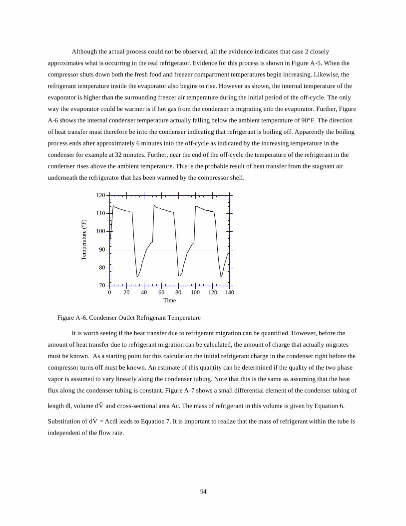
94

Although the actual process could not be observed, all the evidence indicates that case 2 closely

approximates what is occurring in the real refrigerator. Evidence for this process is shown in Figure A-5. When the

compressor shuts down both the fresh food and freezer compartment temperatures begin increasing. Likewise, the

refrigerant temperature inside the evaporator also begins to rise. However as shown, the internal temperature of the

evaporator is higher than the surrounding freezer air temperature during the initial period of the off-cycle. The only

way the evaporator could be warmer is if hot gas from the condenser is migrating into the evaporator. Further, Figure

A-6 shows the internal condenser temperature actually falling below the ambient temperature of 90°F. The direction

of heat transfer must therefore be into the condenser indicating that refrigerant is boiling off. Apparently the boiling

process ends after approximately 6 minutes into the off-cycle as indicated by the increasing temperature in the

condenser for example at 32 minutes. Further, near the end of the off-cycle the temperature of the refrigerant in the

condenser rises above the ambient temperature. This is the probable result of heat transfer from the stagnant air

underneath the refrigerator that has been warmed by the compressor shell.

70

80

90

100

110

120

0 20 40

Tem

pera

ture

(°F)

60 80 100 120 140Time

Figure A-6. Condenser Outlet Refrigerant Temperature

It is worth seeing if the heat transfer due to refrigerant migration can be quantified. However, before the

amount of heat transfer due to refrigerant migration can be calculated, the amount of charge that actually migrates

must be known. As a starting point for this calculation the initial refrigerant charge in the condenser right before the

compressor turns off must be known. An estimate of this quantity can be determined if the quality of the two phase

vapor is assumed to vary linearly along the condenser tubing. Note that this is the same as assuming that the heat

flux along the condenser tubing is constant. Figure A-7 shows a small differential element of the condenser tubing of

length dl, volume dV- and cross-sectional area Ac. The mass of refrigerant in this volume is given by Equation 6.

Substitution of dV- = Acdl leads to Equation 7. It is important to realize that the mass of refrigerant within the tube is

independent of the flow rate.

95

dl

Ac = πD

Gas

Liquid

dm = dV- lρl + dV

- gρg

dmdl = Alρl + Agρg

dm = differential mass

dl = differential length

dV- l,g = diff. volume of liquid/gas

ρ l,ρg = density liquid/gas

Al,Ag = cross-sectional area of liquid/gas

Figure A-7. Condenser Tube Element

Equation 8 defines quality in terms of the the slip ratio α which is Vl/Vg and the areas. Substitution of

Equation 8 into Equation 7 and using the fact that A g = Ac - Al yields Equation 9. Since the slip ratio is unknown, to a

first approximation it can be assumed to be 1. This simplifies Equation 9 to 10. Now substitution of the linear quality

assumption given by Equation 11 into Equation 10 and integrating over the length of the condenser tube yields the

final result given in Equation 12.

x = mgm =

a11gg

gg

ArAr

Ar

+ (A.8)

where mg = mass of gas

m = total mass

dmdl =

)x1(x

xA)x1(A

g1

cg1cg1

−ρ+αρ

αρρ+−ρρ (A.9)

dmdl =

)x1(x

A

g1

cg1

−ρ+ρ

ρρ (A.10)

x(l) = xi -

xi - xo

L l (A.11)

where l = position along tube

L = total tube length

xi = inlet quality

xo = outlet quality

ρ+ρρ+ρ

−ρρρ

=gofg

gifg

oigf

g1

xx

n1)xx(

Vm (A.12)

where V- = total volume

ρ fg = ρ l - ρg

96

The condenser consists of approximately 384 inches of 1/4 inch steel tubing. With a wall thickness

estimated to be 0.03125 inches, the volume V- is 10.6 in3. Substituting this into Equation 12 with the properties of R12

at 100°F and assuming the quality goes from 1 to 0 in the condenser, the mass of refrigerant in the condenser is

0.0658 lbm or 1.05 oz. Note that the subcooled section of the condenser was ignored since no subcooling was

detected in the real refrigerator. Added to this charge is the liquid refrigerant in the liquid line. The liquid line consists

of 170 inches of 3/16 inch copper tubing. Assuming an internal diameter of 1/8 inch, the liquid line contains 1.4 oz. of

refrigerant. The total charge available for migration is estimated to be 2.45 oz.

Figure A-6 indicates that all the liquid refrigerant migrates. To verify this assumption, a simple computer

model was developed to find the amount of charge migration and the resulting heat transfer. The model is based on

the assumption that the refrigerant boiling process is in the nucleate boiling regime and is the dominant heat transfer

process. The other heat transfer processes like that to the environment immediately after compressor shut-down are

assumed negligible. The model uses Equation 13 to calculate the heat flux into the condenser at a given time step.

This correlation was developed for nucleate boiling by Rohsenow [7].

qs" = µlhfg

3

n1fgsf

1p21

v1

PrhC

TeC)(g

∆

σρ−ρ

(A.13)

where µl = viscosity of the liquid

hfg = enthalpy of vaporization

ρ l = density of the liquid

ρv = density of the vapor

σ = surface tension

Cpl = specific heat of the liquid

Prl = Prandtl number of the liquid

∆Te = excess temperature

Csf,n = surface/liquid specific constants

It should be noted that this correlation is for boiling at constant pressure with variable excess temperatures.

However, the boiling process in the condenser is driven by the change in saturation pressure. It is assumed that the

two processes are equivalent. The constants Csf and n depend on the surface - liquid combination. The closest set of

values for Csf and n that could be found were for R11 and steel. They were used to approximate the values for R12

and steel in the actual system [8].

To solve for the flux, it is necessary to know what the excess temperature (Tambient - Tc) is. It would be

difficult to model the complex interaction between the condenser and evaporator to determine the saturation pressure

and therefore temperature in the condenser. To simplify the simulation, a curve fit of the actual variation in condenser

pressure with time as shown in Figure A-8 was used. It was assumed that the gas phase and liquid phase in the

condenser were in thermal equilibrium. The saturation temperature of the liquid could then be determined directly.

With the liquid temperature known, the excess temperature as a function of time could be calculated by subtracting

97

the liquid temperature from the constant 90°F ambient temperature. All the other properties are functions of

temperature only and were calculated from curve fits of tabular R12 data. The variation in heat flux with time can now

be determined.

0

20

40

60

80

100

120

140

Pres

sure

(psi

g)

0 100 200 300 400 500 600 700Time (sec.)

Condenser Pressure

Curve Fit

Figure A-8. Condenser Pressure Variation during Off-Cycle

Of more interest than the flux is the actual heat transfer rate which means an appropriate wetted surface area

must be determined. Figure A-9 shows a cross-section of the condenser tube with liquid refrigerant in the bottom of

the tube. Given the mass of refrigerant in the condenser and the density, the volume of liquid refrigerant can be easily

calculated. Once the volume is known the surface contact angle can be determined from Equation 14. The wetted

surface area can then be found from Equation 15. The heat transfer rate is determined by multiplying the flux by this

area.

Θ r

V- =

r2

2 (Θ − sinΘ) L (A.14)

Aw = rΘL (A.15)

where V- = total condenser volume

Aw = wetted surface area

r = condenser tube radius

L = condenser tube length

Θ = surface contact angle

Figure A-9. Condenser Tube Cross-Section

Note that as the mass of refrigerant decreases the wetted surface area decreases. The smaller heat transfer area

reduces the heat transfer rate.

The only remaining calculation is to determine the decrease in refrigerant in the condenser for a given time

step. This is easily calculated from the Equation 16. The value of h fg is the same as that used in the heat flux

calculation.

98

Charget+1 = Charget - qthfg

∆t (A.16)

The simulation process involves three steps. At a particular time step, the saturation pressure for that time

step is determined from a curve fit of the experimental data. From the saturation pressure, the saturation temperature

and excess temperature are calculated. The heat transfer flux is then determined. Given the flux and the wetted surface

area, the actual heat transfer rate can be determined. With the heat transfer rate known, the amount of charge left in

the condenser is calculated. These steps are repeated for the entire process.

The results of the simulation are shown in Figure A-10 for the 2.45 oz. charge determined above. To find the

upper bound on the heat transfer rate, the case were the total charge in the system migrates is also shown. The area

under the heat transfer rate curves represents the amount of energy transferred to the inside of the refrigerator

cabinet. If these values are then divided by the compressor on time, an estimate of the added load on the evaporator

due to migration can be determined. The values are 6.4 W and 18.5 W for the 2.45 oz. and 7 oz. cases respectively.

The results also show that all of the refrigerant in the condenser migrates as assumed previously.

0

20

40

60

80

100

120

140

Pres

sure

(psi

g)

Heat Transfer R

ate (W)

0

100

200

300

400

500

600

0 100 200 300 400 500 600 700 800

Condenser Pressure

Time (sec.)

Heat Transfer - 7 oz.

Heat Transfer - 2.45 oz.

Figure A-10. Refrigerant Migration Simulation Results.

The other interesting result is the shape of the heat transfer rate curves which do make sense. At first the

temperature of the boiling refrigerant decreases. This increases the difference between refrigerant and ambient

temperatures resulting in higher heat transfer rates. However, as the refrigerant boils away the wetted surface area

available for heat transfer rapidly decreases. This drives the heat transfer rate back to zero, at which point all the

liquid has boiled off.

Amazingly enough, the inception and cessation of boiling are revealed in the actual pressure data. When

boiling starts, the pressure in the condenser rises slightly. This is probably caused by the amount of vapor in the

condenser increasing faster than it can be transferred to the evaporator thus increasing the pressure. Likewise when

boiling ceases, there is also a slight pressure increase. The cause of this is less clear. It may be the result of instability

in the capillary tube due to the transition to a different flow regime.

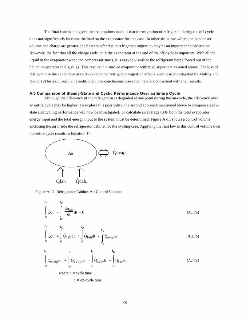
99

The final conclusion given the assumptions made is that the migration of refrigerant during the off-cycle

does not significantly increase the load on the evaporator for this case. In other situations where the condenser

volume and charge are greater, the heat transfer due to refrigerant migration may be an important consideration.

However, the fact that all the charge ends up in the evaporator at the end of the off-cycle is important. With all the

liquid in the evaporator when the compressor starts, it is easy to visualize the refrigerant being forced out of the

helical evaporator in big slugs. This results in a starved evaporator with high superheat as noted above. The loss of

refrigerant in the evaporator at start-up and other refrigerant migration effects were also investigated by Mulroy and

Didion [9] for a split-unit air conditioner. The conclusions presented here are consistent with their results.

A.5 Comparison of Steady-State and Cyclic Performance Over an Entire Cycle Although the efficiency of the refrigerator is degraded at one point during the on-cycle, the efficiency over

an entire cycle may be higher. To explore this possibility, the second approach mentioned above to compare steady-

state and cycling performance will now be investigated. To calculate an average COP both the total evaporator

energy input and the total energy input to the system must be determined. Figure A-11 shows a control volume

enclosing the air inside the refrigerator cabinet for the cycling case. Applying the first law to this control volume over

the entire cycle results in Equation 17.

Qevap..

Air

Qfan Qcab...

Figure A-11. Refrigerator Cabinet Air Control Volume

⌡⌠

o

tc

Q.dt = ⌡

⌠

o

tc

duair

dt dt = 0 (A.17a)

⌡⌠

o

tc

Q.dt = ⌡⌠

o

tc

Q.cabdt + ⌡⌠

o

to

Q.fandt - ∫

ct

o

dtevapQ& (A.17b)

⌡⌠

o

to

Q.evapdt + ⌡⌠

to

tc

Q.evapdt = ⌡⌠

o

tc

Q.cabdt + ⌡⌠

o

to

Q.fandt (A.17c)

where tc = cycle time

to = on-cycle time

100

Equation 17c states that the energy removed by the evaporator during the on-cycle plus that removed

during the off-cycle must equal the energy transferred through the refrigerator cabinet plus the evaporator fan energy

input. Note that the evaporator can absorb energy from the cabinet during the off-cycle after all the refrigerant has

migrated from the condenser. Further, the evaporator fan only runs during the on-cycle. Unfortunately Equation 17c

can not be solved explicitly because the energy input into the evaporator during the off cycle and the cabinet load

are unknown. The cabinet load is not known because of the uncertainty introduced by the door heater. The only

known terms are the energy input to the evaporator during the on cycle and the energy input to the evaporator fan.

However upper and lower bounds can be placed on the total energy input to the evaporator, which is the

left side of Equation 17c, during a cycle. The lower bound occurs for the case where the energy input to the

evaporator during the off cycle is zero. The upper bound occurs when all the refrigerant in the evaporator boils off

during the off cycle.

0

50

100

150

200

250

0

Pow

er a

nd L

oad

(W)

CO

P

0.2

0.4

0.6

0.8

1

0 20 40 60 80 100 120 140Time (min.)

Evaporator LoadCOPSystem Power

Figure A-12. Cycling & Steady-State Evaporator Load

Figure A-12 shows the evaporator load for the on-cycle based on an air side energy balance. Integrating

under this curve yields an average on-cycle evaporator load of 148 W. Multiplying this by the on-cycle time results

in the energy removed by the evaporator during the on-cycle or 223.5 kJ. Therefore the lower bound on the energy

input to the evaporator is 223.5 kJ. The upper bound is easily calculated by multiplying the mass of refrigerant that

boils off by the enthalpy of vaporization of the refrigerant and adding this to the lower bound. If the evaporator is

assumed to contain the entire 7 oz. charge and all the charge boils off during the off cycle at 5°F, then the maximum

energy input to the evaporator during the off cycle is 28.5 kJ. Therefore, the maximum energy input to the evaporator

over an entire cycle is 252 kJ.

The last piece of information needed to calculate an average cycling COP is an average system power

requirement. The variation in the refrigerator power requirement is shown in Figure A-13. The refrigerator power

includes the compressor, the evaporator fan, the condenser fan and the small amount of power drawn by the

controls. The average power for the three on-cycles shown is 188 W. Multiplying this by the on-cycle time of 25.1

minutes yields the energy required over the entire cycle or 283.1 kJ.

101

0

50

100

150

200

250

0

Ref

riger

ator

Sys

tem

Pow

er

20 40 60 80 100 120 140Time (min.)

Cycling Steady State

Figure A-13. System Power for Cyclic & Steady-State Operation

By dividing the minimum and maximum energy inputs to the evaporator by the energy input to the system

over an entire cycle, a minimum and maximu m COP can be determined. Table A.2 summarizes these results. The

average cycling performance is at best 2% lower than the steady state performance and at worst 13%. It again

appears that cycling degrades the performance of the system as for the "snapshot" comparison.

Table A.2. Steady-State and Average Cyclic Performance

Case Steady-State Cycling

Cycle Time (min.) 48.5 48.5 On-Cycle (min.) 48.5 25.1 Off-Cycle (min.) 0.0 23.4 Ambient Temperature (°F) 89.8 89.6 Average Fresh Food Temperature (°F) 41.6 40.1 Average Freezer Temperature (°F) 3.4 4.6 Refrigerant Charge (oz.) 7.0 7.0 Evaporator Load (kJ) 497.7 223.5 to 252 System Energy Input (kJ) 544.2 283.1 Average COP 0.91 0.79 to 0.89

A.6 Conclusions The most important result from this analysis is the fact that refrigerant dynamics have an impact on

performance. Migration of refrigerant between the components of the system results in significant decreases in

efficiency. This means a model to calculate cycling performance must include time dependent charge inventory terms.

Further, it appears that the thermal mass of the compressor must also be considered. A quasi-steady approximation

for the compressor will work. Lastly, the additional heat input to the cabinet due to refrigerant migration appears to be

small for this refrigerator given the assumptions made.

102

References [1] Murphy, W.E., and V.W. Goldschmidt. 1979. "The degradation coefficient of a field-tested self-contained 3-ton

air conditioner." ASHRAE Transactions, Vol. 85, Part 2, pp. 396 to 405.

[2] Goldschmidt, V.W., G.H. Hart, and R. C. Reiner. 1980. "A note on the transient performance and degradation coefficient of a field tested heat pump - cooling and heating mode." ASHRAE Transactions, Vol. 86, Part 2, pp. 368 to 375.

[3] Murphy, W.E., and V.W. Goldschmidt. 1984. "Transient response of air conditioners-a qualitative interpretation through a sample case." ASHRAE Transactions, Vol. 90, Part 1B, pp. 997-1008

[4] Katipamula, S. and D.L. O'Neal. 1991. "Performance degradation during on-off cycling of single-speed heat pumps operating in the cooling mode: experimental results." ASHRAE Transactions, Vol. 97, Part 2, In print.

[5] Department of Energy. 1979. "Test procedures for central air conditioners, including heat pumps." Federal Register, Vol. 44, No. 249, pp. 76700 to 76723.

[6] Department of Energy. 1989. "Uniform test method for measuring the energy consumption of central air-conditioners." Code of Federal Regulations, Part 430, Subpart B, Appendix M, pp. 101 to 126, January 1.

[7] Rohsenow, W.M., "Boiling" in W.M. Rohsenow et al., Eds., Handbook of Heat Transfer Fundamentals , Chapter 12, McGraw-Hill, New York, 1985.

[8] American Society of Heating, Refrigerating and Air-Conditioning Engineers, Inc., Fundamentals Handbook, p. 4.2, ASHRAE, Atlanta, 1989.

[9] Mulroy, W.J. and D.A. Didion. 1985. "Refrigerant migration in a split-unit air conditioner." ASHRAE Transactions, Vol. 91, Part 1A, pp. 193 to 206.

103

Appendix B: Reverse Heat Leak Tests

As part of the parameter estimation effort, the energy transferred through the refrigerator cabinet or cabinet

load may need to be known. The cabinet load can be calculated from Equation 1.

Q. cab = UAfreezer(Tamb - Tfrez) + UAfood(Tamb - Tfood) (B.1)

where UAfreezer = freezer compartment heat transfer coefficient (W/°F)

UAfood = fresh-food compartment heat transfer coefficient (W/°F)

Tamb = chamber temperature (°F)

Tfrez = freezer compartment temperature (°F)

Tfood = fresh-food comp artment temperature (°F)

The freezer compartment, fresh-food compartment and ambient temperatures can be measured directly. The cabinet

over-all heat transfer coefficients or UA values must be determined independently.

These values were found experimentally by performing a reverse heat leak test on the refrigerator cabinet.

The test involves heating both the fresh-food and freezer compartments above ambient conditions with auxiliary

heaters ( see Instrumentation Chapter ) while the refrigerator is turned off. The temperatures in both compartments

were made equal to prevent heat transfer between compartments. Further, the air passages between the

compartments were taped shut. Since the temperature inside the refrigerator is higher than the ambient temperature,

heat is transferred to the environment in the reverse direction it would normally have when the refrigerator is

operating. Once steady-state conditions have been reached, the heat transfer through the cabinet is equal to the

power input to the auxiliary heaters. By dividing the measured powers by the temperature difference between the

internal cabinet temperature and ambient, a UA value can be determined for each compartment.

The power input to the heaters was measured over a range of temperature differences. Figure B-1 shows the

data points taken. The actual temperatures and powers measured are also summarized in Table B.1. The slope of the

lines in Figure B-1 equal the UA values for the freezer and fresh-food compartments. The UA value for the freezer is

0.49 W/°F ± 0.11 W/°F and the UA for the fresh-food compartment is 1.04 W/°F ± 0.11 W/°F.

0.0

10.0

20.0

30.0

40.0

50.0

60.0

70.0

Pow

er In

put (

W)

UAfreezer = 0.49 W/°FUAfood = 1.04 W/°F

80.0

0.0

10.0

20.0

30.0

40.0

50.0

60.0

70.0

80.0

0 10 20 30 40 50 60Temperature Difference (°F)

Freezer CompartmentFresh-Food Compartment

Figure B-1. Reverse Heat Leak Test Results

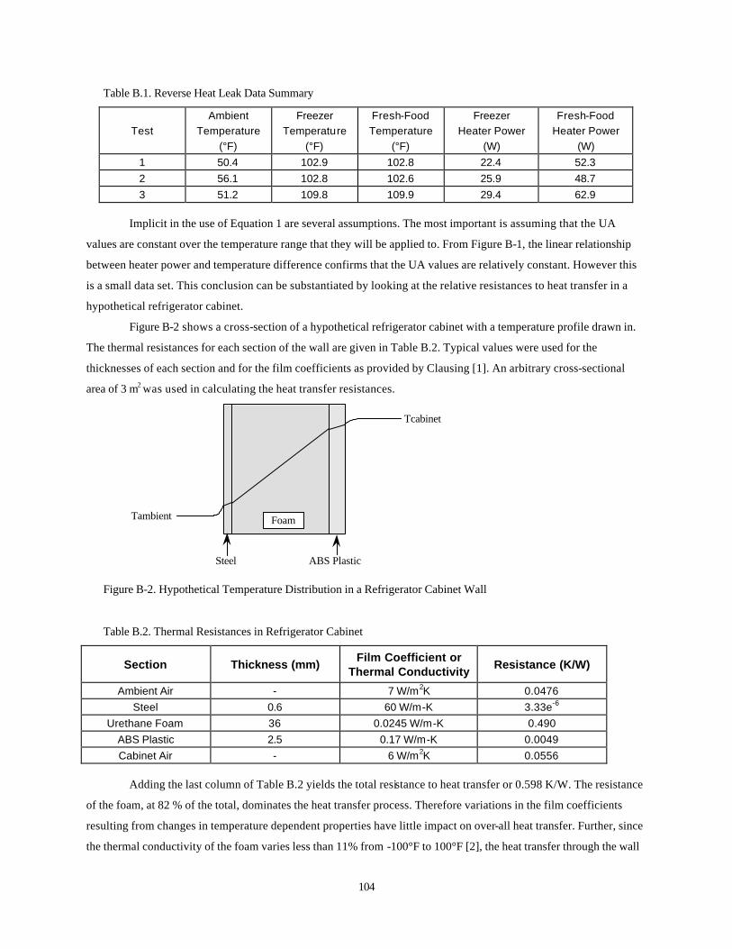
104

Table B.1. Reverse Heat Leak Data Summary

Test

Ambient Temperature

(°F)

Freezer Temperature

(°F)

Fresh-Food Temperature

(°F)

Freezer Heater Power

(W)

Fresh-Food Heater Power

(W) 1 50.4 102.9 102.8 22.4 52.3 2 56.1 102.8 102.6 25.9 48.7 3 51.2 109.8 109.9 29.4 62.9

Implicit in the use of Equation 1 are several assumptions. The most important is assuming that the UA

values are constant over the temperature range that they will be applied to. From Figure B-1, the linear relationship

between heater power and temperature difference confirms that the UA values are relatively constant. However this

is a small data set. This conclusion can be substantiated by looking at the relative resistances to heat transfer in a

hypothetical refrigerator cabinet.

Figure B-2 shows a cross-section of a hypothetical refrigerator cabinet with a temperature profile drawn in.

The thermal resistances for each section of the wall are given in Table B.2. Typical values were used for the

thicknesses of each section and for the film coefficients as provided by Clausing [1]. An arbitrary cross-sectional

area of 3 m2 was used in calculating the heat transfer resistances.

Foam

Steel ABS Plastic

Tcabinet

Tambient

Figure B-2. Hypothetical Temperature Distribution in a Refrigerator Cabinet Wall

Table B.2. Thermal Resistances in Refrigerator Cabinet

Section Thickness (mm) Film Coefficient or

Thermal Conductivity Resistance (K/W)

Ambient Air - 7 W/m2K 0.0476 Steel 0.6 60 W/m-K 3.33e-6

Urethane Foam 36 0.0245 W/m-K 0.490 ABS Plastic 2.5 0.17 W/m-K 0.0049 Cabinet Air - 6 W/m2K 0.0556

Adding the last column of Table B.2 yields the total resistance to heat transfer or 0.598 K/W. The resistance

of the foam, at 82 % of the total, dominates the heat transfer process. Therefore variations in the film coefficients

resulting from changes in temperature dependent properties have little impact on over-all heat transfer. Further, since

the thermal conductivity of the foam varies less than 11% from -100°F to 100°F [2], the heat transfer through the wall

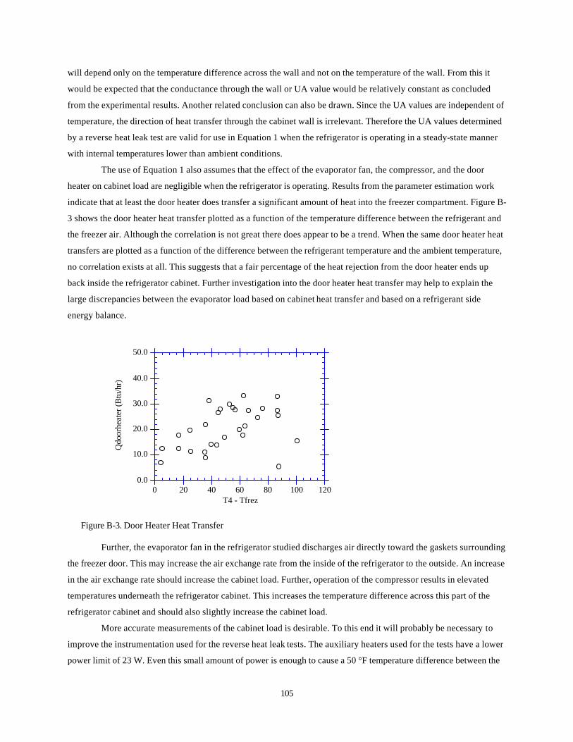
105

will depend only on the temperature difference across the wall and not on the temperature of the wall. From this it

would be expected that the conductance through the wall or UA value would be relatively constant as concluded

from the experimental results. Another related conclusion can also be drawn. Since the UA values are independent of

temperature, the direction of heat transfer through the cabinet wall is irrelevant. Therefore the UA values determined

by a reverse heat leak test are valid for use in Equation 1 when the refrigerator is operating in a steady-state manner

with internal temperatures lower than ambient conditions.

The use of Equation 1 also assumes that the effect of the evaporator fan, the compressor, and the door

heater on cabinet load are negligible when the refrigerator is operating. Results from the parameter estimation work

indicate that at least the door heater does transfer a significant amount of heat into the freezer compartment. Figure B-

3 shows the door heater heat transfer plotted as a function of the temperature difference between the refrigerant and

the freezer air. Although the correlation is not great there does appear to be a trend. When the same door heater heat

transfers are plotted as a function of the difference between the refrigerant temperature and the ambient temperature,

no correlation exists at all. This suggests that a fair percentage of the heat rejection from the door heater ends up

back inside the refrigerator cabinet. Further investigation into the door heater heat transfer may help to explain the

large discrepancies between the evaporator load based on cabinet heat transfer and based on a refrigerant side

energy balance.

0.0

10.0

20.0

30.0

40.0

50.0

0

Qdo

orhe

ater

(Btu

/hr)

20 40 60 80 100 120T4 - Tfrez

Figure B-3. Door Heater Heat Transfer

Further, the evaporator fan in the refrigerator studied discharges air directly toward the gaskets surrounding

the freezer door. This may increase the air exchange rate from the inside of the refrigerator to the outside. An increase

in the air exchange rate should increase the cabinet load. Further, operation of the compressor results in elevated

temperatures underneath the refrigerator cabinet. This increases the temperature difference across this part of the

refrigerator cabinet and should also slightly increase the cabinet load.

More accurate measurements of the cabinet load is desirable. To this end it will probably be necessary to

improve the instrumentation used for the reverse heat leak tests. The auxiliary heaters used for the tests have a lower

power limit of 23 W. Even this small amount of power is enough to cause a 50 °F temperature difference between the

106

freezer compartment and ambient conditions as shown in Figure B-1. A heater system that can deliver less than 23 W

would be desirable. This change will also require watt transducers that can accurately read the small power inputs

required.

One possibility for improving the accuracy of the measurements is to switch to a direct current system. The

voltage and current input to the heater elements could be measured accurately even at these lower power levels. The

system should still include some sort of fan to distribute the air in both compartments to help prevent temperature

gradients within the cabinet. Note that the presence of a fan restricts the maximum internal cabinet temperature that

can be tested. The temperature rating of the insulation of the motor windings should be considered when performing

tests. Typically the insulation on the windings can tolerate temperatures up to 105°F.

References [1] Personal communication., Dr. A. E. Clausing., Associate Head, Department of Mechanical Engineering,

University of Illinois, 1206 West Green Street, Urbana, IL. 61801.

[2] American Society of Heating, Refrigerating and Air-Conditioning Engineers, Inc., Fundamentals Handbook, pg 22.17, ASHRAE, Atlanta, 1989.

107

Appendix C: Refrigerator Charge Tests

As part of the experimental program a series of charge tests was performed on the refrigerator as received

from the manufacturer and after the pressure transducers and the immersion thermocouples were installed (See

Instrumentation Chapter). The purpose of these tests is twofold. First the optimum charge for steady-state operation

based on efficiency for the refrigerator can be determined. Further by ensuring that the refrigerator always runs with

the optimum charge, errors resulting from changes in the amount of charge can be eliminated from a given data set.

Second the effect of the instrumentation on refrigerator performance can be determined.

The procedure for the charge tests is relatively simple. The charge in the refrigerator is varied in roughly one

ounce increments. At each charge level, the internal cabinet temperatures are set as close to 41.4°F in the fresh-food

compartment and 3.3°F in the freezer compartment as possible. For some cases the capacity of the system was

sufficiently reduced such that these compartment temperatures could not be reached. This does not, however, affect

the results. The ambient temperature is also kept constant. Once steady-state conditions are reached, system data is

collected for at least an hour. After each test point, the refrigerant charge in the system is removed.

The charge in the system is removed through the process tube on the compressor with a vacuum pump. The

pump should be allowed to run for a minimum of 2 hours. Shorter evacuation times do not remove all the refrigerant

dissolved in the comp ressor oil. After evacuation, the system is charged from a refrigerant tank that is placed on top

of a digital scale. The scale allows the mass of charge metered into the system to be controlled to within ±0.035

ounce. After being recharged with a different amount of refrigerant, the test is repeated using the same procedure

outlined above.

In all, 4 sets of charge tests were performed. Two tests were run on the refrigerator as received from the

manufacturer: one at 70°F and one at 90°F ambient. For these two tests, only power inputs, air temperatures and

surface temperatures on the heat exchangers were measured. The instrumentation for the first two tests did not

penetrate the refrigerant piping and should not affect the performance of refrigerator. After the pressure transducers

and immersion thermocouples were installed, two more tests were run at the same ambient conditions as for the first

two tests. The experimental results are summarized in Table C.1. The evaporator load is the sum of the power inputs

to the auxiliary heaters ( see Instrumentation Chapter ), the evaporator fan and the cabinet load. The cabinet load was

determined from Equation 1 given in Appendix B. COP or coefficient of performance is the ratio of the evaporator load

to the system power requirement.

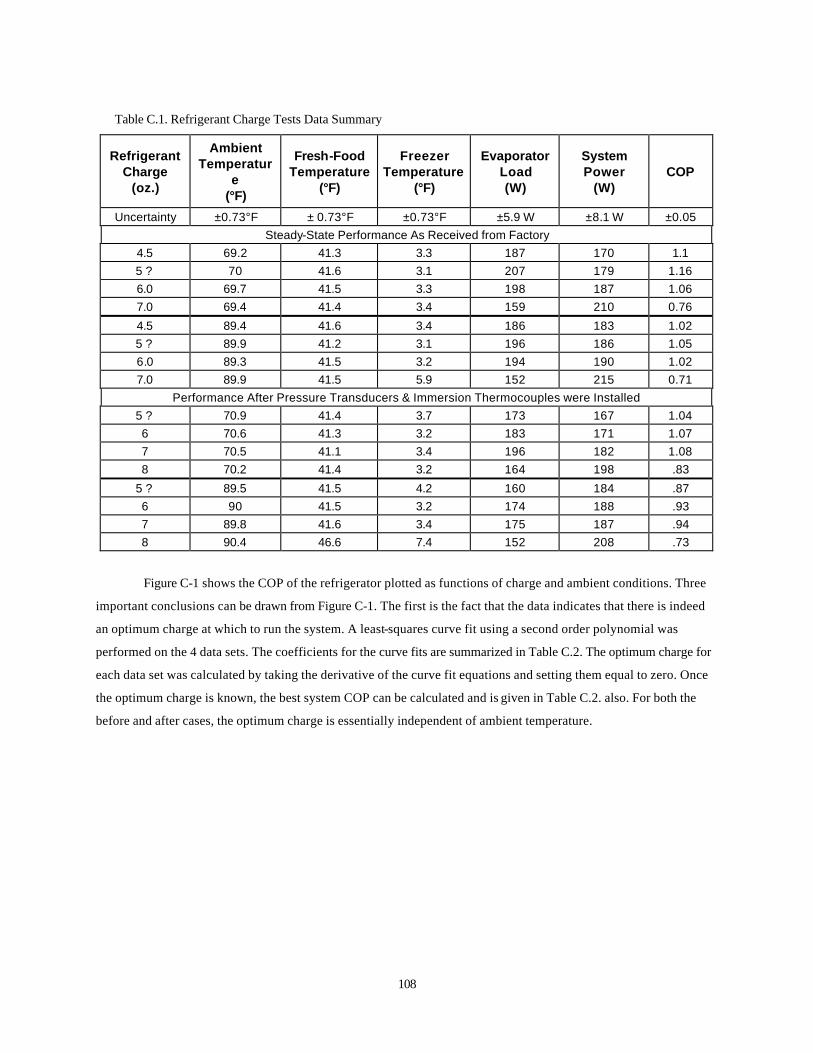
108

Table C.1. Refrigerant Charge Tests Data Summary

Refrigerant Charge

(oz.)

Ambient Temperatur

e (°F)

Fresh-Food Temperature

(°F)

Freezer Temperature

(°F)

Evaporator Load (W)

System Power

(W) COP

Uncertainty ±0.73°F ± 0.73°F ±0.73°F ±5.9 W ±8.1 W ±0.05 Steady-State Performance As Received from Factory

4.5 69.2 41.3 3.3 187 170 1.1 5 ? 70 41.6 3.1 207 179 1.16 6.0 69.7 41.5 3.3 198 187 1.06 7.0 69.4 41.4 3.4 159 210 0.76

4.5 89.4 41.6 3.4 186 183 1.02 5 ? 89.9 41.2 3.1 196 186 1.05 6.0 89.3 41.5 3.2 194 190 1.02 7.0 89.9 41.5 5.9 152 215 0.71

Performance After Pressure Transducers & Immersion Thermocouples were Installed 5 ? 70.9 41.4 3.7 173 167 1.04 6 70.6 41.3 3.2 183 171 1.07 7 70.5 41.1 3.4 196 182 1.08 8 70.2 41.4 3.2 164 198 .83

5 ? 89.5 41.5 4.2 160 184 .87 6 90 41.5 3.2 174 188 .93 7 89.8 41.6 3.4 175 187 .94 8 90.4 46.6 7.4 152 208 .73

Figure C-1 shows the COP of the refrigerator plotted as functions of charge and ambient conditions. Three

important conclusions can be drawn from Figure C-1. The first is the fact that the data indicates that there is indeed

an optimum charge at which to run the system. A least-squares curve fit using a second order polynomial was

performed on the 4 data sets. The coefficients for the curve fits are summarized in Table C.2. The optimum charge for

each data set was calculated by taking the derivative of the curve fit equations and setting them equal to zero. Once

the optimum charge is known, the best system COP can be calculated and is given in Table C.2. also. For both the

before and after cases, the optimum charge is essentially independent of ambient temperature.

109

0

0.2

0.4

0.6

0.8

1C

OP

1.2

4 5 6 7 8 9

Factory Performance - 70°F

Refrigerant Charge (oz.)

Factory Performance - 90°FAfter Instrumentation - 70°FAfter Instrumentation - 90°F

Figure C-1. Effect of Charge on Refrigerator Performance - R12

Table C.2. Coefficients for Curve Fits of Charge Data

Test Case A B C Optimum Charge

(oz.) Optimum COP

Before - 70°F -0.11721 1.21431 -2.05876 5.2 1.09 Before - 90°F -0.11532 1.21244 -2.18375 5.3 1.0 After - 70°F -0.09819 1.24228 -2.8896 6.3 1.04 After - 90°F -0.07986 1.02248 -2.39549 6.4 0.88

Curve Fits of the Form COP = A(charge)2 + B(charge) + C

The second important trend shown in Figure C-1 is the shift in the average optimum operating charge from

5.25 oz. to 6.35 oz. The most logical cause for the shift is the extra volume added to the system by the pressure

transducers and the immersion thermocouples. The added volume has no effect on system performance other than

increasing the amount of charge required to bring the refrigerator up to optimum performance.

The third and most important trend shown in Figure C-1 is the decrease in the optimum efficiency of the

system for equivalent ambient conditions. This indicates that the pressure transducers and immersion thermocouples

have an effect on refrigerator performance. One possible explanation for the reduction is an increase in the pressure

drop in the system caused by the instrumentation tees (See Instrumentation Chapter). Increased pressure drop in the

system would increase the pressure difference across the compressor which would reduce the mass flow rate. A

lower mass flow rate results in a lower capacity and a lower efficiency for equivalent operating conditions.

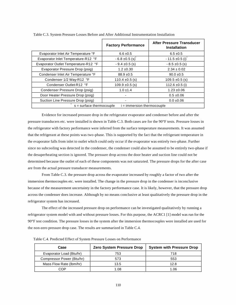
110

Table C.3. System Pressure Losses Before and After Additional Instrumentation Installation

Factory Performance

After Pressure Transducer Installation

Evaporator Inlet Air Temperature °F 6.6 ±0.5 6.5 ±0.5 Evaporator Inlet Temperature-R12 °F - 6.8 ±0.5 (s)* - 11.5 ±0.5 (i)*

Evaporator Outlet Temperature-R12 °F - 9.4 ±0.5 (s) - 8.5 ±0.5 (s) Evaporator Pressure Drop (psig) 1.2 ±0.30 2.34 ± 0.02

Condenser Inlet Air Temperature °F 88.9 ±0.5 90.0 ±0.5 Condenser 1/2 Way-R12 °F 110.4 ±0.5 (s) 109.5 ±0.5 (s) Condenser Outlet-R12 °F 109.9 ±0.5 (s) 112.6 ±0.5 (i)

Condenser Pressure Drop (psig) 1.0 ±1.4 1.23 ±0.06 Door Heater Pressure Drop (psig) - 0.5 ±0.06 Suction Line Pressure Drop (psig) - 0.0 ±0.06

* s = surface thermocouple i = immersion thermocouple

Evidence for increased pressure drop in the refrigerator evaporator and condenser before and after the

pressure transducers etc. were installed is shown in Table C.3. Both cases are for the 90°F tests. Pressure losses in

the refrigerator with factory performance were inferred from the surface temperature measurements. It was assumed

that the refrigerant at these points was two-phase. This is supported by the fact that the refrigerant temperature in

the evaporator falls from inlet to outlet which could only occur if the evaporator was entirely two-phase. Further

since no subcooling was detected in the condenser, the condenser could also be assumed to be entirely two-phase if

the desuperheating section is ignored. The pressure drop across the door heater and suction line could not be

determined because the outlet of each of these components was not saturated. The pressure drops for the after case

are from the actual pressure transducer measurements.

From Table C.3. the pressure drop across the evaporator increased by roughly a factor of two after the

immersion thermocouples etc. were installed. The change in the pressure drop in the condenser is inconclusive

because of the measurement uncertainty in the factory performance case. It is likely, however, that the pressure drop

across the condenser does increase. Although by no means conclusive at least qualitatively the pressure drop in the

refrigerator system has increased.

The effect of the increased pressure drop on performance can be investigated qualitatively by running a

refrigerator system model with and without pressure losses. For this purpose, the ACRC1 [1] model was run for the

90°F test condition. The pressure losses in the system after the immersion thermocouples were installed are used for

the non-zero pressure drop case. The results are summarized in Table C.4.

Table C.4. Predicted Effect of System Pressure Losses on Performance

Case Zero System Pressure Drop System with Pressure Drop

Evaporator Load (Btu/hr) 753 718 Compressor Power (Btu/hr) 573 553

Mass Flow Rate (lbm/hr) 13.5 12.8 COP 1.08 1.06

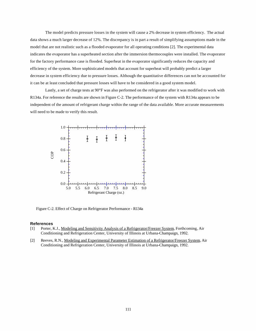
111

The model predicts pressure losses in the system will cause a 2% decrease in system efficiency. The actual

data shows a much larger decrease of 12%. The discrepancy is in part a result of simplifying assumptions made in the

model that are not realistic such as a flooded evaporator for all operating conditions [2]. The experimental data

indicates the evaporator has a superheated section after the immersion thermocouples were installed. The evaporator

for the factory performance case is flooded. Superheat in the evaporator significantly reduces the capacity and

efficiency of the system. More sophisticated models that account for superheat will probably predict a larger

decrease in system efficiency due to pressure losses. Although the quantitative differences can not be accounted for

it can be at least concluded that pressure losses will have to be considered in a good system model.

Lastly, a set of charge tests at 90°F was also performed on the refrigerator after it was modified to work with

R134a. For reference the results are shown in Figure C-2. The performance of the system with R134a appears to be

independent of the amount of refrigerant charge within the range of the data available. More accurate measurements

will need to be made to verify this result.

0.0

0.2

0.4

0.6

0.8

1.0

5.0 5.5 6.0

CO

P

6.5 7.0 7.5 8.0 8.5 9.0Refrigerant Charge (oz.)

Figure C-2. Effect of Charge on Refrigerator Performance - R134a

References [1] Porter, K.J., Modeling and Sensitivity Analysis of a Refrigerator/Freezer System, Forthcoming, Air

Conditioning and Refrigeration Center, University of Illinois at Urbana-Champaign, 1992.

[2] Reeves, R.N., Modeling and Experimental Parameter Estimation of a Refrigerator/Freezer System, Air Conditioning and Refrigeration Center, University of Illinois at Urbana-Champaign, 1992.

112

Appendix D: Experimental Uncertainty Analysis

Temperature Measurement Uncertainty

Data Acquisition Supplier Estimate ±1.3 °F Lab Estimate ±0.73 °F

Uncertainty = (Bias)2 + (Precision error)2

Precision error = 2Sx = 2(0.266 °F) = ± 0.532 °F

Uncertainty = (0.5 °F)2 + (0.532 °F)2 = ±0.73 °F

Pressure Transducer Uncertainties

Pressure Transducer

Type

Transducer Accuracy

Load Resistor

Atmospheric Pressure Variation

Precision Error

Total Uncertainty

0-100 psi gage ±0.13 psi - ±0.4 psi ±0.38 psi ±0.57 psi 0-250 psi gage ±0.325 psi - ±0.4 psi ±0.66 psi ±0.84 psi

0-10 psi differential ±0.015 psi ±0.015 psi - ±0.14 psi ±0.14 psi 0-25 psi

differential ±0.05 psi ±0.038 psi - ±0.09 psi ±0.11 psi

Sample calculation 0-10 psi differential pressure transducer:

(Transducer output = 4 to 20 mA through 25 Ω resistor to get 0.1 V to 0.5 V output)

Transducer accuracy = (instrument accuracy)(full scale)

= (0.15 %)(10 psi) = ±0.015 psi

Load resistor error = 10 psi0.4 V [(variation in voltage output due to temperature)]

= 10 psi0.4 V [(30 ppm/°F)(40 °F)(25 Ω)(20 mA)(1/1000)] = ±0.015 psi

Precision error = 2(0.07 psi) = ±0.14 psi

Uncertainty = (0.015 psi)2 + (0.015 psi)2 + (0.14 psi)2 = ±0.14 psi

Sample calculation 0-100 psig pressure transducer

Transducer output = 0.1 V to 5.1 V

Transducer accuracy = (instrument accuracy)(full)(scale)

= (0.13 %)(100 psig) = ±0.13 psig

Atmospheric pressure variation from lab data = ±0.4 psi

Precision error = 2(0.19 psi) = ±0.38 psi

Uncertainty = (0.13 psi)2 + (0.4 psi)2 + (0.38 psi)2 = ±0.57 psi

113

Uncertainty in Measured Pressures

Pressure (psi) Uncertainty

Evaporator Inlet ±0.59 psi Evaporator Outlet ±0.57 psi

Compressor Suction Inlet ±0.58 psi Condenser Inlet ±0.85 psi

Condenser Outlet ±0.84 psi Capillary Tube Inlet ±0.85 psi

Sample calculation for capillary tube inlet:

Pcapinlet = Pcondenser out - ∆Pdoor heater

Uncertainty = (uncertainty in Pcondenser)2 + (uncertainty in ∆P)2

Uncertainty = (0.84 psi)2+(0.11 psi)2 = ±0.85 psi

Watt Transducer Uncertainty

Watt Transducer Transducer Uncertainty

Load Resistor

Voltage Ripple

Precision Error

Total Uncertainty

System ±7.5 W ±2.3 W - ±2.2 W ±8.1 W Compressor ±2.5 W ±0.8 W - ±2.1 W ±3.4 W

Evaporator Fan ±0.5 W - - ±0.21 W ±0.5 W Freezer Heater ±1.1 W ±0.6 W ±2.5 W - ±2.8 W

Fresh Food Heater ±1.1 W ±0.6 W ±2.5 W - ±2.8 W Sample calculation, system power:

Transducer output: 4 - 20 mA through 25 Ω resistor to get 0.1 V to 0.5 V output

Transducer uncertainty = (transducer accuracy)(full scale)

= (0.5 %)(1500 W) = ±7.5 W

Load resistor = 1500 W

0.4 V [variation in voltage due to temperature flucuations]

= 1500 W

0.4 V [(30 ppm/°F)(40 °F)(25 Ω)(20 mA)(1/1000)] = ±2.3 W

Precision error = 2(1.1 W) = ±2.2 W

Uncertainty = (7.5 W)2 + (2.3 W)2 + (2.2 W)2 = ±8.1 W

Sample calculation, freezer heater power:

Transducer output - 0 to 1 ma through 10 kΩ resistor to get 0 to 10 V output

Transducer uncertainty = (transducer accuracy)(full scale)

= (0.21 %)(500 W) = ±1.05 W

114

Load resistor = 500 W10 V [variation in voltage due to temperature flucuations]

= 500 W10 V [(30 ppm/°F)(40 °F)(10 kΩ)(1 mA)] = ±0.6 W

Voltage ripple = 500 W10 V [variation in voltage due to RC circuit ]

Voltage ripple = 500 W10 V (0.05 V) = ± 2.5 W

Uncertainty = (1.05 W)2 + (0.6 W)2 + (2.5 W)2 = ±2.8 W

Uncertainty in Enthalpy Calculations

Location δhδT

Uncertainty in Temperature

δhδP

Uncertainty in

Pressure Total

Uncertainty

Evaporator Outlet - R12

0.14 Btu/lbm°F ±0.73 °F -0.0552 Btu/lbm*psi

±0.57 psi ±0.11 Btu/lbm

Compressor Discharge - R12

0.17 Btu/lbm°F @ 140 psia, 160°F

±0.73 °F

-0.0335 Btu/lbm*psi

±0.85 psi

±0.13 Btu/lbm

Condenser Outlet - R12

0.24 Btu/lbm°F ±0.73 °F 0.131 Btu/lbm*psi

±0.84 psi ±0.21 Btu/lbm

Evaporator Outlet - R134a

0.19 Btu/lbm°F @ 10.4 psia, 20 °F

±0.73 °F

-0.089 Btu/lbm*psi

±0.0 psi

±0.14 Btu/lbm

Compressor Discharge -

R134a

0.251 Btu/lbm°F @ 132 psia, 150 °F

±0.73 °F

-0.050 Btu/lbm*psi

±0.85 psi

±0.19 Btu/lbm

Condenser Outlet - R134a

0.35 Btu/lbm°F @ 132 psia, x=0.0

±0.73 °F 0.113 Btu/lbm*psi

±0.84 psi ±0.27 Btu/lbm

Sample calculation, evaporator outlet:

δhδT

= ∆h∆T

= 80.767 - 79.345Btu/lbm

20-10°F = 0.14 Btu/lbm°F @ P=20psia,T=10°F,20°F

δhδP

= ∆h∆P

= 81.043 - 80.767Btu/lbm

15-20psia = -0.0552 Btu/lbm*psi @T=20°F,P=15psia,20psia

Total uncertainty =

22

)P(wTh)T(w

Th

δδ+

δδ

= (0.14*0.73)2 + (-0.0552*0.57)2 = ±0.11 Btu/lbm

Sample calculation, condenser outlet (assume saturated liquid)

δhδT

= Cp(@100°F) = 0.24 Btu/lbm°F

δhδP

= ∆h∆P

= 31.583-31.1Btu/lbm135.56-131.86psia = 0.131 Btu/lbm*psia

115

Total uncertainty = (0.24*0.73)2 + (0.131*0.84)2 = ±0.21 Btu/lbm

Refrigerant Mass Flow Rate Uncertainties

Source Uncertainty

Compressor Map ±5.0 % Turbine Flow Meter ± 2.9%

Turbine flow meter calculation:

Transducer accuracy = ±0.25%

Calbration error = ±1%

Mean deviation from curve fit = ±2.7%

Total uncertainty = (0.0025 )2 + (0.01 )2 + (0.027)2 = ±0.029

Condenser Volumetric Flow Rate Uncertainty

V. c =

1ρCp60∆T

3.413 (P.system - P

.efan) + m

. (h10 - h3)

nominal values: ρ = 0.072 lbm/ft3, Cp = 0.24 Btu/lbm°F, ∆T = 9.3 °F

Psystem = 160 W, Pefan = 12.5 W, m. = 7.5 lbm/hr

h10 = 116 Btu/lbm, h3 = 35 Btu/lbm

w(ρ) = δρδΤ

w(T) = (1.33e-4 lbm/ft3°F)(±0.73 °F) = ±9.7e-5 lbm/ft3

w(V. c (ρ)) =

δV.c

δρ w(ρ) = (-1584.4)(±9.7e-5) = ±0.154 ft3/min

w(Cp) = δCpδΤ

w(T) = (2.24e-5 Btu/lbm°F2)(±0.73 °F) = ±1.64e-5 Btu/lbm°F

w(V. c (Cp)) =

δV.c

δCp w(CP) = (-475.3)(±1.64e-5) = ±7.79e-3 ft3/min

w(V. c (∆T)) =

δV.c

δ∆T w(∆T) = (-12.3)(±1.03°F) = ±12.7 ft3/min

w(V. c (P

. system)) =

δV.c

δP.system

) w(P. system)) = (0.354)(±8.1 W) = ±2.87 ft3/min

116

w(V. c (P

. efan)) =

δV.c

δP.efan

) w(P. efan)) = (-0.354)(±0.5 W) = ±0.177 ft3/min

w(V. c (m

. )) =

δV.c

δm. w(m

. ) = (8.401)(2.9%)(7.5 lbm/hr) = ±1.8 ft3/min

w(V. c (h10)) =

δV.c

δh10 w(h10) = (0.778)(±0.14 Btu/lbm) = ±0.11 ft3/min

w(V. c (h3)) =

δV.c

δh3 w(h3) = (-0.778)(±0.19 Btu/lbm) = ±0.15 ft3/min

w(V. c) = ∑

i=1

8

[ ](wi2) = ±13.1 ft3/min

w(ρCp60∆T) = (0.072 lbm/ft3)(0.24 Btu/lbm°F)(60)(9.3 °F)

±9.7e-5 lbm/ft3

0.072 lbm/ft32 +

±1.64e-5 Btu/lbm°F

0.24 Btu/lbm°F2 +

±1.03 °F

9.3 °F2

w(ρCp60∆T) = ±1.07 Btu*min/ft3hr

w((3.413 (P. system - P

. efan)) = 3.413 (±8.1 W)2 + (±0.5 W)2 = ±27.7 Btu/hr

w(m. (h10 - h3) ) = (7.5 lbm/hr)(81 Btu/lbm)

±0.218 lbm/hr

7.5 lbm/hr2 +

±0.24 Btu/lbm

81 Btu/lbm2

w(m. (h10 - h3) ) = ± 17.8 Btu/hr

w((3.413 (P. system - P

. efan) + m

. (h10 - h3) )

= (±27.7 W)2 + (±17.8 W)2 = ±32.9 Btu/hr

Condenser Heat Transfer & Conductance Uncertainties R134a case

nominal values: Q. c = 705.2 Btu/hr, Q

. desup = 108.4 Btu/hr, Q

. 2ph = 565.2 Btu/hr,

Q. sub = 31.5 Btu/hr, h1 = 127.1 Btu/lbm, h1sat = 113 Btu/lbm

h2 = 39.5 Btu/lbm, h3 = 35.4 Btu/lbm, T1 = 143.9 °F

cmin = 1.925 Btu/hr°F, cminsub = 2.623 Btu/hr°F, T2 = 87.7 °F

cacond = 122.47 Btu/hr°F, Tconairin = 68.9°F, m. = 7.69 lbm/hr

117

Udesup = 4.79257,U2ph = 29.6175,Usub = 11.1398 Btu/ft2hr°F

adesup = 0.658 ft2, a2ph = 1.185 ft2, asub = 0.247 ft2

Tconmid1 = 69.2°F, Tconmid2 = 73.8°F

Q. c = m

. (h1 - h3) = m

. ∆h

Q. desup = m

. (h1 - h1sat) = m

. ∆h

Q. 2ph = m

. (h1sat - h2) = m

. ∆h

Q. sub = m

. (h2 - h3) = m

. ∆h

w(Q. c) = (7.69 lbm/hr)(91.7 Btu/lbm)

±0.223 lbm/hr

7.69 lbm/hr2 +

±0.33 Btu/lbm

91.7 Btu/lbm2

= ± 20.6 Btu/hr

w(Q. desup) = (7.69 lbm/hr)(14.1 Btu/lbm)

±0.223 lbm/hr

7.69 lbm/hr2 +

±0.27 Btu/lbm

14.1 Btu/lbm2

= ± 3.8 Btu/hr

w(Q. 2ph) = (7.69 lbm/hr)(73.5 Btu/lbm)

±0.223 lbm/hr

7.69 lbm/hr2 +

±0.38 Btu/lbm

73.5 Btu/lbm2

= ± 16.6 Btu/hr

w(Q. sub) = (7.69 lbm/hr)(4.1 Btu/lbm)

±0.223 lbm/hr

7.69 lbm/hr2 +

±0.33 Btu/lbm

4.1 Btu/lbm2

= ±2.7 Btu/hr

w(Tconmid1) = w(Q.sub

cacond + Tconairin)

w(Q.sub

cacond ) = 31.5 Btu/hr

122.47 Btu/hr°F

±2.7 Btu/hr

31.5 Btu/hr2 +

±13.6 Btu/hr°F

122.47 Btu/hr°F2 = ±0.036 °F

w(Tconairin) = ±0.73°F

w(Tconmid1) = ±0.73°F

w(Tconmid2) = w(Q.2ph

cacond + Tconmid1)

w(Q.2ph

cacond ) = 565.2 Btu/hr

122.47 Btu/hr°F

±16.6 Btu/hr

565.2 Btu/hr2 +

±13.6 Btu/hr°F

122.47 Btu/hr°F2 = ±0.53 °F

w(Tconmid2) = ±0.90°F

118

Desuperheating section

m. (h1-h1sat) = m

. ∆h =

1 - e

-Udesup adesup

cmin (1-cmin/cacond)

1 - (cmin/cacond) e

-Udesup adesup

cmin (1-cmin/cacond)

cmin (T1 - Tconmid2)

w(Udesup(m. )) =

δUdesup

δm. w(m

. ) = (1.61)(±2.9%)(7.69 lbm/hr) = ±0.36 Btu/hr°F*ft2

w(Udesup(∆h)) = δUdesup

δ∆h w(∆h) = (0.876)(±0.269 Btu/lbm) = ±0.24 Btu/hr°F*ft2

w(Udesup(cmin)) = δUdesup

δcmin w(cmin) ˜ (-3.653)(±2.9%)(7.69 lbm/hr)(0.25 Bti/lbm°F)

= ±0.20 Btu/hr°F*ft2

w(Udesup(cacond)) = δUdesupδcacond

w(cacond)

˜ (-3.12e-4)(0.072 lbm/ft3)(0.24 Btu/lbm°F)(60)(±13.1 ft3min) = ±4.24e-3 Btu/hr°F*ft2

w(Udesup(T1)) = δUdesup

δT1 w(T1) = (-1.63e-1)(±0.73°F) = ±0.12 Btu/hr°F*ft2

w(Udesup(Tconmid2)) = δUdesup

δTconmid2 w(Tconmid2) = (1.78e-1)(±0.9°F)

= ±0.16 Btu/hr°F*ft2

w(Udesup) = ∑i=1

6

[ ](wi2) = ±0.52 Btu/hr°F*ft2

Two-phase section

m. (h1sat-h2) = m

. ∆h = 1 - e

(-U2ph a2ph/cacond) cacond (T2 - Tconmid1)

w(U2ph(m. )) =

δU2ph

δm. w(m

. ) = (4.467)(±2.9%)(7.69 lbm/hr) = ±1.0 Btu/hr°F*ft2

w(U2ph(∆h)) = δU2ph

δ∆h w(∆h) = (0.467)(±0.38 Btu/lbm) = ±0.18 Btu/hr°F*ft2

w(U2ph(cacond)) = δU2ph

δcacond w(cacond)

119

˜ (-0.038)(0.072 lbm/ft3)(0.24 Btu/lbm°F)(60)(±13.1 ft3min) = ±0.52 Btu/hr°F*ft2

w(U2ph(T2)) = δU2ph

δT2 w(T2) = (-1.737)(±0.73°F) = ±1.27 Btu/hr°F*ft2

w(U2ph(Tconmid1)) = δU2ph

δTconmid1 w(Tconmid1) = (1.935)(±0.73°F)

= ±1.4 Btu/hr°F*ft2

w(U2ph) = ∑i=1

5

[ ](wi2) = ±2.2 Btu/hr°F*ft2

Subcooled section

m. (h2-h3) = m

. ∆h =

1 - e

-Usub asub

cminsub (1-cminsub/cacond)

1 - (cminsub/cacond) e

-Usub asub

cminsub (1-cminsub/cacond)

cminsub (T2 - Tconairin)

w(Usub(m. )) =

δUsub

δm. w(m

. ) = (2.584)(±2.9%)(7.69 lbm/hr) = ±0.58 Btu/hr°F*ft2

w(Usub(∆h)) = δUsub

δ∆h w(∆h) = (4.847)(±0.33 Btu/lbm) = ±1.6 Btu/hr°F*ft2

w(Usub(cmin)) = δUsubδcmin

w(cmin) ˜ (-3.158)(±2.9%)(7.69 lbm/hr)(0.341 Bti/lbm°F)

= ±0.24 Btu/hr°F*ft2

w(Usub(cacond)) = δUsub

δcacond w(cacond)

˜ (-7.38e-4)(0.072 lbm/ft3)(0.24 Btu/lbm°F)(60)(±13.1 ft3min) = ±0.01 Btu/hr°F*ft2

w(Usub(T2)) = δUsub

δT2 w(T2) = (-9.71e-1)(±0.73°F) = ±0.71 Btu/hr°F*ft2

w(Usub(Tconairin)) = δUsub

δTconairin w(Tconairin) = (1.14)(±0.73°F)

= ±0.83 Btu/hr°F*ft2

w(Usub) = ∑i=1

6

[ ](wi2) = ±2.0 Btu/hr°F*ft2

120

R12 case

nominal values: Q. c = 1103 Btu/hr, Q

. 2ph = 900 Btu/hr, Q

. desup = 202.9 Btu/hr

P. system = 222.3 W, P

. efan = 12.3 W, m

. = 15.41 lbm/hr, h1 = 101.7 Btu/lmb

h2 = 88.54 Btu/lbm, h10 = 91.93 Btu/lbm, T1 = 189.6 °F, T2 = 119.1°F

Tconairin = 89.1°F, Tconmid = 96.7 °F, Tconairout = 98.4°F

Tconfanout = 103.2°F, cmin = 2.86 Btu/hr°F, cacond = 118.1 Btu/hr°F

ρ = 0.071 lbm/ft3, Cp = 0.24 Btu/lbm°F, V. c = 115.8 ft3/min, a2ph = 0.916 ft2

adesup = 1.174 ft2, Udesup = 3.67 Btu/hr°F*ft2, U2ph = 38.28 Btu/hr°F*ft2

Q. c = ρCp60V

. c∆T - 3.413 (P

. system - P

. efan) + m

. (h1 - h10)

w(Q. c(V

. c)) =

δQ.c

δV.c

w(V. c) = (14.416)(±13.1 ft3/min) = ±188.8 Btu/hr

w(Q. c(∆T)) =

δQ.c

δ∆T w(∆T) = (118.394)(±1.03°F) = ±121.9 Btu/hr

w(Q. c(P

. system)) =

δQ.c

δP.system

w(P. system) = (-3.413)(±8.1W) = ±27.6 Btu/hr

w(Q. c(P

. efan)) =

δQ.c

δP.efan

w(P. efan) = (3.413)(±0.5 W) = ±1.7 Btu/hr

w(Q. c(m

. )) =

δQ.c

δm. w(m

. ) = (9.78)(±5.0%)(15.41 lbm/hr) = ±7.5 Btu/hr

w(Q. c(∆h)) =

δQ.c

δ∆h w(∆h) = (15.257)(±0.17 Btu/lbm) = ±2.6 Btu/hr

w(Q. c) = ∑

i=1

6

[ ](wi2) = ±226.5 Btu/hr

Q. desup = m

. (h1 - h2) = m

. ∆h

w(Q. desup) = (15.41 lbm/hr)(13.17 Btu/lbm)

±0.771 lbm/hr

15.41 lbm/hr2 +

±0.18 Btu/lbm

13.17 Btu/lbm2

= ±10.5 Btu/hr

121

w(Tconairout) = w(Q.c

cacond + Tconairin)

w(cacond) ˜ (0.071 lbm/ft3)(0.24 Btu/lbm°F)(60)(±13.1 ft3/min) = ±13.4 Btu/hr°F

w(Q.c

cacond ) = 1103 Btu/hr

118.1 Btu/hr°F

±226.5 Btu/hr

1103 Btu/hr2 +

±13.4 Btu/hr°F

118.1 Btu/hr°F2 = ±2.2 °F

w(Tconairout) = ±2.3°F

w(Tconmid) = w(Tconairout - Q.desup

cacond )

w(Q.desup

cacond ) = 202.9 Btu/hr

118.1 Btu/hr°F

±10.5 Btu/hr

202.9 Btu/hr2 +

±13.4 Btu/hr°F

118.1 Btu/hr°F2 = ±0.21 °F

w(Tconmid) = ±2.3°F

w(Q. 2ph) = w(cacond*(Tconmid - Tconairin))

w(cacond ∆T) = (118.1 Btu/hr°F)(7.6°F)

±2.41°F

7.6°F2 +

±13.4 Btu/hr°F

118.1 Btu/hr°F2

w(Q. 2ph) = ±302.2 Btu/hr

Desuperheating Section

m. (h1-h2) = m

. ∆h =

1 - e

-Udesup adesup

cmin (1-cmin/cacond)

1 - (cmin/cacond) e

-Udesup adesup

cmin (1-cmin/cacond)

cmin (T1 - Tconmid)

w(Udesup(m. )) =

δUdesup

δm. w(m

. ) = (0.563)(±5.0%)(15.41 lbm/hr) = ±0.43 Btu/hr°F*ft2

w(Udesup(∆h)) = δUdesup

δ∆h w(∆h) = (0.659)(±0.18 Btu/lbm) = ±0.12 Btu/hr°F*ft2

w(Udesup(cmin)) = δUdesup

δcmin w(cmin) ˜ (-1.632)(±5.0%)(15.41 lbm/hr)(0.186 Bti/lbm°F)

= ±0.23 Btu/hr°F*ft2

w(Udesup(cacond)) = δUdesupδcacond

w(cacond)

= (-3.64e-4)(±13.4 Btu/hr°F) = ±4.88e-3 Btu/hr°F*ft2

122

w(Udesup(T1)) = δUdesup

δT1 w(T1) = (-8.81e-2)(±0.73°F) = ±0.064 Btu/hr°F*ft2

w(Udesup(Tconmid)) = δUdesup

δTconmid2 w(Tconmid2) = (9.49e-2)(±2.3°F)

= ±0.22 Btu/hr°F*ft2

w(Udesup) = ∑i=1

6

[ ](wi2) = ±0.55 Btu/hr°F*ft2

Two-phase section

Q. 2ph = 1 - e

(-U2ph a2ph/cacond) cacond (T2 - Tconairin)

w(U2ph(Q. 2ph)) =

δU2ph

δQ.2ph

w(Q. 2ph) = (4.91e-2)(±302.2 Btu/hr) = ±14.8 Btu/hr°F*ft2

w(U2ph(cacond)) = δU2ph

δcacond w(cacond)

= (-5.26e-2)(±13.4 Btu/hr°F) = ±0.70 Btu/hr°F*ft2

w(U2ph(T2)) = δU2ph

δT2 w(T2) = (-1.42)(±0.73°F) = ±1.04 Btu/hr°F*ft2

w(U2ph(Tconairin)) = δU2ph

δTconairin w(Tconairin) = (1.54)(±0.73°F)

= ±1.12 Btu/hr°F*ft2

w(U2ph) = ∑i=1

4

[ ](wi2) = ±14.9 Btu/hr°F*ft2

Compressor Shell Heat Transfer Uncertainties

R12 nominal values: Q. comp = 459 Btu/hr, P

. comp = 185.7 W, m

. = 18.4 lbm/hr

h1 = 98.3 Btu/lbm, h10 = 88.8 Btu/lbm, P. evapfan = 12.9 W

P. system = 213.2 W, P

. confan = 14.6 W, Tcompair = 84.1°F

Tconfanout = 84.4°F,ρ = 0.072 lbm/ft3, Cp = 0.24 Btu/lbm°F

T1 = 164.7°F

Q. comp = (3.413 P

. comp ) - m

. (h1 - h10 )

123

w(3.413 P. comp) = ±11.6 Btu/hr

w(m. ∆h) = (18.4 lbm/hr)(9.5 Btu/lbm)

±0.92 lbm/hr

18.4 lbm/hr2 +

±0.17 Btu/lbm

9.5 Btu/lbm2

= ±9.3 Btu/hr

w(Q. comp) = (11.6 Btu/hr)2 + (9.3 Btu/hr)2 ±14.9 Btu/hr

P. confan = P

. system - P

. comp - P

. evapfan

w(P. confan) = (8.1W)2 + (3.4 W)2 + (0.5 W)2 = ±8.8 W

Tcompair = Tconfanout - 3.413 P

.confan

60ρCpV.

w

3.413 P.confan

60ρCpV. =

49.8 Btu/hr120.1 Btu/hr°F

±30.0 Btu/hr

49.8 Btu/hr2 +

±13.6 Btu/hr°F

120.1 Btu/hr°F2

= ±0.25 °F

w(Tcompair) = (0.73°F)2 + (0.25°F)2 = ±0.77°F

w(T1 - Tcompair) = (0.73°F)2 + (0.77°F)2 = ±1.06°F

h_

= Q.comp∆T

w

Q.comp∆T

= 459 Btu/hr

80.6 °F

±14.9 Btu/hr

459 Btu/hr2 +

±1.06 °F

80.6 °F2

w(h_

) = ±0.2 Btu/hr°F

R134a nominal values: Q. comp = 376 Btu/hr, P

. comp = 139 W, m

. = 8.15 lbm/hr

h1 = 127.4 Btu/lbm, h10 = 115.3 Btu/lbm, P. evapfan = 12.9 W

P. system = 164.5 W, P

. confan = 12.6 W, Tcompair = 77.8°F

Tconfanout = 78.1°F,ρ = 0.072 lbm/ft3, Cp = 0.24 Btu/lbm°F

T1 = 144.8°F

Q. comp = (3.413 P

. comp ) - m

. (h1 - h10 )

124

w(3.413 P. comp) = ±11.6 Btu/hr

w(m. ∆h) = (8.15 lbm/hr)(12.1 Btu/lbm)

±0.24 lbm/hr

8.15 lbm/hr2 +

±0.24 Btu/lbm

12.1 Btu/lbm2

= ±3.5 Btu/hr

w(Q. comp) = (11.6 Btu/hr)2 + (3.5 Btu/hr)2 ±12.1 Btu/hr

P. confan = P

. system - P

. comp - P

. evapfan

w(P. confan) = (8.1W)2 + (3.4 W)2 + (0.5 W)2 = ±8.8 W

Tcompair = Tconfanout - 3.413 P

.confan

60ρCpV.

w

3.413 P.confan

60ρCpV. =

43 Btu/hr120.1 Btu/hr°F

±30.0 Btu/hr

43 Btu/hr2 +

±13.6 Btu/hr°F

120.1 Btu/hr°F2

= ±0.25 °F

w(Tcompair) = (0.73°F)2 + (0.25°F)2 = ±0.77°F

w(T1 - Tcompair) = (0.73°F)2 + (0.77°F)2 = ±1.06°F

h_

= Q.comp∆T

w

Q.comp∆T

= 376 Btu/hr

67 °F

±12.1 Btu/hr

376 Btu/hr2 +

±1.06 °F

67 °F2

w(h_

) = ±0.2 Btu/hr°F

Q. comp = h

_ ∆T

R12

w(Q. comp) = (5.92 Btu/hr°F)(80.6°F)

±0.2 Btu/hr°F

5.92 Btu/hr°F2 +

±1.06 °F

80.6 °F2

w(Q. comp) = ±17.3 Btu/hr

R134a

w(Q. comp) = (5.83 Btu/hr°F)(67°F)

±0.2 Btu/hr°F

5.83 Btu/hr°F2 +

±1.06 °F

67 °F2

125

w(Q. comp) = ±14.8 Btu/hr

Interchanger Uncertainties

εint = m. (h10 - h9)

cmin(T4 - T9)

R12 case: nominal values - m. = 16.0 lbm/hr, h10 = 88.94 Btu/lbm, h9 = 81.24 Btu/lbm

cmin = 2.33 Btu/hr°F, T4 = 91.6°F,T9 = 25.3 °F,ε = 0.80

cmax = 3.71 Btu/hr°F, UA int = 6.14 Btu/hr°F

w(m. ∆h) = (16.0 lbm/hr)(7.7 Btu/lbm)

±0.8 lbm/hr

16 lbm/hr2 +

±0.16 Btu/lbm

7.7 Btu/lbm2

w(m. ∆h) = ±6.67 Btu/hr

w(cmin) = w(m. )Cp = (16.0 lbm/hr)(±5.0%)(0.146 Btu/lbm°F) = ±0.117 Btu/hr°F

w(cmin∆T) = (2.33 Btu/hr°F)(66.3°F)

±0.117 Btu/hr°F

2.33 Btu/hr°F2 +

±1.03°F

66.3°F2

w(cmin∆T) = ±8.1 Btu/hr

w(εint) = 123.2 Btu/hr154.5 Btu/hr

±6.67 Btu/hr

123.2 Btu/hr2 +

±8.1 Btu/hr

154.4 Btu/hr2

w(εint) = ±0.06

Q. rate = εintcmin(T4 - T9)

w(Q. rate) = (0.80)(2.33 Btu/lbm°F)(66.3°F)

±0.06

0.802 +

±0.117 Btu/lbm°F

2.33 Btu/hr°F2 +

±1.03°F

66.3 °F2

w(Q. rate) = ±11.3 Btu/hr

m. (h10-h9) = m

. ∆h =

1 - e

-UAint

cmin (1-cmin/cmax)

1 - (cmin/cmax) e

-UAint

cmin (1-cmin/cmax)

cmin (T4 - T9)

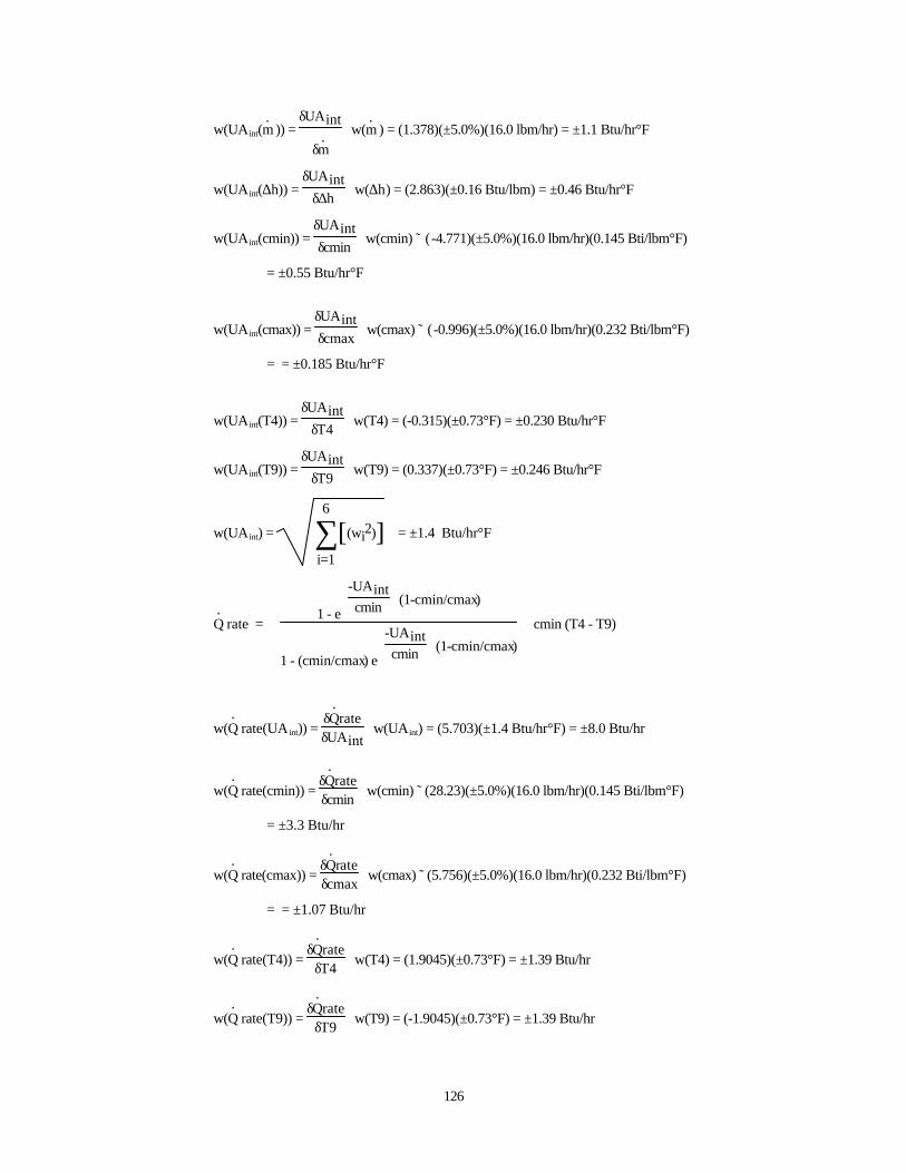
126

w(UAint(m. )) =

δUAint

δm. w(m

. ) = (1.378)(±5.0%)(16.0 lbm/hr) = ±1.1 Btu/hr°F

w(UAint(∆h)) = δUAint

δ∆h w(∆h) = (2.863)(±0.16 Btu/lbm) = ±0.46 Btu/hr°F

w(UAint(cmin)) = δUAintδcmin

w(cmin) ˜ (-4.771)(±5.0%)(16.0 lbm/hr)(0.145 Bti/lbm°F)

= ±0.55 Btu/hr°F

w(UAint(cmax)) = δUAintδcmax

w(cmax) ˜ (-0.996)(±5.0%)(16.0 lbm/hr)(0.232 Bti/lbm°F)

= = ±0.185 Btu/hr°F

w(UAint(T4)) = δUAint

δT4 w(T4) = (-0.315)(±0.73°F) = ±0.230 Btu/hr°F

w(UAint(T9)) = δUAint

δT9 w(T9) = (0.337)(±0.73°F) = ±0.246 Btu/hr°F

w(UAint) = ∑i=1

6

[ ](wi2) = ±1.4 Btu/hr°F

Q. rate =

1 - e

-UAint

cmin (1-cmin/cmax)

1 - (cmin/cmax) e

-UAint

cmin (1-cmin/cmax)

cmin (T4 - T9)

w(Q. rate(UA int)) =

δQ.rate

δUAint w(UAint) = (5.703)(±1.4 Btu/hr°F) = ±8.0 Btu/hr

w(Q. rate(cmin)) =

δQ.rate

δcmin w(cmin) ˜ (28.23)(±5.0%)(16.0 lbm/hr)(0.145 Bti/lbm°F)

= ±3.3 Btu/hr

w(Q. rate(cmax)) =

δQ.rate

δcmax w(cmax) ˜ (5.756)(±5.0%)(16.0 lbm/hr)(0.232 Bti/lbm°F)

= = ±1.07 Btu/hr

w(Q. rate(T4)) =

δQ.rate

δT4 w(T4) = (1.9045)(±0.73°F) = ±1.39 Btu/hr

w(Q. rate(T9)) =

δQ.rate

δT9 w(T9) = (-1.9045)(±0.73°F) = ±1.39 Btu/hr

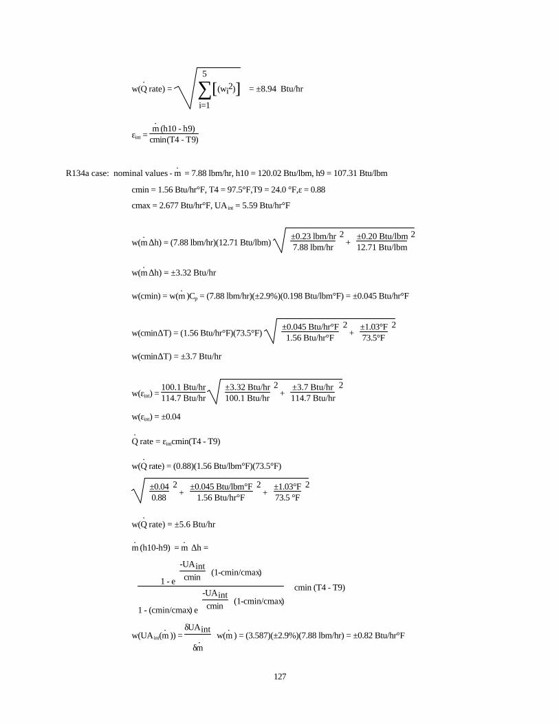
127

w(Q. rate) = ∑

i=1

5

[ ](wi2) = ±8.94 Btu/hr

εint = m. (h10 - h9)

cmin(T4 - T9)

R134a case: nominal values - m. = 7.88 lbm/hr, h10 = 120.02 Btu/lbm, h9 = 107.31 Btu/lbm

cmin = 1.56 Btu/hr°F, T4 = 97.5°F,T9 = 24.0 °F,ε = 0.88

cmax = 2.677 Btu/hr°F, UA int = 5.59 Btu/hr°F

w(m. ∆h) = (7.88 lbm/hr)(12.71 Btu/lbm)

±0.23 lbm/hr

7.88 lbm/hr2 +

±0.20 Btu/lbm

12.71 Btu/lbm2

w(m. ∆h) = ±3.32 Btu/hr

w(cmin) = w(m. )Cp = (7.88 lbm/hr)(±2.9%)(0.198 Btu/lbm°F) = ±0.045 Btu/hr°F

w(cmin∆T) = (1.56 Btu/hr°F)(73.5°F)

±0.045 Btu/hr°F

1.56 Btu/hr°F2 +

±1.03°F

73.5°F2

w(cmin∆T) = ±3.7 Btu/hr

w(εint) = 100.1 Btu/hr114.7 Btu/hr

±3.32 Btu/hr

100.1 Btu/hr2 +

±3.7 Btu/hr

114.7 Btu/hr2

w(εint) = ±0.04

Q. rate = εintcmin(T4 - T9)

w(Q. rate) = (0.88)(1.56 Btu/lbm°F)(73.5°F)

±0.04

0.882 +

±0.045 Btu/lbm°F

1.56 Btu/hr°F2 +

±1.03°F

73.5 °F2

w(Q. rate) = ±5.6 Btu/hr

m. (h10-h9) = m

. ∆h =

1 - e

-UAint

cmin (1-cmin/cmax)

1 - (cmin/cmax) e

-UAint

cmin (1-cmin/cmax)

cmin (T4 - T9)

w(UAint(m. )) =

δUAint

δm. w(m

. ) = (3.587)(±2.9%)(7.88 lbm/hr) = ±0.82 Btu/hr°F

128

w(UAint(∆h)) = δUAint

δ∆h w(∆h) = (2.224)(±0.20 Btu/lbm) = ±0.44 Btu/hr°F

w(UAint(cmin)) = δUAintδcmin

w(cmin) ˜ (-10.638)(±2.9%)(7.88 lbm/hr)(0.198 Bti/lbm°F)

= ±0.48 Btu/hr°F

w(UAint(cmax)) = δUAintδcmax

w(cmax) ˜ (-1.392)(±2.9%)(7.88 lbm/hr)(0.34 Bti/lbm°F)

= = ±0.11 Btu/hr°F

w(UAint(T4)) = δUAint

δT4 w(T4) = (-0.348)(±0.73°F) = ±0.25 Btu/hr°F

w(UAint(T9)) = δUAint

δT9 w(T9) = (0.382)(±0.73°F) = ±0.28 Btu/hr°F

w(UAint) = ∑i=1

6

[ ](wi2) = ±1.1 Btu/hr°F

Q. rate =

1 - e

-UAint

cmin (1-cmin/cmax)

1 - (cmin/cmax) e

-UAint

cmin (1-cmin/cmax)

cmin (T4 - T9)

w(Q. rate(UA int)) =

δQ.rate

δUAint w(UAint) = (3.68)(±1.1 Btu/hr°F) = ±4.05 Btu/hr

w(Q. rate(cmin)) =

δQ.rate

δcmin w(cmin) ˜ (41.657)(±2.9%)(7.88 lbm/hr)(0.198 Bti/lbm°F)

= ±1.88 Btu/hr

w(Q. rate(cmax)) =

δQ.rate

δcmax w(cmax) ˜ (5.1429)(±2.9%)(7.88 lbm/hr)(0.34 Bti/lbm°F)

= = ±0.40 Btu/hr

w(Q. rate(T4)) =

δQ.rate

δT4 w(T4) = (1.392)(±0.73°F) = ±1.02 Btu/hr

w(Q. rate(T9)) =

δQ.rate

δT9 w(T9) = (-1.392)(±0.73°F) = ±1.02 Btu/hr

w(Q. rate) = ∑

i=1

5

[ ](wi2) = ±4.71 Btu/hr

129

Evaporator Volumetric Air Flow Rate Uncertainty

ρCp60V. e∆T = m

. (h10 - h4) = Q

. e

m. fz h(Tfz) + m

. ff h(Tff) = m

. a h(Tma)

3.413P. fan = m

. a Cp (Tfanout - Taevapout)

m. a = m

. fz + m

. ff

m. a = ρ60V

. e

a = m.fz

m.a

R12 nominal values: m. = 18.12 lbm/hr, h10 = 88.95 Btu/lbm, h4 = 28.83 Btu/lbm

Tfz = 42.3°F, Tff = 59.4°F, P. fan = 12.0 W, a = 0.871

Tfanout = 29.8°F, Tma = 44.41°F, Taevapout = 29.23°F

V. e = 62.6 ft3/min, ρ = 0.079 lbm/ft3, Cp = 0.24 Btu/lbm°F

w(V. e(m

. )) =

δV.e

δm. w(m

. ) = (3.59)(±5.0%)(18.12 lbm/hr) = ±3.25 ft3/min

w(V. e(∆h)) =

δV.e

δ∆h w(∆h) = (1.07)(±0.16 Btu/lbm) = ±0.17 ft3/min

w(V. e(Tfz)) =

δV.e

δTfz w(Tfz) = (-3.62)(±0.73°F) = ±2.64 ft3/min

w(V. e(Tff)) =

δV.e

δTff w(Tff) = (-5.48e-1)(±0.73°F) = ±0.40 ft3/min

w(V. e(P

. fan)) =

δV.e

δP.fan

w(P. fan) = (-2.04e-1)(±0.5W) = ±0.10 ft3/min

w(V. e(Tfanout)) =

δV.e

δTfanout w(Tfanout) = (4.35)(±0.73°F) = ±3.18 ft3/min

w(V. e) = ∑

i=1

6

[ ](wi2) = ±5.3 ft3/min

130

w(a(m. )) =

δa

δm. w(m

. ) = (-4.93e-2)(±5.0%)(18.12 lbm/hr) = ±0.045

w(a(∆h)) = δa

δ∆h w(∆h) = (-1.47e-2)(±0.16 Btu/lbm) = ±0.0024

w(a(Tfz)) = δa

δTfz w(Tfz) = (5.22e-2)(±0.73°F) = ±0.0038

w(a(Tff)) = δa

δTff w(Tff) = (7.3e-3)(±0.73°F) = ±0.0053

w(a(P. fan)) =

δa

δP.fan

w(P. fan) = (2.8e-3)(±0.5W) = ±0.0014

w(a(Tfanout)) = δa

δTfanout w(Tfanout) = (-5.84e-2)(±0.73°F) = ±0.0426

w(a) = ∑i=1

6

[ ](wi2) = ±0.062

w(Tma(m. )) =

δTma

δm. w(m

. ) = (8.61e-11)(±5.0%)(18.12 lbm/hr) ˜ 0.0°F

w(Tma(∆h)) = δTmaδ∆h

w(∆h) = (2.57e-11)(±0.16 Btu/lbm) ˜ 0.0°F

w(Tma(Tfz)) = δTmaδTfz

w(Tfz) = (8.71e-1)(±0.73°F) = ±0.636°F

w(Tma(Tff)) = δTmaδTff

w(Tff) = (1.29e-1)(±0.73°F) = ±0.0942°F

w(Tma(P. fan)) =

δTma

δP.fan

w(P. fan) = (-4.95e-12)(±0.5W) ˜ 0.0°F

w(Tma(Tfanout)) = δTma

δTfanout w(Tfanout) = (1.05e-10)(±0.73°F) ˜ 0.0°F

w(Tma) = ∑i=1

6

[ ](wi2) = ±0.64°F

w(Q. e) = (18.12 lbm/hr)(60.12 Btu/lbm)

±0.91 lbm/hr

18.12 lbm/hr2 +

±0.24 Btu.lbm

60.12 Btu/lbm2

w(Q. e) = ±54.9 Btu/hr

131

R134a nominal values: m. = 7.69 lbm/hr, h10 = 115.59 Btu/lbm, h4 = 33.55 Btu/lbm

Tfz = 32.3°F, Tff = 55.0°F, P. fan = 12.5 W, Cp = 0.24 Btu/lbm°F

ρ = 0.078 lbm/ft3, Tfanout = 25.9°F, Tma = 34.6°F

Taevapout = 25.28°F, V. e = 60.2 ft3/min, a = 0.899

w(V. e(m

. )) =

δV.e

δm. w(m

. ) = (8.40)(±2.9%)(7.69 lbm/hr) = ±1.87 ft3/min

w(V. e(∆h)) =

δV.e

δ∆h w(∆h) = (7.79e-1)(±0.20 Btu/lbm) = ±0.16 ft3/min

w(V. e(Tfz)) =

δV.e

δTfz w(Tfz) = (-6.02)(±0.73°F) = ±4.39 ft3/min

w(V. e(Tff)) =

δV.e

δTff w(Tff) = (-6.97e-1)(±0.73°F) = ±0.51 ft3/min

w(V. e(P

. fan)) =

δV.e

δP.fan

w(P. fan) = (-3.49e-1)(±0.5W) = ±0.175 ft3/min

w(V. e(Tfanout)) =

δV.e

δTfanout w(Tfanout) = (7.14)(±0.73°F) = ±5.2 ft3/min

w(V. e) = ∑

i=1

6

[ ](wi2) = ±7.1 ft3/min

w(a(m. )) =

δa

δm. w(m

. ) = (-5.34e-2)(±2.9%)(7.69 lbm/hr) = ±0.012

w(a(∆h)) = δa

δ∆h w(∆h) = (-4.95e-3)(±0.20 Btu/lbm) = ±0.001

w(a(Tfz)) = δa

δTfz w(Tfz) = (4.01e-2)(±0.73°F) = ±0.029

w(a(Tff)) = δa

δTff w(Tff) = (4.35e-3)(±0.73°F) = ±0.0032

w(a(P. fan)) =

δa

δP.fan

w(P. fan) = (2.22e-3)(±0.5W) = ±0.0011

w(a(Tfanout)) = δa

δTfanout w(Tfanout) = (-4.40e-2)(±0.73°F) = ±0.032

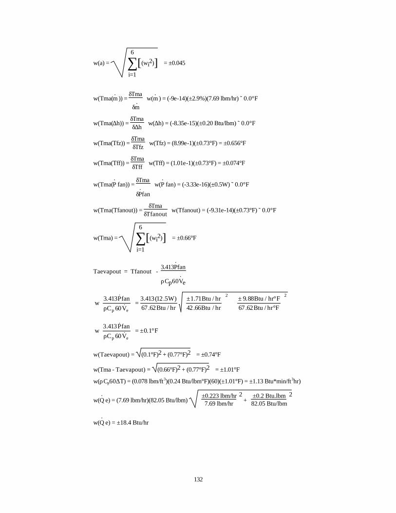
132

w(a) = ∑i=1

6

[ ](wi2) = ±0.045

w(Tma(m. )) =

δTma

δm. w(m

. ) = (-9e-14)(±2.9%)(7.69 lbm/hr) ˜ 0.0°F

w(Tma(∆h)) = δTmaδ∆h

w(∆h) = (-8.35e-15)(±0.20 Btu/lbm) ˜ 0.0°F

w(Tma(Tfz)) = δTmaδTfz

w(Tfz) = (8.99e-1)(±0.73°F) = ±0.656°F

w(Tma(Tff)) = δTmaδTff

w(Tff) = (1.01e-1)(±0.73°F) = ±0.074°F

w(Tma(P. fan)) =

δTma

δP.fan

w(P. fan) = (-3.33e-16)(±0.5W) ˜ 0.0°F

w(Tma(Tfanout)) = δTma

δTfanout w(Tfanout) = (-9.31e-14)(±0.73°F) ˜ 0.0°F

w(Tma) = ∑i=1

6

[ ](wi2) = ±0.66°F

Taevapout = Tfanout - 3.413P

.fan

ρCp60V.e

22

ep Fhr/Btu62.67Fhr/Btu88.9

hr/Btu66.42hr/Btu71.1

hr/Btu62.67)W5.12(413.3

V60CfanP413.3

w

°°±

+

±

=

ρ &&

F1.0V60CfanP413.3

wep

°±=

ρ &&

w(Taevapout) = (0.1°F)2 + (0.77°F)2 = ±0.74°F

w(Tma - Taevapout) = (0.66°F)2 + (0.77°F)2 = ±1.01°F

w(ρCp60∆T) = (0.078 lbm/ft3)(0.24 Btu/lbm°F)(60)(±1.01°F) = ±1.13 Btu*min/ft3hr)

w(Q. e) = (7.69 lbm/hr)(82.05 Btu/lbm)

±0.223 lbm/hr

7.69 lbm/hr2 +

±0.2 Btu.lbm

82.05 Btu/lbm2

w(Q. e) = ±18.4 Btu/hr

133

Evaporator Conductances and Heat Transfer Uncertainties

R12: nominal values : Q. e = 1089 Btu/hr, Q

. sup = 85.0 Btu/hr, Q

. 2ph = 1004 Btu/hr

m. = 18.12 lbm/hr, cmin = 2.62 Btu/hr°F, casup = 68.7 Btu/hr°F

Tma = 44.0 °F, T7 = -0.2°F, a2ph = 1.46 ft2, asup = 2.34 ft2

ca2ph = 52.7 Btu/hr°F,h4 = 28.8 Btu/lbm, h8 = 77.25 Btu/lbm

h9 = 81.96 Btu/lbm, h10 = 88.95 Btu/lbm, Usup = 1.579 Btu/hr-ft2°F

U2ph = 20.51 Btu/hr-ft2°F

Superheated section

m. (h9-h8) = m

. ∆h =

1 - e

-Usup asup

cmin (1+cmin/casup)

1 + (cmin/casup) cmin (Tma - T7)

w(Usup(m. )) =

δUsup

δm. w(m

. ) = (1.97e-1)(±5.0%)(18.12 lbm/hr) = ±0.18 Btu/hr°F*ft2

w(Usup(∆h)) = δUsup

δ∆h w(∆h) = (7.51e-1)(±0.16 Btu/lbm) = ±0.12 Btu/hr°F*ft2

w(Usup(cmin)) = δUsupδcmin

w(cmin) ˜ (-6.98e-1)(±5.0%)(18.12 lbm/hr)(0.14 Bti/lbm°F)

= ±0.088 Btu/hr°F*ft2

w(Usup(casup)) = δUsupδcasup

w(casup)

˜ (-1.03e-3)(0.079 lbm/ft3)(0.24 Btu/lbm°F)(60)(±7.1 ft3min) = ±0.008 Btu/hr°F*ft2

w(Usup(Tma)) = δUsupδTma

w(Tma) = (-7.75e-2)(±0.64°F) = ±0.05 Btu/hr°F*ft2

w(Usup(T7)) = δUsup

δT7 w(T7) = (7.95e-2)(±0.73°F) = ±0.058 Btu/hr°F*ft2

w(Usup) = ∑i=1

6

[ ](wi2) = ±0.25 Btu/hr°F*ft2

Two-phase section

m. (h8-h7) = 1 - e

(-U2ph a2ph/ca2ph) ca2ph (Tma - T7)

w(U2ph(m. )) =

δU2ph

δm. w(m

. ) = (1.53)(±5.0%)(18.12 lbm/hr) = ±1.39 Btu/hr°F*ft2

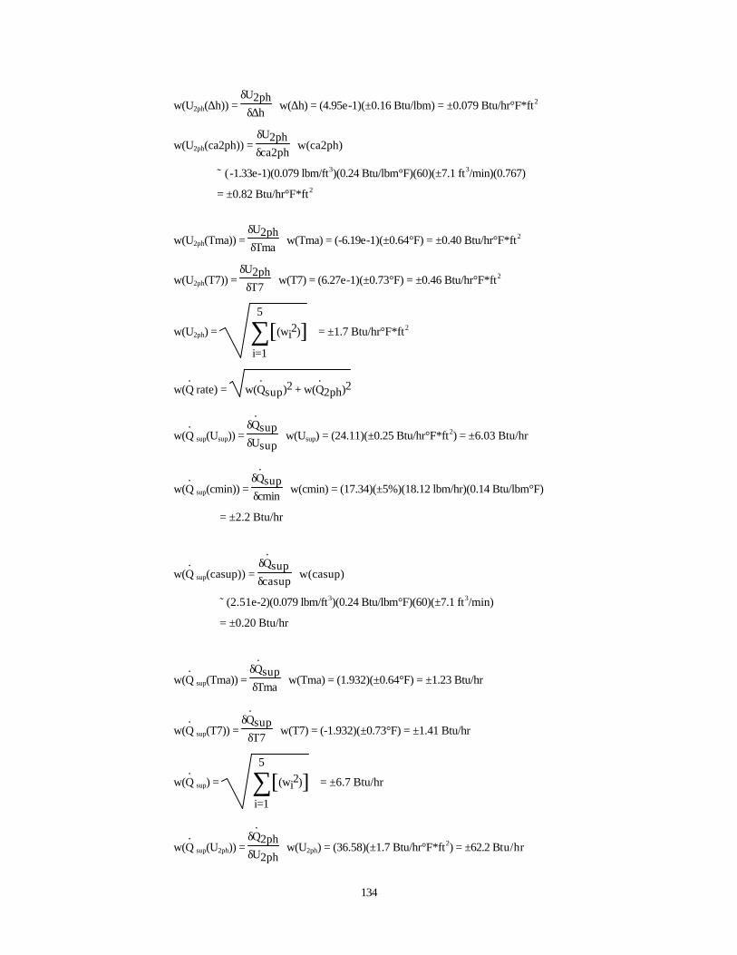
134

w(U2ph(∆h)) = δU2ph

δ∆h w(∆h) = (4.95e-1)(±0.16 Btu/lbm) = ±0.079 Btu/hr°F*ft2

w(U2ph(ca2ph)) = δU2phδca2ph

w(ca2ph)

˜ (-1.33e-1)(0.079 lbm/ft3)(0.24 Btu/lbm°F)(60)(±7.1 ft3/min)(0.767)

= ±0.82 Btu/hr°F*ft2

w(U2ph(Tma)) = δU2phδTma

w(Tma) = (-6.19e-1)(±0.64°F) = ±0.40 Btu/hr°F*ft2

w(U2ph(T7)) = δU2ph

δT7 w(T7) = (6.27e-1)(±0.73°F) = ±0.46 Btu/hr°F*ft2

w(U2ph) = ∑i=1

5

[ ](wi2) = ±1.7 Btu/hr°F*ft2

w(Q. rate) = w(Q

.sup)2 + w(Q

.2ph)2

w(Q. sup(Usup)) =

δQ.sup

δUsup w(Usup) = (24.11)(±0.25 Btu/hr°F*ft2) = ±6.03 Btu/hr

w(Q. sup(cmin)) =

δQ.sup

δcmin w(cmin) = (17.34)(±5%)(18.12 lbm/hr)(0.14 Btu/lbm°F)

= ±2.2 Btu/hr

w(Q. sup(casup)) =

δQ.sup

δcasup w(casup)

˜ (2.51e-2)(0.079 lbm/ft3)(0.24 Btu/lbm°F)(60)(±7.1 ft3/min)

= ±0.20 Btu/hr

w(Q. sup(Tma)) =

δQ.sup

δTma w(Tma) = (1.932)(±0.64°F) = ±1.23 Btu/hr

w(Q. sup(T7)) =

δQ.sup

δT7 w(T7) = (-1.932)(±0.73°F) = ±1.41 Btu/hr

w(Q. sup) = ∑

i=1

5

[ ](wi2) = ±6.7 Btu/hr

w(Q. sup(U2ph)) =

δQ.2ph

δU2ph w(U2ph) = (36.58)(±1.7 Btu/hr°F*ft2) = ±62.2 Btu/hr

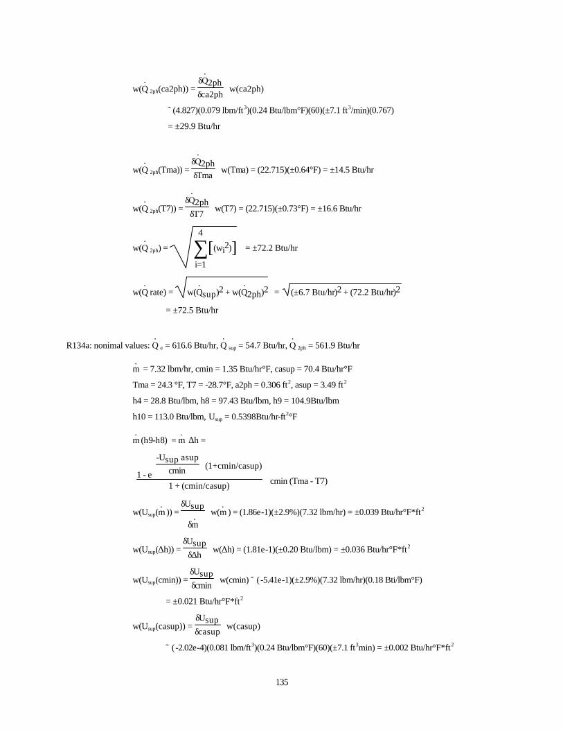
135

w(Q. 2ph(ca2ph)) =

δQ.2ph

δca2ph w(ca2ph)

˜ (4.827)(0.079 lbm/ft3)(0.24 Btu/lbm°F)(60)(±7.1 ft3/min)(0.767)

= ±29.9 Btu/hr

w(Q. 2ph(Tma)) =

δQ.2ph

δTma w(Tma) = (22.715)(±0.64°F) = ±14.5 Btu/hr

w(Q. 2ph(T7)) =

δQ.2ph

δT7 w(T7) = (22.715)(±0.73°F) = ±16.6 Btu/hr

w(Q. 2ph) = ∑

i=1

4

[ ](wi2) = ±72.2 Btu/hr

w(Q. rate) = w(Q

.sup)2 + w(Q

.2ph)2 = (±6.7 Btu/hr)2 + (72.2 Btu/hr)2

= ±72.5 Btu/hr

R134a: nonimal values: Q. e = 616.6 Btu/hr, Q

. sup = 54.7 Btu/hr, Q

. 2ph = 561.9 Btu/hr

m. = 7.32 lbm/hr, cmin = 1.35 Btu/hr°F, casup = 70.4 Btu/hr°F

Tma = 24.3 °F, T7 = -28.7°F, a2ph = 0.306 ft2, asup = 3.49 ft2

h4 = 28.8 Btu/lbm, h8 = 97.43 Btu/lbm, h9 = 104.9Btu/lbm

h10 = 113.0 Btu/lbm, Usup = 0.5398Btu/hr-ft2°F

m. (h9-h8) = m

. ∆h =

1 - e

-Usup asup

cmin (1+cmin/casup)

1 + (cmin/casup) cmin (Tma - T7)

w(Usup(m. )) =

δUsup

δm. w(m

. ) = (1.86e-1)(±2.9%)(7.32 lbm/hr) = ±0.039 Btu/hr°F*ft2

w(Usup(∆h)) = δUsup

δ∆h w(∆h) = (1.81e-1)(±0.20 Btu/lbm) = ±0.036 Btu/hr°F*ft2

w(Usup(cmin)) = δUsupδcmin

w(cmin) ˜ (-5.41e-1)(±2.9%)(7.32 lbm/hr)(0.18 Bti/lbm°F)

= ±0.021 Btu/hr°F*ft2

w(Usup(casup)) = δUsupδcasup

w(casup)

˜ (-2.02e-4)(0.081 lbm/ft3)(0.24 Btu/lbm°F)(60)(±7.1 ft3min) = ±0.002 Btu/hr°F*ft2

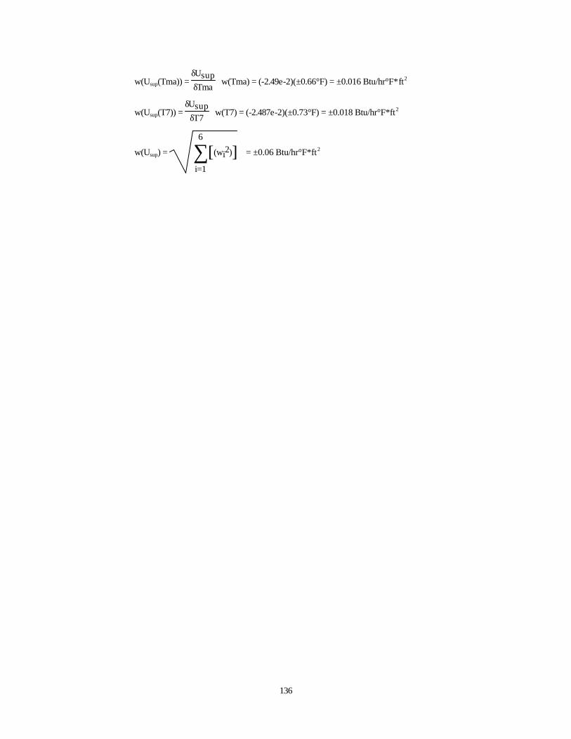
136

w(Usup(Tma)) = δUsupδTma

w(Tma) = (-2.49e-2)(±0.66°F) = ±0.016 Btu/hr°F*ft2

w(Usup(T7)) = δUsup

δT7 w(T7) = (-2.487e-2)(±0.73°F) = ±0.018 Btu/hr°F*ft2

w(Usup) = ∑i=1

6

[ ](wi2) = ±0.06 Btu/hr°F*ft2

137

Appendix E: Program Listings

E.E.S. Worksheet - Model determines the convective heat transfer coefficient for the compressor by comparing the

refrigerant side energy balance with the air side temperature difference. A non-linear least squares method is used to

find the optimum. Dean M. Staley

Vdotcond = 115.8 DUPLICATE i=1,33 Pfan[i] = lookup(i,13) Pcomp[i] = lookup(i,12) Psystem[i] = lookup(i,11) Tconfanout[i] = lookup(i,8) P1[i] = lookup(i,14) T1[i] = lookup(i,15) P10[i] = lookup(i,22) T10[i] = lookup(i,23) w[i] = lookup(i,27) h1[i] = Enthalpy(R12,T=T1[i],P=P1[i]+14.4) h10[i] = Enthalpy(R12,T=T10[i],P=P10[i]+14.4) rho[i] = 1/Volume(Air,T=Tconfanout[i],P=14.4) Cpair[i] = SpecHeat(Air,T=Tconfanout[i]) Pconfan[i] = Psystem[i]-Pcomp[i]-Pfan[i] (Pconfan[i]*3.413) = rho[i]*Cpair[i]*Vdotcond*60*(Tconfanout[i]-Taircomp[i]) Qcomp[i] = (Pcomp[i]*3.413)-w[i]*(h1[i]-h10[i]) dPhbar[i] = (Qcomp[i]-hbar*(T1[i]-Taircomp[i]))*(-(T1[i]-Taircomp[i])) error[i] = (Qcomp[i]-hbar*(T1[i]-Taircomp[i]))^2 percenterr[i] = sqrt(error[i])/Qcomp[i] END sum(dPhbar[i],i=1,33) = 0.0 totalerr = sum(error[i],i=1,33)

******************************************************************

E.E.S. Worksheet - Model determines the best UA or effectiveness for the interchanger by the comparing refrigerant energy side balance with the rate equation for the interchanger. Data for cases with subcooling at the cap-tube inlet and superheat at the evaporator outlet are used. A nonlinear least squares approach is used.Dean M. Staley DUPLICATE i=1,10 P9[i] = lookup(i,20) T9[i] = lookup(i,21) P10[i] = lookup(i,22) T10[i] = lookup(i,23) T4[i] = lookup(i,25) w[i] = lookup(i,27) h4[i] = Enthalpy(R12,T=T4[i],X=0.0) h9[i] = Enthalpy(R12,T=T9[i],P=P9[i]+14.4) h6[i] = h4 [i] - (h10[i]-h9[i])

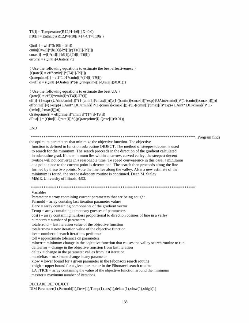
138

T6[i] = Temperature(R12,H=h6[i],X=0.0) h10[i] = Enthalpy(R12,P=P10[i]+14.4,T=T10[i]) Qint[i] = w[i]*(h10[i]-h9[i]) cmin[i]=w[i]*(h10[i]-h9[i])/(T10[i]-T9[i]) cmax[i]=w[i]*(h4[i]-h6[i])/(T4[i]-T6[i]) error[i] = (Qint[i]-Qrate[i])^2 Use the following equations to estimate the best effectiveness Qrate[i] = eff*cmin[i]*(T4[i]-T9[i]) Qrateprime[i] = eff*1.01*cmin[i]*(T4[i]-T9[i]) dPeff[i] = (Qint[i]-Qrate[i])*(-((Qrateprime[i]-Qrate[i])/0.01)) Use the following equations to estimate the best UA Qrate[i] = eff[i]*cmin[i]*(T4[i]-T9[i]) eff[i]=(1-exp(-(UAint/cmin[i])*(1-(cmin[i]/cmax[i]))))/(1-((cmin[i]/cmax[i])*exp(-(UAint/cmin[i])*(1-(cmin[i]/cmax[i]))))) effprime[i]=(1-exp(-(UAint*1.01/cmin[i])*(1-(cmin[i]/cmax[i]))))/(1-((cmin[i]/cmax[i])*exp(-(UAint*1.01/cmin[i])*(1-(cmin[i]/cmax[i]))))) Qrateprime[i] = effprime[i]*cmin[i]*(T4[i]-T9[i]) dPua[i] = (Qint[i]-Qrate[i])*(-((Qrateprime[i]-Qrate[i])/0.01)) END !*****************************************************************************! Program finds the optimum parameters that minimize the objective function. The objective ! function is defined in function subroutine OBJECT. The method of steepest-decent is used ! to search for the minimum. The search proceeds in the direction of the gradient calculated ! in subroutine grad. If the minimum lies within a narrow, curved valley, the steepest-decent ! routine will not converge in a reasonable time. To speed convergence in this case, a minimum ! at a point close to the current point is determined. The search then proceeds along the line ! formed by these two points. Note the line lies along the valley. After a new estimate of the ! minimum is found, the steepest-descent routine is continued. Dean M. Staley ! M&IE, University of Illinois, 4/92. ! !*****************************************************************************! ! Variables ! Parameter = array containing current parameters that are being sought ! Parmold = array containg last iteration parameter values ! Derv = array containing components of the gradient vector ! Temp = array containing temporary guesses of parameters ! cos() = array containing numbers proportional to direction cosines of line in a valley ! numparm = number of parameters ! totalerrold = last iteration value of the objective function ! totalerrnew = new iteration value of the objective function ! iter = number of search iterations performed ! toll = approximate tolerance on parameters ! minerr = minimum change in the objective function that causes the valley search routine to run ! deltaerror = change in the objective function from last iteration ! deltax = change in the parameter values from last iteration ! maxdeltax = maximum change in any parameter ! xlow = lower bound for a given parameter in the Fibonacci search routine ! xhigh = upper bound for a given parameter in the Fibonacci search routine ! LATTICE = array containing the value of the objective function around the minimum ! maxiter = maximum number of iterations ! DECLARE DEF OBJECT DIM Parameter(1),Parmold(1),Derv(1),Temp(1),cos(1),deltax(1),xlow(1),xhigh(1)

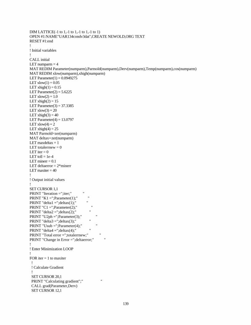
139

DIM LATTICE(-1 to 1,-1 to 1,-1 to 1,-1 to 1) OPEN #1:NAME"UAR134condv3dat",CREATE NEWOLD,ORG TEXT RESET #1:end ! ! Initial variables ! CALL initial LET numparm = 4 MAT REDIM Parameter(numparm),Parmold(numparm),Derv(numparm),Temp(numparm),cos(numparm) MAT REDIM xlow(numparm),xhigh(numparm) LET Parameter(1) = 0.0949275 LET xlow(1) = 0.05 LET xhigh(1) = 0.15 LET Parameter(2) = 5.6225 LET xlow(2) = 1.0 LET xhigh(2) = 15 LET Parameter(3) = 37.3385 LET xlow(3) = 20 LET xhigh(3) = 40 LET Parameter(4) = 13.0797 LET xlow(4) = 2 LET xhigh(4) = 25 MAT Parmold=zer(numparm) MAT deltax=zer(numparm) LET maxdeltax = 1 LET totalerrnew = 0 LET iter = 0 LET toll = 1e-4 LET minerr = 0.1 LET deltaerror = 2*minerr LET maxiter = 40 ! ! Output initial values ! SET CURSOR 1,1 PRINT "Iteration =";iter;" " PRINT "K1 =";Parameter(1);" " PRINT "delta1 =";deltax(1);" " PRINT "C1 =";Parameter(2);" " PRINT "delta2 =";deltax(2);" " PRINT "U2ph =";Parameter(3);" " PRINT "delta3 =";deltax(3);" " PRINT "Usub =";Parameter(4);" " PRINT "delta4 =";deltax(4);" " PRINT "Total error =";totalerrnew;" " PRINT "Change in Error =";deltaerror;" " ! ! Enter Minimization LOOP ! FOR iter = 1 to maxiter ! ! Calculate Gradient ! SET CURSOR 20,1 PRINT "Calculating gradient";" " CALL grad(Parameter,Derv) SET CURSOR 12,1

140

PRINT "Derivative 1 =";Derv(1);" " PRINT "Derivative 2 =";Derv(2);" " PRINT "Derivative 3 =";Derv(3);" " PRINT "Derivative 4 =";Derv(4);" " ! ! Output data to a file ! PRINT #1:iter;",";Parameter(1);",";Parameter(2);",";Parameter(3);",";Parameter(4);",";totalerrnew;",";deltaerror PRINT #1:" ";Derv(1);",";Derv(2);",";Derv(3);",";Derv(4) ! ! Start search ! IF ABS(deltaerror) < minerr AND maxdeltax < toll THEN ! In possible valley - Find another minimum point and search ! in direction of line formed by last minimum and new minimum SET CURSOR 20,1 ! Find new minimum close to old point PRINT "Running valley search";" " PRINT #1:"Running valley search" LET Temp(1) = Parameter(1) IF Derv(2) > 0.0 THEN LET Temp(2) = 0.99*Parameter(2) ELSE LET Temp(2) = 1.01*Parameter(2) END IF LET Temp(3) = Parameter(3) LET Temp(4) = Parameter(4) CALL fibonacci(Temp,xlow,xhigh,Derv,1,toll) CALL fibonacci(Temp,xlow,xhigh,Derv,3,toll) CALL fibonacci(Temp,xlow,xhigh,Derv,4,toll) ! ! Calculate numbers proportional to the direction cosines of line ! LET cos(1) = (Temp(1)-Parameter(1))/toll LET cos(2) = (Temp(2)-Parameter(2))/toll LET cos(3) = (Temp(3)-Parameter(3))/toll LET cos(4) = (Temp(4)-Parameter(4))/toll ! ! Search in this direction ! CALL fibonacci(Parameter,xlow,xhigh,cos,999,toll) SET CURSOR 20,1 PRINT " " ELSE !do steepest-decent ! ! Calculate new parameters in direction of gradient ! SET CURSOR 20,1 PRINT "Running Parameter Search";" " CALL fibonacci(Parameter,xlow,xhigh,Derv,999,toll) SET CURSOR 20,1 PRINT " " END IF ! ! Update Variables and Output New Results ! LET totalerrold = totalerrnew

141

LET totalerrnew = OBJECT(Parameter) LET deltaerror = totalerrnew-totalerrold FOR i = 1 to numparm LET deltax(i) = Parameter(i) - Parmold(i) LET Parmold(i) = Parameter(i) NEXT i LET maxdeltax = 0.0 FOR i = 1 to numparm IF ABS(deltax(i)) > maxdeltax THEN LET maxdeltax = ABS(deltax(i)) NEXT i SET CURSOR 1,1 PRINT "Iteration =";iter;" " PRINT "K1 =";Parameter(1);" " PRINT "delta1 =";deltax(1);" " PRINT "C1 =";Parameter(2);" " PRINT "delta2 =";deltax(2);" " PRINT "U2ph =";Parameter(3);" " PRINT "delta3 =";deltax(3);" " PRINT "Usub =";Parameter(4);" " PRINT "delta4 =";deltax(4);" " PRINT "Total error =";totalerrnew;" " PRINT "Change in Error =";deltaerror;" " NEXT iter ! ! Output last iteration to file ! PRINT #1:iter;",";Parameter(1);",";Parameter(2);",";Parameter(3);",";Parameter(4);",";totalerrnew;",";deltaerror PRINT #1:Derv(1);",";Derv(2);",";Derv(3);",";Derv(4) ! ! Run short exhaustive search around minimum ! FOR i = -1 to 1 FOR j = -1 to 1 FOR k = -1 to 1 FOR l = -1 to 1 LET Temp(1) = Parameter(1) + Parameter(1)*i*toll*100 LET Temp(2) = Parameter(2) + Parameter(2)*j*toll*100 LET Temp(3) = Parameter(3) + Parameter(3)*k*toll*100 LET Temp(4) = Parameter(4) + Parameter(4)*l*toll*100 LET LATTICE(i,j,k,l) = OBJECT(Temp) PRINT #1:LATTICE(i,j,k,l); NEXT l NEXT k NEXT j NEXT i ! CLOSE #1 ! END ! ! ! MODULE Fibonacci SUB fibonacci(Parameter(),lowbd(),highbd(),Derv(),optvar,toll) ! ! Subroutine performs a univariate Fibonacci search for the parameter eaual to optvar i.e. ! if optvar equals 2 then search for the second parameter. The subroutine was written to minimize

142

! the objective funtion defined by the function routine OBJECT. The routine could be easily extended ! to maximize a given objective function. If optvar equals 999 the routine performs a univariate ! search in the directions specified by the derivatives Derv(). In this way the search can proceed ! along directions that are not parallel to the parameter axes. Dean M. Staley 4/92 ! ! Variables ! ! Parameter = array containging the parameters in the objective function ! lowbd = array containing lower bounds on the parameters ! highbd = array containing upper bounds on the parameters ! xlow = lower bound of specified search parameter for given iteration ! xhigh = upper bound of specified search parameter for given iteration ! Derv = array containing derivatives proportional to direction cosines ! optvar = number specifying which optimum parameter is to be determined ! toll = approximate tolerance of the final value of the specified parameter ! numparm = number of total parameters ! F = array containing Fibonacci numbers ! Temp = array containing temporary estimates of parameters ! OBJECT = objective function routine - specified outside module ! xleft = point nearest to xlow ! xright = point nearest to xhigh ! yleft = value of objective function at xleft ! yright = value of objective funtion at xright ! Int = interval within which to search for minimum ! DIM Temp(1),F(0 to 99) DECLARE DEF OBJECT LET numparm = SIZE(Parameter) MAT REDIM Temp(numparm) ! IF optvar = 999 THEN LET pivot = 1 LET xlow = lowbd(pivot) LET xhigh = highbd(pivot) ELSE LET xlow = lowbd(optvar) LET xhigh = highbd(optvar) END IF ! ! Calculate approximate Fibonacci number ! LET Fib = (xhigh-xlow)/toll ! ! Search for actual Fibonacci number ! LET F(0) = 1 LET F(1) = 1 LET n = 1 DO WHILE Fib > F(n) LET F(n+1) = F(n-1) + F(n) LET n = n+1 LOOP ! ! Start minimization routine ! LET Int = xhigh - xlow LET iter = 0.0

143

! FOR i = 2 to n IF i = 2 THEN LET xright = xlow + Int*(F(n-1)/F(n)) LET x = xright CALL reassign(x,Temp,Parameter,Derv,optvar,lowbd,highbd,pivot) LET yright = OBJECT(Temp) LET xleft = xlow + Int*(1-(F(n-1)/F(n))) LET x = xleft CALL reassign(x,Temp,Parameter,Derv,optvar,lowbd,highbd,pivot) LET yleft = OBJECT(Temp) ELSE IF i > 2 AND i < n THEN IF xhigh = xright THEN LET x = xlow + Int*(1-((xleft-xlow)/Int)) CALL reassign(x,Temp,Parameter,Derv,optvar,lowbd,highbd,pivot) LET y = OBJECT(Temp) IF x < xleft THEN LET xright = xleft LET yright = yleft LET xleft = x LET yleft = y ELSE LET xleft = x LET yleft = y END IF ELSE LET x = xlow + Int*(1-((xright-xlow)/Int)) CALL reassign(x,Temp,Parameter,Derv,optvar,lowbd,highbd,pivot) LET y = OBJECT(Temp) IF x > xright THEN LET xleft = xright LET yleft = yright LET xright = x LET yright = y ELSE LET xleft = x LET yleft = y END IF END IF ELSE IF xleft = xlow THEN LET xleft = xright - 0.01*toll LET x = xleft CALL reassign(x,Temp,Parameter,Derv,optvar,lowbd,highbd,pivot) LET yleft = OBJECT(Temp) ELSE LET xright = xleft + 0.01*toll LET x = xright CALL reassign(x,Temp,Parameter,Derv,optvar,lowbd,highbd,pivot) LET yright = OBJECT(Temp) END IF END IF IF yright > yleft THEN LET xhigh = xright ELSE LET xlow = xleft END IF

144

LET Int = xhigh - xlow LET iter = iter +1 SET CURSOR 21,1 PRINT "Iteration =";iter;" " NEXT i SET CURSOR 21,1 PRINT " " ! ! Update Parameters ! IF optvar = 999 THEN LET minx = (xhigh+xlow)/2 LET scale = (minx-Parameter(pivot))/Derv(pivot) FOR i = 1 to numparm IF i <> pivot THEN LET Parameter(i) = scale*Derv(i)+Parameter(i) NEXT i LET Parameter(pivot) = minx ELSE LET Parameter(optvar) = (xhigh+xlow)/2 END IF END SUB ! SUB reassign(x,Temp(),Parameter(),Derv(),optvar,lowbd(),highbd(),pivot) LET numparm = SIZE(Parameter) IF optvar = 999 THEN LET Temp(pivot) = x LET scale = (Temp(pivot)-Parameter(pivot))/Derv(pivot) FOR i = 1 to numparm IF i <> pivot THEN LET Temp(i) = scale*Derv(i)+Parameter(i) NEXT i ELSE LET Temp(optvar) = x FOR i = 1 to numparm IF i<> optvar THEN LET Temp(i) = Parameter(i) NEXT i END IF ! ! Check bounds ! FOR i = 1 to numparm IF Temp(i) < lowbd(i) OR Temp(i) > highbd(i) THEN PRINT "Parameters out of bounds in subroutine Fibonacci - adjust bounds" PRINT "Pivot variable =";pivot PRINT "Scale =";scale PRINT "Variable out of bounds = #";i FOR j = 1 to numparm PRINT "Variable #";j;" =";Temp(j) PRINT "Derivative #";j;" =";Derv(j) NEXT j STOP END IF NEXT i END SUB ! END MODULE ! !

145

SUB grad(Parameter(),Derv()) ! ! Subroutine calculates the gradient at the point specified by Parameter(). ! ! Variables ! Temp = array containing temporary values of parameters ! numparm = number of parameters ! deltak = increment in temporary parameters ! Parameter = array containg actual parameters ! Derv = array containg gradient components ! DECLARE DEF OBJECT DIM Temp(1) LET numparm = SIZE(Parameter) MAT REDIM Temp(numparm) LET deltak = 0.000001 LET F = OBJECT(Parameter) FOR i = 1 to numparm LET Temp(i) = Parameter(i) NEXT i ! FOR i = 1 to numparm LET Temp(i) = Parameter(i) + deltak LET Derv(i) = (OBJECT(Temp)-F)/deltak LET Temp(i) = Temp(i) - deltak NEXT i END SUB ! ! SUB initial ! ! Subroutine initializes variables for use in subroutine calcr - R134a condenser ! ! Variables ! w = refrigerant mass flow rate lbm/hr ! h1 = enthalpy of refrigerant at inlet of condenser Btu/lbm ! h1satvap = saturated vapor enthalpy at the condenser inlet pressure Btu/lbm ! h2 = saturated liquid enthalpy at the end of the two phase section Btu/lbm ! h3 = enthalpy of liquid refrigerant leaving condenser at the condenser outlet pressure Btu/lbm ! T1 = inlet tempeature to the condenser °F ! T2 = saturated condensing temperature °F ! cmin = mdot*Cp for desuperheating section Btu/hr°F ! cminsub = mdot Cp for subcooled section Btu/hr°F ! cacond = mdotair*Cpair for the condenser air flow rate Btu/hr°F ! Tconairin = condenser inlet air temperature °F ! numpt = number of data points ! hdesup = refrigerant side film coefficient for the despuerheating section Btu/ft^2-hr°R ! h2ph = refrigerant side film coefficient for the two-phase section Btu/ft^2-hr°R ! hsub = refrigerant side film coefficient for the subcooled section Btu/ft^2-hr°R ! PUBLIC w(1),h1(1),h1satvap(1),h2(1),h3(1),T1(1),T2(1) PUBLIC cmin(1),cminsub(1),cacond(1),Tconairin(1),numpt PUBLIC hdesup(1),h2ph(1),hsub(1),T3(1) ! ! Input data set ! READ numpt

146

! MAT REDIM w(numpt),h1(numpt),h1satvap(numpt),h2(numpt),h3(numpt),T1(numpt) MAT REDIM T2(numpt),cmin(numpt),cminsub(numpt),cacond(numpt),Tconairin(numpt) MAT REDIM hdesup(numpt),h2ph(numpt),hsub(numpt),T3(numpt) ! FOR k = 1 to numpt READ w(k),h1(k),h1satvap(k),h2(k),h3(k),T1(k),T2(k),cmin(k),cminsub(k),cacond(k),Tconairin(k) READ hdesup(k),h2ph(k),hsub(k),T3(k) NEXT k ! ! R134a data subset - Form of w,h1,h1satvap,h2,h3,T1,T2,cmin,cminsub,cacond,Tconairin ! hdesup,h2ph,hsub,T3 ! DATA 30 DATA 7.575, 124.875, 111.069, 33.94, 32.509, 129.1, 71.378, 1.809, 2.532, 125.911, 53.5, 26.303, 141.69, 11.493, 67.1 DATA 7.554, 124.809, 111.081, 33.974, 32.576, 128.8, 71.479, 1.804, 2.525, 125.841, 53.8, 26.239, 141.31, 11.488, 67.3 DATA 7.321, 124.675, 111.033, 33.839, 31.81, 128.1, 71.076, 1.747, 2.442, 125.794, 54, 25.561, 138.10, 11.536, 65.0 DATA 7.188, 124.78, 110.938, 33.578, 31.412, 128.3, 70.297, 1.711, 2.394, 125.911, 53.5, 25.152, 136.62, 11.571, 63.8 DATA 6.976, 124.172, 110.859, 33.36, 31.246, 125.5, 69.647, 1.658, 2.321, 125.841, 53.8, 24.488, 133.82, 11.591, 63.3 DATA 6.689, 124.037, 110.775, 33.129, 30.585, 124.7, 68.958, 1.587, 2.221, 125.818, 53.9, 23.637, 129.86, 11.639, 61.3 DATA 8.145, 127.383, 112.845, 39.082, 37.64, 144.8, 86.507, 2.03, 2.791, 122.549, 68.3, 29.032, 139.26, 10.963, 82.3 DATA 8.031, 127.285, 112.851, 39.101, 38.633, 144.4, 86.562, 2.002, 2.759, 122.417, 68.9, 28.702, 137.67, 10.912, 85.2 DATA 7.924, 127.141, 112.97, 39.463, 35.938, 144.2, 87.614, 1.982, 2.706, 122.219, 69.8, 28.461, 135.49, 11.03, 77.3 DATA 7.816, 127.092, 112.97, 39.463, 35.599, 144, 87.614, 1.956, 2.667, 122.417, 68.9, 28.148, 134.02, 11.048, 76.3 DATA 7.776, 127.286, 112.759, 38.822, 38.358, 144.1, 85.751, 1.933, 2.667, 122.549, 68.3, 27.915, 134.70, 10.94, 84.4 DATA 7.689, 127.057, 112.982, 39.501, 35.362, 143.9, 87.723, 1.925, 2.623, 122.417, 68.9, 27.786, 132.19, 11.058, 75.6 DATA 7.453, 127.033, 112.945, 39.388, 34.654, 143.7, 87.393, 1.864, 2.537, 122.439, 68.8, 27.082, 129.15, 11.1, 73.5 DATA 7.418, 126.512, 112.765, 38.842, 35.16, 141, 85.808, 1.848, 2.525, 122.505, 68.5, 26.85, 129.68, 11.102, 75.0 DATA 7.247, 126.29, 112.681, 38.59, 35.498, 139.8, 85.074, 1.802, 2.467, 122.483, 68.6, 26.291, 127.74, 11.097, 76.0 DATA 6.389, 126.063, 112.72, 38.706, 34.553, 139, 85.413, 1.591, 2.171, 122.439, 68.8, 23.779, 115.30, 11.14, 73.2 DATA 8.703, 131.241, 115.181, 46.725, 44.909, 168.6, 108.301, 2.311, 3.094, 118.236, 88.6, 32.622, 131.95, 10.232, 103.2 DATA 8.233, 130.555, 114.928, 45.829, 45.69, 164.9, 105.79, 2.171, 2.301, 118.277, 88.4, 30.955, 127.77, 10.237, 105.4 DATA 8.208, 130.702, 114.806, 45.406, 45.299, 165, 104.599, 2.155, 2.282, 118.277, 88.4, 30.79, 128.21, 10.276, 104.3 DATA 7.494, 130.078, 115.04, 46.224, 42.866, 163.5, 106.9, 1.987, 2.647, 118.317, 88.2, 28.778, 117.88, 10.354, 97.4 DATA 7.876, 130.296, 114.78, 45.317, 45.158, 163.3, 104.35, 2.068, 2.188, 118.297, 88.3, 29.748, 124.20, 10.287, 103.9 DATA 8.238, 130.571, 115.231, 46.903, 42.026, 166.2, 108.799, 2.195, 2.908, 118.256, 88.5, 31.227, 125.97, 10.362, 95.0 DATA 8.103, 130.428, 115.196, 46.779, 41.852, 165.5, 108.453, 2.158, 2.859, 118.215, 88.7, 30.781, 124.53, 10.376, 94.5 DATA 7.954, 130.394, 115.058, 46.287, 45.228, 164.8, 107.076, 2.108, 2.827, 118.093, 89.3, 30.212, 123.52, 10.237, 104.1 DATA 9.154, 133.362, 116.02, 49.854, 49.534, 180.4, 116.98, 2.491, 3.322, 116.267, 98.4, 34.925, 131.71, 9.869, 116.1 DATA 8.789, 133.143, 116.05, 49.969, 49.57, 179.7, 117.296, 2.397, 3.191, 116.208, 98.7, 33.827, 127.30, 9.862, 116.2 DATA 8.633, 133.051, 116.04, 49.933, 49.534, 179.3, 117.198, 2.354, 3.134, 116.227, 98.6, 33.331, 125.55, 9.865, 116.1 DATA 8.527, 132.994, 116.044, 49.947, 49.461, 179.1, 117.237, 2.326, 3.095, 116.168, 98.9, 33.003, 124.29, 9.868, 115.9 DATA 8.375, 132.784, 116.018, 49.847, 49.353, 178.2, 116.96, 2.284, 3.038, 116.168, 98.9, 32.499, 122.68, 9.877, 115.6 DATA 8.167, 132.523, 115.978, 49.688, 49.135, 177, 116.524, 2.225, 2.959, 116.188, 98.8, 31.795, 120.48, 9.895, 115.0 ! END SUB ! ! DEF OBJECT(Parameter()) ! ! The function determines the value of the objective function at the specified parameters ! - Parameter (). For R134a GE condenser. ! ! Variables ! ! datapt = data point that is currently being evaluated ! numpt = total number of data points

147

! x() = array containing values of variables specified in subroutine calcr ! r() = array containing residual values ! niter = maximum number of iterations allowed to obtain convergence in Newton-Raphson ! toll = specified convergence tolerance for variables x() in Newton-Raphson routines ! delta = increment in x() required to calculate derivatives in Newton-Raphson rountines ! nvar = number of variables ! Parameter() = array containing parameters that are constant during objective function ! evaluation ! totalerr = accumulated error in objective function ! xlow() = lower bounds on x() variables ! xhigh() = upper bounds on x() variables ! PUBLIC datapt,K1,C1,u2ph,usub DECLARE PUBLIC numpt,cminsub(),T2(),T3() DIM x(12),r(12),xlow(12),xhigh(12) ! ! Initialize constants ! LET K1 = Parameter(1) LET C1 = Parameter(2) LET u2ph = Parameter(3) LET usub = Parameter(4) LET toll= 0.000001 LET delta = 0.000001 LET nvar = 12 ! ! Set initial guesses for Newton-Raphson subroutine ! LET x(1) = 800 !Qrate LET x(2) = 600 !Qc2phrate LET x(3) = 180 !Qcdesuprate LET x(4) = 20 !Qcsubrate LET x(5) = 0.9 !adesup LET x(6) = 1.14 !a2ph LET x(7) = 0.05 !asub LET x(8) = 0.4 !esub LET x(9) = 0.8 !edesup LET x(10) = 2 !ntudesup LET x(11) = 0.8 !ntusub LET x(12) = 700 !Qc ! ! Set variable bounds ! FOR i = 1 to nvar LET xlow(i) = 1e-6 LET xhigh(i) = 1e6 NEXT i ! reset certain bounds LET xhigh(5) = 2.09 LET xhigh(6) = 2.09 LET xhigh(7) = 2.09 LET xhigh(8) = 1 LET xhigh(9) = 1 ! ! Calculate Total Squared Error - (T3calc-T3)^2 ! LET totalerr = 0.0

148

FOR k = 1 to numpt LET niter=30 LET datapt = k CALL nr(x,r,nvar,toll,niter,delta,xlow,xhigh) IF niter = 30 THEN PRINT "Newton-Raphson routine failed to converge" STOP END IF LET T3calc = T2(k) - (x(4)/cminsub(k)) LET totalerr = totalerr + (T3calc-T3(k))^2 SET CURSOR 1,50 PRINT "Objective Function Evaluation" SET CURSOR 2,50 PRINT "K1 =";Parameter(1);" " SET CURSOR 3,50 PRINT "C1 =";Parameter(2);" " SET CURSOR 4,50 PRINT "U2ph =";Parameter(3);" " SET CURSOR 5,50 PRINT "Usub =";Parameter(4);" " SET CURSOR 6,50 PRINT "Qrate = ";x(1);" " SET CURSOR 7,50 PRINT "Qc2ph = ";x(2);" " SET CURSOR 8,50 PRINT "Qcdesup = ";x(3);" " SET CURSOR 9,50 PRINT "Qcsub = ";x(4);" " SET CURSOR 10,50 PRINT "adesup = ";x(5);" " SET CURSOR 11,50 PRINT "a2ph = ";x(6);" " SET CURSOR 12,50 PRINT "asub = ";x(7);" " SET CURSOR 13,50 PRINT "esub = ";x(8);" " SET CURSOR 14,50 PRINT "edesup = ";x(9);" " SET CURSOR 15,50 PRINT "ntudesup = ";x(10);" " SET CURSOR 16,50 PRINT "ntusub = ";x(11);" " SET CURSOR 17,50 PRINT "Qc = ";x(12);" " SET CURSOR 18,50 PRINT "Total error = ";totalerr;" " SET CURSOR 19,50 PRINT "Iteration = ";k;" " NEXT k LET OBJECT=totalerr END DEF ! ! Newton-Raphson subroutines ! SUB nr(x(),r(),nvar,toll,niter,delta,xlow(),xhigh()) ! Generalized newton-raphson subroutine ! Numerical partial derivative version

149

! c o pedersen, m&ie dept, u of illinois ! Replacement of matrix inversion function with XGAUSS was implemented by Kevin J. Porter ! M&IE University of Illinois, 1991. ! Checking for variables being out of specified bounds was added by Dean M. Staley ! M&IE University of Illinois, 1992. ! ! Inputs: ! x = variable array, should contain initial values on entry ! xlow = lower bounds for variables in x array ! xhigh = upper bounds for variables in x array ! nvar = number of variables ! toll = convergence criterion (toll*dot(x,x), suggest.001) ! niter = max number of iterations allowed ! delta = increment of x in partial deriv calc (suggest .001) ! Outputs: ! r = residual equation values ! x = final x values ! niter = actual number of iterations ! Required Subroutines: ! rcalc(r(),x()) ! subroutine to evaluate residual ! equations (supplied by user). ! Subroutines used: ! calcfp(r(),ro(),x(),fprime(,),delta)1 evaluates ! numerical partial derivatives ! XGAUSS Sparse matrix equation solver adapted to invert fprime matrix ! DIM dx(1),ro(1),fprime(1,1),invfprime(1,1) PUBLIC MAX,MT,IROW(1),JCOL(1,1),A(1) !Used by XGauss ! initialize, resize and zero arrays LET maxiter=niter ! pass in max number of iterations, return actual number MAT r=zer(nvar) MAT dx=zer(nvar) MAT ro=zer(nvar) MAT fprime=zer(nvar,nvar) MAT invfprime=zer(nvar,nvar) LET Max = nvar*nvar ! the following variables are used in XGAUSS MAT IROW = zer(nvar) MAT JCOL = zer(2,MAX) MAT A = zer(MAX) ! FOR niter = 1 to maxiter CALL calcfp(r,ro,x,fprime,delta) CALL calcr(r,x) ! ** ! ** solve for corrections ! ** note +r is used on rhs ! ** corrections will be subtracted from base value ! ** ! Can replace the next two lines with the code below - use one or the other ! MAT invfprime = inv(fprime) ! MAT dx = invfprime*r !The following equations can be used to find dx. The use of XGAUSS considerably !improves convergence time. However, XGAUSS is susceptible to round-off errors. !If problems are encountered use the True Basic inversion code above. - Staley !Set up variables to use XGauss

150

LET JA = 0 FOR i = 1 to nvar FOR j =1 to nvar IF fprime(i,j) <> 0 THEN CALL NZero(i,j,fprime(i,j),JA,nvar) END IF NEXT j NEXT i CALL XGauss(IROW,JCOL,A,ro,dx,nvar,MAX,MT) ! ! MAT x=x-dx LET err=dot(dx,dx) LET xnorm = dot(x,x) IF err < toll*xnorm then ! termination condition CALL calcr(r,x) !reevaluate r EXIT SUB END IF ! Check variables against bounds FOR k = 1 to nvar IF x(k) < xlow(k) THEN LET x(k) = xlow(k) IF x(k) > xhigh(k) THEN LET x(k) = xhigh(k) NEXT K NEXT niter END SUB ! ! SUB calcfp(r(),ro(),x(),fprime(,),delta) ! ** ! subroutine to fill partial derivative matrix ! ** LET nvar=size(x) CALL calcr(ro,x) FOR i=1 to nvar LET deltax=delta*x(i) LET x(i)=x(i)+deltax CALL calcr(r,x) FOR j=1 to nvar LET fprime(j,i)=(r(j)-ro(j))/(deltax) NEXT j LET x(i)=x(i)-deltax NEXT i END SUB ! ! SUB calcr(r(),x()) ! ! The following equations calculate the residuals for the GE R134a condenser ! ! Variables ! Qc = measured heat transfer rate from condenser Btu/hr ! Qcdesup = measured heat transfer rate from the desuperheating section of condenser Btu/hr ! Qc2ph = measured heat transfer rate from the two phase section of the condenser Btu/hr ! Qcsub = measured heat transfer rate from the subcooled section of the condenser Btu/hr ! Qrate = calculated heat transfer rate from the condenser Btu/lbm*hr ! Qcdesuprate = calculated heat transfer rate from the desuperheating section of condenser Btu/hr ! Qc2phrate = calculated heat transfer rate from the two phase section of condenser Btu/hr

151

! Qcsubrate = calculated heat transfer rate from the subcooled section of condenser Btu/hr ! acond = total area of condenser ft^2 ! adesup = area of desuperheating section ft^2 ! a2ph = area of two phase section ft^2 ! asub = area of subcooled section ft^2 ! edesup = effectiveness of the desuperating section ! esub = effectiveness of the subcooled section ! ntudesup = number of transfer units for the desuperheating section ! ntusub = number of transfer units for the subcooled section ! var/varsub = dummy variables ! Tconmid1 = air temperature after subcooled section °F ! Tconmid2 = air temperature after two phase section °F ! PUBLIC variables - see subroutine initial ! DIM Qcdesup(1),var(1),varsub(1),Qc(1),Qrate(1),Qc2ph(1),Qc2phrate(1),Qcdesuprate(1),Qcsubrate(1) DIM Qcsub(1),a2ph(1),adesup(1),asub(1),esub(1),edesup(1),ntudesup(1),ntusub(1) DIM Tconmid1(1),Tconmid2(1),udesup(1) DECLARE PUBLIC w(),h1(),h1satvap(),h2(),h3() DECLARE PUBLIC T1(),T2(),cmin(),cminsub(),cacond(),Tconairin(),hdesup(),h2ph(),hsub() DECLARE PUBLIC datapt,numpt,K1,C1,usub,u2ph MAT REDIM Qcdesup(numpt),var(numpt),varsub(numpt),Qc(numpt),Qrate(numpt),Qc2ph(numpt) MAT REDIM Qc2phrate(numpt),Qcdesuprate(numpt),Qcsubrate(numpt),a2ph(numpt),adesup(numpt) MAT REDIM Qcsub(numpt),asub(numpt),esub(numpt),edesup(numpt),ntudesup(numpt),ntusub(numpt) MAT REDIM Tconmid1(numpt),Tconmid2(numpt),udesup(numpt) ! ! Set up variables ! LET i = datapt LET acond = 2.09 LET Qcdesup(i) = w(i)*(h1(i)-h1satvap(i)) LET Qc2ph(i) = w(i)*(h1satvap(i)-h2(i)) LET Qcsub(i) = w(i)*(h2(i)-h3(i)) LET Tconmid1(i) = (Qcsub(i)/cacond(i)) + Tconairin(i) LET Tconmid2(i) = (Qc2ph(i)/cacond(i)) + Tconmid1(i) LET var(i) = 1-(cmin(i)/cacond(i)) LET varsub(i) = 1-(cminsub(i)/cacond(i)) LET udesup(i) = 1/(K1 + (C1/hdesup(i))) ! LET Qrate(i) = x(1) LET Qc2phrate(i) = x(2) LET Qcdesuprate(i) = x(3) LET Qcsubrate(i) = x(4) LET adesup(i) = x(5) LET a2ph(i) = x(6) LET asub(i) = x(7) LET esub(i) = x(8) LET edesup(i) = x(9) LET ntudesup(i) = x(10) LET ntusub(i) = x(11) LET Qc(i) = x(12) ! ! ** residual equations ! LET r(1) = acond - adesup(i) - a2ph(i) - asub(i) LET r(2) = Qrate(i) - Qc2phrate(i) - Qcdesuprate(i) - Qcsubrate(i) LET r(3) = (Qc2ph(i)/Qc(i))-(Qc2phrate(i)/Qrate(i)) LET r(4) = (Qcdesup(i)/Qc(i))-(Qcdesuprate(i)/Qrate(i))

152

LET r(5) = Qcdesuprate(i) - (edesup(i)*cmin(i)*(T1(i)-Tconmid2(i))) LET r(6) = edesup(i) - (1-exp(-ntudesup(i)*var(i)))/(1-(cmin(i)/cacond(i))*exp(-ntudesup(i)*var(i))) LET r(7) = ntudesup(i) - ((udesup(i)*adesup(i))/cmin(i)) LET r(8) = Qc2phrate(i) - ((1-exp(-u2ph*a2ph(i)/cacond(i)))*cacond(i)*(T2(i)-Tconmid1(i))) LET r(9) = Qcsubrate(i) - (esub(i)*cminsub(i)*(T2(i)-Tconairin(i))) LET r(10) = esub(i) - (1-exp(-ntusub(i)*varsub(i)))/(1-(cminsub(i)/cacond(i))*exp(-ntusub(i)*varsub(i))) LET r(11) = ntusub(i) - ((usub*asub(i))/cminsub(i)) LET r(12) = Qc(i) - (w(i)*(h1(i)-h3(i))) END SUB ! ! ! SUB NZero(I,J,R,JA,Nvar) ! From Design of Thermal Systems 3rd Ed. ! W. F. Stoecker p. 556 - 557 ! Translated by Kevin J. Porter from FORTRAN to TRUE BASIC ! PURPOSE - This subroutine stores the nonzero elements in the proper order ! to be used with the subroutine XGauss ! INPUTS ! I - row number of new nonzero element ! J - column number of new nonzero element ! R - coefficient of new nonzero element ! JA - test variable, set equal to zero at start of calling subroutine ! Nvar - Number of variables !*********************************************************************** ! PUBLIC and LOCAL Variables DECLARE PUBLIC Max, MT, IROW(), JCOL(,), A() ! Max - maximum number of nonzero elements at any time ! MT - number of the first empty location ! IROW() - location of first nonzero element of each row ! JCOL(1, ) - column number of nonzero element or 0 if location empty ! JCOL(2, ) - location of next nonzero element or no of next empty location ! A() - value of coefficient ! L - counter ! LCT, LCTOLD - !*********************************************************************** ! First Time NZero is called matrices are initialized IF JA = 0 then LET JA = JA + 1 LET MT = 1 MAT IROW = ZER(Nvar) FOR L = 1 to MAX LET JCOL(1,L) = 0 LET JCOL(2,L) = L + 1 LET A(L) = 0 NEXT L END IF IF (IROW(I) = 0) then ! New element is the first nonzero element found in row I

153

LET IROW(I) = MT LET JCOL(1,MT) = J LET A(MT) = R LET MT = JCOL(2,MT) LET JCOL(2,IROW(I)) = 0 EXIT SUB END IF ! Search to find proper location of new element in ROW I LET LCT = IROW(I) LET LCTOLD = 0 DO IF (J < JCOL(1,LCT)) then IF (LCTOLD = 0) then LET JCOL(1,MT) = J LET A(MT) = R LET IROW(I) = MT LET MT = JCOL(2,MT) LET JCOL(2,IROW(I)) = LCT EXIT SUB ELSE LET JCOL(1,MT) = J LET A(MT) = R LET JCOL(2,LCTOLD) = MT LET MT = JCOL(2,MT) LET JCOL(2,JCOL(2,LCTOLD)) = LCT EXIT SUB END IF ELSE IF (JCOL(2,LCT) = 0) then LET JCOL(2,LCT) = MT LET JCOL(1,MT) = J LET A(MT) = R LET MT = JCOL(2,MT) LET JCOL(2,JCOL(2,LCT)) = 0 EXIT SUB ELSE LET LCTOLD = LCT LET LCT = JCOL(2,LCT) END IF LOOP WHILE (1 = 1) END SUB ! !@@@@@@@@@@@@@@@@@@@@@@@@@@@@@@@@@@@@@@@@@@@@@@@@@@@@@@@@@@@@@@@@@@@@@@@ ! SUB XGauss(IROW(),JCOL(,),A(),B(),X(),N,MAX,MT) ! From Design of Thermal Systems 3rd Ed. ! W. F. Stoecker p. 558 - 560 ! Translated by Kevin J. Porter from FORTRAN to TRUE BASIC ! PURPOSE - Solution of simulataneous linear equations by Gauss Elimination of ! the form [AX = B ! USAGE - This subroutine stores only nonzero elements using linked storage ! to be used on sparse matrices in conjunction with subroutine NZero.

154

! Causes Error 100 to occur if equations are not independent. ! INPUTS ! IROW() - location of first nonzero element of each row ! JCOL(1, ) - column number of nonzero element or 0 if location empty ! JCOL(2, ) - location of next nonzero element or no of next empty location ! A() - value of coefficient ! B() - RHS of equation ! X() - dependent variable array ! N - number of variables ! Max - max number of nonzero elements at any time ! MT - Number of first empty location LET MTMAX = 0 FOR K = 1 to N ! Moving largest coefficient into diagonal position LET AMAX = 0 FOR I = K to N IF (JCOL(1,IROW(I)) <> K) then ELSE IF (ABS(AMAX) >= ABS(A(IROW(I)))) then ELSE LET AMAX = A(IROW(I)) LET IMAX = I END IF NEXT I ! Testing for the independence of the equations !Test for independence of equations IF ABS(AMAX) < 1e-15 THEN CAUSE ERROR 100, "Equations are not independent in XGauss" END IF ! Exchanging ROW IMAX and ROW K LET BTEMP = B(K) LET B(K) = B(IMAX) LET B(IMAX) = BTEMP LET ITEMP = IROW(K) LET IROW(K) = IROW(IMAX) LET IROW(IMAX) = ITEMP ! Subtraction A(I,K)/A(K,K) times term in first Eq from others LET KPLUS = K + 1 IF (K = N) then EXIT FOR END IF FOR I = KPLUS to N LET TEST = 0 IF (JCOL(1,IROW(I)) <> K) then ELSE LET LI = JCOL(2,IROW(I))

155

LET LK = JCOL(2,IROW(K)) LET LIOLD = IROW(I) LET B(I) = B(I) - (A(IROW(I))/A(IROW(K)))*B(K) DO IF (LK = 0) and (TEST = 0) then ! Element I,K is now zero, add location to list of empty spaces LET LCT = IROW(I) LET JCOL(1,LCT) = 0 LET A(LCT) = 0 LET IROW(I) = JCOL(2,LCT) LET JCOL(2,LCT) = MT LET MT = LCT EXIT DO END IF LET TEST = 0 IF (LI = 0) or (JCOL(1,LI) > JCOL(1,LK)) then ! No corresponding element in row I as in row K create new nonzero element LET LCT = MT LET MT = JCOL(2,MT) IF (MTMAX < MT) then LET MTMAX = MT END IF IF (MT < MAX) then LET JCOL(1,LCT) = JCOL(1,LK) LET A(LCT) = -(A(IROW(I))/A(IROW(K)))*A(LK) LET JCOL(2,LIOLD) = LCT LET JCOL(2,LCT) = LI LET LIOLD = LCT LET LK = JCOL(2,LK) ELSE CAUSE ERROR 102, "Allocation storage exceeded, MAX = " & str$(Max) END IF ELSE IF (JCOL(1,LI) = JCOL(1,LK)) then ! Corresponding element in row I and in Row K LET A(LI) = A(LI) - (A(IROW(I))/A(IROW(K)))*A(LK) LET LIOLD = LI LET LK = JCOL(2,LK) LET LI = JCOL(2,LI) ELSE LET LIOLD = LI LET LI = JCOL(2,LI) LET TEST = 1 END IF LOOP WHILE (1 = 1) END IF NEXT I NEXT K ! BACK SUBSTITUTION FOR I = 1 to N LET PART = B(N + 1 - I)/A(IROW(N + 1 - I)) LET LCT = JCOL(2, IROW(N + 1 - I)) DO WHILE (LCT <> 0) LET PART = PART - A(LCT)*X(JCOL(1,LCT))/A(IROW(N + 1 - I)) LET LCT = JCOL(2,LCT) LOOP

156

LET X(N + 1 - I) = PART NEXT I END SUB

157

Appendix F: Experimental Data

R12 – Data

Date Tfreshfood Tfreshfdret Tfreezer Tfreezret Tevapfanout Tchamber

°F °F °F °F °F °F

6/1/91 50.4 49.5 9.5 10.8 3.7 70.9 6/2/91 60.6 59.9 29.2 30.6 21.8 70.7

6/28/91 60.2 59.9 30.1 31.2 21.4 70.4 6/3/91 59.5 58.5 -0.35 0.48 -3.5 70.2

7/22/91 58.8 58.2 -1.3 -0.54 -4.6 71.3 6/19/91 34.3 33.5 -6.23 -5.4 -9.4 70.4 6/4/91 49 48.3 29.9 31.7 20.5 70

6/20/91 47.6 47.2 29.5 32.4 20.3 70.7 6/9/91 41.4 40.8 3.2 4.3 -1.4 70.3

7/29/91 41.3 40.6 3.2 4.2 -2 69.1 6/11/91 42.8 42 3.5 4.4 -0.33 90.5 6/13/91 42.1 41.2 3.2 4 -0.48 90.3 6/12/91 49.9 49.1 11.4 12.7 6.1 90.3 6/14/91 58.4 57.6 5.2 5.9 2 90.3 6/15/91 57.3 56.7 29.9 32.3 22.2 90.4 6/17/91 40.9 40.1 1.5 2.3 -1.7 90.2 6/18/91 60.4 59.8 29.7 31.8 22.5 89.9 6/28/91 63.3 62.7 30.1 31.6 24.8 100.4 7/1/91 59.9 59.1 14.5 15.2 11 100.5 7/2/91 53.5 52.7 14.1 14.9 10.7 100.4 7/3/91 65.2 64.6 29.6 31.3 23.6 100.5

7/23/91 59.4 58.9 -5.3 -4.6 -8.4 55.6 7/24/91 44 43.5 29.4 30.7 20.1 55.6 7/25/91 60.8 60.4 29.8 31.1 21.4 55.8 7/26/91 50.3 49.6 10.3 11.4 3.4 55.8 7/27/91 41.5 40.8 3.5 4.5 -2.2 55.7

Overcharged data - 7.5 oz. charge 9/1/91 50 48.9 25.5 27.6 16.4 70.8 9/3/91 60.3 59.4 39.9 42.3 29.8 70.7 9/5/91 62.5 61.3 39.1 41.8 27.5 90.3 9/6/91 57.5 56.3 30 32.2 20.6 90.5 9/7/91 54.3 53.6 39.8 42.2 30.4 56.6 9/7/91 46.1 45.4 29.3 31.5 20.6 56.4 9/8/91 50 49.8 49.1 51.9 38 56.8

158

Date Tconairin Tconfanout Qfreezer Qfreshfood P-system P-compressor

°F °F W W W W

6/1/91 69.5 81.3 89.3 57.5 187.2 163.8 6/2/91 69.3 81.8 132.5 55.7 194.4 168.3 6/28/91 68.7 84.4 175.6 60.4 213.2 185.7 6/3/91 68.8 79.3 20.1 92.6 167.5 143.8 7/22/91 69.4 81.6 24.2 101.2 181 153.8 6/19/91 68.5 78.5 22.7 41.5 160.7 135.3 6/4/91 68.6 81.9 181 23.5 201.8 176.7 6/20/91 68.9 82.6 180.4 23.2 198.7 173.9 6/9/91 68.7 78.9 70 47.8 182.4 155.7 7/29/91 67.9 78.4 79.5 46.6 185 158.3 6/11/91 88.6 99.9 34 24.2 184.2 159.6 6/13/91 88.8 99.9 32.4 24.6 185.3 159.3 6/12/91 88.9 101.3 74 33.3 201.5 176.3 6/14/91 88.9 100.2 21.1 65 184.8 161.3 6/15/91 89.1 103.2 138.3 24.8 222.3 196.6 6/17/91 88.7 99.4 22.7 24.9 179.8 154.9 6/18/91 88.7 101.8 120.9 30.7 204.3 180.7 6/28/91 99.2 111.4 73.2 26.5 205.6 179.9 7/1/91 99.1 110.5 22.8 44.7 190.8 166 7/2/91 99.1 110 24.5 26.4 189.7 164 7/3/91 99.2 112.9 82.1 24.8 201.3 176.4 7/23/91 53 65 23.4 127.8 169.1 142.3 7/24/91 53.2 67.5 190.4 25.4 185.7 160.7 7/25/91 53.6 67.7 159.5 68.8 184.5 157.8 7/26/91 53.4 67.5 128.5 77.2 187 160.3 7/27/91 53.4 66.5 98.5 64.2 183.9 155.7

Overcharged data - 7.5 oz. charge 9/1/91 69.2 84.3 173.8 37.6 211.7 184.3 9/3/91 69.1 84.2 199.1 36.7 207 181 9/5/91 89.3 107.7 223.8 25.1 263.2 237 9/6/91 89.1 105.9 173.8 25.5 238 212.3 9/7/91 54.4 68 188.2 26.2 181.6 154.6 9/7/91 54.3 68 175.3 27.2 185.2 157.4 9/8/91 54.2 68.3 225.8 0 185.7 158.7

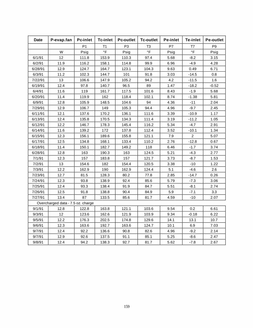
159

Date P-evap.fan Pc-inlet Tc-inlet Pc-outlet Tc-outlet Pe-inlet Te-inlet Pe-outlet

P1 T1 P3 T3 P7 T7 P9 W Psig °F Psig °F Psig °F Psig

6/1/91 12 111.8 153.9 110.3 97.4 5.68 -8.2 3.15 6/2/91 11.9 116.2 158.1 114.8 99.9 6.96 -4.9 4.28 6/28/91 12.9 124.7 164.7 123.1 104.3 9.63 0.49 6.71 6/3/91 11.2 102.3 144.7 101 91.8 3.03 -14.5 0.8 7/22/91 13 106.6 147.9 105.2 94.2 4.2 -11.5 1.6 6/19/91 12.4 97.8 140.7 96.5 89 1.47 -18.2 -0.52 6/4/91 11.6 119 161.7 117.5 101.6 8.43 -1.9 5.68 6/20/91 11.4 119.9 162 118.4 102.1 8.74 -1.38 5.81 6/9/91 12.8 105.9 148.5 104.6 94 4.36 -11 2.04 7/29/91 12.9 106.7 149 105.3 94.4 4.96 -9.7 2.45 6/11/91 12.1 137.6 170.2 136.1 111.6 3.39 -10.9 1.17 6/13/91 12.4 135.8 170.5 134.3 111.4 3.19 -11.2 1.05 6/12/91 12.2 146.7 178.3 145.4 116.2 5.34 -4.7 2.91 6/14/91 11.6 139.2 172 137.8 112.4 3.52 -10.1 1.34 6/15/91 12.3 156.1 189.6 155.8 121.1 7.9 2 5.07 6/17/91 12.5 134.8 168.1 133.4 110.2 2.76 -12.8 0.67 6/18/91 11.4 150.1 182.7 149.2 118 6.46 -1.7 3.74 6/28/91 12.8 163 190.3 163 124.5 5.21 -4.3 2.77 7/1/91 12.3 157 183.8 157 121.7 3.73 -8.7 1.53 7/2/91 13 154.6 182 154.4 120.5 3.38 -10 1.22 7/3/91 12.2 162.9 190 162.9 124.4 5.1 -4.6 2.6 7/23/91 12.7 81.5 128.3 80.2 77.8 2.85 -14.7 0.26 7/24/91 12.3 93.8 138.9 92.4 85.6 5.79 -7.3 3.06 7/25/91 12.4 93.3 138.4 91.9 84.7 5.51 -8.1 2.74 7/26/91 12.5 91.8 138.8 90.4 84.9 5.9 -7.1 3.3 7/27/91 13.4 87 133.5 85.6 81.7 4.59 -10 2.07

Overcharged data - 7.5 oz. charge 9/1/91 12.8 122.8 163.8 121.1 103.6 9.54 0.2 6.61 9/3/91 12 123.6 162.6 121.9 103.9 9.34 -0.18 6.22 9/5/91 12.2 176.3 202.5 174.8 129.6 14.1 13.1 10.7 9/6/91 12.3 163.6 192.7 163.6 124.7 10.1 6.9 7.03 9/7/91 12.4 92.2 136.6 90.8 82.6 4.96 -9.2 2.14 9/7/91 12.9 92.6 137.5 91.1 85.1 5.25 -8.6 2.47 9/8/91 12.4 94.2 138.3 92.7 81.7 5.62 -7.8 2.67

160

Date Te-outlet Psuc. Tsuc. Pcap.-inlet Tcap-inlet Tma Mdot

T9 P10 T10 P4 T4 °F Psig °F Psig °F °F lbm/hr

6/1/91 -11.1 2.87 71.1 109.3 96.6 14.715 15.17 6/2/91 25.3 3.94 78 114.3 91.6 33.563 15.999 6/28/91 24 6.38 77.8 123.1 89.9 34.102 18.433 6/3/91 -18.6 0.6 67.1 100.2 91.1 6.354 13.049 7/22/91 -16.7 1.41 60.9 104.8 93.5 5.407 14.004 6/19/91 -12.1 -0.71 68.2 96 88.3 -1.465 11.708 6/4/91 15.5 5.31 80 116.2 99.3 33.378 17.34 6/20/91 23 5.44 82.3 117.3 101.1 33.896 17.376 6/9/91 -14.7 1.79 68.3 105.6 93.3 7.992 14.227 7/29/91 -14.4 2.25 59.8 104.7 93.5 7.882 14.975 6/11/91 -14.2 1.17 86.1 135.4 110.8 8.203 12.254 6/13/91 -3.4 1.05 87.2 135.2 110.6 7.763 12.147 6/12/91 -7.2 2.88 88.3 144.6 115.4 16.382 13.767 6/14/91 3 1.34 88.5 137.3 111.6 11.133 12.333 6/15/91 25.7 4.95 98.3 154.8 120.2 34.767 15.408 6/17/91 -1.7 0.67 86.8 132.9 109.4 6.124 11.782 6/18/91 25.3 3.65 96.5 148.6 117.2 34.631 14.261 6/28/91 28.2 2.73 101.8 162.4 123.7 34.745 12.849 7/1/91 13.9 1.53 98.1 156.6 120.8 19.642 11.854 7/2/91 13.4 1.22 97.2 153.9 119.7 18.724 11.615 7/3/91 25.2 2.58 101.5 162.6 123.6 34.668 12.705 7/23/91 -20.4 -0.12 46.7 79.5 77 1.83 13.376 7/24/91 21.5 2.58 58.7 91.6 66.6 31.993 15.733 7/25/91 23.2 2.28 58.9 91.1 66.5 34.063 15.402 7/26/91 -5.9 2.84 58.7 89.9 77 15.264 16.08 7/27/91 -15 1.66 48 84.5 80.8 8.172 15.228

Overcharged data - 7.5 oz. Charge 9/1/91 19.6 6.47 80.9 120.8 97.3 29.753 18.464 9/3/91 31.1 6.1 78.7 121.9 90.5 44.028 18.123 9/5/91 10.9 10.6 100.8 173.6 128.6 43.771 20.7 9/6/91 9.2 6.98 94.9 162.9 122.5 34.637 17.447 9/7/91 30 1.81 59.2 90.4 65.8 43.352 14.895 9/7/91 22 2.14 58.7 90.7 67 32.905 15.27 9/8/91 34.2 2.34 60 92.3 66.1 51.688 15.409

161

Subcooling Subcooling Superheat Condenser Cap. Inlet Evaporator

°F °F °F -1.388 -1.159 2.856 -1.357 6.665 36.493 -1.256 13.144 29.663 -1.239 -1.023 1.577 -1.139 -0.674 1.28 -1.195 -0.806 11.908 -1.57 0.017 23.443 -1.579 -1.18 30.651 -1.292 -0.004 2.108 -1.28 -0.733 1.338 -1.892 -1.44 4.95 -2.589 -1.339 16.081 -1.98 -1.561 7.36 -1.852 -1.298 21.684 -2.059 -1.613 35.037 -1.84 -1.292 18.842 -1.993 -1.473 37.796 -2.246 -1.71 43.116 -2.117 -1.397 32.069 -2.095 -1.523 32.413 -2.19 -1.522 40.551 -0.726 -0.417 1.311 -0.378 18.11 35.682 0.202 17.888 38.193 -0.965 6.611 7.681 -0.929 -0.77 1.729

Overcharged Data - 7.5 oz. charge -1.622 4.517 25.48 -1.494 11.906 37.837 -2.283 -1.787 8.466 -2.183 -0.29 14.172 1.594 18.135 46.545 -0.712 17.13 37.686 3.714 19.058 49.371

162

R134a - Data

Date Tfreshfood Tfreshsupply Tfreshfdret Tfreezer Tfreezret Tevapfanout

°F °F °F °F °F °F

3/11/92 27.4 7.6 27.4 0.71 2.4 -2.7 3/16/92 35.7 18.9 35.6 9.8 11.7 6 3/17/92 43.1 28.6 43.1 20.4 22.2 16.3 3/18/92 50.2 37.9 50.2 30.6 32.7 26.1 3/19/92 45.9 42.2 45.8 39.1 40.8 33.7 3/20/92 53.3 52.1 53.1 50.3 52.2 45.4 2/27/92 31.1 7.5 31.1 0.5 1.9 -2.5 3/2/92 39.9 18.9 39.9 10.1 11.7 6.7 3/4/92 40.3 19.7 40.3 10.1 11.8 6.6 3/4/92 47.5 29.9 47.6 20.6 22.4 16.6 3/21/92 48.8 30.5 48.9 20.4 22.1 16.4 3/5/92 54.9 38.9 55 30.3 32.3 25.9 3/6/92 57.9 42.9 57.9 34.3 36.4 30 2/25/92 64.8 52.5 64.9 45.3 47.6 40.6 2/28/92 60.9 56.9 60.9 54.3 56.8 49.1 3/9/92 67.5 67 67.4 65.8 68.1 60.5 2/21/92 41.9 14.1 41.9 5.6 6.8 2.7 2/5/92 48.9 21.3 47.6 9.1 10.6 5.9 2/6/92 52.7 26.1 51.6 14.7 16.3 11.4 2/12/92 58.4 36.8 58.4 25.4 26.6 21.6 2/13/92 65.4 45.6 65.4 35.5 37.4 31.6 2/19/92 72.9 56 73 46.5 48.8 41.7 2/20/92 78.6 63.9 78.7 55.3 57.8 50.2 3/3/92 78.3 63.1 78.4 54.9 56.8 50.2 3/22/92 48.7 19.3 48.8 10.8 12.1 7.7 3/23/92 60.2 34.1 60.2 21.2 22.6 17.3 3/23/92 66.6 43.2 66.7 30.9 32.5 26.5 3/24/92 73.4 52.4 73.4 40.6 42.4 36.1 3/24/92 79.2 60.4 79.3 49.5 51.4 44.8 3/25/92 86.6 70.9 86.8 61 63 56.1

163

Date Tchamber Tconairin Tconfanout Qfreezer Qfreshfood P-system P-compressor

°F °F °F W W W W

3/11/92 54.4 53.5 62.9 48.2 24.8 158.8 132.5 3/16/92 54.6 53.8 63 58.9 24.8 157.6 130.6 3/17/92 54.8 54 63 65.2 24.5 155.5 128.9 3/18/92 54.1 53.5 62.5 74.1 24.8 153.7 127.7 3/19/92 54.5 53.8 62.4 94 0 150.8 124.8 3/20/92 54.6 53.9 62.3 98.8 0 148 121.6 2/27/92 69.4 68.3 78.1 34.4 24.2 164.5 139 3/2/92 69.7 68.9 78.2 44.3 24.7 164.1 137.7 3/4/92 69.5 69.8 78.2 44.9 25.3 163.4 137 3/4/92 69.5 68.9 78.2 59.1 24.8 162.5 135.4

3/21/92 69 68.3 77.5 58.1 24.9 161.2 135.6 3/5/92 69.5 68.9 78.7 68.6 24.8 161.2 135 3/6/92 69.5 68.8 78.2 71.6 24.7 160.2 134.1

2/25/92 69.3 68.5 77.8 78.7 24.7 156 130.9 2/28/92 69.4 68.6 77.6 97.2 0 154.1 129.2 3/9/92 69.4 68.8 77.5 109 0 151.6 127

2/21/92 89.6 88.6 99.1 24.9 24.8 176.9 152.9 2/5/92 89.5 88.4 98.1 24.4 24.6 170.2 146.3 2/6/92 89.5 88.4 97.9 26.2 24.1 168.1 144.4

2/12/92 89 88.2 97.7 45.9 24.6 167.9 144.6 2/13/92 89.1 88.3 97.4 50.6 24.5 165.9 142.7 2/19/92 89.2 88.5 97.4 74.1 24.3 171.2 147.8 2/20/92 89.4 88.7 98.8 81.6 24.2 169 145.6 3/3/92 89.9 89.3 98.8 74.6 24.1 167.9 142.9

3/22/92 99.3 98.4 108.7 25.2 24.9 181.2 158.4 3/23/92 99.7 98.7 108.2 36.4 24.6 180.1 156.7 3/23/92 99.5 98.6 108.7 48.4 24.4 177.7 155.1 3/24/92 99.7 98.9 108.8 58.1 24.3 177 153.6 3/24/92 99.6 98.9 108.7 65.7 24.2 174.8 151.7 3/25/92 99.5 98.8 108.5 76.1 24 172.5 149.4

164

Date P-evap.fan Pc-inlet Tc-inlet Pc-outlet Tc-outlet Pe-inlet Te-inlet

P1 T1 P3 T3 P7 T7 W Psig °F Psig °F Psig °F

3/11/92 12.9 73.8 129.1 73.3 67.1 -3.841 -27.7 3/16/92 12.8 73.7 128.8 73.7 67.3 -3.812 -27.6 3/17/92 12.6 73.1 128.1 73.1 65 -4.123 -28.7 3/18/92 12.5 72 128.3 71.9 63.8 -4.481 -30 3/19/92 12.4 71 125.5 71 63.3 -4.802 -31.2 3/20/92 12.3 70 124.7 70 61.3 -5.217 -32.8 2/27/92 12.9 98.9 144.8 97.8 82.3 -2.773 -24.1 3/2/92 12.8 98.9 144.4 98 85.2 -2.773 -24.1 3/4/92 12.8 100.8 144.2 99.9 77.3 -2.742 -24 3/4/92 12.6 100.8 144 99.9 76.3 -2.773 -24.1 3/21/92 12.6 97.4 144.1 96.6 84.4 -2.926 -24.6 3/5/92 12.5 101 143.9 100.1 75.6 -2.926 -24.6 3/6/92 12.5 100.5 143.7 99.4 73.5 -4.481 -30 2/25/92 12.4 97.7 141 96.5 75 -3.726 -27.3 2/28/92 12.3 96.3 139.8 95.3 76 -4.011 -28.3 3/9/92 12.1 96.9 139 95.9 73.2 -4.123 -28.7 2/21/92 12.9 143.4 168.6 142.3 103.2 -0.906 -18.4 2/5/92 12.8 137.7 164.9 136.6 105.4 -1.452 -20 2/6/92 12.7 135.1 165 133.9 104.3 -1.62 -20.5 2/12/92 12.5 140.2 163.5 139.1 97.4 -1.686 -20.7 2/13/92 12.4 134.5 163.3 133.4 103.9 -2.014 -21.7 2/19/92 12.3 144.5 166.2 143.5 95 -1.25 -19.4 2/20/92 12.3 143.7 165.5 142.7 94.5 -1.419 -19.9 3/3/92 12.2 140.6 164.8 139.5 104.1 -1.752 -20.9 3/22/92 12.8 164.4 180.4 163.2 116.1 -0.124 -16.2 3/23/92 12.6 165.2 179.7 164 116.2 -0.088 -16.1 3/23/92 12.5 164.9 179.3 163.8 116.1 -0.269 -16.6 3/24/92 12.4 165 179.1 163.9 115.9 -0.412 -17 3/24/92 12.3 164.4 178.2 163.1 115.6 -0.59 -17.5 3/25/92 12.2 163.2 177 162.1 115 -0.836 -18.2

165

Date Pe-outlet Te-outlet Psuc. Tsuc. Pcap.-inlet Tcap-inlet Tma

P9 T9 P10 T10 P4 T4 Psig °F Psig °F Psig °F °F

3/11/92 -6.201 -2.5 -6.651 50.3 71 55.7 4.928 3/16/92 -6.252 2.2 -6.652 51.4 71.2 56.1 14.116 3/17/92 -6.463 10.2 -7.033 52.3 70.2 55.9 24.313 3/18/92 -6.681 16 -7.081 52.5 69.1 55.5 34.469 3/19/92 -6.902 17.1 -7.282 53 68.4 55.6 41.305 3/20/92 -7.147 25.1 -7.507 53.9 67.1 55.6 52.291 2/27/92 -5.133 -1.6 -5.453 64.2 96.4 73.4 4.853 3/2/92 -5.333 4.2 -5.493 65.8 96.4 73 14.551 3/4/92 -5.152 6.7 -5.372 63.8 98 69.8 14.682 3/4/92 -5.123 14 -5.333 64.7 97.9 69.9 24.948 3/21/92 -5.306 10.8 -5.656 66.4 95.5 73.1 24.81 3/5/92 -5.146 20.9 -5.356 65.8 98.2 70.2 34.595 3/6/92 -6.691 19.5 -6.871 65.8 97.5 70 38.573 2/25/92 -5.776 30.3 -6.056 67.5 94.5 70.5 49.349 2/28/92 -5.951 34.6 -6.181 68.1 93.3 70.9 57.214 3/9/92 -6.113 43.5 -6.413 68.3 94.3 70.1 68.029 2/21/92 -3.206 4.1 -3.346 83.1 140.2 92.4 10.35 2/5/92 -3.912 5.2 -4.122 85.2 135.5 96 14.343 2/6/92 -4.02 10.4 -4.15 89.1 130.7 102.5 19.87 2/12/92 -3.946 15.5 -4.046 82.4 125.7 89.2 29.816 2/13/92 -4.184 24 -4.244 88 132 97.5 40.231 2/19/92 -3.5 33.5 -3.64 85.1 141.3 90.2 51.247 2/20/92 -3.529 38.5 -3.649 86.1 140.6 90.6 59.913 3/3/92 -3.792 35 -3.832 87.1 137.8 92.9 58.984 3/22/92 -2.284 8 -2.304 96.6 161.3 111.4 15.812 3/23/92 -2.298 15.8 -2.448 95.7 162.6 108.2 26.403 3/23/92 -2.439 22 -2.589 95.8 162.4 107 35.959 3/24/92 -2.482 28.9 -2.482 96.8 162.5 107 45.535 3/24/92 -2.6 34.7 -2.6 97.2 161.8 106.4 54.221 3/25/92 -2.756 42.4 -2.756 97.9 160.9 105.9 65.406

166

Flow Volt Mdot Subcooling Subcooling Superheat

Condenser Cap. Inlet Evaporator V lbm/hr °F °F °F

2.7396 7.574749167 4.11 13.947 34.338 2.73558 7.553656662 4.179 13.684 39.26 2.66872 7.321241241 6.076 13.196 48.18 2.62904 7.187969161 6.463 12.832 54.953 2.56951 6.976199144 6.347 12.242 57.064 2.48825 6.689417783 7.658 11.323 66.213

2.9937429 8.144909481 3.9 12.013 30.87 2.958604 8.03108987 1.112 12.413 37.456 2.910817 7.924096445 10.066 16.512 39.245 2.880265 7.81647368 11.066 16.356 46.431 2.88525 7.77628128 1.126 11.804 43.95

2.844979 7.688931096 11.876 16.223 53.422 2.775904 7.453278817 13.59 16.032 58.498 2.7683269 7.41833037 10.47 13.834 65.349 2.720745 7.246784015 8.79 12.745 70.376 2.46903 6.388971507 11.931 14.12 79.962

3.264222 8.703099093 4.861 14.742 29.626 3.1447963 8.23288978 0.145 9.051 33.152 3.1748774 8.208101817 0.027 0.363 38.731 2.887366 7.494338083 9.257 11.327 43.57 3.046514 7.8762388 0.2 5.961 52.918 3.113294 8.237783691 13.583 17.425 60.019 3.07561 8.103250821 13.735 16.718 65.119

3.044135 7.954255861 2.734 13.18 62.53 3.51624 9.153628627 0.643 4.586 30.541 3.38506 8.789124222 0.859 8.304 38.384 3.33031 8.633139747 0.88 9.425 45.029 3.29809 8.527041559 1.12 9.465 52.068 3.24834 8.374992975 1.103 9.786 58.244 3.18216 8.166544511 1.305 9.926 66.446

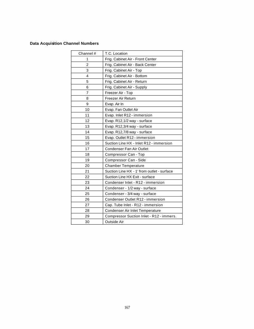
167

Data Acquisition Channel Numbers

Channel # T.C. Location 1 Frig. Cabinet Air - Front Center 2 Frig. Cabinet Air - Back Center 3 Frig. Cabinet Air - Top 4 Frig. Cabinet Air - Bottom 5 Frig. Cabinet Air - Return 6 Frig. Cabinet Air - Supply 7 Freezer Air - Top 8 Freezer Air Return 9 Evap. Air In

10 Evap. Fan Outlet Air 11 Evap. Inlet R12 - immersion 12 Evap. R12,1/2 way - surface 13 Evap. R12,3/4 way - surface 14 Evap. R12,7/8 way - surface 15 Evap. Outlet R12 - immersion 16 Suction Line HX - Inlet R12 - immersion 17 Condenser Fan Air Outlet 18 Compressor Can - Top 19 Compressor Can - Side 20 Chamber Temperature 21 Suction Line HX - 1' from outlet - surface 22 Suction Line HX Exit - surface 23 Condenser Inlet - R12 - immersion 24 Condenser - 1/2 way - surface 25 Condenser - 3/4 way - surface 26 Condenser Outlet R12 - immersion 27 Cap. Tube Inlet - R12 - immersion 28 Condenser Air Inlet Temperature 29 Compressor Suction Inlet - R12 - immers. 30 Outside Air

168

Appendix G: Film Coefficients

G.1 Condenser Film Coefficients The air side film coefficient for the condenser was estimated from Equation G.1 which is the correlation by

Hilpert [1] for a cylinder in crossflow. Evaluating this expression for the nominal conditions listed results in an air side

convective film coefficient of 14.0 Btu/hr-ft2°F

NuD__

= 0.683 ReD

0.466 Pr0.33 (G.1)

where ReD = 838 (based on condenser inlet area of 40 in2)

D = 0.25 in

Pr = 0.713

Tair = 80°F

The internal film coefficients must be determined from convective heat transfer correlations. For the

desuperheating section, the Dittus-Boelter equation given by Equation G.2 was used [2]. For the R134a subcooled

section, the maximum calculated Reynolds number is 1500, well below the transition Reynolds number to turbulent

flow. The theoretical expression for laminar flow with constant heat flux given by Equation G.3 was used for the

subcooled section [3].

hdesup = 0.023Re0.8Pr0.3

D

k supde (G.2)

hsub = 4.36

D

k sub (G.3)

The film coefficient for the two phase section is more complicated. The correlation by Cavallini-Zecchin [4]

was chosen and is given by Equation G.4. The two phase film coefficient in this correlation is a function of quality.

Since the quality in the two phase section of the condenser varies from one to zero, the film coefficient must also

vary. To simplify the model an average value was determined by integrating. For reference Figure G-1 shows the

variation in the film coefficient for typical data points for both the R12 and R134a cases. Note that the film coefficient

for the R12 case is higher than the R134a case because the Reynolds number for the R12 data point is higher.

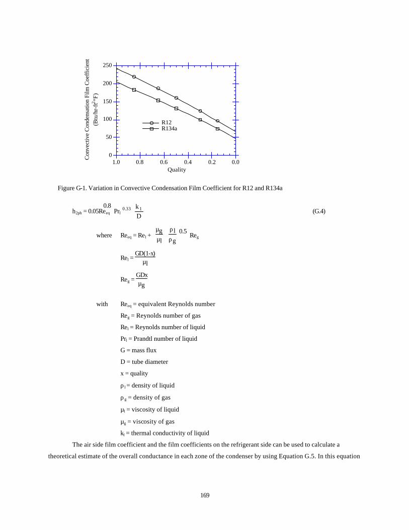
169

0

50

100

150

200

250

Con

vect

ive

Con

dens

atio

n Fi

lm C

oeff

icie

nt(B

tu/h

r-ft2 °F

)

1.0 0.8 0.6 0.4 0.2 0.0Quality

R12R134a

Figure G-1. Variation in Convective Condensation Film Coefficient for R12 and R134a

h2ph = 0.05Reeq

0.8 Prl

Dk133.0 (G.4)

where Reeq = Rel +

µg

µl

ρl

ρg0.5

Reg

Rel = GD(1-x)

µl

Reg = GDxµg

with Reeq = equivalent Reynolds number

Reg = Reynolds number of gas

Rel = Reynolds number of liquid

Prl = Prandtl number of liquid

G = mass flux

D = tube diameter

x = quality

ρ l = density of liquid

ρg = density of gas

µl = viscosity of liquid

µg = viscosity of gas

kl = thermal conductivity of liquid

The air side film coefficient and the film coefficients on the refrigerant side can be used to calculate a

theoretical estimate of the overall conductance in each zone of the condenser by using Equation G.5. In this equation

170

the wall resistance has been neglected. However, because the condenser does have wire fins, the fin effectiveness is

accounted for.

i

ix

oo

ox

x hA/A

hA/A

U1

+η

= (G.5)

where ηo = fin effectiveness

Ax = outside surface area of the condenser tubing in either section

Ao = total outside surface area - includes wire fins

Ai = inside surface area of the condenser tubing

ho = air side convective film coefficient

hi = refrigerant side convective film coefficient for either section

The fin effectiveness is determined from Equation G.6 where the fin efficiency is given by Equation G.7. Note

that the fin effectiveness is for a pin fin and it is assumed that this closely approximates the wire fins in the

condenser. A summary of the fin effectiveness calculations is given in Table G.1

)1(AA

1 fo

fo η−−=η (G.6)

where Af = fin surface area (ft2)

Ao = total outside surface area (ft2)

mL)mLtanh(

f =η (G.7)

where m2 = 4hspine

kd

hspine = film coefficient for spine fin (Btu/hr-ft2°F)

k = thermal conductivity of fin material (Btu/hr-ft°F)

d = spine diameter (ft)

L = spine length

Table G.1. Condenser Fin Effectiveness Calculation Results

dwire 0.0625 in. L/tube 0.625 in hspine 10.2 Btu/hr-ft2°F

m 15.0/ft ηf 0.836

Wire spacing 3.5 wires/in. Af 0.01193 ft2/in

Atube 0.00545 ft2/in Af/Ao 0.686 ηo 0.888

171

The results of solving Equation G.5 for all the data points in both the R12 and R134a data sets are

summarized in Table G.2. The last row shows the ranges of the theoretical conductances for the variation in the

internal film coefficients.

Table G.2. Theoretical Condenser Conductances

R12 R134a

Condenser Section

Desuperheating Section

Two Phase

Section

Desuperheating Section

Two Phase

Section

Subcooled Section

ho (Btu/hr-ft2°F)

10.2 10.2 10.2 10.2 10.2

Minimum h i

(Btu/hr-ft2°F) 25.8 119.8 23.6 115.3 9.9

Maximum h i (Btu/hr-ft2°F)

44.2 190.2 34.9 141.7 11.6

Average h i (Btu/hr-ft2°F)

32.0 160.9 29.0 129.8 10.7

Ax/Ao 0.31 0.31 0.31 0.31 0.31

Ax/Ai 1.14 1.14 1.14 1.14 1.14

ηo 0.89 0.89 0.89 0.89 0.89

Conductances (Btu/hr-ft2°F)

12.8 - 16.7 22.9 - 24.9

12.1 - 15.0 22.7 - 23.7

6.7 - 7.6

G.2 Evaporator Film Coefficients The calculation of the evaporator film coefficients is very similar to the condenser except for the two phase

film coefficient. As for the condenser the correlation by Hilpert [1] was used to calculate the air side film coefficient.

Equation G.1 is repeated here as Equation G.8 with the conditions used in the equation listed. The outside film

coefficient was found to be 7.1 Btu/hr-ft2°F. Further for the superheated section film coefficient, the Dittus-Boelter

correlation given by Equation G.2 was used except the Prandtl number is raised to the 0.4 power.

NuD__

= 0.683 ReD

0.466 Pr

0.33 (G.8)

where ReD = 795 (based on evaporator inlet area of 36 in2)

D = 0.3125 in.

Pr = 0.72

Tair = 8°F

The two phase film coefficient was determined from the correlation by Kandlikar given by Equation G.9. This

correlation was chosen to calculate the two phase film coefficients because it is based on a large data set for 10 fluids

[4].

htphl

= c1Coc2

(25Frl)c5

+ c3Boc4

Ffl (G.9)

hl = 0.023Rel0.8Prl

0.4

kl

D

172

Rel = GD(1-x)

µ

Where htp = two phase film coefficient

hl = film coefficient for liquid

Rel = Reynolds for liquid

Prl = Prandtl for liquid

kl = thermal conductivity for liquid

Co = convection number

Frl = Froude number for liquid

Bo = boiling number

Ffl = fluid specific parameter

c1,c2, etc. = constants - see reference

G = mass flux

x = refrigerant quality

Since the Reynolds number is a function of quality, the film coefficient varies not only as a function of fluid

properties but also with quality. An average film coefficient was determined by integrating over the typical quality

range for the evaporator. For reference, Figure G-2 shows the variation in two phase film coefficient with quality for

typical R12 and R134a data points.

0

100

200

300

400

500

600

Two

Phas

e Ev

apor

atin

g Fi

lm C

oeff

icie

nt(B

tu/h

r-ft2 °F

)

700

0.3 0.4 0.5 0.6 0.7 0.8 0.9 1.0Quality

R12R134a

Figure G-2. Variation in Two Phase Film Coefficients with Quality

Using the estimates of the air side and refrigerant side film coefficients it is also possible to use Equation G.5

to estimate theoretical conductances for the evaporator. The evaporator instead of wire fins has spine fins. As a

result, the fin effectiveness of the spines is considered. The same equations given by Equations G.6 and G.7 were

also used for the evaporator. The fin effectiveness calculations for the evaporator are summarized in Table G.3. The

results of solving Equation G.5 for each zone in the evaporator is given in Table G.4.

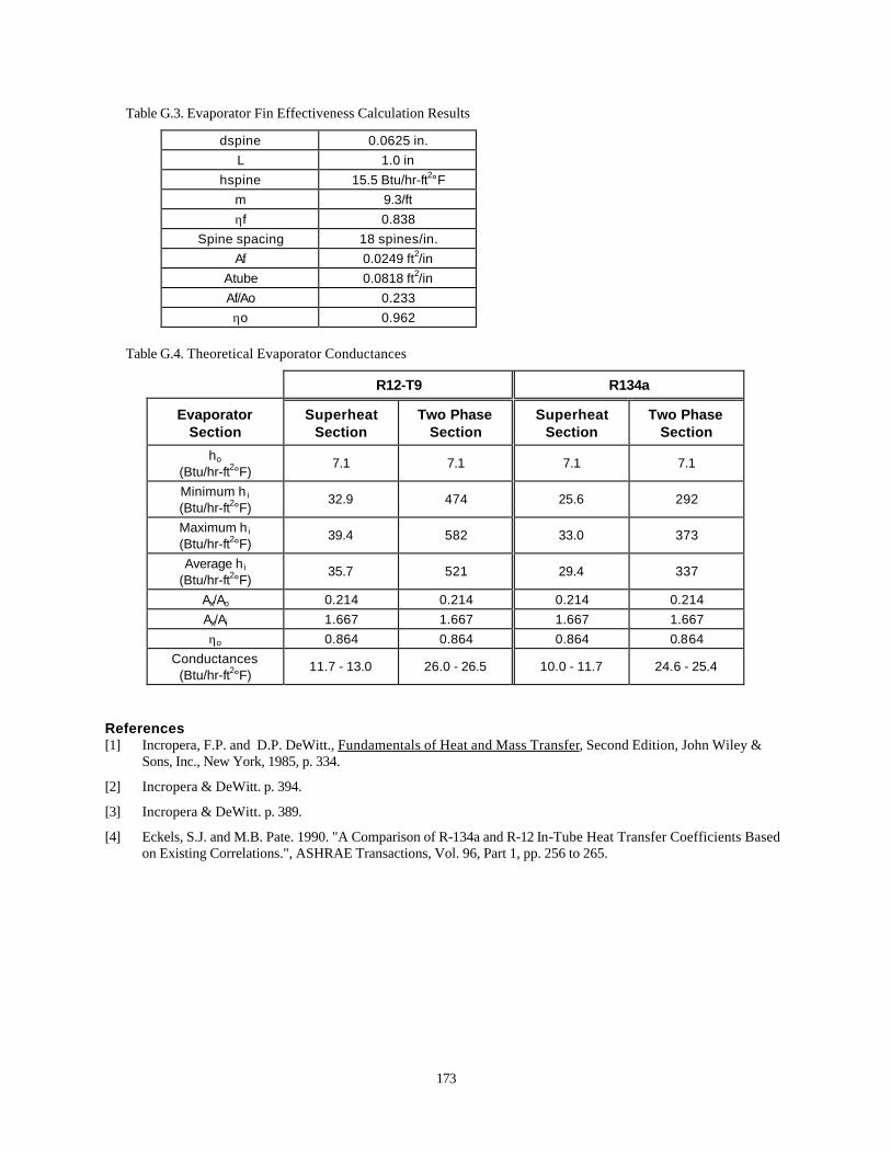
173

Table G.3. Evaporator Fin Effectiveness Calculation Results

dspine 0.0625 in. L 1.0 in

hspine 15.5 Btu/hr-ft2°F m 9.3/ft ηf 0.838

Spine spacing 18 spines/in. Af 0.0249 ft2/in

Atube 0.0818 ft2/in Af/Ao 0.233 ηo 0.962

Table G.4. Theoretical Evaporator Conductances

R12-T9 R134a

Evaporator Section

Superheat Section

Two Phase Section

Superheat Section

Two Phase Section

ho (Btu/hr-ft2°F)

7.1 7.1 7.1 7.1

Minimum h i

(Btu/hr-ft2°F) 32.9 474 25.6 292

Maximum h i (Btu/hr-ft2°F)

39.4 582 33.0 373

Average h i (Btu/hr-ft2°F)

35.7 521 29.4 337

Ax/Ao 0.214 0.214 0.214 0.214 Ax/Ai 1.667 1.667 1.667 1.667 ηo 0.864 0.864 0.864 0.864

Conductances (Btu/hr-ft2°F)

11.7 - 13.0 26.0 - 26.5 10.0 - 11.7 24.6 - 25.4

References [1] Incropera, F.P. and D.P. DeWitt., Fundamentals of Heat and Mass Transfer, Second Edition, John Wiley &

Sons, Inc., New York, 1985, p. 334.

[2] Incropera & DeWitt. p. 394.

[3] Incropera & DeWitt. p. 389.

[4] Eckels, S.J. and M.B. Pate. 1990. "A Comparison of R-134a and R-12 In-Tube Heat Transfer Coefficients Based on Existing Correlations.", ASHRAE Transactions, Vol. 96, Part 1, pp. 256 to 265.