status of the longitudinal emittance preservation at the...
TRANSCRIPT

Status of theLongitudinal Emittance Preservation
at the HERA Proton Ringin Spring 2003
Elmar VogelDeutsches Elektronen-Synchrotron DESY, Hamburg, Germany
DESY Report No. DESY-HERA-03-03, 2003

ii

Abstract
At the upgraded electron proton collider HERA (HERA II), the proton bunch length is relevantfor the achievable luminosity. This is due to the enhancement of the effective cross section atthe interaction region when the beta function and the bunch length have comparable magnitude,‘hour-glass-effect’ [1].Several beam dynamical effects, such as beam loading transients at injection, coupled bunch
oscillations during ramping and technical problems lead to a longitudinal emittance dilution.These effects can now be routinely observed and are permanently recorded with the new fastlongitudinal diagnostics system (FLD). To reduce the bunch length, we began to implementseveral measures, such as RF amplitude modulation, introducing Landau damping at low energyand debugging the frequency controls and RF systems. In this report, the actual status of theseactivities will be given.
iii

iv Abstract

Contents
1 Introduction 1
2 Data Acquisition and Archiving 32.1 Measured Values . . . . . . . . . . . . . . . . . . . . . . . . . . . . . . . . . 32.2 Front End Computer . . . . . . . . . . . . . . . . . . . . . . . . . . . . . . . 32.3 Data Archiving . . . . . . . . . . . . . . . . . . . . . . . . . . . . . . . . . . 42.4 Data Representation . . . . . . . . . . . . . . . . . . . . . . . . . . . . . . . . 5
3 Observed Emittance Dilution Effects 93.1 Injections . . . . . . . . . . . . . . . . . . . . . . . . . . . . . . . . . . . . . 93.2 Low Energy and Ramp up to 70 GeV . . . . . . . . . . . . . . . . . . . . . . . 123.3 Coupled Bunch Oscillations above 70 GeV . . . . . . . . . . . . . . . . . . . 173.4 RF Noise Effects . . . . . . . . . . . . . . . . . . . . . . . . . . . . . . . . . 20
4 Tested Measures for Emittance Preservation 234.1 The Use of the Phase Loops . . . . . . . . . . . . . . . . . . . . . . . . . . . 234.2 RF Setting at Low Energy for Landau Damping . . . . . . . . . . . . . . . . . 264.3 RF Amplitude Modulation . . . . . . . . . . . . . . . . . . . . . . . . . . . . 29
4.3.1 Using a h+ 1 cavity . . . . . . . . . . . . . . . . . . . . . . . . . . . 294.3.2 Direct RF amplitude modulation . . . . . . . . . . . . . . . . . . . . . 304.3.3 Experiences made with the direct RF amplitude modulation . . . . . . 334.3.4 Actual limits of the direct RF amplitude modulation . . . . . . . . . . 38
4.4 RF Setting at High Energy . . . . . . . . . . . . . . . . . . . . . . . . . . . . 38
5 Continue Fighting the Blow Up 415.1 Further Debugging HERA Longitudinally . . . . . . . . . . . . . . . . . . . . 415.2 Examinations of new RF Voltage Ramp-Tables . . . . . . . . . . . . . . . . . 415.3 Amplitude-Modulation as a Standard Device . . . . . . . . . . . . . . . . . . . 425.4 Further Development of the FLD . . . . . . . . . . . . . . . . . . . . . . . . . 435.5 Further Measures . . . . . . . . . . . . . . . . . . . . . . . . . . . . . . . . . 44
6 Conclusion 45
Appendix 47A.1 Amplitude Modulation due to h+ 1 Cavity . . . . . . . . . . . . . . . . . . . 47A.2 Direct RF Amplitude Modulation . . . . . . . . . . . . . . . . . . . . . . . . . 48
Bibliography 50
Acknowledgments 53
v

vi Contents

1 Introduction
At HERA II, strong focussing, superconducting magnets inside the detectors H1 and ZEUS leadto smaller beam cross sections at the interaction regions and hence to higher luminosity. Due tothe strong focussing, the beta function and the bunch length are comparable in magnitude. Thisenhances the effective cross section, ‘hour-glass-effect’ [1]. A reduction of the bunch lengthwould result in smaller effective cross sections and so further increase the luminosity.
0.08 0.12 0.180.06 0.10 0.14 0.16
1.5
1.4
1.3
1.2
1.1
1.0
lum
inos
ity g
ain
vertical proton -function in m�
ns0.2�FWHMl
ns8.1�FWHMl
ns6.1�FWHMl
ns4.1�FWHMl
maximumluminosity
curve
ns2.1�FWHMlns0.1�FWHMl
ns8.0�FWHMl
ns6.0�FWHMl
design working point
ns1273.0
mFWHMs l
�
�
Figure 1.1: Dependence of the HERA II luminosity gain on the vertical proton β-function andthe bunch length. (Ldesign ≈ 7 · 1031 1
cm2 s )
Figure 1.1 shows the luminosity gain, scaled from the design value, as a function of thevertical proton β-function and the bunch length1. The geometrical aperture of the proton storagering, especially in the half quadrupole magnets with mirror plates, gives a lower limit for thevertical proton β-function. For commissioning 18 cm was chosen to have enough safety margin.The safety margin from the last HERA operation period, using the old optics, allow 12 cm. Afurther reduction is a challenge, the lowest possible limit seems to be 8 cm [2].Typical FWHM bunch lengths after injection (40GeV) into 52 MHz buckets are between
2.4 ns and 3.5 ns. Bunch lengths at low energy above 2.4 ns are caused by beam loading tran-sients during injections and beam oscillations which could be driven by the 52MHz RF cavities,or by their control loops. During acceleration to 920 GeV, the bunch length reduces to 1.6 nsdue to mainly the compression by an additional 208 MHz RF system. One would theoretically
1Here we quote bunch length in the time domain.
1

2 Introduction
expect a bunch length of l920 GeV ≈ 0.27 l40 GeV i.e. ≈ 0.6 ns at high energy from a bunch lengthof 2.4 ns at low energy. This is mainly prevented by coupled bunch oscillations during the ramp.With the new Fast Longitudinal Diagnostic (FLD) system we are able to observe and record
all these effects. Furthermore we have an on-line check, whether particular measures suppressthem and whether they are sufficient to preserve the longitudinal emittance. In this report,the observed and examined emittance dilution effects at injection and during acceleration arepresented and the actual status of the measures taken is discussed.High energy protons stored in HERA, which are not trapped in the RF buckets are called
‘coasting beam’. This beam complicates the data taking at experiments examining low anglescattering, such as the Very Forward Proton Spectrometer (VFPS) of H1, or the using the beamhalo for collisions with a fixed target, HERA-B. Systematic examination of coasting beam pro-duction at high energy and measures to reduce the production rate are at an initial stage. Somefirst results are presented.

2 Data Acquisition and Archiving
In this chapter, the current features of the Fast Longitudinal Diagnostics (FLD) are presentedfrom the view of a user. The underlying principles have been described in detail in [3]. Incontrast to the previous work, the recent period of development was dominated by softwaredevelopment to integrate the system as a standard tool into the HERA control system and tomake it comfortable and easy to use. The sophisticated data acquisition and archiving softwarewas written by Hong Gong Wu1, whereas Victor Soloviev2 developed the comfortable displayprogram.
2.1 Measured ValuesAt the Fast Longitudinal Diagnostics System (FLD) the expression ‘Fast’ means that the phase,length and intensity of each single bunch are recorded within the time subsequent bunches passa resistive gap monitor. In practice, this is equivalent to a simultaneous recording of theseparameters from all proton bunches in HERA. Furthermore, the system records RF transients inall six cavities. These transients are built up by the beam loading and the RF fast feedback loops,installed to suppress the beam loading. Accelerating cavity voltages and the phasing betweenthe two RF frequencies of the proton ring, 52 MHz and 208 MHz, complete the measured data.On account of the limited memory size on the ADC boards, the raw data is recorded for a
certain time period before reading the memory out. After preprocessing this data, it is storedon a local hard disc. By setting particular parameters in the FLD timing hardware, the timeperiod can be adjusted in steps between 0.14 seconds and 4.5 seconds. This corresponds tothe different sampling rates of single bucket positions every 13th, 26th, 52th, 104th, 208th and416th revolution. One record requires 4 Mbyte. All calibration and conversion factors used arealso stored, in order to have the possibility of re-calibrating the data for later off line analysis.In addition, each record contains so called ‘global variables’, such as the accelerator energy,DC-current, status of phase loops and the longitudinal profile of a single bunch (‘CMFL’ or‘Lopez Monitor’ at DESY).The calculation power of the VME CPU used allows one record to be taken every 11 sec-
onds. During injection, acceleration and one hour after high energy is reached, the system takesrecords within this interval. Afterwards, the time intervals are increased to 3 minutes and 40seconds. Without beam, the data recording is stopped.
2.2 Front End ComputerA ‘Front End Computer’ (FEC) is a data acquisition computer which acquires and preprocessesraw data, taken from diagnostics hardware. The software processing this data at a FEC is called‘server’. A server also places the data at the users disposal, whereas the access takes placeover the network. Display programs are running at the consoles in the accelerator control room(BKR) and selected computers in the laboratory offices. The software layer between them and
1from DESY group MST2from DESY groups MPY respectively MST
3

4 Data Acquisition and Archiving
the servers is at HERA the TINE (Three-fold Integrated Network Environment) protocol [4].The whole software containing the servers the display programs and the layers between is called‘control system’.In the case of the FLD the FEC consists of an industry standard VME crate containing an
AMD CPU with 330 MHz and a local IDE hard disc with about 30 Gbyte of capacity for in-termediate data storage. Hard discs according to the IDE standard are not optimal, since ouraverage data throughput is about 30 Gbyte in four days and we operate 24 hours per day. Wealready crashed hard discs. The use of hard discs according to the SCSI standard is in prepa-ration. After testing several operating systems, the actual one used is the LINUX distributionDebian 3.0.The raw data is sampled by five VME ADC boards each containing eight ADC channels,
with a digital bandwidth of 10.6 MHz and an analog bandwidth of about 60 MHz. The boardsused have been developed by DESY-ZEUTHEN for use at the Tesla Test Facility (TTF) andits successors [5]. Four ADC boards are used for the FLD standard data acquisition mode andone is installed for long time observations of single bunches as needed for high sensitive beamspectrum and beam echo measurements.To supply the ADC board with clock and trigger signals with low jitter, the FLD also con-
tains a ‘timing’-crate, developed by the DESY group FEA. In this unit, ECL gate arrays count208 MHz RF waves to generate among others bunch clock signals. Several FPGA (field pro-grammable gate array) units provides trigger signals by counting the clock signals. Delay linesallow the clock signals to be shifted for each ADC board in steps of 500 ps independently. Onecan remotely switch and control the timing modules via IO interfaces. For this purpose a VMEIP-Digital carrier board from Green Spring Computers is installed, equipped with IP-DigitalI/O IndustryPacks.A tolerable access time to the data is guaranteed by an exclusive 100 Mbit/s network con-
nection to the next router in the computer network.
2.3 Data ArchivingThe ADC boards cause interrupt requests on the VME bus when a data record has been taken.This forces the data acquisition server to fetch the raw data, preprocess it and store it on thehard disc. Display programs only access this data record via a second server, called ‘archiveserver’. In this way, the data acquisition can not be disturbed by an increasing demand fromdisplay programs.Two chron-jobs are running at the FEC. One prevents overrun of the local hard disc by
deleting the oldest records when the disc is 90% full. The other combines together data recordsin packages of about 300 Mbyte as zip-files. These packages are copied to the DESY tapesystem ‘dCache’ [6] to give a durable archive. Our philosophy is to store as much data aspossible to allow off line analysis without restrictions. Such restrictions are always caused bya preliminary selection of events for storage. We need more memory, but it turned out, that weare therefore able to examine successfully malfunctions occurring at HERA only once or twicea week during standard operation.While the FEC is taking a data record every 11 seconds, the CPU has no time to generate
zip-files in parallel. Therefore, the chron-job for storing data at the dCache first checks thestatus of the data acquisition server and only takes action when the server is acquiring data inlarger time intervals or is idle.Data records already deleted at the FEC but stored at the dCache can be obtained from
a second archive server also running on a LINUX PC called ‘archive PC’. In addition to thearchive server on the FEC, this server checks whether a particular record is actually stored on

2.4 Data Representation 5
the archive PCs hard disc in case there is an request for it. If the record is not available, the datapackage containing it, is copied back from the dCache, unzipped and the record supplied to therequesting user. This server is still under construction.The archive PC also has an exclusive 100 Mbit/s network connection to the next router for
tolerable access times.
2.4 Data RepresentationFor data representation in the control room and the laboratories offices, a comfortable displayprogram was developed. It has two operation modes, figure 2.1. In the live mode it always
Figure 2.1: The FLD main window for the two different operation modes, the live mode and thearchive mode. In the archive mode the window shows a calendar for choosing the time intervalone is interested in.
Figure 2.2: At the moment, 30 displays for the presentation and analysis of different aspects ofa dada record are realized.
6 Data Acquisition and Archiving
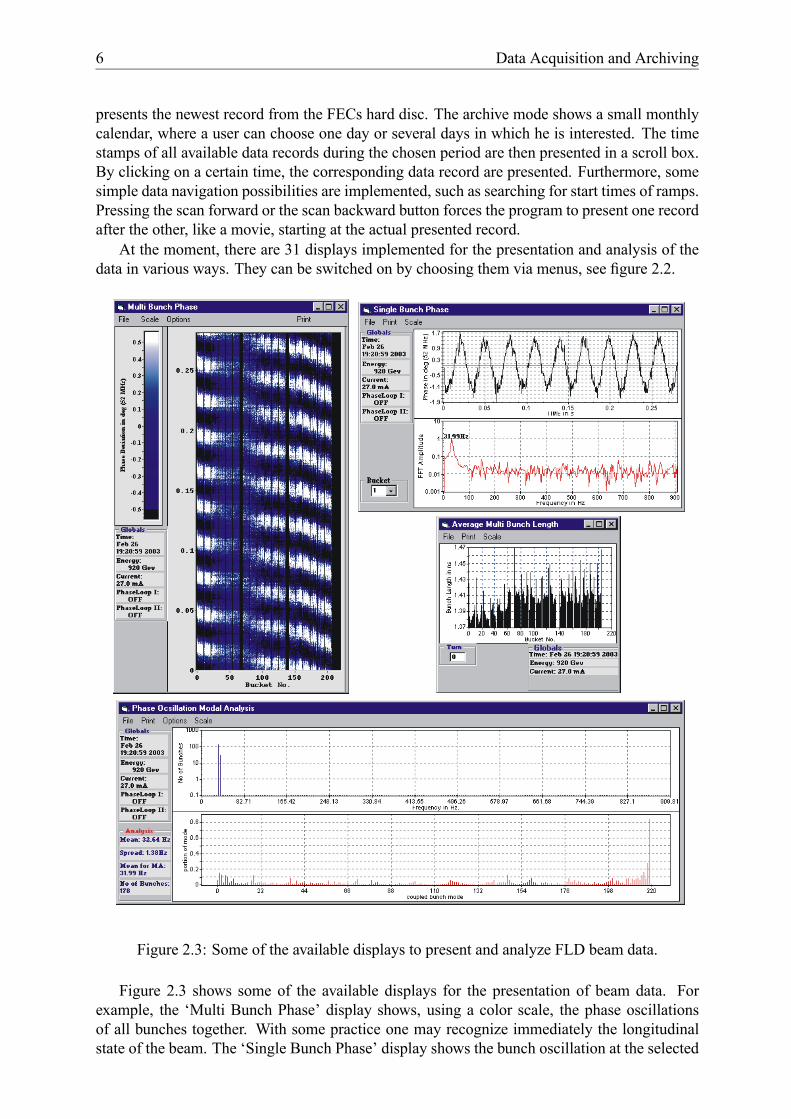
presents the newest record from the FECs hard disc. The archive mode shows a small monthlycalendar, where a user can choose one day or several days in which he is interested. The timestamps of all available data records during the chosen period are then presented in a scroll box.By clicking on a certain time, the corresponding data record are presented. Furthermore, somesimple data navigation possibilities are implemented, such as searching for start times of ramps.Pressing the scan forward or the scan backward button forces the program to present one recordafter the other, like a movie, starting at the actual presented record.At the moment, there are 31 displays implemented for the presentation and analysis of the
data in various ways. They can be switched on by choosing them via menus, see figure 2.2.
Figure 2.3: Some of the available displays to present and analyze FLD beam data.
Figure 2.3 shows some of the available displays for the presentation of beam data. Forexample, the ‘Multi Bunch Phase’ display shows, using a color scale, the phase oscillationsof all bunches together. With some practice one may recognize immediately the longitudinalstate of the beam. The ‘Single Bunch Phase’ display shows the bunch oscillation at the selected

2.4 Data Representation 7
bucket together with the FFT of this oscillation. The result of the steady state coupled bunchmodal analysis, described in [3], is presented in the ‘Phase Oscillation Modal Analysis’ display.‘Average’ displays are available for the presentation of the mean values of bunch phases, lengthand intensities. The values are calculated by averaging all values, contained in a data record,for each bucket position separately.Figure 2.4 shows some displays for the presentation of cavity data. In the ‘Average Cavity
Figure 2.4: Displays to present and analyze cavity data.
Transient’ display, the average steady state between beam loading and its suppression due to thefast feedback loops is presented. The ‘Cavity Transient’ display show the deviation from thisaverage for the time at which the data record was taken. With the ‘Transient at Bucket’ displays,one can select one bucket position to examine the deviation from the average voltage a bunch atthis position will see. A polar plot of the cavity voltages time averaged over all buckets is givenin the ‘52 & 208 MHz Cavity Voltage’ display.We will not discuss here all features of the displays with respect to the different scaling

8 Data Acquisition and Archiving
possibilities such as auto-scale, fixed scale, linear and logarithmic for FFT and so forth. Alot of these features should be self-explanatory. Choosing the print menu a user can send thedisplay to a printer or even to the electronic HERA logbook.For off line analysis, we also implemented the possibility to export the data, actually pre-
sented in a display, as a csv-file. Standard spread sheet programs import such files directly.Figure 2.5 shows this possibility using the ‘Bunch Charge’ display.
Figure 2.5: Choosing ‘Export Data’ in the ‘File’ menu opens a ‘Save As’ dialog box to changethe recommend file name and path. The exported data is stored as a csv-file.
The FLD display program supports the user in post mortem analysis. He has only to switchthe program into archive mode. Development of the display program is also uncoupled from ac-celerator operation. One can develop new displays even during shutdown periods by accessingarchived data.

3 Observed Emittance Dilution Effects
In this chapter, we will discuss the most prominent emittance dilution effects, observed at theHERA proton ring. After suppressing these effects, additional effects may come to light. Theyare not yet considered.
3.1 InjectionsThe preservation of the longitudinal proton bunch emittance during the transfer from the pre-accelerator PETRA to HERA require the so called bunch rotation. The expression ‘rotation’means that the bunch distribution is rotated in the PETRA phase space before the transfer,to match with the HERA buckets. This is done by changing every quarter synchrotron cyclethe amplitude of the PETRA RF in steps. After each voltage change, the bunch rotates evenmore in phase space, observed as bunch length oscillation. But, this also dilutes the emittance.The optimum timing for transferring short bunches with low emittance is after three quartersynchrotron oscillations. The whole process is adjusted to result in matched bunch distributionsin the HERA buckets [7].As long as one transfers only one bunch from PETRA to HERA the bunch rotation results,
in principle, in an ideal bucket matching. If there are already bunches inside HERA, eitherprevious ones from an actual transferred train or from already stored bunch trains, they modifysubsequent bucket potentials by beam loading. For subsequent bunches the bucket matching isno longer ideal, resulting in bunch oscillations and an increase of the longitudinal emittance.Furthermore, new injected bunches also cause beam loading acting on already stored bunches.All these transient effects together lead to an increase of the longitudinal emittance.
69
70
71
0.0 0.5 1.0 1.5 2.0
-1
0
1
2
3
volta
ge o
f 52
MH
zca
vity
B a
t buc
ket
no 9
3 in
kV
time in sec
phas
e ch
ange
in52
MH
z ca
vity
Bat
buc
ket 9
3 in
deg
Figure 3.1: Transient changes of the RF in the 52 MHz cavity B due to the injection of the thirdbunch train (24th February 2003 at 00:08:10).
Figures 3.1 to 3.3 show the effect of the injection of 23 mA protons in a train of 40 bunchesinto HERA, when 45 mA in 80 bunches are already stored. The figures show the changes at
9

10 Observed Emittance Dilution Effects
the arbitrary chosen bucket position no 93. Figure 3.1 and 3.2 present the transient changes ofthe RF voltages in the second 52 MHz cavity and the first 208 MHz cavity. The other cavitiesbehave similary. The RF transients shown cause a phase oscillation of the bunch at position 93resulting in a bunch lengthening and a loss of intensity, as shown in figure 3.3.Aside, the particular fill pattern of three times 40 bunches was used to check, whether one
can reach higher integrated luminosity with lower background in the experiments H1 and ZEUSas compared to the normal fill pattern of tree times 60 bunches. This divergence from the normaloperation makes no fundamental difference in view of the beam loading effects shown.
9698
100102104106
0.0 0.5 1.0 1.5 2.0
-2-1012345
volta
ge o
f 208
MH
zca
vity
A a
t buc
ket
no 9
3 in
kV
time in sec
phas
e ch
ange
in20
8 M
Hz
cavi
ty A
at b
ucke
t 93
in d
eg
Figure 3.2: Transient changes of the RF in the 208 MHz cavity A due to the injection of thethird bunch train.
-8
-4
0
4
8
2.5
3.0
3.5
4.0
0.0 0.5 1.0 1.5 2.0
6.36.46.56.66.7
bunc
h ph
ase
(no.
93)
in d
eg (5
2 M
Hz)
bunc
h le
ngth
in n
s
time in sec
bunc
h in
tens
ityin
1010
par
ticle
s
Figure 3.3: Oscillation of the already stored bunch at position 93, increase of its length and theloss of intensity due to the injection of the third bunch train.

3.1 Injections 11
2.4
2.8
3.2
3.6
2.4
2.8
3.2
3.6
0 20 40 60 80 100 120 140 160 180 200 220
2.4
2.8
3.2
3.6
bu
nch
leng
thin
ns
first
trai
n
bu
nch
leng
thin
ns
two
train
s
bucket number
bunc
h le
ngth
in n
sth
ree
train
s
Figure 3.4: Bunch length development due to transient beam loading, caused by subsequentinjected trains of 40 bunches each. The beam current after the last injection was 69 mA. Datafrom 24th February 2003 starting at 00:00 AM.
2.2
2.4
2.6
2.2
2.4
2.6
0 20 40 60 80 100 120 140 160 180 200 220
2.2
2.4
2.6
bunc
h le
ngth
in n
sfir
st tr
ain
bunc
h le
ngth
in n
stw
o tra
ins
bucket number
bunc
h le
ngth
in n
sth
ree
train
s
Figure 3.5: Bunch length development due to transient beam loading, caused by subsequentinjected trains of 60 bunches each. The beam current after the last injection was 32 mA. Datafrom 16th January 2003 starting at 01:20 AM.

12 Observed Emittance Dilution Effects
The bunch lengthening during the subsequent injection of three trains, each containing 40bunches, is shown in figure 3.4. Figure 3.5 shows the case when trains of 60 bunches areinjected.Long bunches at the start of the acceleration normally lead to side-bunches in the neighbor-
ing 208 MHz buckets at high energy, this mean at the positions ±5 ns from the bunch center.This is due to the bunch being too long for a proper transition from the initial 52 MHz potentialinto the 208 MHz potential. An extreme example is shown in figure 3.6, where a bunch withan initial length of 4.7 ns at low energy forms neighboring bunches during acceleration to highenergy. The bunch length of 4.7 ns corresponds to a longitudinal emittance of 190meVs at lowenergy.
0 5 10 15 20
0
2
4
6
0 5 10 15 20
0
2
4
6bucket no. 5at 40 GeV
sam
pled
sig
nal
(arb
itrar
y un
its)
time in ns
bucket no. 5at 920 GeV
sam
pled
sig
nal
time in ns
Figure 3.6: CMFL trace of a 4.7 ns long bunch at 40 GeV. Its length is reduced to 1.7 ns at920GeV. But, 5 ns in front of it, an additional bunch was formed (23. February 2003 02:02 PM).
Side-bunches seriously interfere with the data taking in the experiments H1, ZEUS andHERA-B.
3.2 Low Energy and Ramp up to 70 GeVDuring the last HERA run period, we observed strong coherent beam oscillations at low energywith coupled bunch mode number l = 0. This means, all bunches oscillated in phase as figures3.7 and 3.8 show. Reaching 70 GeV, these oscillations disappeared.In May 2002, such oscillations were not visible, unfortunately we no longer have stored
FLD data from this time since the FLD was still in an early development state. Nevertheless,even older data from HERA before the upgrade (HERA I), taken in 2000 with a test software,also shows no comparable oscillations, even with four times higher beam current, figure 3.9.Already at the time of the first observation of these oscillations in July 2002, we had the sus-
picion that a technical malfunction in the 52 MHz part of the proton RF system was responsiblefor this effect. The reason for this suspicion was the disappearance of the oscillations at energiesof 70 GeV. At this energy, the 208 MHz system starts to take over the provision of the bucketsfrom the 52MHz system. This transition is completed at 150 GeV. But even at the start of thisprocess, the bucket potential becomes more non-parabolic and thus increases Landau dampingwhich damps oscillations. In the case of a malfunction in the 208 MHz system, we expect toobserve such oscillations also at higher energies, when the buckets are mainly provided by the208MHz RF system.Surprisingly, all standard parameters from the proton RF controls showed normal values
and the storage rings operation was not further interfered. Measurements with respect to RF

3.2 Low Energy and Ramp up to 70 GeV 13
0.00 0.05 0.10 0.15 0.20 0.25-1
0
1
0 200 400 600 800
0.0
0.1
0.2
time in sec
phas
e of
bun
chno
. 1 in
deg
(52
MH
z)
28.5 Hz
frequency in Hz
FF
T of
bun
chph
ase
Figure 3.7: Beam phase oscillation of bunch no. 1 and its frequency spectrum at injectionenergies, observable up to energies of about 70 GeV (March 2003 08:56:28 AM).
0 20 40 60 80 100 120 140 160 180 2000.000
0.025
0.050
0.075
0.100
0.125
0.150
0.175
0.200
0.225
0.250
time
in s
bucket number219
0.278
0
-0.5
+0.5
colo
r sca
le in
°
Figure 3.8: Beam phase oscillations. The data was taken on 2. March 2003 at 08:56:28 AMwith a beam current of 21 mA.
noise effects, causing coasting beam during long storage times at high energy, performed by S.Ivanov and O. Lebedev1 [8, 9], showed that the RF in the second 52 MHz cavity was modulatedat high energy with about 27 Hz to 30 Hz. They found that this modulation was not equallyobservable at all other cavities, it was furthermore observable without and with beam. Theobserved coherent oscillations at low energy may also be driven by this modulation. Indeed,following this hint, one can discover a modulation between 27 Hz to 30 Hz in the data records
1both from Institute for High Energy Physics (IHEP) Protvino, Moscow Region, 142281, Russia

14 Observed Emittance Dilution Effects
0 20 40 60 80 100 120 140 160 180 2000.000
0.050
0.100
0.150
0.200
0.250
0.300
0.350
0.400
0.450
0.500
time
in s
bucket number219
0.556
0
-0.5
+0.5
colo
r sca
le in
°
Figure 3.9: There were no obvious strong beam oscillations at injection energies during theHERA operation in 2000. The data shown was taken on 26. July 2000 at 11:12:20 AM with abeam current of 90 mA.
of the FLD taken at low energy. It is visible with high amplitude in the second 52 MHz cavity.By means of figures 3.10 to 3.13, we will discuss this observation: The figures show the
steady state at low energy between the beam induced voltage and its suppression by the RF fastfeedback loops in the case of 10 bunches. Each bunch contained 8 · 1010 particles. In figures3.10 and 3.11 the RF voltage changes during one turn are plotted. At the bucket positions 1
-4
0
4
0 40 80 120 160 200
-4
0
4
-4
0
4
0 40 80 120 160 200
-8
-4
0
52 MHz cavity A
in p
hase
trans
ient
in k
V
bucket position
out o
f pha
setra
nsie
ntin
kV
52 MHz cavity B
in p
hase
trans
ient
in k
V
bucket position
out o
f pha
setra
nsie
ntin
kV
Figure 3.10: Steady state of the voltages in the 52 MHz cavities induced by ten bunches andtheir suppression by the RF fast feedback loops. The data was taken on 24. February 200306:12:30 AM at low energy.
to 10 the bunches induce voltage, resulting in an nearly linear voltage change. After that time,the RF fast feedback loops compensate the induced voltage, following an exponential behavior.The fact that the voltages are not corrected within the same time are evidence that the gains of
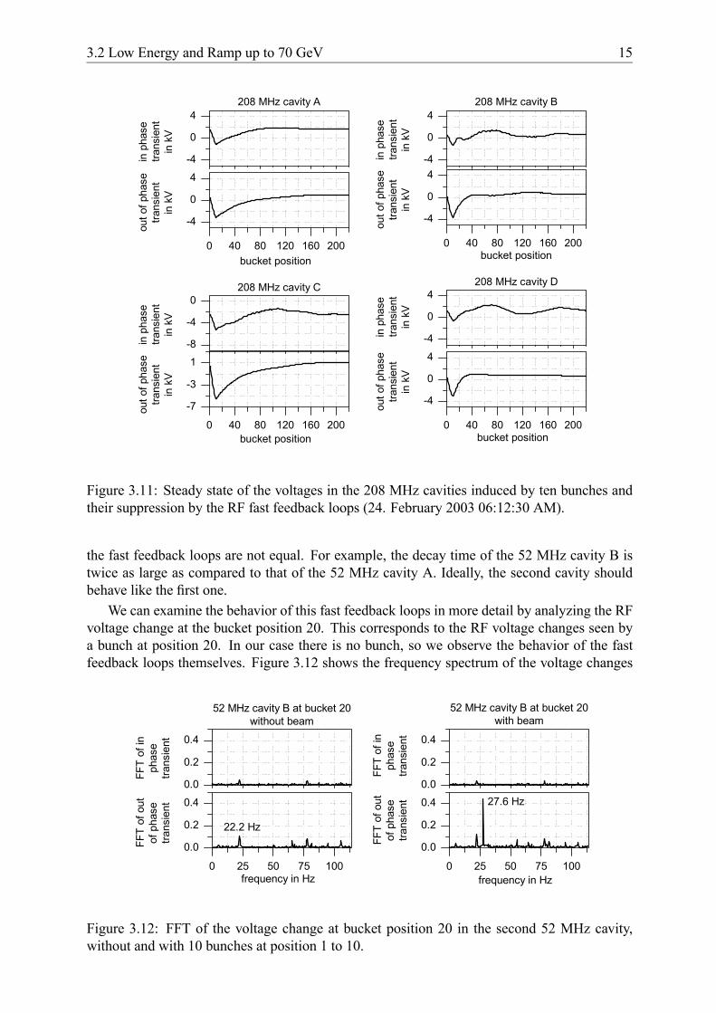
3.2 Low Energy and Ramp up to 70 GeV 15
-4
0
4
0 40 80 120 160 200
-4
0
4
-4
0
4
0 40 80 120 160 200
-4
0
4
-8
-4
0
0 40 80 120 160 200
-7
-3
1
-4
0
4
0 40 80 120 160 200
-4
0
4
208 MHz cavity A
in p
hase
trans
ient
in k
V
bucket position
ou
t of p
hase
trans
ient
in k
V
208 MHz cavity B
in p
hase
trans
ient
in k
V
bucket position
out o
f pha
setra
nsie
ntin
kV
208 MHz cavity C
in p
hase
trans
ient
in k
V
bucket position
out o
f pha
setra
nsie
ntin
kV
208 MHz cavity D
in p
hase
trans
ient
in k
V
bucket position
out o
f pha
setra
nsie
ntin
kV
Figure 3.11: Steady state of the voltages in the 208 MHz cavities induced by ten bunches andtheir suppression by the RF fast feedback loops (24. February 2003 06:12:30 AM).
the fast feedback loops are not equal. For example, the decay time of the 52 MHz cavity B istwice as large as compared to that of the 52 MHz cavity A. Ideally, the second cavity shouldbehave like the first one.We can examine the behavior of this fast feedback loops in more detail by analyzing the RF
voltage change at the bucket position 20. This corresponds to the RF voltage changes seen bya bunch at position 20. In our case there is no bunch, so we observe the behavior of the fastfeedback loops themselves. Figure 3.12 shows the frequency spectrum of the voltage changes
0.0
0.2
0.4
0 25 50 75 100
0.0
0.2
0.40.0
0.2
0.4
0 25 50 75 100
0.0
0.2
0.4
52 MHz cavity B at bucket 20without beam
FFT
of in
phas
etra
nsie
nt
22.2 Hz
frequency in Hz
FFT
of o
utof
pha
setra
nsie
nt
52 MHz cavity B at bucket 20with beam
FFT
of in
phas
etra
nsie
nt
27.6 Hz
frequency in Hz
FFT
of o
utof
pha
setra
nsie
nt
Figure 3.12: FFT of the voltage change at bucket position 20 in the second 52 MHz cavity,without and with 10 bunches at position 1 to 10.

16 Observed Emittance Dilution Effects
in the 52 MHz cavity B first without and with beam. With beam a remarkable line at 27.6 Hzappears. All other cavities do not show this line or only with much lower strength, see figure3.13.
0.0
0.2
0.4
0 25 50 75 100
0.0
0.2
0.40.0
0.2
0.4
0 25 50 75 100
0.0
0.2
0.4
0.0
0.2
0.4
0 25 50 75 100
0.0
0.2
0.40.0
0.2
0.4
0 25 50 75 100
0.0
0.2
0.4
0.0
0.2
0.4
0 25 50 75 100
0.0
0.2
0.4
0.0
0.2
0.4
0 25 50 75 100
0.0
0.2
0.4
52 MHz cavity A at bucket 20
FFT
of in
phas
etra
nsie
nt
frequency in Hz
FFT
of o
utof
pha
setra
nsie
nt52 MHz cavity B at bucket 20
FFT
of in
phas
etra
nsie
nt
27.6 Hz
frequency in Hz
FFT
of o
utof
pha
setra
nsie
nt
208 MHz cavity A at bucket 20
FFT
of in
phas
etra
nsie
nt
frequency in Hz
FFT
of o
utof
pha
setra
nsie
nt
208 MHz cavity B at bucket 20
FFT
of in
phas
etra
nsie
nt
frequency in Hz
FF
T of
out
of p
hase
trans
ient
208 MHz cavity C at bucket 20
FFT
of in
phas
etra
nsie
nt
27.6 Hz55.2 Hz
frequency in Hz
FFT
of o
uof
pha
setra
nsie
nt
208 MHz cavity D at bucket 20
FFT
of in
ph
ase
trans
ient
frequency in Hz
FFT
out
of p
hase
trans
ient
Figure 3.13: FFT of the voltage changes at bucket position 20 in all RF cavities, with 10 bunchesat position 1 to 10.

3.3 Coupled Bunch Oscillations above 70 GeV 17
3.3 Coupled Bunch Oscillations above 70 GeVThe strongest longitudinal emittance blow up occurs during the acceleration process above70GeV and at high energy, due to coupled bunch oscillations, as reported in [10]. Figure 3.14shows the development of the longitudinal emittance during acceleration derived from an analy-sis of recent FLD data. The origin of the time scale corresponds to the start of the acceleration.
0
100
200
300
400
-10 0 10 20 30 40 50 60
0
200
400
600
800
blow up causedby coupled
bunchoscillation
(modes l = 1, l = 164)
11.02.2003 05:08 PM 57 mA 16.01.2003 01:33 AM 32 mA 24.02.2003 06:09 PM 25 mA 27.01.2003 09:05 PM 17 mA
aver
age
of b
unch
em
ittan
ce(F
WH
M) i
n m
eVs
ener
gy in
GeV
time in min
Figure 3.14: Development of the longitudinal proton emittance in HERA during accelerationof 180 bunches from 40 GeV to 920 GeV. The sudden steps are caused by coupled bunchoscillations.
At this time, the initial longitudinal FWHM emittance is about 45 meVs to 70 meVs. Due tothe injection of the second and third bunch train, the average emittance changes are caused bybeam loading, see section 3.1, and the new injected bunches are also considered in the emittancemean value after an injection. This explains the appearance of the partly observable emittancereduction at injection in figure 3.14.At the ramps shown, the emittance grows smoothly up to energies around 300 GeV. Above
300 GeV the emittance is blown up in several vast steps. The analysis of the FLD data showsthat these steps are caused by coupled bunch oscillations. Figure 3.15 shows for example thecoupled bunch oscillation responsible for the marked step in figure 3.14. Even when 920GeVis reached with a relatively small emittance of 220 meVs, the beam behaves unstably, as theramp from 16th January indicates.As an example, consider the coupled bunch oscillation shown in figure 3.15. An interested

18 Observed Emittance Dilution Effects
0 20 40 60 80 100 120 140 160 180 200
time
ins
bucket number219
0
-0.5
+0.5
colo
r sca
le in
°
0.000
0.200
0.400
0.600
0.800
1.000
1.200
1.400
1.600
1.800
2.000
2.224
Figure 3.15: This coupled bunch oscillation took place on 16. January 2003 01:50:48 AM at368GeV, that was 17 minutes after the ramp started. It increased the longitudinal emittancefrom 100 meVs to 127meVs in a sudden step.
0 25 50 75 1001
10
100
0 25 50 75 100 125 150 175 200
0.00.20.40.60.81.0
46.7 Hz
frequency in Hz
num
ber o
fbu
nche
s
1641
mode number
porti
on o
fm
ode
Figure 3.16: Steady state modal analysis of the coupled bunch oscillation of 16. January 200301:50:48 AM. The mean frequency is 46.5 Hz and the synchrotron frequency spread 0.6 Hz.
reader, having access to the HERA control system and the FLD, may convince himself thatthe oscillation shown is typical and one can find much more impressive examples! Figure 3.16shows the result of the steady state modal analysis of the coupled bunch oscillation. For theunderlying principles of this analysis, see [3]. Nearly all bunches are oscillating with the samefrequency of 46.7 Hz, as the frequency distribution histogram shows. They are formed in the

3.3 Coupled Bunch Oscillations above 70 GeV 19
modes l = 1 and l = 164. The oscillation leads to a bunch lengthening within 22 seconds,shown in figure 3.17. After the bunches got longer, they are stabilized by the larger incoherent
1.2
1.4
0 50 100 150 200
1.2
1.4
bunc
h le
ngth
in n
sat
368
GeV
bucket position
bunc
h le
ngth
in n
sat
389
GeV
Figure 3.17: Lengthening of the bunches due to the coupled oscillation of 16. January 200301:50:48 AM. The upper graph shows the bunch lengths at 01:50:48 AM and the lower 22seconds later, at 01:51:33 AM. Aside, the shown bunch lengths are recalibrated with CMFL-data.
0 25 50 75 1001
10
100
0 25 50 75 100 125 150 175 200
0.00.20.40.60.81.0
frequency in Hz
num
ber o
fbu
nche
s
mode number
porti
on o
fm
ode
Figure 3.18: Steady state modal analysis of the coupled bunch oscillation of 16. January 200301:51:11 AM. The mean frequency is 41.9 Hz and the synchrotron frequency spread is 1.9 Hz.
synchrotron frequency spread and also by oscillating with different frequencies, see figure 3.18.From the mean frequency change, between the coupled oscillation and the free oscillation, onemay estimate the coupling impedance. The frequency spread of 1.9 Hz which is obviouslyable to suppress the coupling, may also be taken to estimate the impedance. Such estimatesare already discussed in [3]. But, for the situation presented we have also to consider thesynchrotron frequency change due to the changing RF voltages and particle energy during the

20 Observed Emittance Dilution Effects
acceleration. This change may seriously influence the results, especially when we estimate thecoupling impedance from the change of the mean frequency. A more proper way is to examinecoupled bunch oscillations taking place after high energy is reached, where the synchrotronfrequency of non coupled bunches is no longer changing. Nevertheless, such considerationsgive rise to the assumption that the longitudinal impedance budget got worse as compared to thesituation in HERA I. The problems discussed in section 3.2 in the RF systemmay be responsiblefor this behavior.
3.4 RF Noise EffectsPreservation of the longitudinal emittance during acceleration will result in shorter protonbunches at the begin of a luminosity run. To keep the bunches short we have also to sup-press longitudinal emittance diluting effects taking place during long beam storage times. Sucheffects are expected to be also responsible for protons kicked out of the bucket potential formingcoasting beam.The most obvious candidate, RF noise, was examined by S. Ivanov and O. Lebedev2 [8, 9],
as already mentioned. They measured the RF noise spectra by modifying the RF signal pathsof the cavity voltage measurements of the FLD, by substituting RF filters and amplifiers. Thenoise spectra taken from the 208MHz cavities show somewhat lower noise levels than expected.In contrast, the levels in the 52 MHz cavities are noticeable higher. Discrete frequency linesoverlay the continuous noise spectra. In the spectrum of the second 52 MHz cavity a strongline at about 30 Hz is present, which is not visible with the same strength in the other cavities.In their measurements, this line is visible both with and without beam. As the synchrotronfrequency at high energy is close to 35 Hz, this line is expected to have a significant influenceon the long term development of the longitudinal emittance and the production of coastingbeam.
0.00
0.05
0.10
0 200 400 600 800
0.00
0.05
0.10
0.00
0.05
0.10
0 200 400 600 800
0.00
0.05
0.10
52 MHz cavity A at bucket 30
FFT
of in
phas
etra
nsie
nt
frequency in Hz
FFT
of o
utof
pha
setra
nsie
nt
52 MHz cavity B at bucket 30
FFT
of in
phas
etra
nsie
nt
28.5
Hz
frequency in Hz
FFT
of o
utof
pha
setra
nsie
nt
Figure 3.19: FFT of the voltage changes in the 52 MHz cavities. The data record was takenon 1. March 2003 07:31:28 AM with 21 mA beam in 180 bunches at 920 GeV. In the second52MHz cavity a line at 28.5 Hz is visible.
The way in which the FLD takes the cavity voltage data is in no way adjusted for RF noisemeasurements as compared to the method from S. Ivanov and O. Lebedev. Nevertheless, byexamining the records taken, one discovers at high energy also a frequency line at 28.5Hz in
2both from Institute for High Energy Physics (IHEP) Protvino, Moscow Region, 142281, Russia

3.4 RF Noise Effects 21
the spectrum of the second 52 MHz cavity, see figure 3.19, which is not observable in the othercavities, figures 3.19 and 3.20.
0.00
0.05
0.10
0 200 400 600 800
0.00
0.05
0.10
0.00
0.05
0.10
0 200 400 600 800
0.00
0.05
0.10
0.00
0.05
0.10
0 200 400 600 800
0.00
0.05
0.10
0.00
0.05
0.10
0 200 400 600 800
0.00
0.05
0.10
208 MHz cavity A at bucket 30FF
T of
inph
ase
trans
ient
frequency in Hz
FFT
of o
utof
pha
setra
nsie
nt208 MHz cavity B at bucket 30
FFT
of in
phas
etra
nsie
nt
frequency in Hz
FFT
of o
utof
pha
setra
nsie
nt
208 MHz cavity C at bucket 30
FFT
of in
phas
etra
nsie
nt
frequency in Hz
FFT
of o
uof
pha
setra
nsie
nt
208 MHz cavity D at bucket 30
FFT
of in
ph
ase
trans
ient
frequency in Hz
FF
T ou
tof
pha
setra
nsie
nt
Figure 3.20: FFT of the voltage changes in the 52 MHz cavities. The data record was takenon 1. March 2003 07:31:28 AM. There are no frequency lines visible near the synchrotronfrequency of 20 Hz to 40 Hz.
In addition, the strong lines at 150Hz, 250Hz may be caused by the mains frequency. Amore detailed examination has to verify to what extent they are artificial, that means, caused inthe diagnostics system itself. The absence of the lines in most of the 208 MHz systems may bea hint, that these lines are real RF modulations of the cavity voltages.

22 Observed Emittance Dilution Effects
4 Tested Measures for EmittancePreservation
Beam oscillations, leading to an emittance dilution, may be suppressed by active or passivemethods. Active methods are control loops detecting the beam oscillations. Dependent on thedetected values, they steer devices acting back on the beam. Typical examples are narrow bandfeedbacks, like the so called ‘Phase Loop II’ at HERA, broad band feedbacks, this meanscoupled bunch feedbacks or a mixtures of both, like the ‘Phase Loop I’. In contrast, passivemethods increase the intrinsic damping of the beam without considering whether the beam isoscillating or not. For example, Landau damping cavities increase the incoherent synchrotronfrequency spread and with that the beam stability. One may also increase the coherent frequencyspread. This can be done by h+ 1 harmonic cavities or even an amplitude modulation (AM) ofthe RF voltage. With both methods, each bunch gets its one bucket potential strength and withthat its own synchrotron frequency.In this chapter, some of these measures, applied to the HERA proton ring and the experience
we made, will be discussed.
4.1 The Use of the Phase LoopsAt the HERA proton ring, two phase loops with different bandwidth and different control theo-retical principles are installed.The ‘Phase Loop I’ realizes a differential controller and works as follows: The circulating
beam is divided in 22 parts without particular consideration of the actual fill pattern. For eachof these 22 parts, the beam phase is measured and fed back as a phase change of the 52 MHzsteering signal with a programmable but fixed time delay. This time delay has to be near 1/4of a synchrotron oscillation cycle. Ideally, this delay time is changed from outside duringacceleration following the change of the synchrotron frequency. Until now, this has not beenthe case at HERA. The loop should damp the coupled bunch modes l ≤ 22.Using the default settings of the Phase Loop I, we found with the FLD that this loop is
only able to damp beam phase oscillations down to amplitudes of about 2◦ (52 MHz). Beamoscillations with amplitudes smaller than 2◦ are not influenced. This may be an indication thatthe sensor part of this loop is not very sensitive. Unfortunately, technical problems with theremote control of the loop parameters prevented a more careful examination. In the actualsituation, the loop is unsuitable for our purpose, because beam oscillations with amplitudessmaller than 2◦ already lead to a large emittance dilution.The ‘Phase Loop II’ realizes an integral controller in the following way: The beam phase is
measured with a sensitive narrow band phase detector. Beam phase deviations are transferredto changes of the RF frequency. These frequency changes result in the course of time in phasechanges, acting back on the beam. One can show that such a loop is inherently stable. Hence,very large feed back gains are possible. For more details within this respect, see [3]. But, theloop is only able to damp the coupled bunch mode l = 0.In the last HERA run period, the Phase Loop II became the focus of our attention, since the
longitudinal proton emittance suffered from beam phase oscillations at low energy in the mode
23

24 Tested Measures for Emittance Preservation
l = 0, as discussed in section 3.2. The loop is an ideal device to suppress these oscillations,as long we localize and eliminate the source driving them. For this purpose, the Phase LoopII should work without restrictions at low energy and during acceleration. Unfortunately, ourfirst attempts to use the loop during acceleration in September 2002, resulted in a confusion inthe timing between revolution triggers, bunch clock signals and the beam. In some cases, thiswas accompanied by high losses of beam intensity. Figure 4.1 shows such an effect, where the
0 20 40 60 80 100 120 140 160 180 2000.000
0.200
0.400
0.600
0.800
1.000
1.200
1.400
1.600
1.800
2.000
time
in s
bucket number219
2.224
0
-0.5
+0.5
colo
r sca
le in
°
Figure 4.1: A working Phase Loop II during acceleration caused until autumn 2002 suddenshifts between timing signals and the beam. Here, the jump of the FLD revolution triggerresulted in a FLD record showing a ‘jumped beam’. The record was taken on 9. September2002 at 60GeV with a beam current of about 5 mA.
revolution trigger, generated from the FLD timing, suffers a shift of about 150 bucket positions,resulting in a FLD record showing a jumped beam.Looking at such pictures, it must be clear, that the beam itself is not able to jump around the
storage ring. Therefore, they indicate a jumped timing. Not only the FLD timing jumped. Therevolution triggers of the HERA integrated timing (HIT) system jumped too.Since the loop consists of the phase detection of the beam, the whole HERA frequency gen-
eration, some RF phase locked loops and the controls for cavities, we had to take into accountall the technical details of these devices for localizing the bug. For an overview on the phaseloop and the timing systems, see figure 4.2.I will not bother the reader with all the discussions and measurements we performed. At
the end, Wilhelm Kriens, Uwe Hurdelbrink and Kai Brede from the group MSK found that thedata input at the frequency synthesizer had problems with lowering BCD values. This causedjumps in the HERA RF. These jumps were fast compared to a normal synchrotron oscillationcycle, so that the bunches were recaptured in RF buckets after the jumps and in most casesstill stored. Since the HIT and the FLD timing uses the RF as source to generate their signals,they also jumped. During acceleration without Phase Loop II, the frequency values increasedmonotonously and no problems arose. As the phase loop also reduces the frequency for shorttimes, to damp beam oscillations, the bug occurred.

4.1 The Use of the Phase Loops 25
52 MHzphaselockedloop
multi-plexer(digitaladding)
deter-mination
offrequency
52 MHzcavities
controlsfor twocavities
bunchedbeam
beam monitor
phasedet.LO RF
band pass
208 MHzcavities
controlsfor fourcavities
52 MHz 52 MHz
208 MHz
high passwith 0.3 Hz
ADCcontrollable
amplifier
BKR: “phaseloop II off/on“
choice ofloop gain
��
����f
FLDtiming
FECwith
ADCsBKR anddCache
HERAintegrated
timing(HIT)
52 MHzphaselockedloop
turn
trig
ger f
orch
eck
sync
hron
izat
ion
BCDnumbers
synthe-sizer
180 MHz
28 MHz20
8 M
Hz
gene
ratio
n
Figure 4.2: The Phase Loop II consists of a narrow band phase detection, whose output istransferred into a change of the frequency values at the RF synthesizer input. The generated208MHz RF frequency supplies the cavities controls with RF input signals, partly over a RFphase locked loop. Finally, the loop is closed over the beam. The timing systems use the 208MHz RF frequency to generate their clock and trigger signals.
Since the bug was fixed in autumn 2002, the loop works to our full satisfaction at low energy,during ramping and at high energy. Figure 4.3 contains an example for a beam oscillation atlow energy and its suppression after switching the loop on.
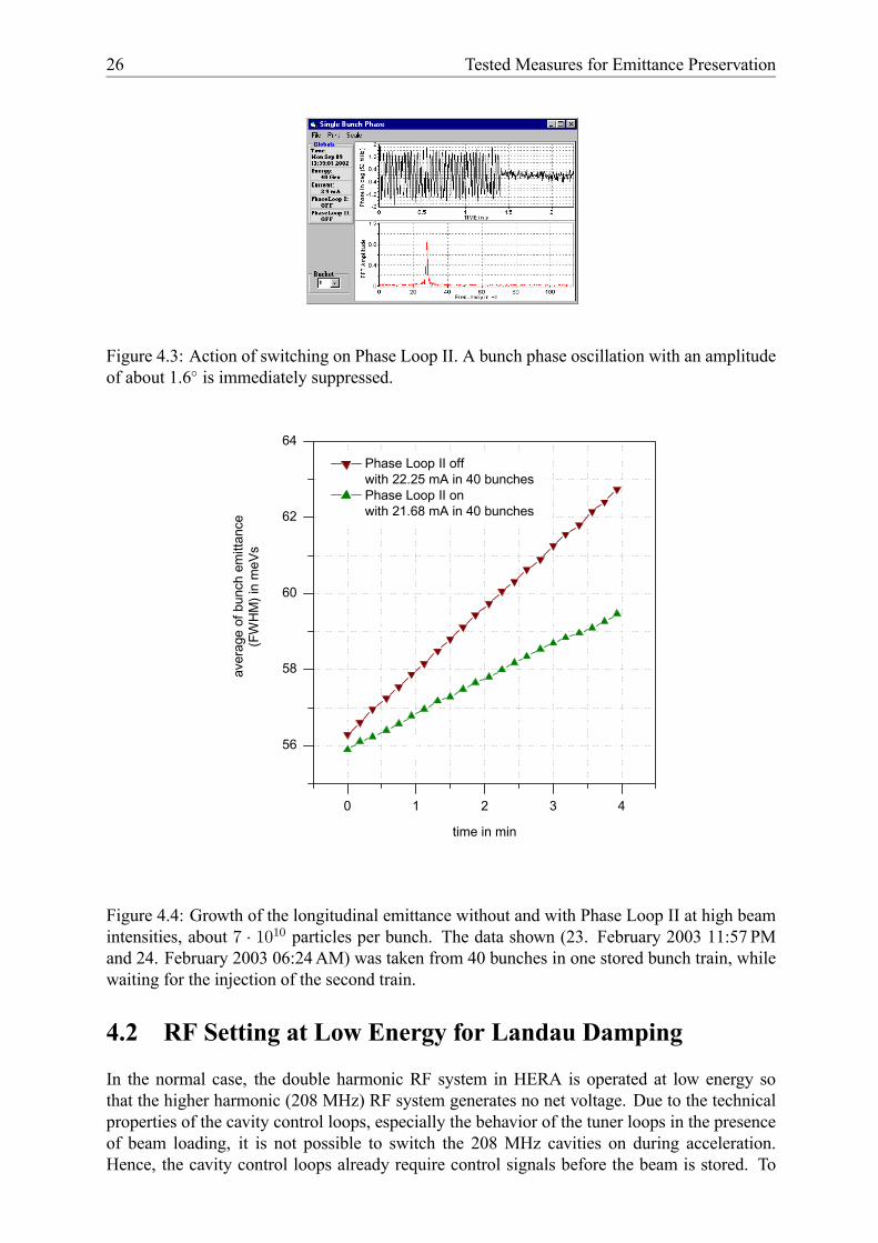
The loop does not only damp beam oscillations of coupled bunch mode l = 0, it has alsoa positive effect on the longitudinal emittance, as figure 4.4 shows for low energy and highbeam intensities. Without phase loop, the emittance increase in the case shown with about1.7meVs/min, the loop reduces this value to about 0.9meVs/min. This is a reduction of thegrowth rate of almost 1/2. At lower beam intensities the improvement achieved by the use ofthe loop was lower.
26 Tested Measures for Emittance Preservation
Figure 4.3: Action of switching on Phase Loop II. A bunch phase oscillation with an amplitudeof about 1.6◦ is immediately suppressed.
0 1 2 3 4
56
58
60
62
64
Phase Loop II off with 22.25 mA in 40 bunches Phase Loop II on with 21.68 mA in 40 bunches
aver
age
of b
unch
em
ittan
ce(F
WH
M) i
n m
eVs
time in min
Figure 4.4: Growth of the longitudinal emittance without and with Phase Loop II at high beamintensities, about 7 · 1010 particles per bunch. The data shown (23. February 2003 11:57 PMand 24. February 2003 06:24AM) was taken from 40 bunches in one stored bunch train, whilewaiting for the injection of the second train.
4.2 RF Setting at Low Energy for Landau Damping
In the normal case, the double harmonic RF system in HERA is operated at low energy sothat the higher harmonic (208 MHz) RF system generates no net voltage. Due to the technicalproperties of the cavity control loops, especially the behavior of the tuner loops in the presenceof beam loading, it is not possible to switch the 208 MHz cavities on during acceleration.Hence, the cavity control loops already require control signals before the beam is stored. To

4.2 RF Setting at Low Energy for Landau Damping 27
achieve zero voltage at injection, three 208 MHz cavities operate in phase, whose sum voltageis compensated by the fourth cavity, operating in counter phase.Normally, at low energy, the bucket potential is only provided by the 52 MHz system. By
changing the voltage of 208 MHz cavities we can use them as Landau damping cavities. Hence,we may increase the incoherent frequency spread sf = sω
2π. Typically, in a 4th harmonic Landau
damping system one uses a voltage for the higher harmonic RF system of about one fourth ofthe lower harmonic RF system in the bunch shortening mode, that mean, both voltages have thesame sign [11, 12].When h12 = h2
h1is the ratio of the harmonic numbers and r12 = V2
V1is the ratio of the RF
voltages, the frequency spread can be estimated for r12 < 1 / h12 and Gaussian bunches with
sω = − 116
1 + r12 h312√
1 + r12 h12ωs0 ∆φ2σ. (4.1)
In this expression, ωs0 is the synchrotron frequency for small oscillation amplitudes and V2 = 0.The half bunch length expressed in RF radians∆φσ can be obtained from
∆φσ =lFWHM
2β c√ln 4
2π h1 ωrev (4.2)
with the FWHMbunch length lFWHM, the RF frequency ωRF1 = h1 ωrev and β = vc. For Gaussian
bunches the relation between frequency spread and decoherence times is
τ d ≈ 0.655|sω | . (4.3)
A derivation of these formulae together with a discussion of their area of applicability is givenin [3].For a bunch length of lFWHM = 2.4 ns, we get a frequency spread of |sf | = 0.21Hz and a
decoherence time of 500ms when the 208 MHz voltage is zero and the synchrotron frequencyis fs0 ≈ 30Hz. By increasing the 208 MHz voltage to one fourth of the 52 MHz voltage weincrease the spread to |sf | = 2.5Hz and reduce the decoherence time to 40ms, leading to anadditional damping of beam phase oscillations.At HERA, a higher 208 MHz sum voltage can be obtained simply by a reduction of the volt-
age of the fourth cavity operating in counter phase. Figures 4.5 and 4.6 show the reduction ofthe bunch lengthening caused by injections when one lowers the voltage of the fourth 208MHzcavity by about 40 kV. The Phase Loop II was used in both cases to damp the coupled bunchmode l = 0. Without additional Landau damping, we observed in the case shown a bunchlengthening due to injections of about 40%. With additional Landau damping, introduced bythe 208 MHz RF system, we reduced this value to about 5%.Unfortunately, none of the data records from the injections without additional Lanuau damp-
ing, discussed with figure 4.5, show an injection process itself. Figure 3.3 shows also theeffect of an injection without additional 208MHz voltage, but with a higher beam current(69 mA). One observes a weakly damped beam oscillation with relatively long decoherencetime> 250ms. From the injection with additional Landau damping we have a data recordshowing directly an injection process. In figure 4.7 the phase, length and intensity of a alreadystored bunch is shown at the time of the injection of the third train. From the exponential decayof the bunch phase oscillation we obtain a decoherence time of about 40ms, which agrees withour calculations.The bunch shown suffered no loss of intensity. This was not the case for all bunches. The
data record shows intensity losses mainly at the newly injected bunches and only small losses at

28 Tested Measures for Emittance Preservation
2.4
2.8
3.2
3.6
2.4
2.8
3.2
3.6
0 20 40 60 80 100 120 140 160 180 200 220
2.4
2.8
3.2
3.6
bu
nch
leng
thin
ns
first
trai
n
bu
nch
leng
thin
ns
two
train
s
bucket number
bunc
h le
ngth
in n
sth
ree
train
s
Figure 4.5: Bunch lengthening during injection of three bunch trains with a final beam currentof 53 mA (21. February 2003 02:47 PM). The 208 MHz sum voltage was near zero and thePhase Loop II in operation.
2.4
2.8
3.2
3.6
2.4
2.8
3.2
3.6
0 20 40 60 80 100 120 140 160 180 200 220
2.4
2.8
3.2
3.6
bunc
h le
ngth
in n
sfir
st tr
ain
bunc
h le
ngth
in n
stw
o tra
ins
bucket number
bunc
h le
ngth
in n
sth
ree
train
s
Figure 4.6: Bunch lengthening during injection of three bunch trains with a final beam currentof 50 mA (22. February 2003 02:01 PM). The 208 MHz sum voltage was about 40 kV, this isaround 1/4 of the 52 MHz voltage of 140 kV. In this case, the Phase Loop II was in operation,too.

4.3 RF Amplitude Modulation 29
-2-1012
2.25
2.30
2.35
0.0 0.5 1.0 1.5 2.0
5.40
5.45
bu
nch
phas
e(n
o. 9
5)in
deg
(52
MH
z)
bu
nch
leng
thin
ns
time in sec
bunc
h in
tens
ityin
1010
par
ticle
s
Figure 4.7: Oscillation of the already stored bunch at position 95, increase of its length and theloss of intensity due to the injection of the third bunch train. To damp the beam oscillations,the 208 MHz sum voltage was about 1/4 of the 52 MHz voltage to introduce additional Landaudamping.
the first ten bunches. But these effects are small as compared to the situation without additional208MHz voltage.In the HERA run period before the luminosity upgrade, that was in 2000, we measured
decoherence times after applying particular RF kicks [3]. At that time, we measure decoherencetimes more comparable to the value obtained now with additional 208MHz voltage. In 2000,the 208MHz sum voltage was also programmed to be zero. To resolve these inconsistencies,we must re-examine the cavity voltage calibration.
4.3 RF Amplitude ModulationAn oscillating bunch leaves oscillating beam loading voltages and wake fields behind, actingon subsequent bunches. Bunches suffering a driving force oscillating with their synchrotronfrequency respond with the largest oscillation amplitudes. Hence, bunch oscillations result in achain reaction when all bunches have similar synchrotron frequencies, resulting in an coupledbunch oscillation, respectively instability. By giving each bunch its individual synchrotron fre-quency, we can interrupt this chain reaction and suppress coupled bunch instabilities. Variationsof the synchrotron frequencies over a bunch train require variations of the RF sum voltage seenby the individual bunches.
4.3.1 Using a h+ 1 cavityOne method to obtain a variation of the RF sum voltage is to operate some of the cavities in astorage ring with a slightly different harmonic number. For example, we may operate a cavity

30 Tested Measures for Emittance Preservation
with the harmonic number h+ 1. Then the sum voltage will vary from Vh − Vh+1 to Vh + Vh+1over one revolution, but every bunch still sees a constant voltage. This method was alreadydiscussed with h− 7 (h = 84) cavities in 1988 for the Fermilab Booster [13].Following the derivation in appendix A.1, we may obtain a bunch to bunch synchrotron
frequency spread Sf with a h+ 1 cavity at HERA of
Sffs0≈ 5 Vh+1
Vh, (4.4)
where fs0 is the small amplitude synchrotron frequency, Vh the ‘normal’ RF voltage and Vh+1the voltage of a cavity running at a h+ 1 harmonic RF frequency.According to Sacherer [14], a rule-of- thumb for de-coupling coupled bunch oscillations is
that the spread in individual bunch frequencies should exceed the frequency shift |∆fl| due tothe coupling:
(coherent) spread > shift (4.5)Sf > |∆fl| for de-coupling. (4.6)
In 3.3 we discussed the measurement of a frequency shift due to the coupling of about 2Hz.That means, we have to introduce a spread of Sf > 2Hz. To guarantee proper working RFcontrols, the minimum voltages at the HERA RF cavities are 30 kV (Vh+1). With a sum voltageVh at high energy of 540 kV this would result in a spread of Sf ≈ 8Hz> 2Hz, which shouldbe sufficient for suppressing the observed coupled bunch instabilities.However, a disadvantage of this method is a systematic variation of the bunch to bunch
spacing, lowering the luminosity. For example, a bunch centroid shift of 5◦ (52MHz), reducesthe luminosity at this collision by about 5% [15], because of the small β-function. For the ratiogiven above of Vh+1
Vh= 30 kV
520 kV we estimate with (A.10) maximum bunch phase deviations of±3.5◦. The resulting loss of luminosity may be tolerable. But, another problem may be thebucket matching at injection, and ensuring that all bunches have the same bucket potential forLandau damping, as discussed in section 4.2.
4.3.2 Direct RF amplitude modulationDuring the last HERA run period, we tested another possibility to increase the bunch to bunchsynchrotron frequency spread. We modulated the amplitude of the RF drive signals of cavitiesthemselves, without influencing the phasing. In contrast to a h+1 solution, this method requiresmore RF power. But it has some operational advantages. For example, one can easily switch iton and off during acceleration.Following the calculations of appendix A.2, the frequency spread introduced by the modu-
lation amplitude of Vmod is
Sffs0≈ 5 Vmod
V0for
VmodV0
< 0.6, (4.7)
where V0 is the RF voltage without amplitude modulation. To provide a spread of Sf > 2Hzwith fs0 ≈ 30Hz and V0 = 520 kV, we need a minimummodulation amplitude of about Vmod ≈7 kV. As we will see, such values are easily obtainable with the HERA proton RF systems.At injection energy we do not want to modulate that RF amplitude, which is required for
correct RF conditions during injections. As the coupled bunch instabilities occur at higherenergies, it is possible to delay the modulation until the transition from the 52MHz buckets tothe 208MHz buckets. This is the case at energies higher than 150 GeV, compare figure 4.8.

4.3 RF Amplitude Modulation 31
50
75
100
125
150
175
ener
gyin
GeV
time [ -10ns, 10ns]
RF
voltage[-150kV, 330kV
]
Figure 4.8: Bucket transition during acceleration of protons in HERA, starting from a 52 MHzbucket at injection to a 208 MHz bucket at higher energies. For comparison, typical FWHMbunch lengths at injection are 2.4 ns.
After reaching 150 GeV it is sufficient to modulate only the amplitude of 208 MHz cavities.The test setup used is shown in figure 4.9.To generate the envelope of the RF amplitude modulation (AM), we use a HP 8112A Pulse
Generator which is triggered by a revolution trigger supplied by the FLD timing. We adjustedthe generator to produce a triangular output signal in the range between±1V. By supplying thissignal to the I input of an IQ modulator, a 208 MHz RF signal is generated and added to thesteering signal of a cavity, as shown in figure 4.9. The cable length between the pulse generatorand the IQ modulator is experimentally adjusted so that at energies above 150GeV only the RFamplitude is influenced. As the signal combination is performed within the slow amplitude andphase regulation loop, possible errors in the mean RF values are automatically corrected. For amore detailed description of the RF system itself see [3].We are able to switch the modulation on and off via the GPIB connection of the pulse
generator to a UNIX workstation and to choose the modulation strength from a console in thecontrol room. The workstation and the software are very kindly serviced by Uwe Hurdelbrinkfrom the group MSK.The first graph in figure 4.10 shows the beam loading in the 208 MHz cavity A at 150
GeV. After switching the AM on, the RF voltage changes, so that a bunch at bucket 80 seesabout 80 kV less than one at bucket 205, as shown in the second graph in figure 4.10. With oursimple modulation technique, we also influence the phasing somewhat. A more sophisticated

32 Tested Measures for Emittance Preservation
amplifier
fastfeed-backloop
tunercontrolloop
amp. &phasecontrolloop
plungertuner beam
RF ref.signal
208 MHzcavity
GPIBremotecontrol
HP 8112APulse
Generator50 MHz
experimental setupfor amplitude
modulation
RF system
cond
ition
unit
amp.
rem
ote
cont
rol
of a
mpl
itude
�
diagnostic
rem
ote
cont
rol
of p
hase
revolution trigger fromFLD timing
50 �
FWDCOMP
input
I Q
resistivesplitter
tosecondcavity
IQ-modulator
Figure 4.9: Test setup for 208 MHz RF amplitude modulation to suppress coupled bunch oscil-lations.
-4
0
4
0 40 80 120 160 200
-4
0
4
-40
0
40
0 40 80 120 160 200
-40
0
40
208 MHz cavity A without AM
in p
hase
trans
ient
in k
V
bucket position
out o
f pha
setra
nsie
ntin
kV
208 MHz cavity A with AM
in p
hase
trans
ient
in k
V
bucket position
out o
f pha
setra
nsie
ntin
kV
Figure 4.10: Measured beam loading at 150 GeV before and after switching on the amplitudemodulation (26. February 2003 06:48 PM).
method may eliminate these phase changes. We will discuss that in the next chapter. But, forthe moment we will neglect these small phase changes.

4.3 RF Amplitude Modulation 33
4.3.3 Experiences made with the direct RF amplitude modulationBefore using the amplitude modulation (AM) during a standard proton acceleration, we per-formed several tests. First, we tested, whether the RF system itself tolerated such modulationswithout malfunction without beam, followed by tests with stored beam at 920 GeV. Havingencountered no problems, we extended our activities to normal proton accelerations duringstandard HERA operation. In January and February 2003, the AM was in operation during 16ramps. On seven occasions it was active during the whole proton storage at 920 GeV. Withthe exception of one instance, it never caused beam losses, in the most unfortunate cases thecoupled bunch instabilities were not suppressed and we observed bunch lengths comparable tothose after ramps without AM. The event with beam loss was caused by an operating error.During the first ramps with modulation, we used only one 208 MHz cavity to provide a AM
between 30 kV and 40 kV. As we still observed coupled bunch oscillations, we also applied themodulation to a second cavity, to double the amplitude. It turned out, that permanent use of thePhase Loop II together with the AM is necessary, to successfully suppress the instabilities.
-10 0 10 20 30 40 50 60
0
100
200
300
400
AM on (150 GeV)
blow up causedby coupled
bunchoscillation
(modes l = 1, l = 164)
920 GeVreached
'normal' ramp of 32 mA ramp of 32 mA with AM
aver
age
of b
unch
em
ittan
ce(F
WH
M) i
n m
eVs
time in min
Figure 4.11: Two ramps (both 16. January 2003) with similar beam current, one with and onewithout amplitude modulation.
Permanent use of the Phase Loop II result in some operational difficulties for the synchro-nization of the electron ring to the proton ring. As both the synchronization and the phase loopinfluence the frequency generation, one has to supervise the difference frequency between bothrings to be positive during the synchronization process. If the phase loop responds to a beamoscillation such, that this difference frequency would become negative, the synchronization willnot lock the correct bucket positions of both rings on each other. Then, the electron buncheswould not hit the proton bunches within the experiments H1 and ZEUS. If one detects the possi-bility of negative difference frequencies, one has to switch the phase loop off during the lockingprocess of the synchronization. Afterwards it has to be immediately switched on. For details onthe principles of the synchronization loop and the Phase Loop II, see [3].

34 Tested Measures for Emittance Preservation
To get an impression of the effect achieved by the AM, we will here compare pairs of protonramps with similar beam current. Figure 4.11 show as first example the development of the lon-gitudinal emittance during ramps performed on 16th January, each with a proton beam currentof 32 mA. Without AM, the beam suffered coupled bunch instabilities causing a stepwise blowup of the longitudinal emittance. The RF modulation applied to one 208 MHz cavity, with anamplitude of about 37 kV, generated a bunch to bunch synchrotron frequency spread, suppress-ing coupled bunch instabilities. Although there were some beam oscillations visible during theramp with AM, the emittance was more than a factor of two smaller as compared to the valuereached without modulation.
-10 0 10 20 30 40 50 60
0
100
200
300
400
AM on (150 GeV)
coupledbunch
oscillation
AM off(Phase Loop II off)
coupled bunchoscillation
920 GeVreached
'normal' ramp of 25 mA ramp of 27 mA with AM
aver
age
of b
unch
em
ittan
ce(F
WH
M) i
n m
eVs
time in min
Figure 4.12: Two ramps (24. and 26. February) with nearly similar beam current of about26mA. To perform a cross check of the action of the modulation and phase loop, we switchedboth off, 12 minutes after reaching problem-free 920GeV.
The efficacy of the AM can also be checked in the following way: We accelerate protonswith the amplitude modulation, to suppress the instabilities and get short bunches at high energy.We ensure that the beam is stable, by waiting with active AM and phase loop for some time afterreaching 920GeV. For example we wait 10 minutes. Then, we switch off both, the AM and thephase loop and observe, whether coupled bunch oscillations arise, causing an emittance blowup. Figure 4.12 shows the result of an test of this idea. In contrast to the ramp shown infigure 4.11, we applied the modulation onto two 208 MHz cavities, resulting in an modulationamplitude of 78 kV. During this ramp (AM on), no strong beam oscillation was visible. In thiscase, we got also a reduction of the longitudinal emittance of an factor of two due to the AM.The corresponding bunch lengths are about 0.97 ns. After switching the AM and the phase loopoff, a strong coupled bunch oscillation occurred resulting in a considerable emittance blow up.The bunch length increased to typical values of about 2 ns. For completeness, figure 4.13 showsthe beam oscillation which arose.

4.3 RF Amplitude Modulation 35
0 20 40 60 80 100 120 140 160 180 2000.000
0.025
0.050
0.075
0.100
0.125
0.150
0.175
0.200
0.225
0.250
time
in s
bucket number219
0.278
0
-3
+3
colo
r sca
le in
°
Figure 4.13: This coupled bunch oscillation occurred after switching the AM and the phaseloop off at 920 GeV and initial bunch lengths of 0.97 ns (26. February 2003 07:21:04 PM).
-10 0 10 20 30 40 50 60
0
100
200
AM on(150 GeV)
coupled bunchoscillations
during wholeramp above
300 GeV
920 GeVreached
ramp of 27 mA without AM and without Phase Loop II ramp of 29 mA with AM and with Phase Loop II
aver
age
of b
unch
em
ittan
ce(F
WH
M) i
n m
eVs
time in min
Figure 4.14: Again two ramps (08. and 10. February) with nearly similar beam current of about28 mA. After both ramps the protons was successfully brought into collision with electrons.

36 Tested Measures for Emittance Preservation
The final goal of the activities presented here, is to make luminosity with short bunches.Therefore, we had to show that this is possible in practice without problems. Figure 4.14 showsagain two ramps with comparable beam current. By permanently using the Phase Loop II andswitching the AM on at 150 GeV, we obtained a longitudinal emittance at 920 GeV which wasnearly a factor of two smaller, as compared to a ramp without phase loop and without AM.After both ramps the proton beams was successfully brought into collision with electron beams,resulting in nearly the same specific luminosity of about 2 1030
cm2 s mA2 , measured at H1. This isslightly over the design value of 1.8 1030
cm2 s mA2 .
0
1
2
0 60 120 180 240 300 360 420 480 540 600 660
spez
ific
lum
iat
H1
in10
30 c
m-2 s
-1 m
A-2
1.01.52.02.5
bunc
hle
nght
hin
ns
0
100
200
emitt
ance
in m
eVs
0
400
800
prot
onen
ergy
in G
eV
0102030
prot
oncu
rrent
in m
A
0102030
elec
tron
curre
ntin
mA
0 60 120 180 240 300 360 420 480 540 600 6600246
time in min
anod
e cu
rrent
of 2
08 M
Hz
cavi
ty 1
in A
Figure 4.15: Luminosity run on 10. February with Phase Loop II permanently in operation andAM in operation from 10 min to 630 min.
Figure 4.15 shows the longitudinal beam behavior during the luminosity run with AM andphase loop in operation. For orientation, the AM was switched on 10 min after the proton rampstart, which is the origin of time scale in figure 4.15. It was then in operation for 620 min. After
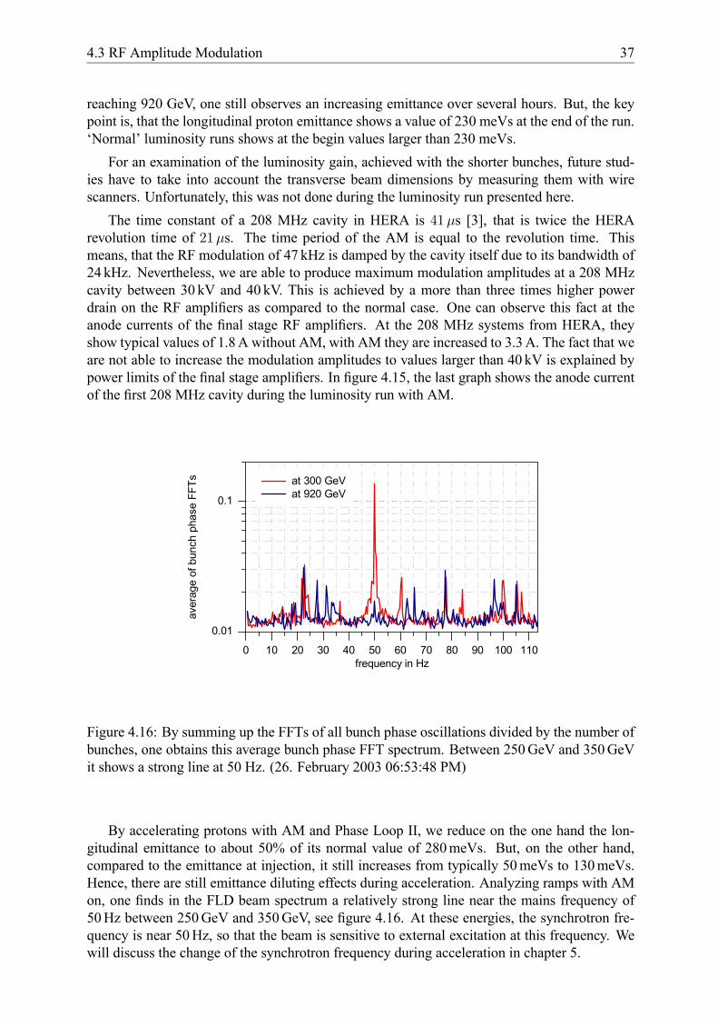
4.3 RF Amplitude Modulation 37
reaching 920 GeV, one still observes an increasing emittance over several hours. But, the keypoint is, that the longitudinal proton emittance shows a value of 230 meVs at the end of the run.‘Normal’ luminosity runs shows at the begin values larger than 230 meVs.For an examination of the luminosity gain, achieved with the shorter bunches, future stud-
ies have to take into account the transverse beam dimensions by measuring them with wirescanners. Unfortunately, this was not done during the luminosity run presented here.The time constant of a 208 MHz cavity in HERA is 41µs [3], that is twice the HERA
revolution time of 21µs. The time period of the AM is equal to the revolution time. Thismeans, that the RF modulation of 47 kHz is damped by the cavity itself due to its bandwidth of24 kHz. Nevertheless, we are able to produce maximum modulation amplitudes at a 208 MHzcavity between 30 kV and 40 kV. This is achieved by a more than three times higher powerdrain on the RF amplifiers as compared to the normal case. One can observe this fact at theanode currents of the final stage RF amplifiers. At the 208 MHz systems from HERA, theyshow typical values of 1.8A without AM, with AM they are increased to 3.3A. The fact that weare not able to increase the modulation amplitudes to values larger than 40 kV is explained bypower limits of the final stage amplifiers. In figure 4.15, the last graph shows the anode currentof the first 208 MHz cavity during the luminosity run with AM.
0 10 20 30 40 50 60 70 80 90 100 110
0.01
0.1
at 300 GeV at 920 GeV
frequency in Hz
aver
age
of b
unch
pha
se F
FTs
Figure 4.16: By summing up the FFTs of all bunch phase oscillations divided by the number ofbunches, one obtains this average bunch phase FFT spectrum. Between 250GeV and 350GeVit shows a strong line at 50 Hz. (26. February 2003 06:53:48 PM)
By accelerating protons with AM and Phase Loop II, we reduce on the one hand the lon-gitudinal emittance to about 50% of its normal value of 280meVs. But, on the other hand,compared to the emittance at injection, it still increases from typically 50meVs to 130meVs.Hence, there are still emittance diluting effects during acceleration. Analyzing ramps with AMon, one finds in the FLD beam spectrum a relatively strong line near the mains frequency of50Hz between 250GeV and 350GeV, see figure 4.16. At these energies, the synchrotron fre-quency is near 50Hz, so that the beam is sensitive to external excitation at this frequency. Wewill discuss the change of the synchrotron frequency during acceleration in chapter 5.

38 Tested Measures for Emittance Preservation
4.3.4 Actual limits of the direct RF amplitude modulationThe method worked without problem at all ramps of beam currents up to 32 mA in 180 bunches.During two ramps with beam current of about 48 mA in 180 bunches, we suppressed all coupledbunch oscillations up to 915GeV. But unfortunately, before reaching 920 GeV the beam becameunstable and the bunches long. A ramp of 52 mA in 120 bunches in three trains, as shown forexample in figure 4.6, with AM and Phase Loop II resulted in short bunches without instabilities.This observation should be explained by the fact, that gaps in the occupation pattern result in amore stable behavior [16].
4.4 RF Setting at High EnergyAfter reaching short bunches at high energy, the next task is to keep them as short as possibleduring luminosity operation. As already mentioned in section 3.4, the second 52 MHz cavityshows a line at about 28Hz in the RF frequency spectrum. As the synchrotron frequency isnear 30Hz at high energy, the question arose whether this ‘noise’ leads to emittance dilutionduring long storage times. To verify that, we kept the sum voltage of both 52 MHz cavities at
2 4 6 8 10 12 14 16 18 20 22
1.7
1.8
1.9
2.0
2.1
start oflumi runs
52 MHz cavity A = 70 kV and 52 MHz cavity B = 70 kV with 45 mA 52 MHz cavity A = 110 kV and 52 MHz cavity B = 30 kV with 48 mA
aver
age
FLD
bun
ch le
ngth
(FW
HM
) in
ns
time in h
Figure 4.17: Two nearly similar luminosity runs (15. February and 16. February 2003) withequal 52 MHz sum voltages at high energy. A reduced voltage in the 52 MHz cavity B resultedin a significant smaller bunch lengthening rate.
140 kV during two luminosity runs with equal conditions in beam current, initial bunch lengthetc. During one run, the 52 MHz voltage was provided by equal voltages in both cavities. Thiswas the normal case until then. During the other run, the voltage of the second 52MHz cavitywas reduced to 30 kV, and the first one increased to 110 kV. On the assumption that the 28 Hzline in the second 52 MHz cavity scales with the cavity voltage, we expected to see a differencein the bunch lengthening, taking pace during several hours at luminosity operation.

4.4 RF Setting at High Energy 39
Figure 4.17 shows the result of this examination. Before the start of luminosity operation,both runs shows nearly similar bunch lengthening rates. After bringing both beams into colli-sion, a significant difference in the bunch lengthening is visible. To first order, the run with the70 kV in both cavities, shows a bunch lengthening of 17 ps/h. In contrast, the run with reducedvoltage in the second 52 MHz cavity shows a bunch lengthening of 11 ps/h. This is a reductionby 35%. Of course, one measurement alone could be a lucky shot. But, after solving the prob-lem with the second 52 MHz cavity in the shut down, we should measure a bunch lengtheningequal or smaller than 11 ps/h at beam currents of 48 mA.The 52 MHz cavities in the HERA proton ring are supplied with ferrite tuners [3]. Cavities
with such tuners produce in principle more RF noise as compared to cavities with plunger tuners[17]. To keep this noise component as low as possible, we operated HERA at high energy with30 kV in each of the 52MHz cavities, until the end of the run period.

40 Tested Measures for Emittance Preservation

5 Continue Fighting the Blow Up
In this chapter, we will discuss further measures for preserving the longitudinal emittance in theHERA proton ring. In view of the actual schedule to operate HERA II until January 2007, wewill only consider measures, which appear feasible before this deadline. In case of an approvalof HERA III [18], implying HERA operation after January 2007, some additional measureswould become noteworthy.
5.1 Further Debugging HERA LongitudinallyDuring the shutdown, taking place fromMarch to July 2003, examinations of the 52MHz cavityB and the accompanying control loops are planned to identify the source of the 28 Hz line in thespectrum. At the moment we are speculating on several possibilities, for example, malfunctionsof the control loop power supplies or mechanical resonances.The Phase Loop I should damp emittance diluting oscillations with l ≤ 22 perfectly, during
injection and acceleration. As the loop damps only oscillation amplitudes larger than 2◦, wehave first to examine the sensitivity of its beam phase oscillation detector. This detector hasprobably to be replaced by a more sensitive one. Furthermore, the remote control access to theloop parameters has to be replaced by a reliable one. This is essential to adjust loop parametersin dependence on the changing synchrotron frequency during acceleration. In the next section,we will see that the synchrotron frequency changes from about 30Hz at injection to 65Hz at110GeV and back to 35Hz at high energy. A fixed adjustment of the loop parameters fordamping synchrotron oscillations with 30Hz would anti-damp oscillations with 60Hz.For a more exact adjustment of the cavity voltage ramp tables, an improvement of the cavity
field calibration is advisable. This could be achieved by measuring the synchrotron frequency independence on different cavity voltage settings and correlating the results. At a constant energy,RF kicks could excite synchrotron oscillations which are then measured by the FLD.All possible sources, responsible for exciting the beam with the mains frequency (50 Hz)
should be eliminated. This may result in some work.
5.2 Examinations of new RF Voltage Ramp-TablesIn this report, we discussed some examinations, to improve the RF settings. We have to continuethese activities.During injection, we found that additional 208MHz voltage introduces Landau damping,
keeping the bunches short. In principle, it would be wise, to use this possibility and to try somefine tuning.At about 300 GeV we observed the mains frequency on the FLD beam data. Figure 5.1
shows the synchrotron frequency during acceleration, calculated from the values given in theRF ramp tables. The synchrotron frequency crosses the mains frequency twice. The crossingat 82Hz was not visible at the recorded FLD until now. This might be an indication, that thiscrossing is fast enough and causes no problems. But the crossing at 327 GeV is already visibleat 250 GeV up to 350 GeV. Hence, we have to think of changing the RF ramp tables in thisenergy region, for achieving a faster crossing of the mains frequency. Another option would
41
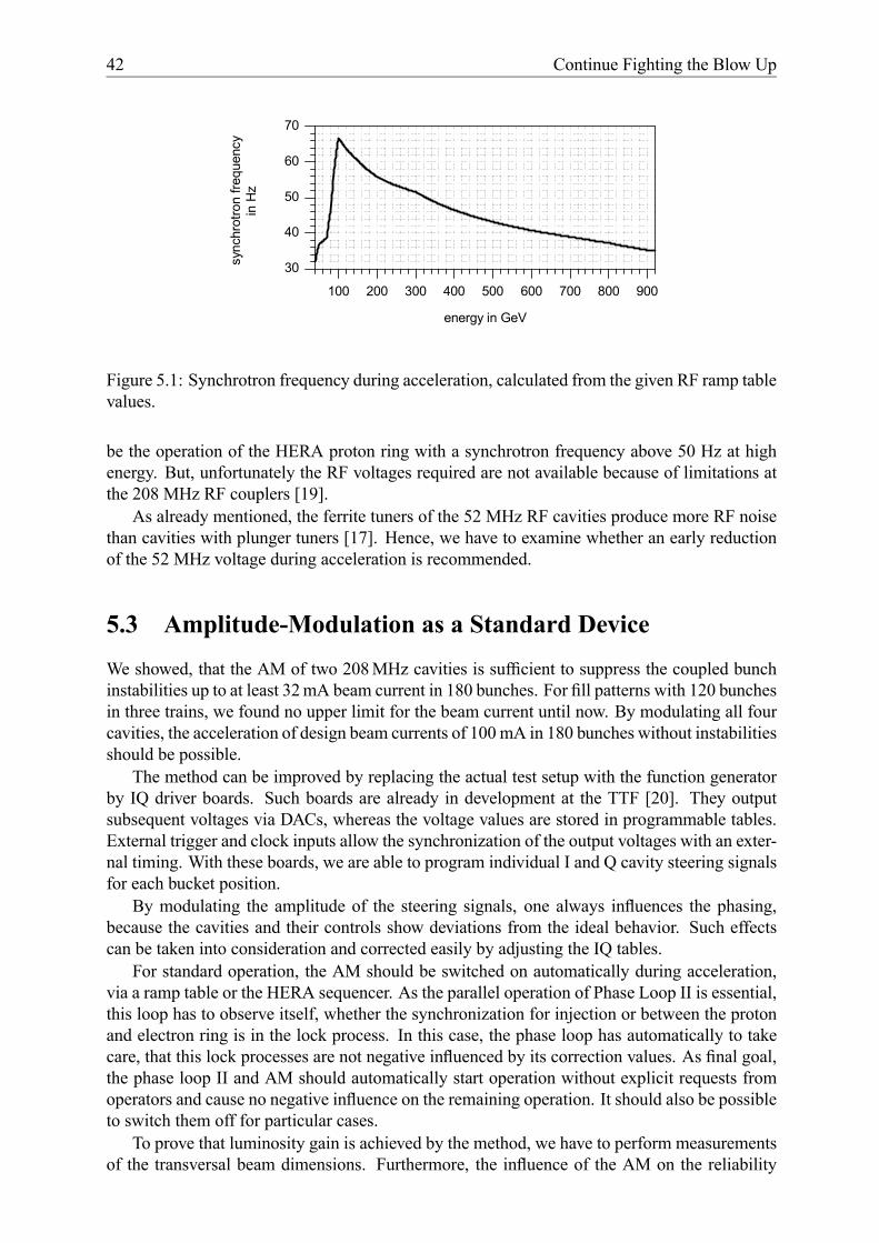
42 Continue Fighting the Blow Up
100 200 300 400 500 600 700 800 900
30
40
50
60
70
sync
hrot
ron
frequ
ency
in H
z
energy in GeV
Figure 5.1: Synchrotron frequency during acceleration, calculated from the given RF ramp tablevalues.
be the operation of the HERA proton ring with a synchrotron frequency above 50 Hz at highenergy. But, unfortunately the RF voltages required are not available because of limitations atthe 208 MHz RF couplers [19].As already mentioned, the ferrite tuners of the 52 MHz RF cavities produce more RF noise
than cavities with plunger tuners [17]. Hence, we have to examine whether an early reductionof the 52 MHz voltage during acceleration is recommended.
5.3 Amplitude-Modulation as a Standard Device
We showed, that the AM of two 208MHz cavities is sufficient to suppress the coupled bunchinstabilities up to at least 32mA beam current in 180 bunches. For fill patterns with 120 bunchesin three trains, we found no upper limit for the beam current until now. By modulating all fourcavities, the acceleration of design beam currents of 100 mA in 180 bunches without instabilitiesshould be possible.The method can be improved by replacing the actual test setup with the function generator
by IQ driver boards. Such boards are already in development at the TTF [20]. They outputsubsequent voltages via DACs, whereas the voltage values are stored in programmable tables.External trigger and clock inputs allow the synchronization of the output voltages with an exter-nal timing. With these boards, we are able to program individual I and Q cavity steering signalsfor each bucket position.By modulating the amplitude of the steering signals, one always influences the phasing,
because the cavities and their controls show deviations from the ideal behavior. Such effectscan be taken into consideration and corrected easily by adjusting the IQ tables.For standard operation, the AM should be switched on automatically during acceleration,
via a ramp table or the HERA sequencer. As the parallel operation of Phase Loop II is essential,this loop has to observe itself, whether the synchronization for injection or between the protonand electron ring is in the lock process. In this case, the phase loop has automatically to takecare, that this lock processes are not negative influenced by its correction values. As final goal,the phase loop II and AM should automatically start operation without explicit requests fromoperators and cause no negative influence on the remaining operation. It should also be possibleto switch them off for particular cases.To prove that luminosity gain is achieved by the method, we have to perform measurements
of the transversal beam dimensions. Furthermore, the influence of the AM on the reliability

5.4 Further Development of the FLD 43
of the final stage amplifiers and the cavity control systems has to be monitored, because of theincreased demand of RF power.
5.4 Further Development of the FLDSome essential work has still to be done at the FLD. This is first of all the automatic reading ofthe data stored at the dCache. At the moment, this data has to be copied by hand with severalUNIX commands before the analysis can take place.For future RF noise studies, the single bunch measurement has to be commissioned. With
this measurement, we will be able to record the bunch data of single bunches for time intervalsof up to 70 sec without gaps. Thus providing a solid basis for determinations of the beamspectrum with high resolution or sensitivity.The actual bunch length measurement fits in principle a Gaussian to the bunch shape at
two points, by measuring the 52MHz and the 208MHz bunch Fourier component. As long asthe bunch populations show similar distribution, this is sufficient. But unfortunately, coupledbunch oscillations tend to change the population at the bunch tails. This has an influence onthe resulting FLD bunch length. Figure 5.2 shows the same bunch during acceleration, oncebefore a coupled bunch oscillation and once afterwards. From the bunch shape, we determine
8 10 12
0.0
0.5
1.0 before instability after instability
sam
pled
sig
nal
(nor
mal
ized
to m
axim
um)
time in ns
Figure 5.2: Bunch shape of bunch no 5, before (170GeV) and after (820GeV) a coupled bunchinstability with equal FWHM value. Data from 24th February 06:20:44 PM and 06:36:29 PM.
the same FWHM bunch length of 1.36 ns, but the FLD bunch length is first 1.63 ns and then1.52 ns. Both values are too large. To calculate the emittance values, presented in this report, allFLD bunch lengths were re-scaled by comparing FLD values with the values obtained form thebunch shape measurements (CMFL). The re-scaling was the same for all values measured beforean instability. Separately, one had to choose another re-scaling for all the values measuredafterwards. To improve the bunch length diagnostics if the FLD it is advisable to implementadditional filter frequencies. That mean, to measure for example in addition to the 52MHz and208MHz bunch Fourier components, the 78MHz, 104MHz, 130MHz, 156MHz and 182MHzbunch Fourier components. Then an algorithm, calculating the bunch length from the Fouriercomponents, would be able to consider different bunch shapes.The FLD records presented, showing injections, were taken arbitrarily. If the FLD takes
a data record every 11 sec with a length of 2.3 sec, one has a probability of 21% to record aninjection. The FLD timing system also offers some unused features to trigger on injections.Using them would result in a more systematic recording and examination of injection process.

44 Continue Fighting the Blow Up
5.5 Further MeasuresFor systematic and precise examination of the coasting beam production and its causes, the useof data, obtainable from the Very Forward Proton Spectrometer (VFPS) of the H1 experiment[21], could be very useful. Initially one would record the rate and energy of the particles hittingthe VFPS within the dump gap [22]. There are no colliding and no pilot bunches in the dumpgap, so we expect to measure particles resulting from coasting beam.Finally, two further measures appear to be realizable within the HERA II run until January
2007, provided one starts the implementation immediately: The first is the implementation ofan RF feed forward, to decrease the effective cavity impedances seen by the beam. The secondone is an one turn delay feedback, as implemented in the CERN SPS. We will not go into thedetails here. As an example, a short description of the principles can be found in [23]. For goodmaintenance, such loops should be realized by using DSPs (digital signal processors) or FPGAs(field programmable gate arrays).
6 Conclusion
The Fast Longitudinal Diagnostics system (FLD) have become a standard tool for examina-tion of the longitudinal stability in the HERA proton ring. Some remaining things have to bedebugged and the automatic reading of dCache data must be implemented. Provided that thiswork is done as enthusiastically as in the past, it should be finished before the restart of HERAin July 2003.We debugged the Phase Loop II, so that it damps perfect beam oscillations of the coupled
bunch mode l = 0 at injection, during acceleration and at high energy. Supervision routineshave to be implemented in future, to prevent automatically negative interferences with synchro-nization loops. Phase Loop I requires more attention. The sensitivity has to be increased, sothat beam oscillations with amplitudes larger than 0.2◦ can be damped, instead of only 2◦. Thenit will be able to damp the coupled bunch modes with l ≤ 22. Furthermore, the remote controlof the parameters must be made robust. If the loop is in operation, a break down of the remotecontrol would immediately cause beam loss.In the last HERA run period, we showed, that an amplitude modulation of the 208MHz
RF voltage in combination with the Phase Loop II is sufficient to prevent coupled bunch os-cillations reliably at beams with more than 32 mA in 180 bunches. For beams with more than50mA in 120 bunches, distributed over three trains, we no longer observed coupled bunch in-stabilities when the AM and the Phase Loop II were in operation. We obtained a reduction ofthe longitudinal FWHM emittances from values greater than 280meVs down to typical valuesof 120 meVs at high energy. This corresponds to a bunch length reduction from 1.51 ns down to0.98 ns. As soon as IQ driver boards for VME crates are available, the AMwill be implementedas a automatically working standard device. By modulating the voltages of all four cavities in-stead of two, we expect, that we can also suppress coupled bunch oscillations for proton beamswith 100mA in 180 bunches.At injection energies, we found that a 208MHz sum voltage, with a value of 1/4 of the
52MHz sum voltage, result in an enormous reduction of the bunch lengthening, caused bytransient beam loading. Furthermore we found 50Hz excitations of the beam between 250GeVand 350GeV. Future RF ramp tables will have to consider such facts. Hence, finding moreprecise RF calibrations is recommended.Examinations of the RF noise behavior of the cavities, first carried out by S. Ivanov and
O. Lebedev from IHEP, showed a prominent line at 28Hz in the FFT spectrum of the 52MHzcavity B. We assume that this causes the beam oscillations observed at injection up to 70GeV.By reducing the nominal RF voltage of this cavity at high energy, we found a reduction of thebunch lengthening at luminosity operation of 35%. Until the HERA restart in July, some studiesof this cavity and its RF control will be undertaken, to eliminate this effect.Emittance diluting effects during luminosity operation are also expected to be one of the
causes for coasting beam. To establish connections between technical malfunctions, emittancediluting effects and the coasting beam production rate, we have first to set up systematic exam-inations. Using data obtained by the H1 VFPS in the dump gap is promising on that score.Summarizing: the results achieved make one quite confident that the longitudinal emittance
of the HERA proton ring can be controlled and further reduced in the future.
45

46 Conclusion

Appendix
A.1 Amplitude Modulation due to h+ 1 CavityAt the HERA proton ring, the use of the harmonic number h+1 = 4401 for one of the 208MHzcavities would cause a frequency change of its drive signal by the revolution frequency. Weexpect that the cavity controls will tolerate such a frequency change without technical modifi-cations.For the estimation of the net voltage, seen by a bunch at bucket j, we proceed in the follow-
ing way: Normally, the RF voltage at a storage ring is given by
vh (t) = Vh eiωRF t (A.1)
with
ωRF t = 2πh
Mj, (A.2)
whereM is the number of buckets. The voltage of a cavity operated with the harmonic numberh+ 1 has the voltage
vh+1 (t) = Vh+1 eiωRF
h+1ht. (A.3)
Hence, we get, for the bucket position j, the net RF voltage of
V (j) = Vh ei 2π h
Mj + Vh+1 e
i h+1h2π h
Mj (A.4)
resulting in the RF amplitude
|V (j)| = Vhs1 +
µVh+1Vh
¶2+ 2
Vh+1Vh
cos
µ2 j π
M
¶. (A.5)
For the estimation of the coherent synchrotron frequency spread, introduced by the modu-lated RF voltage, we use the relation between synchrotron frequency and RF voltage
fs0 =pVh . (A.6)
The frequency spread is then given by
Sffs0
=
vuutM−1Xj=0
µfs (j)
fs0− 1¶2, (A.7)
with
fs (j)
fs0=
p|V (j)|√Vh
. (A.8)
47

48 Appendix
By carrying out the summation by using a computer algebra system likeMathematicawe obtainfor HERA (M = 220) and 0 ≤ Vh+1 6 Vh in good approximation
Sffs0≈ 5 Vh+1
Vhfor
Vh+1Vh≤ 1. (A.9)
A disadvantage of this method is a systematic shift of the bunch to bunch spacing over allbunches. This means, the bunch centroid of bunch j is shifted in dependence on the ratio of thevoltages Vh+1
Vhby
∆φ = arctanRe V (j)
Im V (j)=cos¡2π h jM
¢+ Vh+1
Vhcos³2π (h+1) j
M
´sin¡2π h jM
¢+ Vh+1
Vhsin³2π (h+1) j
M
´ . (A.10)
A.2 Direct RF Amplitude ModulationFollowing the procedure of section A.1, a sinusoidal modulation of the RF amplitude with therevolution frequency, will provide a bunch at bucket j with a voltage of
Vamp (j) = V0
µ1 +
VmodV0
cos
µ2π j
M
¶¶, (A.11)
where V0 is the RF voltage without modulation and Vmod the modulation amplitude. This mod-ifies the synchrotron frequency as follows
fs (j)
fs0=
pVamp (j)√V0
=
s1 +
VmodV0
cos
µ2π j
M
¶. (A.12)
Using (A.7) for M = 220, we obtain the bunch to bunch frequency spread in dependence on
0 0.1 0.2 0.3 0.4 0.5 0.6 0.7 0.8 0.9 10
1
2
3
4
5
6
7
voltage ratio
frequ
ency
spr
ead
/ syn
chro
tron
frequ
ency
Figure A.1: Synchrotron frequency spread due to a sinusoidal RF amplitude modulation withthe revolution frequency.

A.2 Direct RF Amplitude Modulation 49
the voltage ratio, as shown in figure A.1. For voltage ratios below 0.6, we obtain the sameapproximation as in the h+ 1 case:
Sffs0≈ 5 Vmod
V0for
VmodV0
< 0.6 (A.13)

50 Appendix

Bibliography
[1] M. A. Furman, ‘The hourglass reduction factor for asymmetric colliders’, Asymmetric B-Factory collider Note No. SLAC-ABC-41-REV (1991)
[2] personal communication with G. H. Hoffstaetter, DESY (2001)
[3] E. Vogel, ‘Fast Longitudinal Diagnostics for the HERA Proton Ring’, Ph.D. Thesis, Uni-versity of Hamburg, DESY Report DESY-THESIS-2002-010 (2002);http://www-library.desy.de/diss02.html
[4] http://desyntwww.desy.de/tine
[5] J. Andruszkow, P. Jurkiewicz, F. Tonisch, ‘8-channel FastADC with 14 bit resolution’,tesla.desy.de/doocs/hardware/8ch_10MHz_ADC_manual.pdf (2001)
[6] http://www-dcache.desy.de/
[7] W. Kriens, ‘PETRA Bunch Rotation’, in Proceedings of the Particle Accelerator Confer-ence, Vancouver, Canada, 1997
[8] personal communication with S. Ivanov and O. Lebedev from IHEP, DESY (2002)
[9] S. Ivanov, O. Lebedev, ‘Noise Performance Studies at the HERA-p Ring ’, DESY ReportNo. DESY-HERA-03-02 (2003)
[10] E. Vogel, ‘Examination of the Longitudinal Stability of the HERA Proton Ring’,Eighth European Particle Accelerator Conference (EPAC’02), Paris, 3-7 June 2002;http://accelconf.web.cern.ch/AccelConf/e02/KEYWORDS/K022.htm
[11] personal communication with T. Bohl, CERN (2002)
[12] T. Bohl, T. Linnecar, E. Shaposhnikova and J. Tuckmantel, ‘Study of Different OperatingModes of the 4th RFHarmonic Landau Damping System in the CERNSPS’, in Proceedingsof the European Particle Accelerator Conference, Stockholm, Sweden, 1998 (CERN ReportNo. SL-98-026 RF, 1998)
[13] S. A. Bogacz, S. Stahl, ‘Coupled Bunch Instability in Fermilab Booster - Longitudi-nal Phase-Space Simulation’, Fermi National Accelerator Laboratory Report FERMILAB-Conf-88/65 (1988);http://fnalpubs.fnal.gov/archive/1988/conf/Conf-88-065.pdf
[14] F. J. Sacherer, ‘A longitudinal stability criterion for bunched beams’, to be presented tothe 1973 Particle Accelerator Conference San Fransisco, 5-7 March 1973 (CERN ReportNo. CERN-MPS-Int. BR-73-3, 16. February 1973)
[15] personal communication with G. Hoffstaetter, he calculated this value, DESY (2001)
[16] R. D. Kohaupt, ‘OnMulti-Bunch Instabilities for Fractionally Filled Rings’, DESY ReportNo. DESY M 85-139 (December 1985)
51

52 Bibliography
[17] personal communication with S. Ivanov from IHEP, DESY (2003)
[18] Letters of Intent for HERA III Programme, April, 2003;http://wwwhera-b.mppmu.mpg.de/hera-3/
[19] personal communication with R. Wagner, DESY (2003)
[20] personal communication with S. Simrock, DESY (2003)
[21] P. Van Mechelen, ‘A Very Forward Proton Spectrometer for H1’, Talk presented atLISHEP 2002, Session C: Workshop on Diffractive Physics, February 4-8, 2002 Rio deJaneiro, RJ, Brazil (2002); hep-ex/0203029
[22] personal communication with D. Pitzl from H1, HERA Betriebsseminar in Salzau, 05-08May 2003
[23] D. Boussard, G. Lambert, T.P.R. Linnecar, ‘Improved Impedance Reduction in the CERNSPS Superconducting Cavities for High Intensity Proton Operation’, Fifteenth Particle Ac-celerator Conference (PAC 1993), Washington, D.C., 17-20 May 1993

Acknowledgments
I would like to thank Dr. Ferdinand Willeke, for his continuous interest and support. He gavethe permission to perform these studies parasitically to normal storage ring operation. Thisopportunity for performing studies continuously was essential to obtain experience with themeasures taken and to improve the procedures.I want to express my gratitude to Hong Gong Wu. He programs the FLD-servers, supplying
the pre-possessed data. This is a sophisticated task, due to the large amount of data involved.There were many fruitful discussions about the best way to take and supply the data to theaccelerator control system.I would also like to thank Victor Soloviev. He is responsible for the implementation of the
FLD data display program. It is his achievement, that the FLD data is visualized and can beanalyzed in a convenient way.I offer my thanks to Josef Wilgen, for his support in getting familiar with the dCache system,
required for storing the FLD data permanently.With sincerest appreciation, I would also like to mention Wilhelm Kriens, Uwe Hurdelbrink
and Kai Brede. They were always open and helpful to set up particular hardware, for examplethey provided the functional generator together with its remote control for the RF amplitudemodulation. Furthermore, they fixed bugs in the RF generation.Many people were additionally involved in the final development period of the FLD and
activities concerning the proton RF. It is not possible to do justice to all of them, but I wouldparticularly like to thank Dr. Stefan Choroba, Dr. Reinhard Bacher, Bernd Closius, Philip Du-val, Olaf Hensler, Steve Herb, Gerd Hochweller, Serguei Ivanov, Oleg Lebedev, Kay Rehlich,Dr. Stefan Simrock, Andreas Sommer, Frank Tonisch and Richard Wagner.I would like to thank all my colleagues from the MPY group for providing a stimulating and
friendly work environment.I offer my thanks to Dr. John Maidment, Susan Wipf for reading parts of this report.Last but not least, I would like to thank Dr. Markus Hoffmann and Dr. Mathias Vogt for
their willingness to look after the HERA proton FLD in future.
53


Erratum to DESY-HERA-03-03
E. Vogel, Geneva in August 2003
The expression for the determination of the coherent frequency spread Sf , given in the ap-pendix of the report DESY-HERA-03-03, is lacking a factor of 1/
√M . Expressions, formulas
and statements derived from it have to be corrected. The corrected expressions agree even betterwith the experimental observations presented.
E.1 AppendixThe formula (A.7) on page 47 should be
Sffs0
=
vuut 1
M
M−1Xj=0
µfs (j)
fs0− 1¶2. (A.7)
As a result formula (A.9) has to be corrected to
Sffs0≈ 0.34 Vh+1
Vhfor
Vh+1Vh≤ 1. (A.9)
Furthermore, the scale ‘frequency spread / synchrotron frequency’ in figure A.1 has to be re-scaled with the same factor, that is 0.068. Formula (A.13) then becomes
Sffs0≈ 0.34 Vmod
V0for
VmodV0
< 0.6. (A.13)
E.2 Section 4.3.1 ‘Using an h+ 1 cavity’On page 30, formula (4.4) must be
Sffs0≈ 0.34 Vh+1
Vh. (4.4)
As a consequence, the statements in the third paragraph on page 30 have to be adjusted analo-gously. For example: An h+1 cavity requires a voltage of 106 kV to provide a coherent spreadof Sf = 11s (fs0 = 30 Hz, Vh = 540 kV).
E.3 Section 4.3.2 ‘Direct RF amplitude modulation’On page 30, formula (4.7) has to be corrected to
Sffs0≈ 0.34 Vmod
V0for
VmodV0
< 0.6 (4.7)
The prediction of the required RF modulation amplitude results then in 20% for Sf = 21s and
55

56
10% for Sf = 11s . Such values for the modulation amplitude are possible at HERA. 13% havebeen successfully tested by modulating the drive signals of two of the four 208 MHz cavities,as reported.
E.4 SupplementConsidering the bunch pattern and the triangular RF modulation shape realized, see figure 4.10in the report, one obtains
Sffs0≈ 0.28 Vmod
V0for
VmodV0
< 0.5. (E.1)
The modulation amplitude of 13%, experimentally tested, resulted, with (E.1), in a coherentspread of 1.11
s.