statistics study design in clinical research: sample size estimation and power ... · 184...

184

Statistics Study design in clinical research: sample size estimation and power analysis Jerrold Lerman BASc MD FRCPC

The purpose of this review is to describe the statistical methods available to determine sample size and power analysis in clinical trials. The information was obtained from standard textbooks" and personal experience. Equations are provided for the calculations and suggestions are made for the use of power tables, it is concluded that sample size calculations and power analysis can be performed with the information provided and that the validity of clinical investigation would be improved by greater use of such analyses.

Cet article de revue ddcrit les mdthodes statistiques utilisdes au cours des dpreuves cliniques pour d~terminer la taille d'un dchantillon et l'analyse de sa puissance. L'information provient des manuels standards et de l'expdrience de I'auteur. Des dquations sont fournies avec des suggestions sur l'usage des tables de puissance. En conclusion, avec cette #zforma- tion, il est possible d'effectuer les calculs de la mille d'un dchantillon et l'analyse de sa puissance; ces analyses amdliore- raient la validitd d'une dtude clinique si on les utilisaient plus.

Although study design is an integral component of clinical research, it appears infrequently in the anaesthesia literature, t-3 This is evidenced by the absence of both sample size calculations in prospective studies and

Key words: STATISTICS: sample size calculation, power analysis.

From the Department of Anaesthesia and the Research Institute, The Hospital for Sick Children and University of Toronto, Toronto, Ontario, Canada.

Address correspondence to: Dr. J. Lerman, Department of Anaesthesia, The Hospital for Sick Children, 555 University Avenue, Toronto M5G IX8.

Phone: (416) 813-7445. Fax: (416) 813-7543. email lennan @ sickkids.on.ca Accepted for publication 5th October, 1995.

power analysis in studies with negative results, t-5 Two possible explanations may account for this omission from clinical anaesthesia research. First, sample size estimation and power analysis are subjects that are rarely taught to trainees and almost totally omitted from the anaesthesia literature. 6 Second, the mathematical expressions that are used often appear complex and overwhelming. To address similar concerns in the behavioural sciences, 7 Cohen developed a user-friendly approach to sample size calculation and power analysis that appears to be as accurate as the more complex mathematical expressions, s In this synopsis, the con- cepts of and approaches to sample size estimation and power analysis in the design and reporting of clinical research studies in anaesthesia are reviewed.

Study design is a process in which methodology and statistical analysis are organized to ensure that the null hypothesis can be accepted or rejected and that the conclusion reached reflects the truth. The null hypothesis states at the outset that the treatments under investigation have equipoise (i.e., are equal). If the study is properly designed (i.e., appropriate sample size) and the treatments differ, then the investigators are likely to conclude from their results that the treatments do indeed differ and that the null hypothesis is false and should be rejected. On the other hand, if the study is properly designed and the treatments do not differ, then the investigators are likely to conclude that the treatments do not differ and that the null hypothesis is true and should be accepted. In the second case, power analysis will clarify whether the null hypothesis was accepted correctly, on the basis of equipoise of the treatments, or incorrectly because of inadequate power.

1 Sample size estimation Before undertaking a study, the investigator should first determine the minimum number of subjects (i.e., sample size estimation) that must be enrolled in each group in order that the null hypothesis can be rejected if it is

CAN J ANAESTH 1996 / 4 3 : 2 /pp l84-91

Lerman: STUDY DESIGN 185

false. Sample size estimations are warranted in all clinical studies for both ethical and scientific reasons. The ethical, reasons pertain to the risks of enrolling either an inadequate number of subjects or more subject's than the minimum necessary to reject the null hypothesis. In both instances, the risks include randomizing the care of subjects a n d / o r exposing them to unnecessary risk/harm. Consequently, the Research Ethics Boards at The Hospital for Sick Children and others require that all investigators justify the proposed sample size. The scientific reasons pertain to the enrollment of more subjects than necessary because it extends the duration of and increases the costs of clinical research studies. Thus, sample size estimation is essential to achieve excellence in clinical research.

Study design depends on four interdependent variables: (i) alpha (o0, (ii) beta (~), (iii) effect size (ES) and (iv) sample size (n). s

(i) Alpha (or the P-value) is the probability of finding a difference between the treatments when a difference does not exist (i.e., the difference is attributable to the random selection of the subjects). This is usually expressed as a 5% chance (i.e., P < 0.05) that the null hypothesis is falsely rejected. The alpha value is usually two-tailed (o~2), ie., the treatment may be greater or less than the control value. A type I statistical error, an error that occurs when groups are repeatedly compared, refers to the false claim that P < 0.05 (Table). Each time another variable is compared, there is a 5% chance that the treatments will differ because of random selection of the data. After comparing several of these variables, the probability that at least one variable will differ between the treatments is approximately the product of the number of variables compared and the P-value (the Bonferroni inequality): i.e., if ten comparisons were performed and the P-value is 0.05, then the probability is =0.5 or 50%.*

Three techniques have been used to minimize or account for a type I error. First, the number of comparisons should be restricted to those that are essential to address the null hypothesis. Second, the value may be corrected by decreasing it in proportion to the number of variables that are compared. 9 This is known as the

*The Bonferroni inequality may overestimate the probability of making a Type I statistical error, particularly when a large number of comparisons are performed. The actual probability of obtaining at least one difference that is significant at a P < 0.05 is: ~'r = 1- (1 - r k, where ot~. is the total probability of making a Type I error, ~ is the significance level and K is the number of comparisons. In the case of ot = 0.05 and k = 10, the actual o~ T is 0.4. 9

TABLE The relationship between the null hypothesis (the premise of the study that the treatments have equipoise) and the true effects of the treatments. Two statistical errors are identified: a type I (or 0t error) and a type II (or ~ error).

Reality

Treatment has no Treatment has an Observation effect effect

Treatment is effective Type I or ct error Correct conclusion Ho is rejected (falsely reject Ho) (reject Ho)

e 1-13 Treatment has no effect Correct conclusion Type 11 or 13 error Ho is accepted (accept Ho) (falsely accept Ho)

I-ct 13

Bonferroni correction. However, in the presence of a large numbers of comparisons, this correction may decrease the ~ value to the extent that it causes a type 1I statistical error. Third, a within-group measure of the variance of the data may be used, which reduces the probability of a type 1I error that is associated with the Bonferroni correction. 9 Thus, type I statistical errors are easy to identify and can be minimized using several techniques.

(ii) Beta is the probability of failing to find a difference between the treatments when a difference exists. The maximum value of ~ that is accepted in the biostatistical literature is 0.20 or a 20% chance that the null hypothesis is falsely accepted. This value is based on conven- tion rather than any mathematical derivation. However, it is interesting that we accept a four-fold greater risk of falsely accepting the null hypothesis than we do of falsely rejecting the null hypothesis or. The 13 value is usually one-tailed, 13t. A type II statistical error, an error that occurs .when the null hypothesis is falsely accepted, occurs when the l~ error exceeds 0.2. This is usually expressed in terms of the power of the study; that is, the probability that the null hypothesis can be rejected if the treatments differ. Power is defined as I-fl. For a 13 of 0.2, the power is 0.8, which is the minimum power required to accept the null hypothesis. Type II statistical errors occur when the power of the study is <0.8. Calculation of the power of a study uses the actual results of the study as described below.

(iii) "The effect size (ES) is a measure of the smallest clinically acceptable difference between treatments nor- malized by the standard deviation of the data (equation 1). In the design of clinical research studies, investigators define ~t and 13, estimate the ES using one of the three techniques (a pilot study, published data or an edu- cated guess based on clinical experience) and then cal-

186 C A N A D I A N J O U R N A L OF A N A E S T H E S I A

culate the sample size. The first two techniques to estimate the ES are preferable to the third since they are based on real measurements.

Calculation of the ES is specific for the type of data under consideration. In the case of parametric dat/l (defined as data that are continuous and whose distribution can be described by a measure of central tendency and a measure of the scatter) for two unrelated groups, ES is represented by d: 8

d - ~i _ IF, - ~21 (Eq. I) o g

where ~~ and ~-2 are the mean values of the two treatments and • is the standard deviation of the treatments. These data are based on either pilot data or the literature. In this equation, the standard deviations of the two treatments are similar. (When the standard deviations differ, a mean o for the two treatments is used, see Case 2 below). Because the ES does not carry a sign, absolute value brackets are included in the numerator. It is important that the values used in the calculation of the ES be clinically relevant if the interpretation of the results is to have meaning in clinical practice.

For nominal or proportional data (defined as data based on the presence or absence of a quality or attribute such as the presence or absence of vomiting), the ES is the absolute value of the difference between the incidence of these qualities, (expressed as two proportions, PI and P2) after transformation of the proportions (see below). This difference is represented by "h": 8

h = I~l - ~21 (Eq. 2)

where ~ is the arcsine transformation of PI and q~2 is the arcsine transformation of P2. Proportions which consist of only two categories (presence or absence of a quality) form a binomial distribution (rather than a normal distribution). The square root of each proportion is transformed to its arcsine value (also known as the angular transformation or inverse sine (sin-~)) by determining the angle whose sine is ~/P. The transformed values will have a distribution that approximates a normal distribution and these values can then undergo simple mathematical operations. Arcsine transformation tables for proportions are available in most statistical texts, a.l~

Thus, the ES can be estimated for most of the common types of data used in clinical studies in anaesthesia, parametric and nominal data. In the case of ordinal data, which is defined as data that are discontinuous, for which sequential values have no mathematical relationship; i.e., cannot be described by a measure of central tendency and scatter, these data must be transformed to a normal distribution to apply a sample size calculation

based on parametric data or represented as categorical data. Sample size calculations can also be performed for more complex study designs including ANOVA, as described elsewhere.l~

Estimation of the sample size can be based on any one of several variables being measured in a study. The most appropriate variable is the one that most closely addresses the null hypothesis of the study. However, some investigators may be tempted to use another variable to estimate the sample size, one that yields a larger ES and a correspondingly smaller sample size than would the appropriate variable! Although the smaller sample size may facilitate earlier completion of the study, it may also prevent achieving a statistically significant difference in the appropriate variable, a type lI statistical error. In such a case, a power analysis should be performed (using the data generated in the study) to verify that the sample size was sufficient to reject a false null hypothesis.

Example 1: A study is planned to compare the anxiolyt- ic effects of a new premedication with a placebo with the outcome variable being stress at induction of anaesthesia. The investigators planned to quantitate stress at induction using the plasma adrenaline concentration, heart rate or systolic blood pressure. Any of these three variables may be used to calculate the sample size, although the investigators based their null hypothesis on the adrenaline concentration. To obtain estimates of the mean and standard deviation of the adrenaline concentration for a sample size calculation, a literature search is performed. The published mean concentration of adrenaline at induction in the premedication group was ~~ = 50 pg, the concentration in the placebo group was -~2 = 75 pg, and the standard deviation (o') of the concentrations for both groups was 50 pg. Using equation 1, d is (75-50)/50 or 0.5. This value is then used to calculate the sample size as tbllows.

(iv) Sample size calculation

(a) PARAMETRIC DATA -- tWO unpaired samples Several approaches may be used to estimate the sample size for two groups of parametric data. These are based on an iterative approach ~~ which is detailed in Appendix A. The approach that I prefer however, is based on the ES after Cohen 8 because it is accurate and simple to per- form. All approaches yield similar estimates of the sample size for a given set of conditions.

To estimate the sample size using the ES approach, either a simple mathematical expression is solved or tables are consulted. 8-~~ Because the tables do not address all possible combinations of the variables, it is

Lerman: STUDY DESIGN

preferable to solve the mathematical expression. Three common case scenarios are discussed.

CASE I" nl=n2,01=o.2

In this case, both the sample size (n) and the standard deviation (o) of the data in each of the two groups are equal. Here, sample size estimation is related to the ES by the expression: 8

no.i (Eq. 3) n - - - F I :; I00 ES 2

where n0.1 is the sample size for an ES of 0.1, ~2 of 0.05 and ~1 is 0.2. Equation 3 accurately predicts the sample size for the conditions; (~z = 0.05, 13~:-< 0.3 and ES between 0.2 and 1.0." For ES values outside this range, equation 3 must be modified, s'Equation 3 may be simplified for the common set of conditions, (x2 = 0.05 and I~1 = 0.2 by substituting no. ~ = t570: s

15.7 + n = I (Eq. 4) ES z

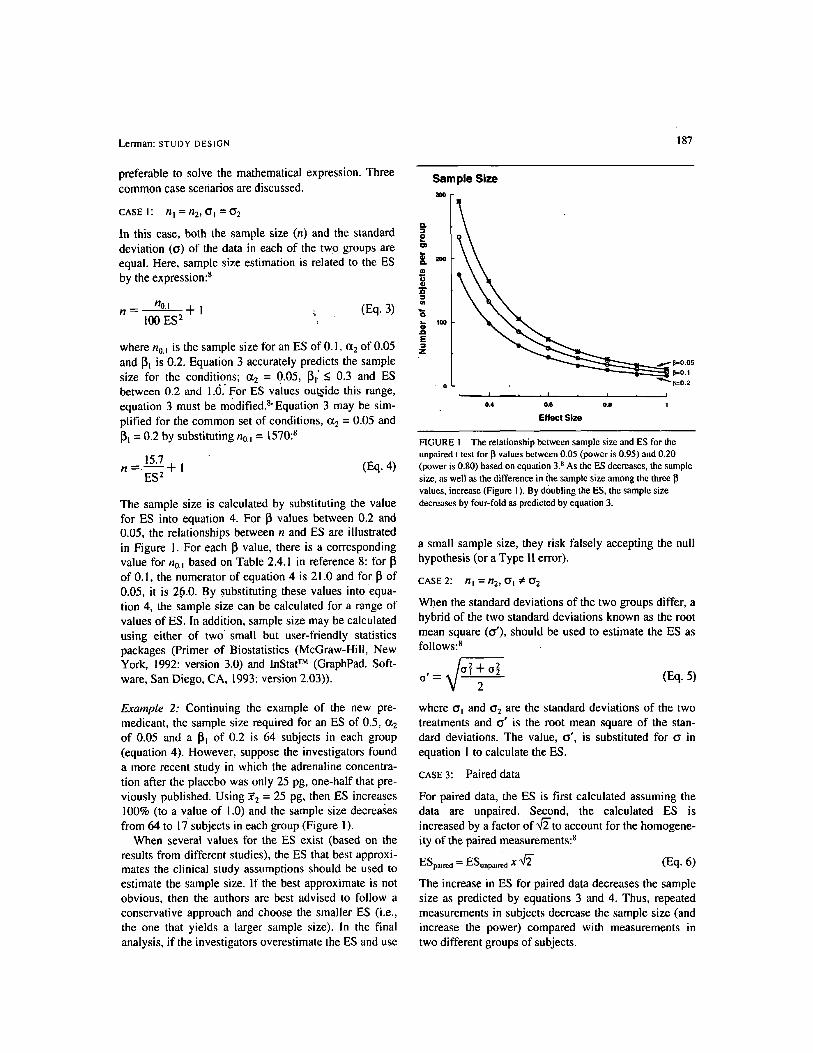
The sample size is calculated by substituting the value for ES into equation 4. For 13 values between 0.2 and 0.05, the relationships between n and ES are illustrated in Figure 1. For each ~ value, there is a corresponding value for n0. I based on Table 2.4.1 in reference 8: for I~ of 0.1, the numerator of equation 4 is 21.0 and for 13 of 0.05, it is 26.0. By substituting these values into equation 4, the sample size can be calculated for a range of values of ES. In addition, sample size may be calculated using either of two small but user-friendly statistics packages (Primer of Biostatistics (McGraw-Hill, New York, 1992: version 3.0) and InStat TM (GraphPad. Soft- ware, San Diego, CA, 1993: version 2.03)).

Example 2: Continuing the example of the new pre- medicant, the sample size required for an ES of 0.5, ~2 of 0.05 and a ~l of 0.2 is 64 subjects in each group (equation 4). However, suppose the investigators found a more recent study in which the adrenaline concentration after the placebo was only 25 pg, one-half that pre- viously published. Using ~2 = 25 pg, then ES increases 100% (to a value of 1.0) and the sample size decreases from 64 to 17 subjects in each group (Figure 1).

When several values for the ES exist (based on the results from different studies), the ES that best approximates the clinical study assumptions should be used to estimate the sample size. If the best approximate is not obvious, then the authors are best advised to follow a conservative approach and choose the smaller ES (i.e., the one that yields a larger sample size), in the final analysis, if the investigators overestimate the ES and use

187

Q .

o

- I

"6 JD E z

Sample Size 300

2OO

100

' 0

1~=0.05

~ 1~=0.1

~,=0.2

I I I I

0,4 0.6 0.8 1

Effect Size

FIGURE I The relationship between sample size and ES for the unpaired t test for I] values between 0.05 (power is 0.95) and 0.20 (power is 0.80) based on equation 3. s As the ES decreases, the sample size, as well as the difference in/he sample size among the three values, increase (Figure 1 ). By d()ubling the ES, the sample size decreases by four-fold as predicted by equation 3.

a small sample size, they risk falsely accepting the null hypothesis (or a Type I1 error).

CASE 2: nl = n2 ' a l :;6 O.2

When the standard deviations of the two groups differ, a hybrid of the two standard deviations known as the root mean square (a'), should be used to estimate the ES as follows: 8

2 + o 2 O ' ~ 2

(Eq. 5)

where o~ and o'2 are the standard deviations of the two treatments and o" is the root mean square of the standard deviations. The value, o' , is substituted for o. in equation I to calculate the ES.

CASE 3" Paired data

For paired data, the ES is first calculated assuming the data are unpaired. Second, the calculated ES is increased by a factor of ~ - t o account for the homogene- ity of the paired measurements: 8

EZpaired = ESunpaired x ~ (Eq. 6)

The increase in ES for paired data decreases the sample size as predicted by equations 3 and 4. Thus, repeated measurements in subjects decrease the sample size (and increase the power) compared with measurements in two different groups of subjects.

188

(b) PROPORTIONAL OR NOMINAL DATA - For proportional data, the estimate of the sample size is similar to that for parametric data with two exceptions. First, proportional data must be transformed (using the arcsine transformation) before simple mathematical operations can be performed. Second, the constant in equations 3 and 4, is omitted. Thus, the expression used to estimate the sample size for proportional data is: s

15.7 n - (Eq. 7)

h 2

for an ct2 = 0.05 and a 13~ = 0.2. The sample size may also be calculated using the mathematical expression in Appendix B. In addition, both the Primer of Biostatistics and Instat TM compute sample sizes for proportional data. However, all three of these techniques yield larger sample sizes than the equations of Cohen 8 (equation 7) as discussed below.

Example 3: Suppose the incidence of two events under consideration are: Pi (control) = 0.45 and P2 = 0.25. The arcsine transformation of Pi is 1.471 and of P2 is 1.0478. Using equation 2, "h" is 0.424. When this value is substituted into equation 7 together with an ct 2 of 0.05 and a 1~ of 0.2, a minimum of 88 subjects are required per group. Some statistics packages (Primer of Biostatistics and lnstat TM) may overestimate the sample size (by approximately 10%) compared with the size based on equation 7. However, the sample size estimates for proportions after Cohen 8 appear to be accurate, reliable and slightly smaller than values based on these other approaches.

Small differences in the sample size between treatments do not substantially decrease the power of the study, but large differences may. 8 When the size of one group is fixed (for example, only a limited number of subjects can receive an expensive new treatment) at a value that is far less than the sample size calculated for same size treatments, the size of the unfixed group must be increased disproportionately such that the total sample size exceeds the total for equal sized groups. 8,~~ Calculation of the sample size for unequal size groups uses equation 8 as follows:

n f X n n,, = (Eq. 8) 2nf - n

where n, is the unfixed sample size, n/is the fixed sample size and n is the sample size estimate for same size groups (as per equations 4 or 7). n/must be >0.5n, oth- erwise the denominator in equation 8 becomes negative or zero, thereby making equation 8 insoluble. If nf cannot be increased to solve equation 8, then o~, 13 or the ES

CANADIAN JOURNAL OF ANAESTHESIA

FIGURE 2 The sample size (ordinate axis) in a study in which the probability of an event in the treatment group (P2) is 50% that in the control group (PI). The control proportion (PI) is the probability that the event occurs in the control group, shown on the abscissa. The sample size estimates were based on oh = 0.05, and 13 = 0.20 and equation 7.

should be adjusted to decrease n. In example 2 with equal sample sizes, 64 subjects were required for each group or 128 subjects in total. However, if one sample size had been fixed (nf) to 35 subjects, then the unfixed sample size (nu) would require 375 subjects for the same o~, I~ and ES. In this case, the number of subjects increases to 410 or 3 fold the number with equal sample sizes.

When summarizing the sample size estimation, all of the assumptions used should be reported including the and I~ values, and the means and standard deviations or the estimated probabilities of the outcome events (i.e., proportions) (with the actual data or the sources of the data). When incomplete information is provided, it may be difficult to determine the assumptions used to calculate the sample size. For example, when the sample size is reported to be based on a 50% decrease in the incidence of an event in the treatment group compared with the control group, there is a whole range of sample sizes possible as shown in Figure 2. In this case, the actual incidence used in the calculation of the sample size should be reported. The summary of this information usually involves only a statement or two at the conclusion of the methods section to outline the details of how the sample size was estimated.

Lerman: S T U D Y D E S I G N 189

2 Power analysis If, after completion of a study, the null hypothesis is accepted, two possible scenarios may exist: (1) that the treatments have equipoise (or are similar) or (2) that the power of the study was inadequate to prove the treatments differed (Type II error). Before concluding that the treatments have equipoise, it is important to determine whether a statistically significant difference between the treatments could have been detected if the treatments truly differed.

The power of a study is the probability of correctly accepting the null hypothesis (1-13). Biological scien- tists have accepted a maximum value for IB of 0.2 or a power of 80%. Thus, when treatments are found to have equipoise, the null hypothesis may be falsely accepted if the power of the study is <80% or correctly accepted if the power is >80%. The power of a study is determined after completion of the study, using the actual sample size and ES and the o~ value. Power may be determined, for the same types of data as for the sample size calculation. Whenever the null hypothesis is accepted, a power analysis is warranted to validate the conclusions of the study. Power tables using the sample size and ES (calculated from the results of the study) as well as the o~ value are available in the standard textbooks.8

Example 4: Upon completion of a study in which 20 subjects were enrolled in each of two groups, the investigators concluded that two treatments had equipoise. The investigators had not performed a sample size calculation before undertaking the study. In this example, the ES was 0.5, o~ 2 was 0.05 and the sample size was 20. Using power tables, s the power of the study was only 33%, less than the minimum power of 80% required to correctly accept the null hypothesis. Based on this low power, the investigators could not conclude that the two treatments were similar, but rather that they were unable to detect a statistically significant difference between the treatments. On the basis of the results of this study, the investigators would have required 64 subjects in each treatment group to accept the null hypothesis with a power of 80%.

Several strategies may be considered in order to maximize the power of a study. 8.~~ First, the sample size in each treatment group should be similar. When the sample sizes are equal, the power of the study is maximal; as the difference between sample sizes increases, the power of the study decreases. Other strategies that increase the power include repeat measurements in the same subjects rather than singular measurements in several cohorts of subjects and measurement techniques that minimize the variability in the outcome variable

(i.e., minimizes the standard deviation of the measured variable). These strategies must be considered during the design phase of the study to maximize the power of the study.

When the null hypothesis is accepted at the conclusion of a study, some investigators dismiss the study as a failure because a statistically significant difference had not been achieved. However, such studies should not be dismissed frivolously. If the power of the study was sufficient to detect a clinically relevant difference between the treatments, then the treatments were similar and the results relevant to clinical practice. This study would merit publication. If the study had insufficient power to detect a clinically relevant difference, then the flawed study design also merits publication to serve as a guide to other investigators for future study designs. As the application of power analysis becomes widespread, the clinical relevance of studies in which the null hypothesis is accepted, will be enhanced.

Appendix A

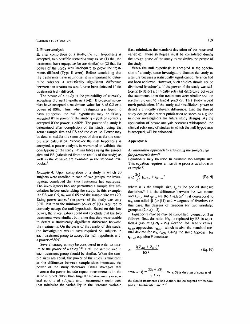
An alternative approach to estimating the sample size for parametric data t~ Equation 9 may be used to estimate the sample size. This equation requires an iterative process as shown in example 5.

> 2St2~ t 2 n _ 82 (t,(21,o+ 13(,.o) (Eq. 9)

where n is the sample size, st, is the pooled standard deviation,* 8 is the difference between the two means and ta(2),v and tl~(i)v are the t values I~ that correspond to a2, one-tailed IB (or IBl) and v degrees of freedom (in this case, the degrees of freedom for two unrelated groups = (2 x n) - 2).

Equation 9 may be may be simplified to equation 3 as follows: first, the ratio, $/s~,, is replaced by ES in equation 4 (assuming o~ = 02). Second, for large v values, tac2) v approaches/a(2).~, which is also the standard normal deviate for Gt 2, Za(2). Using the same approach for tl~(~), v, equation 9 becomes:

2(Z~(21 + Z~l~t)2 n = (Eq. I0)

ES 2

*Where s2p -SSI+SS2 Here, SS is the sum of squares of O I -F- o 2

the data in treatments i and 2 and v are the degrees of freedom (n-I) in treatments I and 2/0

190 C A N A D I A N J O U R N A L OF A N A E S T H E S I A

Third, substituting 1.96 for Z0.05(2) and 0.8416 for Z0.2tt) into the numerator of equation 10 yields the numerator of equation 4, 15.7. t~ Cohen also noted that for these (z2 and I~t values, the sample size must be adjusted upwards slightly to yield accurate estimates of the sample size. He increased the sample size by the addition of a constant, in this case, I, to give equation 4.

Example 5: To estimate the sample size (n) using equation 9, a series of iterations'(or repeated calculations) is required because the sample size estimate is also one of the assumptions that determines the t values on the right side of the equation. We begin by guessing a sample size (any guess is acceptable, although the most efficient solution is achieved by overestimating the first sample size) and determine the two t values (ta(2) and. tl~o)) that correspond to this first sample size using t tables, t~ These values, together with the sp and 5 are substituted into the right side of equation 9 to yield the first calculated sample size. The second estimate of the sample size is a value that lies between the first estimated and calculated sample sizes. Using this new estimate of n, two new t values are generated and substituted into equation 9. The second calculated sample size is compared with the second estimated sample size and the process continues until the estimated and calculated sample sizes converge.

Using the data from the premedication example, 5 is 25, c~ is 50, ~ = 0.05 and I~ = 0.2. Our first estimate of the sample size is 20 subjects per group. This corresponds to a v = 38, t0.05(2),38 = 2.024 and t0.2(t).38 = 0.851. ~t Substituting these values into equation 9 yields

2x(50)2 (2.024 + 0.851) 2 = 63.6. n - (25)--- S -

Our second estimate of the sample size is 60 subjects which corresponds to a v = I 18. In this case, to.05(2),tt 8 = 1.975 and to.2o),~18 = 0.845. Substituting these values yields an n = 63.8. Thus, our sample size should be at least 64 subjects. This value is consistent with the results of the example for CASE I.

Appendix B

An alternative approach to estimating the sample size for proportional data w

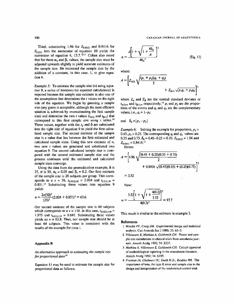
Equation 11 may be used to estimate the sample size for proportional data as follows:

n = 45h 2

(Eq. i l)

where:

A = [Z~(2, ~ / (p ' +Pg(q, + q ~ 2

+ Zp(u ~/Plq] +

q

J

where Za and Zp are the normal standard deviates or tat2),** and tp(~), respectively, t~ p~ and P2 are the proportions of the events and qt and q2 are the complementary values, i.e., q~ = l-pi:

and 5 h = l P l - P z l

Example 6: Solving the example for proportions, Pt = 0.45, P2 = 0.25. The corresponding ql and q2 values are 0.55 and 0.75.5h = 0.45-0.25 = 0.20. Zo.o5(2) = 1.96 and Zo.oso) = 0.8416. I I

Hence:

A = !.96 ~/(0.45 + 0.25)(0.55 + 0.75) 2

9 ] + 0.8416 x/(0.45)(0.55) + (0.25)(0.75)

= 3.52

Now:

+ 4(0.2)]2 3.52 I + I 3.52 /

J 97.7 n ~ 4(0.2) 2

This result is similar to the estimate in example 3.

References 1 Moodie PF, Craig DB. Experimental design and statistical

analysis. Can Anaesth Soc J 1986; 33: 63-5. 2 Villeneuve E, Mathieu A. Goldsmith CH. Power and sam-

ple size calculations in clinical trials from anesthesia jour- nals. Anesth Analg 1992; 74: $337.

3 Mathieu A, Villeneuve E, Goldsmith CH. Critical appraisal of methodological reporting in the anaesthesia literature. Anesth Analg 1992; 74: S195.

4 Freiman JA, Chalmers TC, Smith H Jr., Keubler RR. The importance of beta, the type I! error and sample size in the design and interpretation of the randomized control trial.

Lerman: STUDY DESIGN 191

Survey of 71 "negative" trials. N Engl J Med 1978; 299: 690-4.

5 Gardner M J, Bond J. An exploratory study of statistical assessment of papers published in the British Medical Journal. JAMA 1990; 263:1355-7

6 Fisher DM. Statistics in Anesthesia. In: Anesthesia. Miller RD (ed.). 4th ed. New York: Churchill Livingstone, 1994: 782-5

7 Cohen J. The statistical power of abnormal social psycho- logical research: a review. J Abnorm Soc Psychol 1962; 65: 145-53.

8 Cohen J. Statistical Power Analysis for the Behavioural Sciences. 2nd ed. Hillsdale, New Jersey: Lawrence Erlbaum Associates, 1988: 1-74,179-213

9 Glantz SA. Primer of Biostatistics. 3rd ed. New York: McGraw-Hill, 1992: 91-4, 133-8, 387

I 0 Zar JH. Biostatistical Analysis. 2nd ed. Englewood Cliffs: Prentice-Hall, Inc., 1984: 134-7, 171-6, 397-400, 484-5, 586-8

I 1 Snedecor GW, Cochran WG. Statistical Methods. 7th ed. Ames, Iowa: The Iowa State University Press, 1980: 469.

statistics study design in clinical research: sample size estimation and power ... · 184...

Documents