Statistics Review Part 1

Random Variables and their Distributions

Random Variables

• random variables (RV) are variables whose outcome is subject to chance. – That is, we don’t know what value the variable will take until we

observe it. Examples:• Outcome of a coin toss; roll of a die; sum of two dice.• Value of the S&P 500 one year from today. • Value of the S&P 500 one year from today. • Starting salary at your first job after graduation.

• The actual value taken by a RV is called an outcome.• Usually, we'll use capital letters to denote a random variable,

and lower case letters to denote a particular outcome.– Example: rolling two dice. Call the sum of the values rolled X. A

particular outcome might be x = 7.

Discrete vs. Continuous RV’s

• Random variables are said to be discrete if they can only take on a finite (or countable) set of values.– Outcome of a coin toss: {Heads, Tails}

– Outcome of rolling a die: {1, 2, 3, 4, 5, 6}

– Gender of the next person you meet: {Male, Female}

• Random variables are said to be continuous if they take on a continuum (uncountable infinity) of values.– height of a person

– Starting salary at your first job after graduation

Probability

• Associated with every possible outcome of a RV is a probability. The probability of a particular outcome tells us how likely that outcome is.

• Pr(X = x) denotes the probability that random variable Xtakes value x. You can think of Pr(X = x) as the proportion of the time that outcome x occurs in the “long run” (in many takes value x. You can think of Pr(X = x) as the proportion of the time that outcome x occurs in the “long run” (in many repeated trials).

• Examples– For a coin toss, Pr(X=heads)=Pr(X=tails)=0.5 (or, 50%).– for a pair of dice whose sum is X, Pr(X=7)=0.167 (or,

16.7%, or 1/6). (Try it with a hundred dice rolls.)

Properties of Probabilities• Probabilities are numbers• Probabilities are between 0 and 1.• If Pr(X = x) = 0,

– then outcome X = x never occurs.– eg, sum of 2 dice roll: x=13

• If Pr(X = x) = 1,– then outcome X = x always occurs.– then outcome X = x always occurs.

• If two outcomes x,y are mutually exclusive (meaning x and y cannot both occur at the same time) then:

– Pr(X = x and X = y) = 0– Pr(X = x or X = y) = Pr(X = x) + Pr(X = y)– eg, sum of 2 dice roll: Pr(X=7 or X=8)=Pr(X=7)+Pr(X=8)=0.167+0.139=0.306

• If two outcomes x,y are mutually exclusive and collectively exhaustive (meaning no other outcomes are possible) then:

– Pr(X = x or X = y) = Pr(X = x) + Pr(X = y) = 1– eg, coin toss: x=heads, y=tails

Probability Distributions

• Every RV has a probability distribution. • A probability distribution describes the set of all possible outcomes of a

RV, and the probabilities associated with each possible outcome.• This is summarized by a function, called a probability distribution

function (pdf).function (pdf).• For a discrete RV, the pdf is just a list of all possible outcomes, and the

probability that each one occurs.• Example: coin toss

– Pr(X = heads) = Pr(X = tails) = ½• Example: rolling a single die

– Pr(X = 1) = Pr(X = 2) = ... = Pr(X = 6) = 1/6Note: in each case, the sum of probabilities of all possible outcomes is 1.

Cumulative Probability Distribution

• An alternate way to describe a probability distribution is the cumulative distribution function (cdf).

• The cdf gives the probability that a RV takes a value less than or equal to a given value, i.e., Pr(X ≤ x)

(Draw a picture)

Outcome (value of roll of single die)

1 2 3 4 5 6

pdf 1/6 1/6 1/6 1/6 1/6 1/6

cdf 1/6 1/3 1/2 2/3 5/6 1

Sum of Two Dice

Die A Value

Die BValue

1 2 3 4 5 6

1 2 3 4 5 6 7

2 3 4 5 6 7 82 3 4 5 6 7 8

3 4 5 6 7 8 9

4 5 6 7 8 9 10

5 6 7 8 9 10 11

6 7 8 9 10 11 12

Two Dice derive table (and figure) of pdf and cdf, in 36ths

2 3 4 5 6 7 8 9 10 11 12

pdf 1 2 3 4 5 6 5 4 3 2 1pdf 1 2 3 4 5 6 5 4 3 2 1

cdf 1 3 6 10 15 21 26 30 33 35 36

The case of continuous RVs• Because continuous RVs can take an infinite number of values, the

pdf and cdf can’t enumerate the probabilities of each of them.• Instead, we typically describe the pdf and cdf using functions.• For the pdf of a continuous RV, the “d” stands for “density”

instead of “distribution” (this is a technical point)• Usual notation for the pdf is f(x)• Usual notation for the pdf is f(x)• Usual notation for the cdf is F(x) = Pr(X ≤ x)• Example, the uniform distribution over [0,1]: f(x)=1; F(x)=x.• Example: the normal distribution:

(draw them)

( )

( )∫∞

∞−=

−−=

dttfxF

xxf

)(

2exp

2

1)(

2

2

2 σµ

πσ

Graphing pdfs and cdfs of continuous RVs

• Because pdfs and cdfs of continuous RVs can be complicated functions, in this class we’ll just use pictures to represent them

• For both, we plot outcomes (i.e., x) on the horizontal axis, and probabilities (i.e., f(x) or F(x)) on the vertical axis

• Since probabilities are weakly positive, the pdf is weakly positive, and the cdf is a weakly increasing function.

• Since probabilities are weakly positive, the pdf is weakly positive, and the cdf is a weakly increasing function.

• The cdf ranges from zero to one• The pdf typically has both increasing and decreasing segments

– The area under the pdf gives the probability that X falls in an interval

– Hence the total area under the pdf must be one

• (draw some pictures: two dice, normal pdf & cdf, tail & interval probabilities)

Describing RVs

• There are lots of ways to describe the behavior of a RV

• Obviously, the pdf and cdf do this– in fact, they tell us “everything” we might want to know

about a RVabout a RV

• But sometimes we only want to describe one or two features of a probability distribution

• One feature of interest is the expected value (or mean) or a RV

• Another is a measure of the dispersion of the RV (how “spread out” the possible values are, e.g., the variance)

Expected Values

• Think of the expected value (or mean) of a RV as the long-run average value of the RV over many repeated trials

• You can also think of it as a measure of the “middle” of a probability distribution, or a “good guess” of the value of a RV

• Denoted E(X) or µX• Denoted E(X) or µX

• More precisely, E(X) is a probability-weighted average of all possible outcomes of X

• Example: rolling a die– f(1) = f(2) = f(3) = f(4) = f(5) = f(6) = 1/6– E(X) = 1*(1/6) + 2*(1/6) + 3*(1/6) + 4*(1/6) + 5*(1/6) + 6*(1/6)

= 1/6 + 2/6 + 3/6 + 4/6 + 5/6 + 6/6= 21/6 = 3.5

• interpretation?

More about E(X)

• The general case for a discrete RV– Suppose RV X can take k possible values x1, x2, ... , xk with

associated probabilities p1, p2, ... , pk then

∑=k

ii xpXE )(

• The general case for a continuous RV involves an integral

• We can think of E(X) as a mathematical operator (like +, -, *, /).– It is a linear operator, which means we can pass it through

addition and subtraction operators

– That is, if a and b are constants and X is a RV,E(a + bX) = a + bE(X)

∑=

=i

ii xpXE1

)(

Variance & Standard Deviation• The variance and standard deviation measure dispersion, or how “spread out” a

probability distribution is.• A large variance means a RV is likely to take a wide range of values• A small variance means a RV is likely to take a narrow range of values. That is,

likely values are clustered together• Denoted Var(X) or • Formally, if RV X takes one of k possible values x1, x2, ... ,xk

2Xσ

1 2 k

• Note: Var(X) = E[(x - µX)2] ≠ [E(x - µX)]2 (why?)• Because Var(X) is measured on an awkward scale (the square of the scale of X),

we often prefer the standard deviation of X:

which is measured on the same scale as X• A useful formula: Var(a + bX) = b2Var(X)

( )[ ] ( )∑=

−=−=k

iXiiX xpXEXVar

1

22)( µµ

)(XVarX =σ

Variance & Standard Deviation Example: a single die

• Example: variance of rolling a die– Recall f(1) = f(2) = f(3) = f(4) = f(5) = f(6) = 1/6 and E(X) = 3.5– Var(X) = (1 – 3.5)2/6 + (2 – 3.5)2/6 + (3 – 3.5)2/6 + (4 – 3.5)2/6

+ (5 – 3.5)2/6 + (6 – 3.5)2/6≈ 2.92

– σ ≈ 1.71– σX ≈ 1.71

Samples and Population

• A random variable’s probability distribution, expected value, and variance exist on an abstract level.

• They are population quantities (we’ll define this soon).• That is, we don’t generally know what a random

variable’s pdf/cdf is, nor do we know its expected value variable’s pdf/cdf is, nor do we know its expected value or variance.

• As econometricians, our goal is to estimate these quantities.

• We do that by computing statistics from a sample of data drawn from the population.

• Our goal as econometricians is ALWAYS to learn about a population from sample information.

Two Random Variables

• Most interesting questions in economics involve 2 (or more) variables– what’s the relationship between education and earnings?

– what’s the relationship between stock price and profits?

• We describe the probabilistic relationship between two (or more) random variables using three kinds of probability distributions:– the joint distribution

– marginal distributions

– conditional distributions

The Joint Distribution

• The joint distribution of discrete RVs X and Y is the probability that the two RVs simultaneously take on certain values, say x and y: That is, Pr(X = x, Y = y), like a cross-tab.

• Example: weather and commuting time.– Let C denote commuting time. Suppose commuting time can be long – Let C denote commuting time. Suppose commuting time can be long

(C = 1) or short (C = 0).

– Let W denote weather. Suppose weather can be fair (W = 1) or foul (W = 0).

– There are four possible outcomes: (C = 0, W = 0), (C = 0, W = 1), (C = 1, W = 0), (C = 1, W = 1).

– The probabilities of each outcome define the joint distribution of C and W:

Foul Weather (W=0) Fair Weather (W=1) Total

Short Commute (C=0) 0.15 0.25 0.4

Long Commute (C=1) 0.55 0.05 0.6

Total 0.7 0.3 1

Marginal Distributions

• When X,Y have a joint distribution, we use the term marginal distribution to describe the probability distribution of X or Y alone.

• We can compute the marginal distribution of X from the joint distribution of X,Y by adding up the probabilities of all possible outcomes where X takes a particular value. That is, if Y takes one of kpossible values: ( )∑ ====

k

yYxXxX ,Pr)Pr(possible values:

The marginal distribution of weather is in blue. The marginal distribution of commuting time is in yellow.

( )∑=

====i

iyYxXxX1

,Pr)Pr(

Foul Weather (W=0) Fair Weather (W=1) Total

Short Commute (C=0) 0.15 0.25 0.4

Long Commute (C=1) 0.55 0.05 0.6

Total 0.7 0.3 1

Conditional Distributions

• The distribution of a random variable Y conditional on another random variable X taking a specific value is called the conditional distribution of Y given X.

• The conditional probability that Y takes value y when Xtakes value x is written Pr(Y = y | X = x).takes value x is written Pr(Y = y | X = x).

• In general,

• Intuitively, this measures the probability that Y = y and X=x, given that X = x.– Example: what’s the probability of a long commute, given that

the weather is foul? (Next slide)

)Pr(),Pr(

)|Pr(xX

xXyYxXyY

======

Example: Commuting Time

• What’s the probability of a long commute (C = 1) given foul

Foul Weather (W=0) Fair Weather (W=1) Total

Short Commute (C=0) 0.15 0.25 0.4

Long Commute (C=1) 0.55 0.05 0.6

Total 0.7 0.3 1

• What’s the probability of a long commute (C = 1) given foul weather (W = 0)?

• We know the joint probability is Pr(C = 1, W = 0) = 0.55• The (marginal) probability of foul weather is Pr(W = 0) = 0.7 (this

is Vancouver, after all)• So given that the weather is foul, the probability of a long

commute is

Pr(C = 1 | W = 0) = Pr(C = 1, W = 0) / Pr(W = 0) = 0.55 / 0.7 ≈ 0.79

• Notice that Pr(C = 1 | W = 0) + Pr(C = 0 | W = 0) = 1. why?

Conditional Expectation• The mean of the conditional distribution of Y given X is called the

conditional expectation (or conditional mean) of Y given X.• It’s the expected value of Y, given that X takes a particular value.• It’s computed just like a regular (unconditional) expectation, but

uses the conditional distribution instead of the marginal.– If Y takes one of k possible values y1, y2, ... , yk then:

k– If Y takes one of k possible values y1, y2, ... , yk then:

• Example: in our commuting example, suppose a long commute takes 45 minutes and a short commute takes 30 minutes. What’s the expected length of the commute, conditional on foul weather? What if weather is fair?– Foul weather: 30*0.15/0.7 + 45*0.55/0.7 = 41.79 minutes– Fair weather: 30*0.25/0.3 + 45*0.05/0.3 = 32.5 minutes

( ) ( )∑=

====k

iii xXyYyxXYE

1

|Pr|

The Law of Iterated Expectations

• There is a simple relationship between conditional and unconditional expectations. We call it the law of iterated expectations.

• Intuitively, an unconditional expectation is just a weighted average of conditional expectations where the weights are the probabilities of the outcomes on which weighted average of conditional expectations where the weights are the probabilities of the outcomes on which we are conditioning.– Example: the mean height of adults in Canada is a weighted

average of the mean height of men and the mean height of women, where the weights are the proportions of men and women in the population.

– Example: the mean (expected) commuting time is just a weighted average of the mean (expected) commuting time in foul weather and the mean (expected) commuting time in fair weather. Here, the weights are the probabilities of foul and fair weather, respectively.

The Law of Iterated Expectations, continued

• Formally, for a RV Y and discrete RV X that takes one of mpossible values, the law of iterated expectations is:

• More generally: E(Y) = E[E(Y|X)]

( ) ( ) ( )∑=

===m

iii xXxXYEYE

1

Pr|

• More generally: E(Y) = E[E(Y|X)]• THIS IS A VERY USEFUL RESULT!!• Back to the commuting time example:

– E(commuting time) = E(commuting time | foul weather)*Pr(foul weather)

+ E(commuting time | fair weather)*Pr(fair weather)= 41.79* 0.7 + 32.5*0.3 = 39 minutes

Conditional Variance

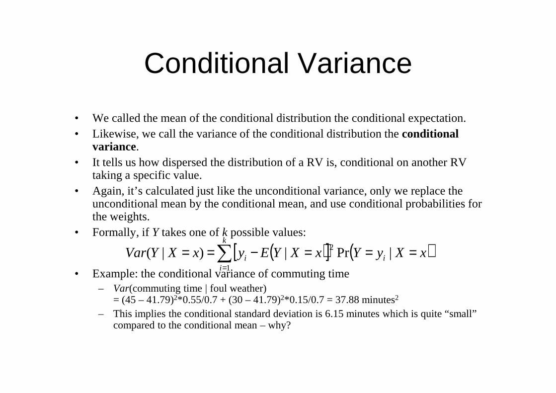
• We called the mean of the conditional distribution the conditional expectation.• Likewise, we call the variance of the conditional distribution the conditional

variance.• It tells us how dispersed the distribution of a RV is, conditional on another RV

taking a specific value. • Again, it’s calculated just like the unconditional variance, only we replace the • Again, it’s calculated just like the unconditional variance, only we replace the

unconditional mean by the conditional mean, and use conditional probabilities for the weights.

• Formally, if Y takes one of k possible values:

• Example: the conditional variance of commuting time– Var(commuting time | foul weather)

= (45 – 41.79)2*0.55/0.7 + (30 – 41.79)2*0.15/0.7 = 37.88 minutes2

– This implies the conditional standard deviation is 6.15 minutes which is quite “small” compared to the conditional mean – why?

( )[ ] ( )∑=

===−==k

iii xXyYxXYEyxXYVar

1

2 |Pr|)|(

Independence

• Quite often, we’re interested in quantifying the relationship between two RVs.– In fact linear regression methods (the focus of this course) do exactly this.

• When two RVs are completely unrelated, we say they are independently distributed (or simply independent).– If knowing the value of one RV (say X) provides absolutely no information

about the value of another RV (say Y), we say that X and Y are independent.about the value of another RV (say Y), we say that X and Y are independent.• Formally, X and Y are independent if the conditional distribution of Y given

X equals the marginal distribution of Y:

Pr(Y = y | X = x) = Pr(Y = y) (*)

• Equivalently, X and Y are independent if the joint distribution of X and Yequals the product of their marginal distributions:

Pr(Y = y, X = x) = Pr(Y = y)Pr(X = x)– This follows immediately from (*) and the definition of the conditional

distribution:

)Pr(

),Pr()|Pr(

xX

yYxXxXyY

======

Covariance

• A very common measure of association between two RVs is their covariance. It is a measure of the extent to which to RVs “move together.”

• Cov(X,Y) = σXY = E[(X – µX)(Y – µY)]• In the discrete case, if X takes one of m values and Y takes one of k

values, we have( )( ) ( )∑∑

k mvalues, we have

• Interpretation: – if X and Y are positively correlated (σXY > 0) then when X > µX we also have Y > µY, and when X < µX we also have Y < µY (in expectation). This means X and Ytend to move “in the same direction.”

– Conversely, if σXY < 0 then when X > µX we have Y < µY, and when X < µX we have Y > µY (in expectation). This means X and Y tend to move “in opposite directions.”

( )( ) ( )∑∑= =

==−−=k

i

m

jijYiXj yYxXyxYXCov

1 1

,Pr),( µµ

A Caveat

• Note: if σXY = 0, this does not mean that X and Y are independent (except in the special case where X and Y are both normally distributed).

• However, the converse is true: if X and Y are independent, then σ = 0.independent, then σXY = 0.

• This tells us that independence is a “stronger” property than zero covariation.

• covariance is only a measure of linearassociation – so X and Y can have an exactnonlinear relationship and zero covariance.

Covariance and Correlation

• An unfortunate property of the covariance measure of association is that it is difficult to interpret: it is measured in units of X times units of Y.

• A “unit free” measure of association between to RVs is the correlation between X and Y: correlation between X and Y:

– Notice that the numerator & denominator units cancel.

• Corr(X,Y) lies between -1 and 1.

• If Corr(X,Y) = 0 then we say X and Y are uncorrelated.

• Note that if Cov(X,Y) = 0 then Corr(X,Y) = 0 (and vice versa).

( ) ( )( ) ( ) YX

XYXY

YVarXVar

YXCovYXCorr

σσσρ === ,

,

Example: Weather and Commuting Time

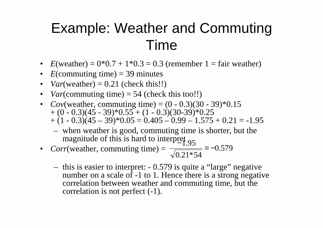
• E(weather) = 0*0.7 + 1*0.3 = 0.3 (remember 1 = fair weather)• E(commuting time) = 39 minutes• Var(weather) = 0.21 (check this!!)• Var(commuting time) = 54 (check this too!!)• Cov(weather, commuting time) = (0 - 0.3)(30 - 39)*0.15

+ (0 - 0.3)(45 - 39)*0.55 + (1 - 0.3)(30-39)*0.25+ (0 - 0.3)(45 - 39)*0.55 + (1 - 0.3)(30-39)*0.25+ (1 - 0.3)(45 – 39)*0.05 = 0.405 – 0.99 – 1.575 + 0.21 = -1.95 – when weather is good, commuting time is shorter, but the

magnitude of this is hard to interpret• Corr(weather, commuting time) =

– this is easier to interpret: - 0.579 is quite a “large” negative number on a scale of -1 to 1. Hence there is a strong negative correlation between weather and commuting time, but the correlation is not perfect (-1).

579.054*21.0

95.1 −=−

Some Useful Formulae

• Suppose that X, Y, and V are RVs and a, b, and c are constants. Then:

( )( )

( )XYYX

YX

abbabYaXVar

cbacYbXaE

σσσµµ

++=+

++=++

22222( )( )

( )( ) YXXY

VYXY

YY

XYYX

XYE

cbYcVbXaCov

YE

abbabYaXVar

µµσσσ

µσσσσ

+=+=++

+=

++=+

,

2222