statistics of contingency tables - hofroe.net · contingency tables stat 557 heike hofmann. outline...

Statistics of Contingency Tables

stat 557Heike Hofmann

Outline

• Summary Statistics:Difference of Proportions, Relative Risk, Odds, Odds Ratio

• Visualizations: Mosaicplots

• Concordance & Discordance

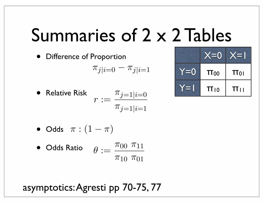
• Difference of Proportion

• Relative Risk

• Odds

• Odds Ratio

X=0 X=1

Y=0

Y=1

π00 π01

π10 π11

asymptotics: Agresti pp 70-75, 77

Summaries of 2 x 2 Tables

σ2(γ̂)∞ =16

n(ΠC + ΠD)4

I�

i=1

J�

j=1

πij

�ΠCπd

ij −ΠDπcij

�2

γ =ΠC −ΠD

ΠC + ΠD

θ :=π00 π11

π10 π01

π : (1− π)

πj|i=0 − πj|i=1 =: π1 − π2,

r :=πj=1|i=0

πj=1|i=1

χ21,0.05 = 3.84, χ2

1,0.01 = 6.634897

πij = πi+ · π+j

Ho : P ( heart disease | Cholesterol ≤ 220) =P ( heart disease | Cholesterol > 220)

π11

π11 + π12=

π21

π21 + π22

Let X, Y be two categorical variables, with I, J categories respectively and X ∈ {x1, x2, ..., xI}, Y ∈{y1, y2, ..., yJ}.

Then the pair (X, Y ) is categorical variable with IJ outcomes.The table

X\Y y1 y2 ... yJ

x1 n11 n12 ... n1J n1.

x2 n21 n22 ... n2J n2....

...... . . . ...

...xI nI1 nI2 ... nIJ nI.

n.1 n.2 ... n.J n

2

σ2(γ̂)∞ =16

n(ΠC + ΠD)4

I�

i=1

J�

j=1

πij

�ΠCπd

ij −ΠDπcij

�2

γ =ΠC −ΠD

ΠC + ΠD

θ :=π00 π11

π10 π01

π : (1− π)

πj|i=0 − πj|i=1 =: π1 − π2,

r :=πj=1|i=0

πj=1|i=1

χ21,0.05 = 3.84, χ2

1,0.01 = 6.634897

πij = πi+ · π+j


π11

π11 + π12=

π21

π21 + π22



X\Y y1 y2 ... yJ

x1 n11 n12 ... n1J n1.

x2 n21 n22 ... n2J n2....

...... . . . ...


n.1 n.2 ... n.J n

2

σ2(γ̂)∞ =16

n(ΠC + ΠD)4

I�

i=1

J�

j=1

πij

�ΠCπd

ij −ΠDπcij

�2

γ =ΠC −ΠD

ΠC + ΠD

θ :=π00 π11

π10 π01

π : (1− π)

πj|i=0 − πj|i=1 =: π1 − π2,

r :=πj=1|i=0

πj=1|i=1

χ21,0.05 = 3.84, χ2

1,0.01 = 6.634897

πij = πi+ · π+j


π11

π11 + π12=

π21

π21 + π22



X\Y y1 y2 ... yJ

x1 n11 n12 ... n1J n1.

x2 n21 n22 ... n2J n2....

...... . . . ...


n.1 n.2 ... n.J n

2

gk(T ) =eTk

�K�=1 eT�

σ(ν) =1

1 + e−ν

Zm = σ(α0m + α�mX) m = 1, ...,M

Tk = β0k + β�kZ k = 1, ...,K

fk(X) = gk(T ) k = 1, ...,K

Πc = 2I�

i=1

J�

j=1

πij ·�

h>i

�

k>j

πhk =�

i,j

πcij

σ2(γ̂)∞ =16

n(ΠC + ΠD)4

I�

i=1

J�

j=1

πij

�ΠCπd

ij −ΠDπcij

�2

γ =ΠC −ΠD

ΠC + ΠD

θ :=π00 π11

π10 π01

π : (1− π)

πj|i=0 − πj|i=1 =: π1 − π2,

r :=πj=1|i=0

πj=1|i=1

χ21,0.05 = 3.84, χ2

1,0.01 = 6.634897

πij = πi+ · π+j


π11

π11 + π12=

π21

π21 + π22

2

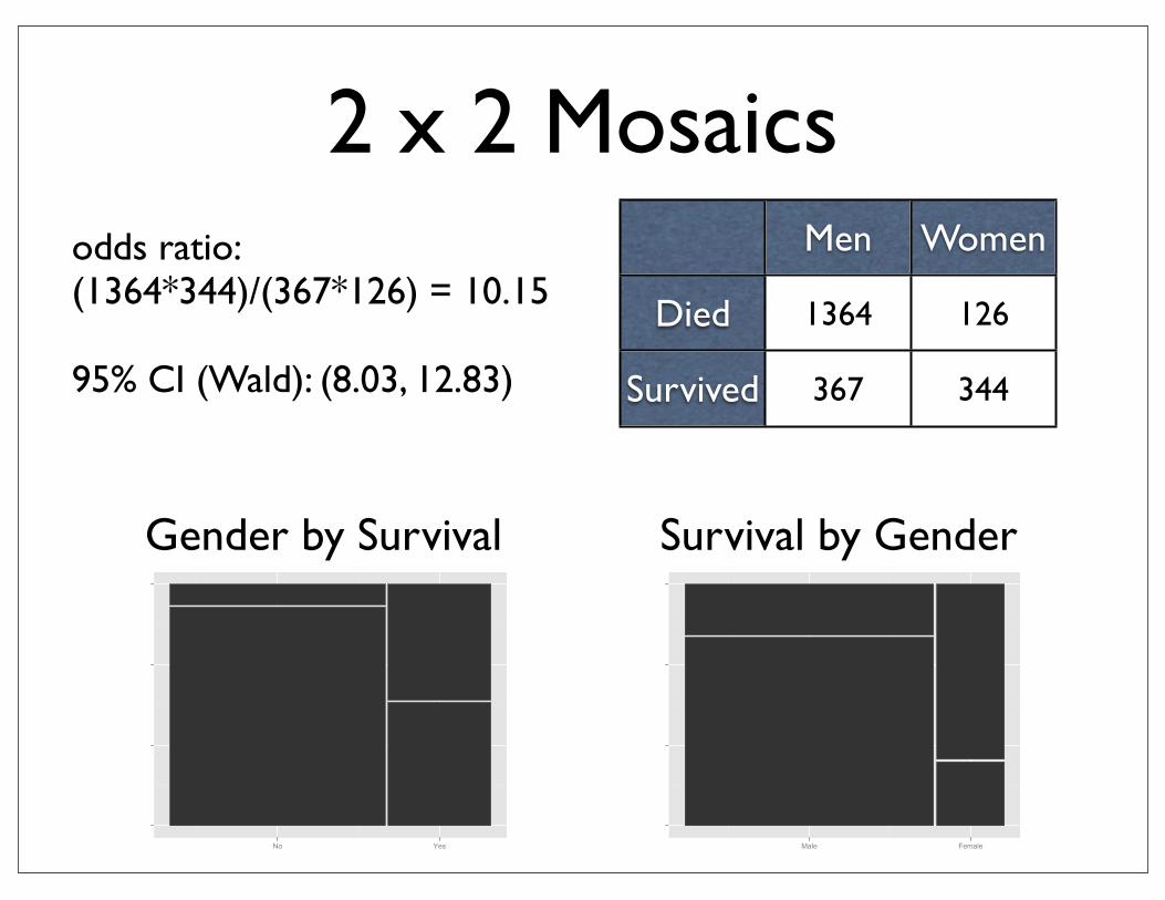
2 x 2 Mosaicsodds ratio: (1364*344)/(367*126) = 10.15

95% CI (Wald): (8.03, 12.83)

Men Women

Died

Survived

1364 126

367 344

No Yes Male Female

Gender by Survival Survival by Gender

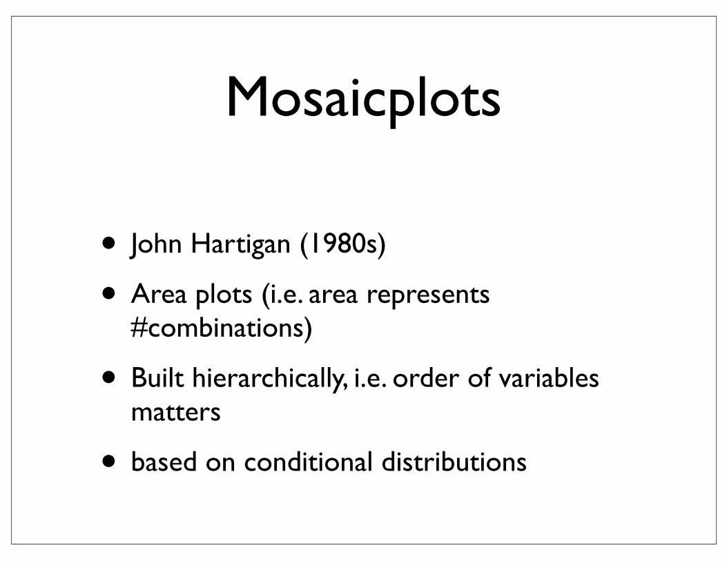
• John Hartigan (1980s)

• Area plots (i.e. area represents #combinations)

• Built hierarchically, i.e. order of variables matters

• based on conditional distributions

Mosaicplots

Mosaicplots

No Yes Male Female

P(X,Y)

P(X|Y)*P(Y) P(Y|X)*P(X)

prodplot(tc, Freq~Sex+Survived, c("vspine", "hspine"), subset=level==2)

prodplot(tc, Freq~Survived+Sex, c("vspine", "hspine"), subset=level==2)

= =

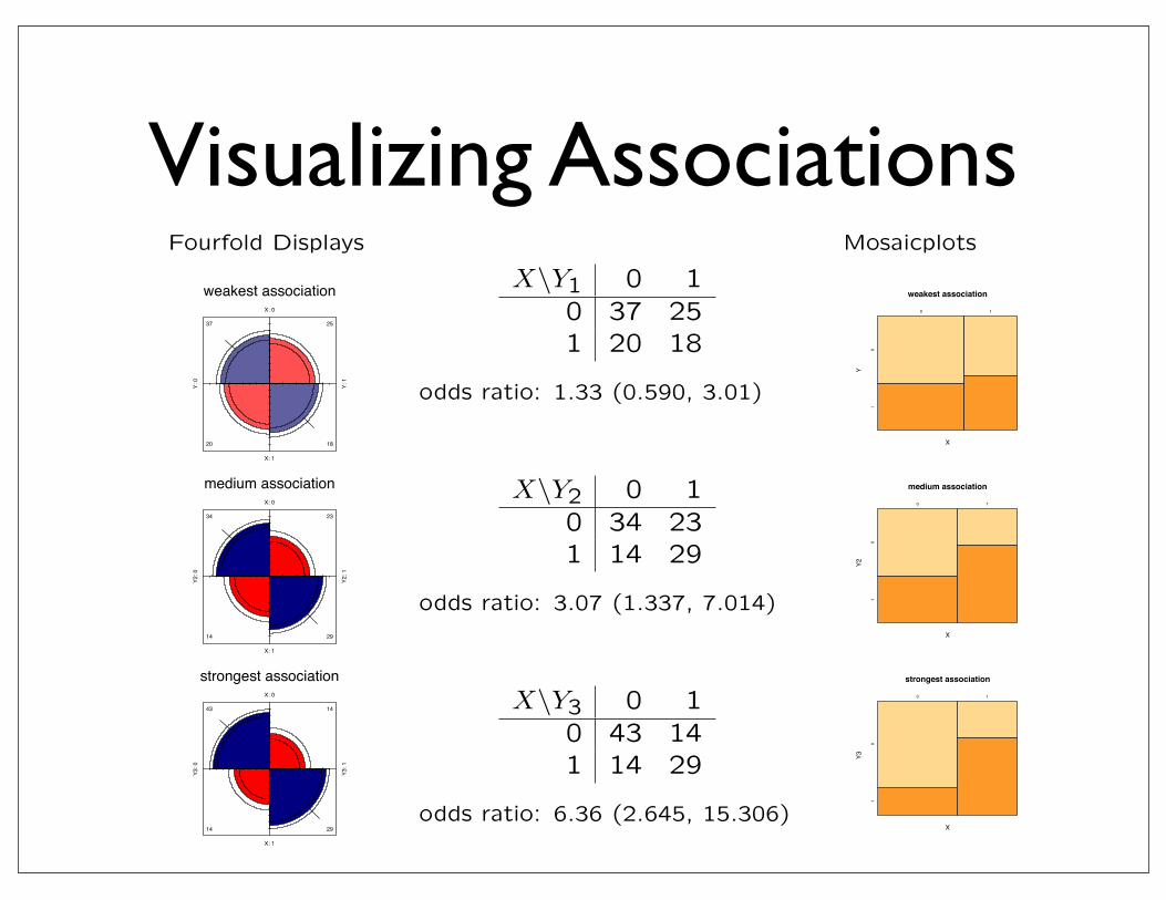
Visualizing AssociationsVisualizing Associations - 2 x 2 tables

Fourfold Displays

X: 0

Y:

0

X: 1

Y:

1

37

20

25

18

weakest association

X: 0

Y2

: 0

X: 1

Y2

: 1

34

14

23

29

medium association

X: 0

Y3

: 0

X: 1

Y3

: 1

43

14

14

29

strongest association

X\Y1 0 10 37 251 20 18

odds ratio: 1.33 (0.590, 3.01)

X\Y2 0 10 34 231 14 29

odds ratio: 3.07 (1.337, 7.014)

X\Y3 0 10 43 141 14 29

odds ratio: 6.36 (2.645, 15.306)

Mosaicplots

weakest association

X

Y

0 1

01

medium association

X

Y2

0 1

01

strongest association

X

Y3

0 1

01

Interface/CSNA ’05 Mosaics for Association Models [email protected]

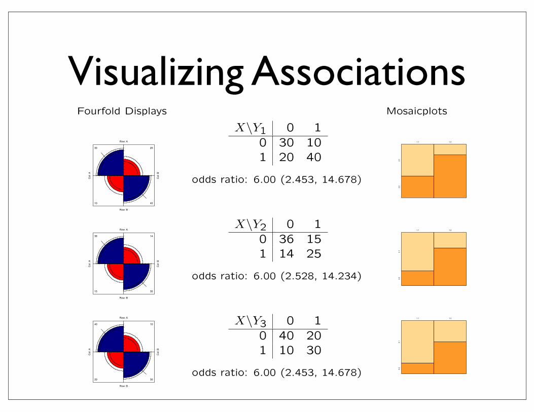
Visualizing AssociationsVisualizing Associations - 2 x 2 tables

Fourfold Displays

Row: A

Co

l: A

Row: B

Co

l: B

30

10

20

40

Row: A

Co

l: A

Row: B

Co

l: B

36

15

14

35

Row: A

Co

l: A

Row: B

Co

l: B

40

20

10

30

X\Y1 0 10 30 101 20 40

odds ratio: 6.00 (2.453, 14.678)

X\Y2 0 10 36 151 14 25

odds ratio: 6.00 (2.528, 14.234)

X\Y3 0 10 40 201 10 30

odds ratio: 6.00 (2.453, 14.678)

Mosaicplots

1.1 1.2

2.1

2.2

1.1 1.2

2.1

2.2

1.1 1.2

2.1

2.2

Interface/CSNA ’05 Mosaics for Association Models [email protected]

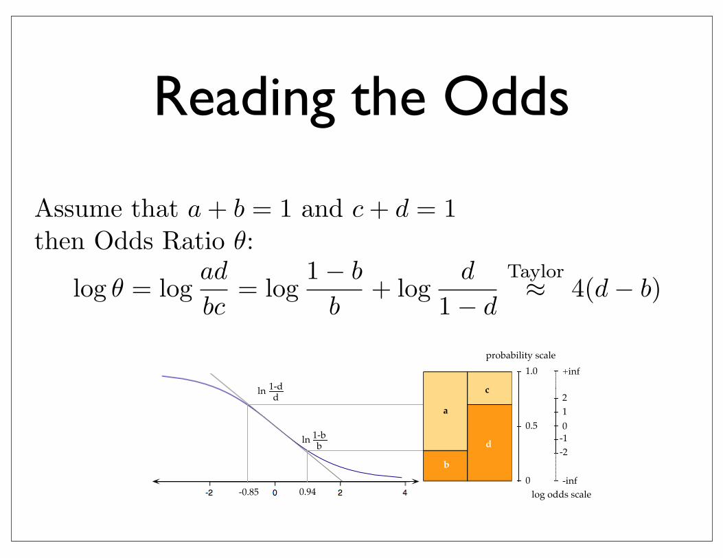
Reading the Odds

0.94

1-bbln

1-ddln

-0.85

+inf

0

-inf

2

-2-1

1

log odds scale

0.5

probability scale

0

1.0

b

a

d

c

Assume that a + b = 1 and c + d = 1

then Odds Ratio θ:

log θ = logad

bc= log

1− b

b+ log

d

1− d

Taylor≈ 4(d− b)

p̃ =y + 2

n + 4

p̃ ± zα/2

�1

np̃(1− p̃)

p− po�1npo(1− po)

= ±zα/2

p +

z2α/2

2n± zα/2

��

p(1− p) +

z2α/2

4n

�/n

�

1 +

z2α/2

n

�−1

p =Y

n

|p− π|�1np(1− p)

.∼ N(0, 1)

nπ ≥ 5, n(1− π) ≥ 5

λ ·��

β2+

�α2

�

{α0m, αm : m = 1, ...,M} M(p + 1)

{β0k, βk : k = 1, ...,K} K(M + 1)

gk(T ) =eTk

�K�=1 eT�

σ(ν) =1

1 + e−ν

Zm = σ(α0m + α�mX) m = 1, ...,M

Tk = β0k + β�kZ k = 1, ...,K

fk(X) = gk(T ) k = 1, ...,K

1


then Odds Ratio θ:

log θ = logad

bc= log

1− b

b+ log

d

1− d

Taylor≈ 4(d− b)

p̃ =y + 2

n + 4

p̃ ± zα/2

�1

np̃(1− p̃)


= ±zα/2

p +

z2α/2

2n± zα/2

��

p(1− p) +

z2α/2

4n

�/n

�

1 +

z2α/2

n

�−1

p =Y

n

|p− π|�1np(1− p)

.∼ N(0, 1)

nπ ≥ 5, n(1− π) ≥ 5

λ ·��

β2+

�α2

�

{α0m, αm : m = 1, ...,M} M(p + 1)

{β0k, βk : k = 1, ...,K} K(M + 1)

gk(T ) =eTk

�K�=1 eT�

σ(ν) =1

1 + e−ν

Zm = σ(α0m + α�mX) m = 1, ...,M

Tk = β0k + β�kZ k = 1, ...,K

fk(X) = gk(T ) k = 1, ...,K

1

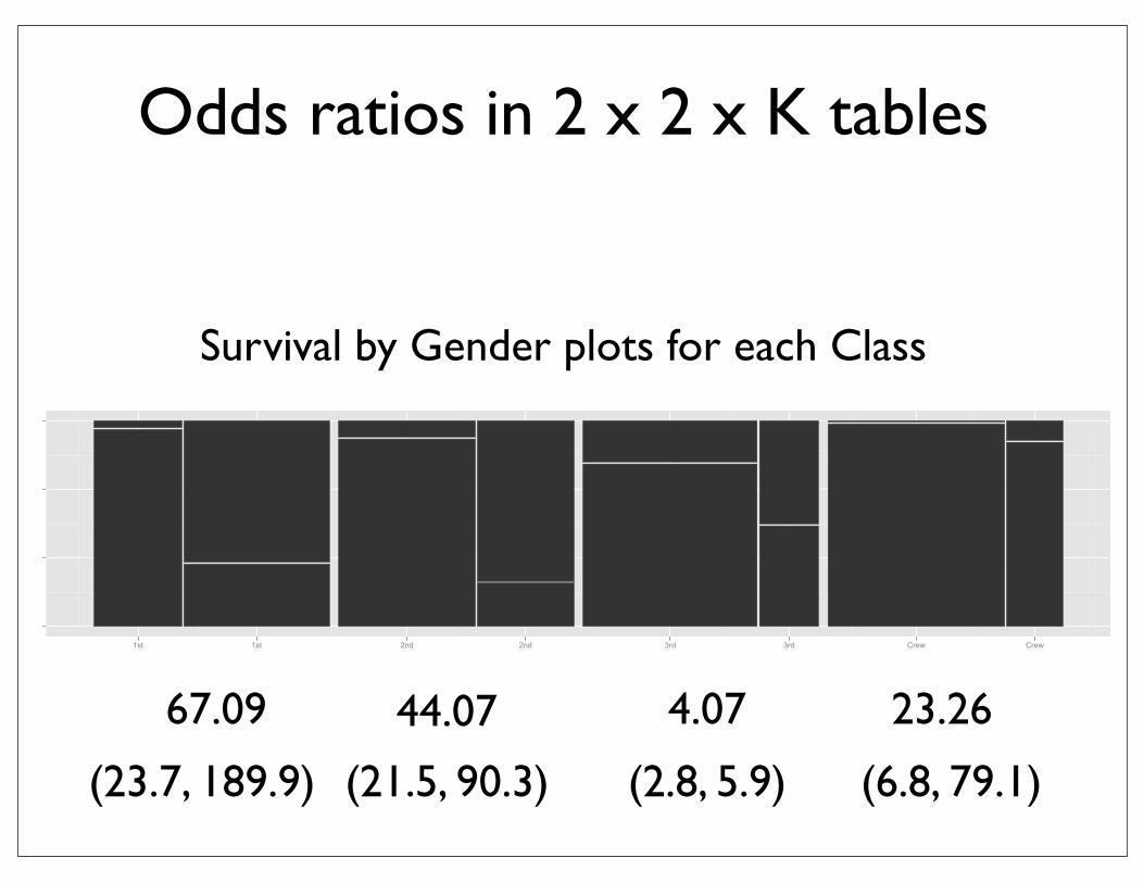
Survival by Gender plots for each Class

Odds ratios in 2 x 2 x K tables

1st 1st 2nd 2nd 3rd 3rd Crew Crew

67.09 44.07 4.07 23.26

(6.8, 79.1)(2.8, 5.9) (21.5, 90.3) (23.7, 189.9)

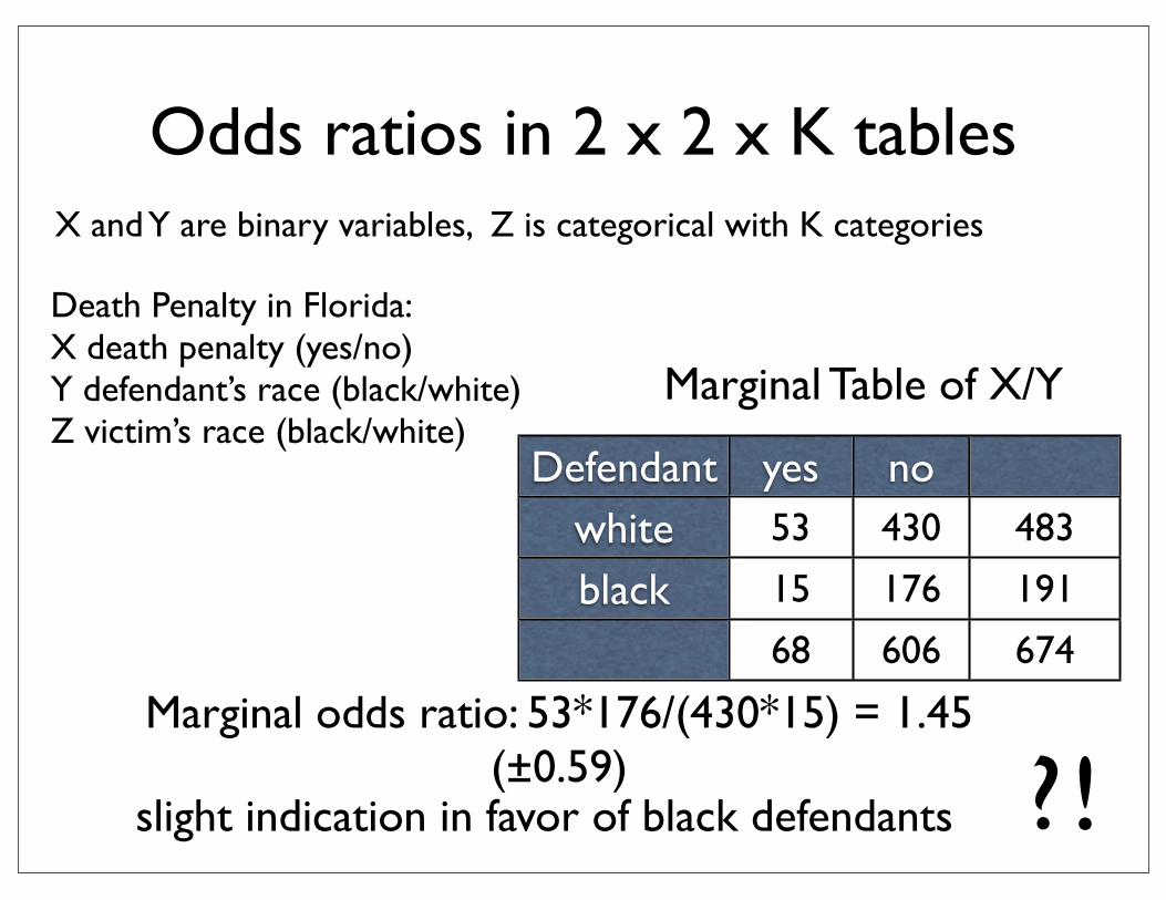
X and Y are binary variables, Z is categorical with K categories

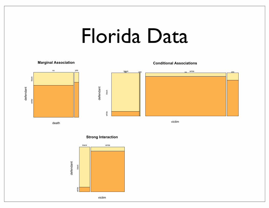
Death Penalty in Florida:X death penalty (yes/no)Y defendant’s race (black/white)Z victim’s race (black/white)

Defendant yes nowhiteblack

53 430 483

15 176 191

68 606 674

Marginal Table of X/Y

Marginal odds ratio: 53*176/(430*15) = 1.45 (±0.59)

slight indication in favor of black defendants


?!

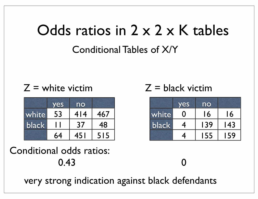
yes nowhiteblack

53 414 46711 37 4864 451 515

Conditional Tables of X/Y

Conditional odds ratios:0.43 0

Z = white victim

yes nowhiteblack

0 16 164 139 1434 155 159

Z = black victim

very strong indication against black defendants


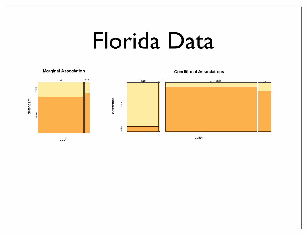
Conditional Associations

victim

defendant

black whiteno yes

black

white

no yes

Marginal Association

death

defendant

no yes

black

white

Florida Data

• Simpson’s paradox: marginal association between X and Y is opposite to conditional associations between X and Y for each level of Z

• due to: very strong marginal association between X and Z or Y and Z

Simpson’s paradox

Conditional Associations

victim

defendant

black whiteno yes

black

white

no yes

Marginal Association

death

defendant

no yes

black

white

Strong Interaction

victim

defendant

black white

black

white

Florida Data

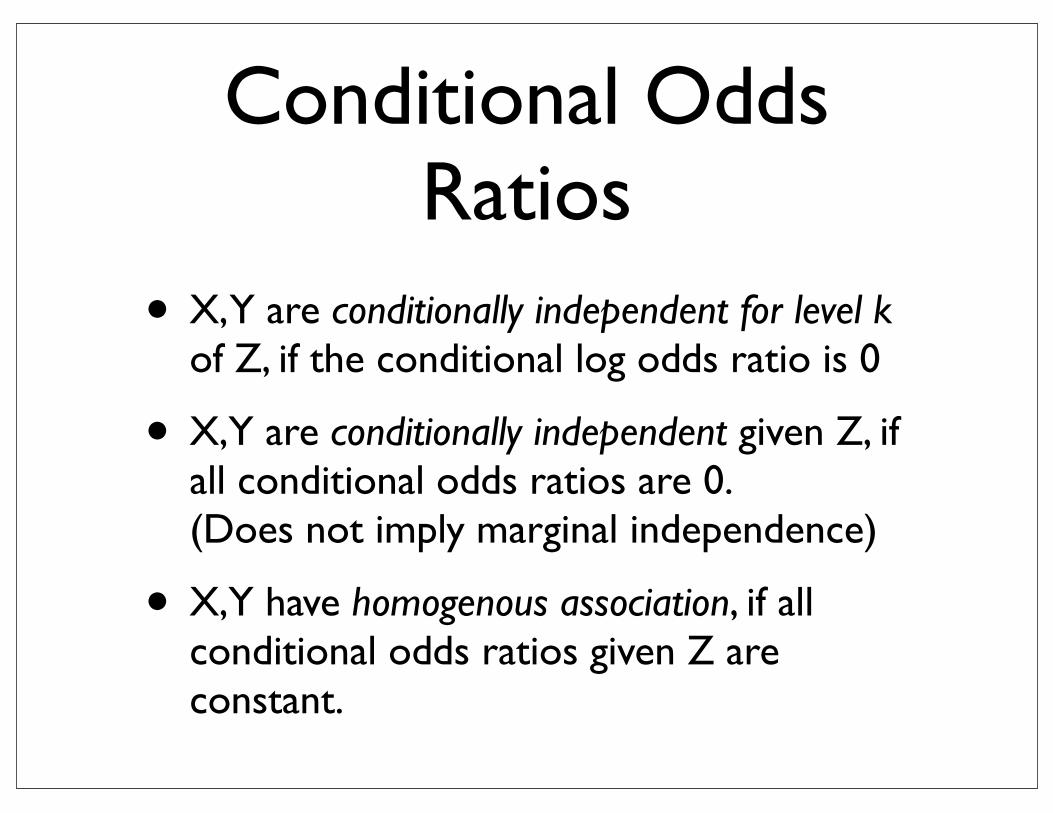
Conditional Odds Ratios

• X, Y are conditionally independent for level k of Z, if the conditional log odds ratio is 0

• X,Y are conditionally independent given Z, if all conditional odds ratios are 0.(Does not imply marginal independence)

• X,Y have homogenous association, if all conditional odds ratios given Z are constant.

Testing Independence

• Odds ratio of 1 indicates independence, confidence interval helps to determine deviation from independence, but CI is approximation.

• Alternative solution: table tests

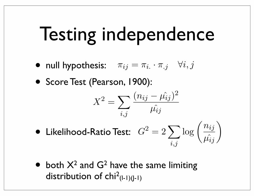
Testing independence

• null hypothesis:

• Score Test (Pearson, 1900):

• Likelihood-Ratio Test:

• both X2 and G2 have the same limiting distribution of chi2(I-1)(J-1)

πij = πi. · π.j ∀i, j


then Odds Ratio θ:

log θ = logad

bc= log

1− b

b+ log

d

1− d

Taylor≈ 4(d− b)

p̃ =y + 2

n + 4

p̃ ± zα/2

�1

np̃(1− p̃)


= ±zα/2

p +

z2α/2

2n± zα/2

��

p(1− p) +

z2α/2

4n

�/n

�

1 +

z2α/2

n

�−1

p =Y

n

|p− π|�1np(1− p)

.∼ N(0, 1)

nπ ≥ 5, n(1− π) ≥ 5

λ ·��

β2+

�α2

�

{α0m, αm : m = 1, ...,M} M(p + 1)

{β0k, βk : k = 1, ...,K} K(M + 1)

gk(T ) =eTk

�K�=1 eT�

σ(ν) =1

1 + e−ν

1

X2=

�

i,j

(nij − µ̂ij)2

µ̂ij



then Odds Ratio θ:

log θ = logad

bc= log

1− b

b+ log

d

1− d

Taylor≈ 4(d− b)

p̃ =y + 2

n + 4

p̃ ± zα/2

�1

np̃(1− p̃)


= ±zα/2

p +

z2α/2

2n± zα/2

��

p(1− p) +

z2α/2

4n

�/n

�

1 +

z2α/2

n

�−1

p =Y

n

|p− π|�1np(1− p)

.∼ N(0, 1)

nπ ≥ 5, n(1− π) ≥ 5

λ ·��

β2+

�α2

�

{α0m, αm : m = 1, ...,M} M(p + 1)

{β0k, βk : k = 1, ...,K} K(M + 1)

gk(T ) =eTk

�K�=1 eT�

1

G2= 2

�

i,j

log

�nij

µ̂ij

�

X2=

�

i,j

(nij − µ̂ij)2

µ̂ij



then Odds Ratio θ:

log θ = logad

bc= log

1− b

b+ log

d

1− d

Taylor≈ 4(d− b)

p̃ =y + 2

n + 4

p̃ ± zα/2

�1

np̃(1− p̃)


= ±zα/2

p +

z2α/2

2n± zα/2

��

p(1− p) +

z2α/2

4n

�/n

�

1 +

z2α/2

n

�−1

p =Y

n

|p− π|�1np(1− p)

.∼ N(0, 1)

nπ ≥ 5, n(1− π) ≥ 5

λ ·��

β2+

�α2

�

{α0m, αm : m = 1, ...,M} M(p + 1)

{β0k, βk : k = 1, ...,K} K(M + 1)

1

Example: Cholesterol/Heart Disease

• 1329 patients of same age/sex

present absent

Cholesterol ≤ 220

> 220

y11= 20 y12= 553

y21= 72 y22= 684

mg/l

Coronary Disease

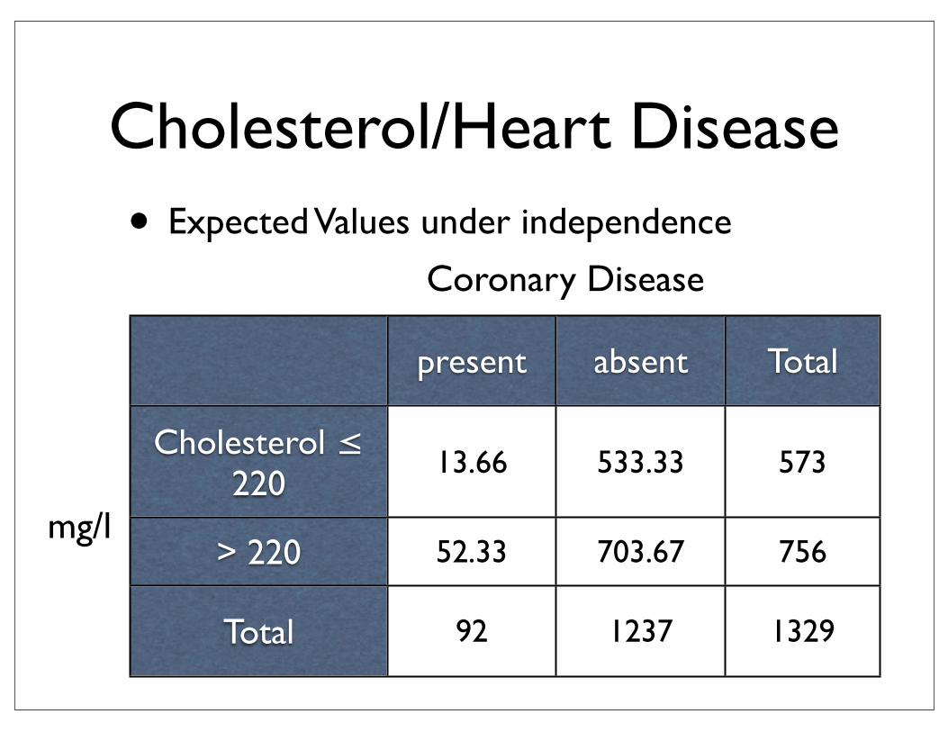
Cholesterol/Heart Disease• Expected Values under independence

present absent Total

Cholesterol ≤ 220

> 220

Total

13.66 533.33 573

52.33 703.67 756

92 1237 1329

mg/l

Coronary Disease

Cholesterol/Heart Disease

• loglikelihood ratio test G2 = 19.8

• Pearson score test X2 = 18.4

• with df = (2-1)*(2-1) = 1independence seems to be violated

Extensions to I x J Contingency Tables

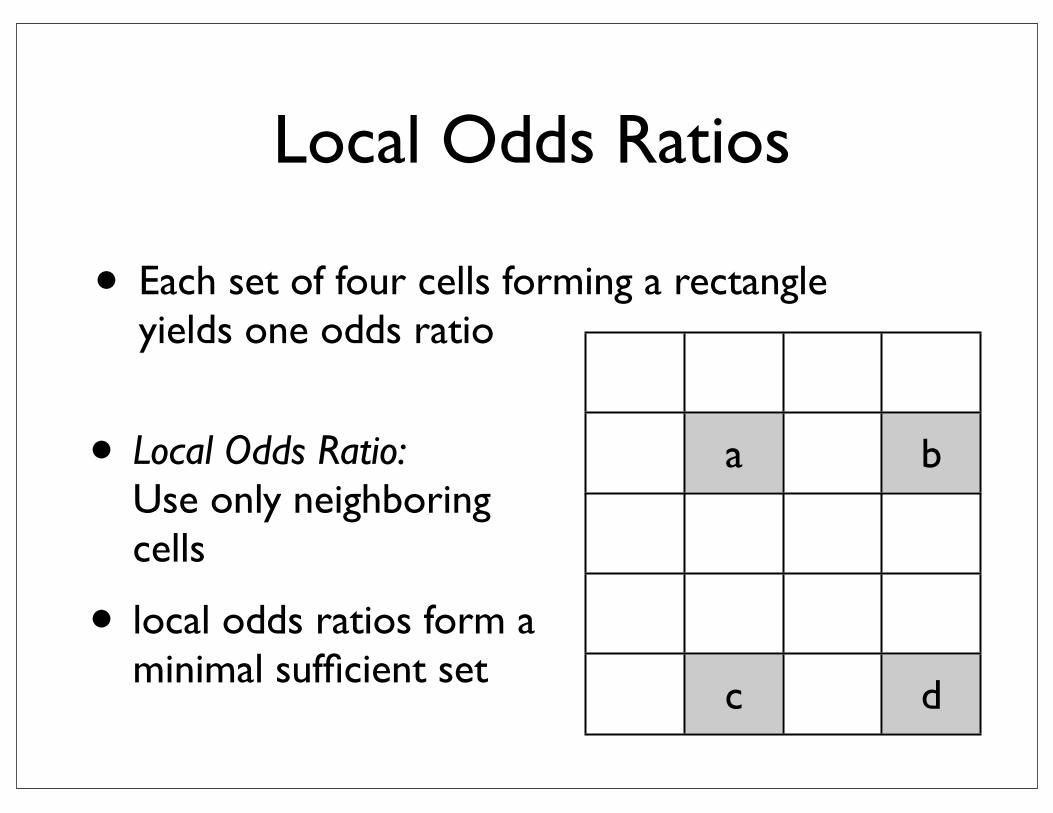
• Each set of four cells forming a rectangle yields one odds ratio

a b

c d

• Local Odds Ratio:Use only neighboring cells

• local odds ratios form a minimal sufficient set

Local Odds Ratios

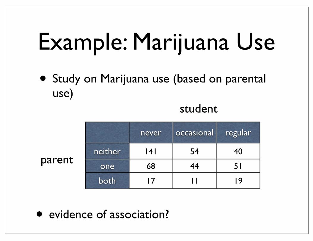
• Study on Marijuana use (based on parental use)

never occasional regular

neither

one

both

141 54 40

68 44 51

17 11 19

student

parent

• evidence of association?

Example: Marijuana Use

neither one both

• Student by Parent Use

student

parent• positive association?

Example: Marijuana Use

prodplot(mj, count~student+parent, c("vspine","hspine"), subset=level==2)

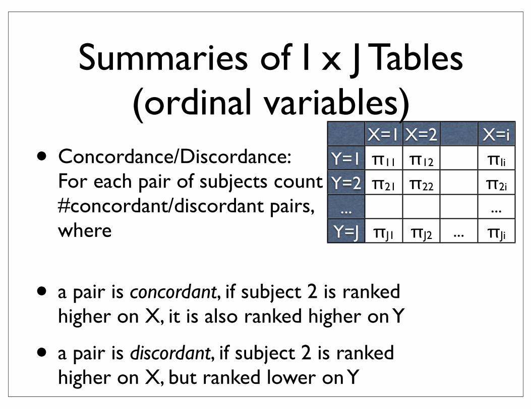
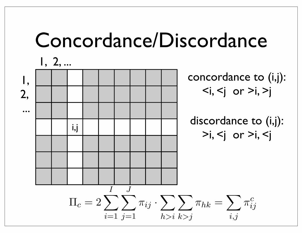
• Concordance/Discordance:For each pair of subjects count #concordant/discordant pairs, where

• a pair is concordant, if subject 2 is ranked higher on X, it is also ranked higher on Y

• a pair is discordant, if subject 2 is ranked higher on X, but ranked lower on Y

X=1 X=2 X=iY=1Y=2...

Y=J

π11 π12 πIi

π21 π22 π2i

...

πJ1 πJ2 ... πJi

Summaries of I x J Tables(ordinal variables)

i,ji,j

concordance to (i,j):<i, <j or >i, >j

i,jdiscordance to (i,j):

>i, <j or >i, <j

Concordance/Discordancegk(T ) =eTk

�K�=1 eT�

σ(ν) =1

1 + e−ν

Zm = σ(α0m + α�mX) m = 1, ...,M

Tk = β0k + β�kZ k = 1, ...,K

fk(X) = gk(T ) k = 1, ...,K

Πc = 2I�

i=1

J�

j=1

πij ·�

h>i

�

k>j

πhk =�

i,j

πcij

σ2(γ̂)∞ =16

n(ΠC + ΠD)4

I�

i=1

J�

j=1

πij

�ΠCπd

ij −ΠDπcij

�2

γ =ΠC −ΠD

ΠC + ΠD

θ :=π00 π11

π10 π01

π : (1− π)

πj|i=0 − πj|i=1 =: π1 − π2,

r :=πj=1|i=0

πj=1|i=1

χ21,0.05 = 3.84, χ2

1,0.01 = 6.634897

πij = πi+ · π+j


π11

π11 + π12=

π21

π21 + π22

2

1, 2, ...

1, 2, ...

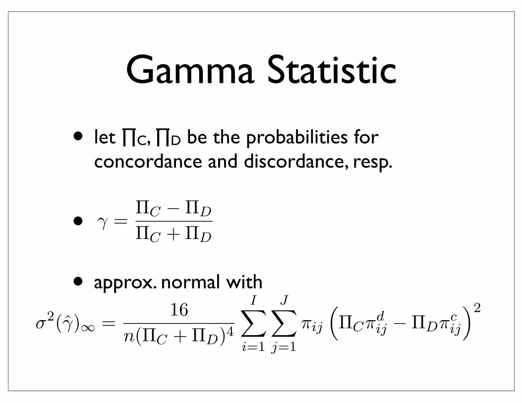
• let ∏C, ∏D be the probabilities for concordance and discordance, resp.

•

• approx. normal with

Gamma Statistic

σ2(γ̂)∞ =16

n(ΠC + ΠD)4

I�

i=1

J�

j=1

πij

�ΠCπd

ij −ΠDπcij

�2

γ =ΠC −ΠD

ΠC + ΠD

θ :=π00 π11

π10 π01

π : (1− π)

πj|i=0 − πj|i=1 =: π1 − π2,

r :=πj=1|i=0

πj=1|i=1

χ21,0.05 = 3.84, χ2

1,0.01 = 6.634897

πij = πi+ · π+j


π11

π11 + π12=

π21

π21 + π22



X\Y y1 y2 ... yJ

x1 n11 n12 ... n1J n1.

x2 n21 n22 ... n2J n2....

...... . . . ...


n.1 n.2 ... n.J n

2

σ2(γ̂)∞ =16

n(ΠC + ΠD)4

I�

i=1

J�

j=1

πij

�ΠCπd

ij −ΠDπcij

�2

γ =ΠC −ΠD

ΠC + ΠD

θ :=π00 π11

π10 π01

π : (1− π)

πj|i=0 − πj|i=1 =: π1 − π2,

r :=πj=1|i=0

πj=1|i=1

χ21,0.05 = 3.84, χ2

1,0.01 = 6.634897

πij = πi+ · π+j


π11

π11 + π12=

π21

π21 + π22



X\Y y1 y2 ... yJ

x1 n11 n12 ... n1J n1.

x2 n21 n22 ... n2J n2....

...... . . . ...


n.1 n.2 ... n.J n

2

statistics of contingency tables - hofroe.net · contingency tables stat 557 heike hofmann. outline...

Documents