statistics of co-channel interference in a field of...
TRANSCRIPT

1
Statistics of Co-Channel Interference in a Field ofPoisson and Poisson-Poisson Clustered Interferers
Kapil Gulati, Student Member, IEEE, Brian L. Evans, Fellow, IEEE, Jeffrey G. Andrews, Senior Member, IEEE,and Keith R. Tinsley, Senior Member, IEEE
Abstract—With increasing spatial reuse of radio spectrum, co-channel interference is becoming a dominant noise source andmay severely degrade the communication performance of wirelesstransceivers. In this paper, we consider the problem of statistical-physical modeling of co-channel interference from an annularfield of Poisson or Poisson-Poisson cluster distributed interferers.Poisson and Poisson-Poisson cluster processes are commonlyused to model interferer distributions in large wireless networkswithout and with interferer clustering, respectively. Further, byconsidering the interferers distributed over a parametric annularregion, we derive interference statistics for finite- and infinite-area interference region with and without a guard zone aroundthe receiver. Statistical modeling of interference is a useful toolto analyze outage probabilities in wireless networks and designinterference-aware transceivers. Our contributions include (1)developing a unified framework for deriving interference modelsfor various wireless network environments, (2) demonstratingthe applicability of the symmetric alpha stable and Gaussianmixture (with Middleton Class A as a particular form) distri-butions in modeling co-channel interference, and (3) derivinganalytical conditions on the system model parameters for whichthese distributions accurately model the statistical propertiesof the interference. Applications include co-channel interferencemodeling for various wireless networks, including wireless ad hoc,cellular, local area, and femtocell networks.
Index Terms—Co-channel interference, Poisson processes, im-pulsive noise, probability, stochastic approximation.
I. INTRODUCTION
Current and future wireless communication systems requirehigher spectral usage due to increasing demand in user datarates. One of the principal techniques for efficient spectralusage is to implement a dense spatial reuse of the availableradio spectrum. This causes severe co-channel interference,which limits the communication system performance. Knowl-edge of interference statistics is integral to analyzing per-formance of wireless networks, including outage probabilityand throughput, and can also be used to design transceiverswith improved communication performance [1]–[6]. We havereleased a freely distributed software toolbox for statisticalmodeling and mitigation of radio frequency interference [7].
Copyright (c) 2010 IEEE. Personal use of this material is permitted.However, permission to use this material for any other purposes must beobtained from the IEEE by sending a request to [email protected].
K. Gulati, B. L. Evans, and J. G. Andrews are with the Department ofElectrical and Computer Engineering, The University of Texas at Austin, TX,78712 USA e-mail: gulati, bevans, [email protected].
K. R. Tinsley is with Intel Corporation, Santa Clara, CA 95054 USA e-mail:[email protected].
This research was supported by Intel Corporation.Manuscript submitted November 29, 2009; revised April 3, 2010; accepted
August 12, 2010.
A. Motivation and Prior Work
Co-channel interference statistics in wireless networks areaffected by the following key factors: (i) the spatial distributionof interferers, (ii) the spatial region over which the interferersare distributed, and (iii) propagation characteristics includingthe power pathloss exponent and fading. Regarding (i), thedistribution of active interferers in large random wirelessnetworks is generally assumed to be a homogeneous spatialPoisson point process [6], [8]–[11]. While this assumption maybe valid for certain wireless networks (e.g. wireless sensor andad hoc networks), it may be common for interfering users tocluster in space due to geographical factors (e.g. gatheringplaces or femtocell networks [12], [13]), or medium accesscontrol (MAC) layer protocols [6], [14]. Regarding (ii), thespatial region containing the interferers is commonly assumedto be an infinite plane [8]–[11]. Many wireless networks,however, employ contention-based MAC protocols (e.g. car-rier sense multiple access and multiple access with collisionavoidance) or other local coordination techniques to limitthe interference, thereby creating a guard zone around thereceiver (e.g. in wireless ad hoc networks [15] and in denseWi-Fi networks [6], [16]). Guard zones around the receivercan also occur due to scheduling-based MAC protocols, suchas in cellular networks in which the users in the same cellsite are orthogonal to each other and all interfering usersare outside the cell site in which the receiver is located.Further, receivers in many wireless networks may experienceinterference from finite-area regions (e.g. interference from acell cite in cellular networks with reuse factor greater than one)[17]. This motivates characterizing the interference statistics inPoisson and Poisson-Poisson clustered interferers distributedover a parametric annular region. For each of the interfererdistributions, the finite- and infinite- area with and withouta guard zone around the receiver can then be studied asparticular cases of the parametric annular interference region.
The statistical techniques used in modeling interferenceinclude empirical methods and statistical-physical methods.Empirical approaches fit a mathematical model to measuredreceived signals, without regard to the physical generationmechanisms behind the interference. Statistical-physical mod-els, on the other hand, model interference based on the phys-ical principles that govern the generation and propagation ofthe interference-causing emissions. Statistical-physical modelsare thus more widely applicable than empirical models [18],[19].
Statistical-physical modeling of co-channel interference in
2
random Poisson interference fields has been extensively stud-ied in literature [17], [20]–[24]. In [20], it was shown thatinterference from a homogeneous Poisson field of interferersdistributed over the entire plane can be modeled using thesymmetric alpha stable distribution [25]. This result was laterextended to include channel randomness [21] and second-orderstatistics capturing the temporal dependence [22]. Recently,the authors in [17] investigated extensions for a finite-areafield and derived the interference moments. Closed formapproximations to the interference distribution, however, werenot investigated. In our prior work [23], [24], we presented aunified framework from which we derived the co-channel in-terference statistics in a Poisson field of interferers distributedon a parametric circular annular region. In this paper, weextend the work in [24] for wider range of interferer topologiesand Poisson-Poisson cluster field of interferers.
Other key statistical-physical models for co-channel inter-ference in random Poisson interference fields include Middle-ton Class A, B, and C models [19]. Middleton models areuseful because they characterize a wider range of physicalconditions, including narrowband and broadband interferenceemissions, transients at the receiver, and background thermalnoise [18], [19]. Middleton models, however, have not beenwidely used to characterize co-channel interference in wirelessnetwork environments.
Statistical-physical modeling of co-channel interference inrandom Poisson clustered interference fields was recentlystudied in [26]. The focus of the work was to characterizethe network performance (outage probability and transmissioncapacity) and the interferer clusters were assumed to bedistributed over the entire plane. Closed form interferencestatistics, however, were not derived.
The problem considered in this paper is also closely relatedto the problem of deriving the amplitude distribution of shotnoise processes [27]. Co-channel interference in a planarnetwork of nodes distributed according to any point processcan be modeled as a generalized shot noise process [27], [28].The shot noise process is studied in detail in [27] and existenceof generalized shot noise process for any point process wasshown in [28]. Properties of the shot noise processes, such ascharacteristic function for power-law shot noise process [29],are commonly used to evaluate bounds on outage probabilitiesin wireless networks [13], [30]. To the best of our knowledge,closed form expression of the amplitude distribution for shotnoise process are not known for the interferer topologiesconsidered in this paper.
B. Contribution, Organization, and Notation
In this paper, we derive the interference statistics froma field of Poisson and Poisson-Poisson clustered distributedinterferers. Further, for each of the interferer distributions,we derive the statistics for interferers or interferer clustersdistributed over (i) the entire plane, (ii) finite-area annularregion, and (iii) infinite-area annular region with a guard zonearound the desired receiver. One of the key contributions ofthis paper is to develop a unified framework to derive theco-channel interference statistics in different wireless network
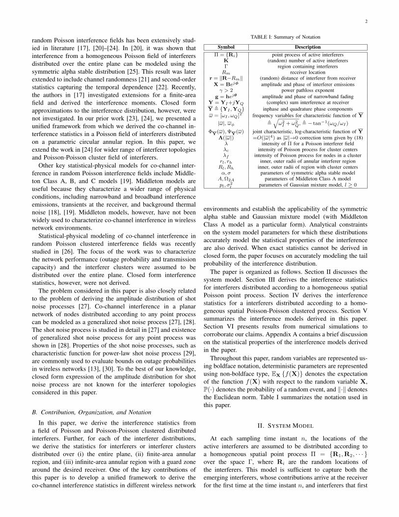
TABLE I: Summary of Notation
Symbol DescriptionΠ = Ri point process of active interferers
K (random) number of active interferersΓ region containing interferersRm receiver location
r = ‖R−Rm‖ (random) distance of interferer from receiverX = Bejφ amplitude and phase of interferer emissionsγ > 2 power pathloss exponent
g = hejθ amplitude and phase of narrowband fadingY = YI+jYQ (complex) sum interference at receiverY , YI ,YQ inphase and quadrature phase componentsω = [ωI , ωQ]T frequency variables for characteristic function of Y
|ω|, ωφ ,√ω2I + ω2
Q, , − tan−1(ωQ/ωI)
ΦY(ω),ΨY(ω) joint characteristic, log-characteristic function of YΛ(|ω|) =O(|ω|4) as |ω|→0 correction term given by (18)λ intensity of Π for a Poisson interferer fieldλc intensity of Poisson process for cluster centersλf intensity of Poisson process for nodes in a clusterrl, rh inner, outer radii of annular interferer regionRl, Rh inner, outer radii of region with cluster centersα, σ parameters of symmetric alpha stable model
A,Ω2A parameters of Middleton Class A modelpl, σ
2l parameters of Gaussian mixture model, l ≥ 0
environments and establish the applicability of the symmetricalpha stable and Gaussian mixture model (with MiddletonClass A model as a particular form). Analytical constraintson the system model parameters for which these distributionsaccurately model the statistical properties of the interferenceare also derived. When exact statistics cannot be derived inclosed form, the paper focuses on accurately modeling the tailprobability of the interference distribution.
The paper is organized as follows. Section II discusses thesystem model. Section III derives the interference statisticsfor interferers distributed according to a homogeneous spatialPoisson point process. Section IV derives the interferencestatistics for a interferers distributed according to a homo-geneous spatial Poisson-Poisson clustered process. Section Vsummarizes the interference models derived in this paper.Section VI presents results from numerical simulations tocorroborate our claims. Appendix A contains a brief discussionon the statistical properties of the interference models derivedin the paper.
Throughout this paper, random variables are represented us-ing boldface notation, deterministic parameters are representedusing non-boldface type, EX f(X) denotes the expectationof the function f(X) with respect to the random variable X,P(·) denotes the probability of a random event, and ‖·‖ denotesthe Euclidean norm. Table I summarizes the notation used inthis paper.
II. SYSTEM MODEL
At each sampling time instant n, the locations of theactive interferers are assumed to be distributed according toa homogeneous spatial point process Π = R1,R2, · · · over the space Γ, where Ri are the random locations ofthe interferers. This model is sufficient to capture both theemerging interferers, whose contributions arrive at the receiverfor the first time at the time instant n, and interferers that first

3
emerged at some prior sampling time instant m < n but arestill active till the sample time n [22].
The baseband model for the sum interference Y at any timeinstant can then be represented as
Y =
K∑i=1
r− γ2i giXi (1)
where K is the random number of active interferers at thattime instant, i is the interferer index, ri = ‖Ri − Rm‖ arethe random distances of active interferers from the receiver,γ is the power pathloss exponent, gi is the independent andidentically distributed (i.i.d.) random fast fading experiencedby each interferer emission, and Xi are the random interfereremissions.
We assume that all potential interferers have i.i.d. symmetricnarrowband emissions of the form [18]
Xi = Biejφi = Bi cos(φi) + jBi sin(φi) (2)
where Bi is the i.i.d. envelope, and φi is the i.i.d. randomphase of the emissions. Further, we assume that the emergingtimes of the interferers are uniformly distributed between thesampling times at the receiver. Thus the phase φi of the emis-sions at the sampling instants can be assumed to be uniformlydistributed on [0, 2π]. The assumption of i.i.d. emissions isvalid for wireless communication networks without powercontrol and may not be true for modeling interference fromdiverse types of interferers with unequal transmit power (e.g.base stations and mobile users).
The fast fading experienced by the interferer emissions isalso assumed to be narrowband of the form
gi = hiejθi (3)
where hi is the random amplitude scaling and θi is the randomphase variation due to fading. The in-phase and quadrature-phase components of the emissions are assumed to experienceuncorrelated fading and thus θi is uniformly distributed on[0, 2π]. The sum interference can be expressed as
Y =
K∑i=1
r− γ2i hiBi cos(φi+θi) + j
K∑i=1
r− γ2i hiBi sin(φi+θi)
(4)
III. CO-CHANNEL INTERFERENCE IN A POISSON FIELD OFINTERFERERS
Consider a scenario, as shown in Fig. 1, in which the spatialpoint process Π in (1) is a homogeneous spatial Poisson pointprocess with intensity λ and the interferers are distributedover the space Γ(rl, rh). The parametric interference spaceis defined as
Γ(rl, rh) =x ∈ R2 : rl ≤ ‖x‖ ≤ rh
. (5)
From (4), the joint characteristic function of the in-phase andquadrature-phase components of the sum interference Y =YI + jYQ can be expressed as
ΦYI ,YQ(ωI , ωQ)
= EYI ,YQ
ejωIYI+jωQYQ
= Eej∑Ki=1 r
− γ2
i hiBi(ωI cos(φi+θi)+ωQ sin(φi+θi))
= E
ej|ω|
∑Ki=1 r
− γ2
i hiBi cos(φi+θi+ωφ)
(6)
=
∞∑k=0
Eej|ω|
∑ki=1 r
− γ2
i hiBi cos(φi+θi+ωφ)∣∣k in Γ(rl, rh)
× P (k in Γ(rl, rh)) (7)
where ω = [ωI , ωQ]T , |ω| =√ω2I + ω2
Q, and ωφ =
− tan−1(ωQωI
). The expectation in (7) is with respect to the
set of random variables ri,hi,Bi,φi,θi.Conditioned on the number of interferers present in the
space Γ(rl, rh), the interferer locations are mutually inde-pendent and uniformly distributed across this space [25].Henceforth, we remove the conditioning on the number of in-terferers from the expectation by noting that the interferers areuniformly distributed over Γ(rl, rh). Further, in the absence ofpower control, the interferer emissions can be assumed to bei.i.d.. The characteristic function can then be expressed as
ΦY(ω) =
∞∑k=0
[Eej|ω|r
− γ2 hB cos(φ+θ+ωφ)
]k×
[λπ(r2h − r2
l
)]ke−λπ(r2
h−r2l )
k!(8)
= eλπ(r2
h−r2l )
(Eej|ω|r
− γ2 hB cos(φ+θ+ωφ)
−1
)(9)
where Y is the set YI ,YQ. By taking the logarithm ofΦY(ω), the log-characteristic function is
ψY(ω) , log ΦY(ω)
= λπ(r2h − r2
l
) (Eej|ω|r
− γ2 hB cos(φ+θ+ωφ)
− 1).
(10)
By using the identity
eja cos(φ) =
∞∑k=0
jkεkJk(a) cos(kφ) (11)
where ε0 = 1, εk = 2 for k ≥ 1, and Jk(·) denotes theBessel function of order k, the log-characteristic function canbe expressed as
ψY(ω) = λπ(r2h − r2
l
)(E ∞∑k=0
jkεkJk
(|ω|r−
γ2 hB
)×
cos (k(φ + θ + ωφ))− 1
). (12)
Since φ and θ are assumed to be uniformly distributed on[0, 2π], Eφ,θ cos (k(φ + θ + ωφ)) = 0 for k ≥ 1, and (12)reduces to
ψY(ω) = λπ(r2h − r2
l
) (Er,h,B
J0
(|ω|r−
γ2 hB
)− 1).
(13)The log-characteristic function derived in (13) holds in generalfor narrowband interferers distributed over the parametricspace Γ(rl, rh), governed by the parameters rh and rl and
4
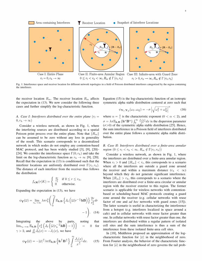
Fig. 1: Interference space and receiver location for different network topologies in a field of Poisson distributed interferers categorized by the region containingthe interferers.
the receiver location Rm. The receiver location Rm affectsthe expectation in (13). We now consider the following threecases and further simplify the log-characteristic function.
A. Case I: Interferers distributed over the entire plane (rl =0, rh →∞)
Consider a wireless network, as shown in Fig. 1, wherethe interfering sources are distributed according to a spatialPoisson point process over the entire plane. Note that ‖Rm‖can be assumed to be zero without any loss in generalityof the result. This scenario corresponds to a decentralizednetwork in which nodes do not employ any contention-basedMAC protocol, and has been widely studied [3], [9], [20]–[24]. We consider the interference space Γ(0, rh) and take thelimit on the log-characteristic function as rh → ∞ [9], [20].Recall that the expectation in (13) is conditioned such that theinterferer locations are uniformly distributed over Γ(rl, rh).The distance of each interferer from the receiver thus followsthe distribution
fr|K(r|K) =
2rr2h
if 0 ≤ r ≤ rh,0 otherwise.
Expanding the expectation in (13), we have
ψY(ω) = limrh→∞
λπr2h
( rh∫0
Eh,B
J0
(|ω|r−
γ2 hB
) 2r
r2h
dr
− 1
). (14)
Integrating the above by parts, noting thatlimrh→∞ Eh,B
r2h
(J0
(|ω|r−
γ2
h hB)− 1)
= 0 for
γ > 2, and ddxJ0(x) = −J1(x), we have
ψY(ω) = −|ω|4γ λπEh,B
h
4γ B
4γ
∞∫0
J1(x)
x4γ
dx. (15)
Equation (15) is the log-characteristic function of an isotropicsymmetric alpha stable distribution centered at zero such that
ψYI ,YQ(ωI , ωQ) = −σ
∣∣∣√ω2I + ω2
Q
∣∣∣α (16)
where α = 4γ is the characteristic exponent (0 < α < 2), and
σ = λπEh,B hαBα∫∞
0J1(x)xα dx is the dispersion parameter
(σ>0) of the symmetric alpha stable distribution [25]. Hence,the sum interference in a Poisson field of interferers distributedover the entire plane follows a symmetric alpha stable distri-bution.
B. Case II: Interferers distributed over a finite-area annularregion (0 ≤ rl < rh <∞, Rm /∈ Γ(rl, rh))
Consider a wireless network, as shown in Fig. 1, wherethe interferers are distributed over a finite-area annular region.When rl > 0 and ‖Rm‖ < rl, this corresponds to a scenariowhere all the interferers are outside a guard zone aroundthe receiver and within a maximum distance (rh < ∞)beyond which they do not generate significant interference.When ‖Rm‖ > rh, this corresponds to a scenario where theinterferers are distributed over a finite-area circular or annularregion with the receiver exterior to this region. The formerscenario is applicable for wireless networks with contention-based or scheduling-based MAC protocols creating a guardzone around the receiver (e.g. cellular networks with reusefactor of one and ad hoc networks with guard zones [15]).The latter scenario is useful in characterizing the interferencefrom a hotspot (e.g. interferers localized in space around acafe) and in cellular networks with reuse factor greater thanone. In cellular networks with reuse factor greater than one, theinterferers are distributed within a regular pattern of isolatedcell sites and the sum interference is thus a sum of theinterference from these isolated finite-area cell sites.
In [18], Middleton proposed an approximation of the log-characteristic function for |ω| in the neighborhood of zero.From Fourier analysis, the behavior of the characteristic func-tion for |ω| in the neighborhood of zero governs the tail prob-

5
ability of the random envelope. The proposed approximationis based on the following identity [18]:
Er,h,B
J0
(|ω|r−
γ2 hB
)= e−
|ω|2Er,h,Br−γh2B24 ×
(1 + Λ(|ω|)) (17)
where Λ(|ω|)) indicates a correction term with the lowestexponent in |ω| of four and is given by
Λ(|ω|)) =
∞∑k=2
(EZ Z)k |ω|2k
22kk!EZ
1F1
(−k; 1;
Z
EZ Z
)(18)
where the random variable Z = r−γh2B2, and 1F1 (a; b;x) isthe confluent hypergeometric function of the first kind, suchthat Λ(|ω|) = O(|ω|4) as |ω| → 0.
Using this identity, and approximating Λ (|ω|) << 1 for |ω|in the neighborhood of zero, the log-characteristic function in(13) can be expressed as
ψY(ω) ≈ λπ(r2h − r2
l
)(e−|ω|2Er,h,Br−γh2B2
4 − 1
). (19)
Equation (19) is the log-characteristic function of a MiddletonClass A distribution such that
ψYI ,YQ(ωI , ωQ) = A
(e−
(ω2I+ω2
Q)Ω2A
2A − 1
)(20)
where A = λπ(r2h − r2
l
)is the overlap index that indi-
cates the amount of impulsiveness of the interference, and
Ω2A =A×Er,h,Br−γh2B2
2 is the mean intensity of theinterference [19]. Hence, the co-channel interference from afield of Poisson distributed interferers over the finite-area spaceΓ(rl, rh) with Rm /∈ Γ(rl, rh) follows the Middleton Class Adistribution. It should be emphasized that the correspondenceto the Middleton Class A distribution is particularly valid formodeling the tail probabilities.
The approximation in (17) and the subsequent interferencemodel in (20) is valid for Rm /∈ Γ(rl, rh), since Ω2A → ∞as ‖Rm‖ → rl or as ‖Rm‖ → rh. This is unlike Case I inSection III-A where the interference was modeled for rl = 0.This is the key difference between the symmetric alpha stableand Middleton Class A models for interference.
Next, we quantify the range of the system model parametersover which the Middleton Class A model provides an accurateapproximation to the co-channel interference in this scenario.From (17), a first-order measure of the accuracy of theapproximation can be expressed by comparing the coefficient
of |ω|4 term in e−|ω|2Er,h,Br−γh2B2
4 against the coefficientof |ω|4 in the correction term Λ(|ω|). Using the fact that
1F1 (−2; 1;x) =1
2(x2 − 4x+ 2), (21)
the coefficient of |ω|4 in the correction term (i.e., c4) can beexpressed as
c4 =EZ
Z2− 2 [EZ Z]2
128. (22)
Thus, the Middleton Class A model provides a good approx-imation when the system parameters, such as rh, rl, Rm, andγ, satisfy ∣∣∣∣∣EZ
Z2− 2 [EZ Z]2
128
∣∣∣∣∣ << [EZ Z]2
32(23)
⇒
∣∣∣∣∣ Er,h,B
r−2γh4B4
4× [Er,h,B r−γh2B2]2
− 1
2
∣∣∣∣∣ << 1. (24)
To provide some intuition about the above result, for a non-random h and B, the condition is satisfied when ‖Rm‖ << rland rl
rhis greater than a fraction that depends on γ and Rm,
or when ‖Rm‖ >> rh. The conditions ‖Rm‖ << rl and‖Rm‖ >> rh ensure that the interferers are not close to thereceiver and a lower bound on rl
rhensures that rh is not very
large compared to rl when ‖Rm‖ < rl.
C. Case III: Interferers distributed over infinite-area annularregion with guard zone (rl > 0, rh →∞, and ‖Rm‖ < rl)
Consider a wireless network, as shown in Fig. 1, wherethe interfering sources are distributed according to a spatialPoisson point process on the entire plane, except within aguard zone around the receiver. The applicability of Case IIfor guard zone scenarios was limited to finite-area fields anddoes provide a good approximation for a wide range of systemparameters. In this subsection, we allow the interference regionto have infinite area and is thereby more applicable to largerandom wireless networks with guard zones [15]. We considerthe interference space Γ(rl, rh) and take the limit on the log-characteristic function as rh →∞. Conditioned on the numberof interferers in Γ(rl, rh), the interferer locations are mutuallyindependent and uniformly distributed in the space Γ(rl, rh).Thus as rh → ∞, with high probability, the distance of aninterferer from receiver located at Rm can be approximatedas r = ‖R−Rm‖ ≈ ‖R‖, particularly for ‖Rm‖ << rl. Thedistance of each interferer from the receiver thus follows thedistribution
fr|K(r|K) =
2r
r2h−r
2l
if rl ≤ r ≤ rh,0 otherwise.
Expanding the expectation in (13), we have
ψY(ω)= limrh→∞
λπ(r2h−r2
l )
( rh∫rl
Eh,B
J0
(|ω|r−
γ2 hB
)×
2r
r2h − r2
l
dr − 1
). (25)
Integrating the above by parts, reordering terms, and notingthat lim
rh→∞λπr2
h
(Eh,B
J0
(|ω|r−
γ2
h hB)−1)
= 0 for γ >2, we have
ψY(ω) = −λπr2l
(Eh,B
J0
(|ω|r−
γ2
l hB)−1)−
limrh→∞
λπ
rh∫rl
∂
∂r
(Eh,B
J0
(|ω|r−
γ2 hB
))r2dr. (26)

6
Invoking the identity (17), and approximating Λ (|ω|) << 1for |ω| in the neighborhood of zero, the log-characteristicfunction can be expressed as
ψY(ω) ≈ − λπr2l
(e−|ω|2r−γ
lEh,Bh2B2
4 − 1
)−
limrh→∞
λπ
∫ rh
rl
∂
∂r
(e−|ω|2r−γEh,Bh2B2
4
)r2dr. (27)
Note that unlike (17), the approximation in (27) involves anon-random r. Using Taylor series expansion of ex, the log-characteristic function reduces to
ψY(ω) = λπr2l
[ ∞∑k=1
(−1)k|ω|2k
4kk!
(Eh2B2
)kr−γkl
2
kγ − 2
](28)
valid for γ > 2. The 2kγ−2 multiplicative factor inside
the summation prevents the log-characteristic function to beexpressed in closed form. We thus approximate the function
2kγ−2 as ηeβk for k ≥ 1. The parameters η and β are chosento minimize the weighted mean squared error (WMSE)
η, β = arg minη,β
∞∑k=1
(2
kγ − 2− ηeβk
)2
u(k) (29)
where u(k) are the weights. The weights should be chosensuch that penalty of error is large when k is small, since itaffects the coefficients of terms with lower order exponentsof |ω|. Equation (29) is an unconstrained nonlinear optimiza-tion problem and can be solved efficiently using numeri-cal techniques such as quasi-Newton methods [31]. Quasi-Newton methods have superlinear convergence and requireO(ln(| ln(ε)|)) number of iterations and O(d2 ln(| ln(ε)|)) al-gebraic computational effort, where d is the dimensionality ofthe problem and ε is the maximum permissible error tolerancein the result. Table II lists the values for η, β and theassociated WMSE for certain values of γ, using the weightsu(k) = e−k. By approximating 2
kγ−2 as ηeβk for k ≥ 1, thelog-characteristic exponent can be expressed as
ψY(ω) ≈ λπr2l η
(e−|ω|2r−γ
leβEh,Bh2B2
4 − 1
). (30)
Equation (30) is the log-characteristic function of a MiddletonClass A distribution such that
ψYI ,YQ(ωI , ωQ) = A
(e−
(ω2I+ω2
Q)Ω2A
2A − 1
)(31)
where A = λπr2l η is the overlap index that indi-
cates the impulsiveness of the interference, and Ω2A =A×r−γl eβEh,Bh2B2
2 is the mean intensity of the interference[19].
The functional form of ηeβk to approximate 2kγ−2 for
k ≥ 1 was chosen since, a) it provides a good approximationand enables the log-characteristic function to be expressed inclosed form, and b) provides two parameters η, β such thatη affects only the impulsive index A, while β affects onlythe variance σ2
m = mAΩ2A of individual components of the
Gaussian mixture form of Middleton Class A model.
TABLE II: Values for η, β and the associated weighted mean squared error(WMSE), obtained by solving (29), for different values of the power pathlossexponent (γ) and using the weighting function u(k) = e−k . Solution to (29)was obtained by using the fminunc function in MATLAB, which uses theBFGS quasi-Newton method [31].
γ η, β WMSE
2.5 22.818,−1.741 4.32× 10⁻³
3.0 7.484,−1.321 1.84× 10⁻³
3.5 4.132,−1.132 9.81× 10⁻⁴
4.0 2.781,−1.025 5.96× 10⁻⁴
4.5 2.073,−0.954 3.96× 10⁻⁴
5.0 1.645,−0.905 2.80× 10⁻⁴
Similar to Case II, a first-order measure of accuracy of theapproximation can be expressed by comparing the coefficientof |ω|4 term in the true log-characteristic function (26) againstthe the coefficient of |ω|4 term in the approximated log-characteristic function (30). The two approximations involvedare using ηeβk to approximate the function 2
kγ−2 for k ≥ 1,and approximating Λ (|ω|) << 1 for |ω| close to zero. Notethat the lowest order term affected by the former approxima-tion is the coefficient of |ω|2 term. We assume, however, thatthe approximation error is negligible due to the optimizationin (29). Using (17) and (18), the coefficient of |ω|4 term inthe true log-characteristic function (30) is
λπr−2γ+2l
(EZ2
+ 2 [E Z]2
128
)(2
2γ − 2
)where Z = h2B2. Comparing with the coefficient of |ω|4term in (30), the Middleton Class A distribution provides agood approximation to co-channel interference statistics in thisscenario when∣∣∣∣∣(
[E Z]2
64
)(2
2γ − 2−2ηe2β
)+
(EZ2
128
)(2
2γ − 2
)∣∣∣∣∣<<
∣∣∣∣∣ [E Z]232ηe2β
∣∣∣∣∣ . (32)
Note that if ηe2β = 22γ−2 , then the above condition is same as
the one obtained for Case II in (23), with the exception thatZ = h2B2 in this case. The above condition is independentof the parameter rl that governs the interference space and isvalid when the variance of h2B2 is low when compared to[Eh2B2]2. The above condition does not capture the errordue to the approximation r = ‖R−Rm‖ ≈ R, which is truewith high probability in this scenario and is particularly validfor ‖Rm‖ << rl.
IV. CO-CHANNEL INTERFERENCE IN A POISSON-POISSONCLUSTER FIELD OF INTERFERERS
Consider a scenario, as shown in Fig. 2, where the inter-ferers are clustered in space. The center of the clusters areassumed to distributed according to a spatial Poisson pointprocess Πc with intensity λc over the space Γ(Rl, Rh). Foreach cluster center Rc ∈ Πc, interferers are assumed to bedistributed according to an independent spatial Poisson processΠc,f with intensity λf over the space Γ(rl, rh) around the

7
Fig. 2: Interference space and receiver location for different network topologies in a field of Poisson-Poisson cluster distributed interferers categorized by theregion containing the cluster centers.
center Rc. The point process Π in (1) is then a homogeneousspatial Poisson-Poisson cluster process such that
Π =⋃
Rc∈Πc
⋃Rc,f∈Πc,f
Rc + Rc,f . (33)
Note that the cluster centers are themselves not included. Theparametric interference space Γ(·, ·) is defined in (5). Whenrl = 0, Π is a Matern cluster process [32].
The joint characteristic function of the in-phase andquadrature-phase components of the sum interference Y =YI + jYQ can be expressed as
ΦYI ,YQ(ωI , ωQ)
= EYI ,YQ
ejωIYI+jωQYQ
= E
ej|ω|
∑Kci=1
∑Kc,fm=1 r
− γ2
i,mhi,mBi,m cos(φi,m+θi,m+ωφ)
=
∞∑kc=0
Eej|ω|
∑kci=1
∑Kc,fm=1 r
− γ2
i,mhi,mBi,m cos(φi,m+θi,m+ωφ)
∣∣∣kc in Γ(Rl, Rh)× P (kc in Γ(Rl, Rh)) (34)
where Kc is the random number of active clusters, Kc,f isthe random number of active interferers per cluster, ω =
[ωI , ωQ]T , |ω| =√ω2I + ω2
Q, and ωφ = − tan−1(ωQωI
).
The expectation in (34) is with respect to the set of randomvariables
Kc,f , ri,m,hi,m,Bi,m,φi,m,θi,m
. The indexing
(·)i,m denotes the mth active interferer in the ith cluster.Conditioned on the number of clusters present in the space
Γ(Rl, Rh), location of the cluster centers (Rc) are mutuallyindependent and uniformly distributed over this space [25].Further, in the absence of power control, the sum interferencefrom each cluster can be assumed to be i.i.d., such that
ΦY(ω)=
∞∑kc=0
[Eej|ω|
∑Kc,fm=0 r
− γ2
m hmBm cos(φm+θm+ωφ)
]kc×[λcπ
(R2h −R2
l
)]kce−λcπ(R2
h−R2l )
kc!(35)
= eAc
(Eej|ω|
∑Kc,fm=0 r
− γ2
m hmBm cos(φm+θm+ωφ)
−1
)
(36)
where Y is the set YI ,YQ, and Ac = λcπ(R2h −R2
l
).
The expectation in (36) is with respect to the set of randomvariables Rc,Kc,f ,Rc,m,hm,Bm,φm,θm. By taking thelogarithm of ΦY(ω), the log-characteristic function is
ψY(ω) =
Ac
(Eej|ω|
∑Kc,fm=0 r
− γ2
m hmBm cos(φm+θm+ωφ)
− 1
). (37)
The above equation can be expressed in the form
ψY(ω) = Ac
(ERc
EYc,f
ej|ω|Yc,f
− 1)
(38)
where Yc,f is the sum interference from an interferercluster and is a function of the set of random variablesKc,f ,Rc,m,hm,Bm,φm,θm, similar to (6). Thus Yc,f
is the sum interference from a field of Poisson distributedinterferers over the interference space Γ(rl, rh) around thecluster center Rc. Using (13), the log-characteristic functioncan then be expressed as
ψY(ω) = Ac
[ERc
eAf
(ERc,f ,h,B
J0
(|ω|r−
γ2 hB
)−1)− 1
](39)
where Af = λfπ(r2h − r2
l
), r = ‖Rc + Rc,f − Rm‖, Rc
is uniformly distributed in Γ(Rl, Rh), and Rc,f is uniformlydistributed in Γ(rl, rh).
The log-characteristic function derived in (39) holds ingeneral for a Poisson-Poisson clustered field of narrowbandinterferers, where the cluster centers are distributed over theparametric space Γ(Rl, Rh) and the interferers are distributedover the parametric space Γ(rl, rh) around each cluster center.The receiver location Rm affects the inner expectation in (39).We now consider the same three cases, categorized by theregion containing the cluster centers, and further simplify thelog-characteristic function.

8
A. Case I: Cluster centers distributed over the entire plane(Rl = 0, Rh →∞)
Consider a wireless network scenario, as shown in Fig. 2,where the center of interferer clusters are distributed accordingto a homogeneous spatial Poisson point process over the entireplane. Similar to Case I for a Poisson field of interferers,‖Rm‖ can be assumed to be zero without any loss in gener-ality of the result. Conditioned on the number of clusters inΓ(0, Rh), the distance of each cluster center from the originfollows the distribution
fRc|Kc(Rc|Kc) =
2RcR2h
if 0 ≤ Rc ≤ Rh,0 otherwise.
Thus as Rh → ∞, with high probability, the distance of aninterferer from the receiver can be approximated as r = ‖Rc+Rc,f‖ ≈ ‖Rc‖. Expanding the expectation over Rc in (39),and using the Taylor series expansion of ex, we have
ψY(ω)
= limRh→∞
Ac
Rh∫0
eAf
(EJ0
(|ω|R
− γ2
c hB
)−1
)2RcR2h
dRc−1
= e−Af
∞∑k=0
Akfk!
[lim
Rh→∞Ac
( Rh∫0
(EJ0
(|ω|R−
γ2
c hB))k
× 2RcR2h
dRc − 1
)]
= e−Af∞∑k=0
Akfk!
Υ (40)
where
Υ= limRh→∞
Ac
Rh∫0
(EJ0
(|ω|R−
γ2
c hB))k 2Rc
R2h
dRc−1
.
(41)Integrating the above by parts, reordering terms, and noting
that limRh→∞
Ac[ (
EJ0
(|ω|R−
γ2
h hB))k
−1]
= 0 for γ >
2, we have
Υ= limRh→∞
−λcπRh∫0
∂
∂Rc
[(EJ0
(|ω|R−
γ2
c hB))k]
R2cdRc.
(42)Invoking the identity (17), and approximating Λ(|ω|)) << 1for |ω| close to zero, we note that[EJ0
(|ω|R−
γ2
c hB)]k
=e−|ω|2kR−γc Eh2B2
4 (1 + Λ(|ω|))k
(43)
≈EJ0
(|ω|√kR− γ2c hB
).
(44)
Substituting (44) in (42), and noting that ddxJ0(x) = −J1(x),
we get
Υ = −|ω|4γ λcπ
(√k) 4γ Eh,B
h
4γ B
4γ
∞∫0
J1(x)
x4γ
dx. (45)
Using (45), the log-characteristic function in (40) reduces to
ψY(ω) = −|ω|4γ
[(λcπEh,B
h
4γ B
4γ
∫ ∞0
J1(x)
x4γ
dx
)×
∞∑k=0
e−AfAkf
(√k) 4γ
k!
]. (46)
Equation (46) is the log-characteristic function of an isotropicsymmetric alpha stable distribution centered at zero such that
ψYI ,YQ(ωI , ωQ) = −σ
∣∣∣√ω2I + ω2
Q
∣∣∣α (47)
where α = 4γ is the characteristic exponent (0 <
α < 2), and σ =[ (λcπEh,B hαBα
∫∞0
J1(x)xα dx
)∑∞k=0
e−AfAkf(√k)α
k!
]is the dispersion parameter (σ > 0)
of the symmetric alpha stable distribution [25]. Hence, whenthe center of interferer clusters are distributed according to aspatial Poisson process on the entire plane, the co-channelinterference follows a symmetric alpha stable distribution.Note that unlike Case I for a Poisson field of interferers,the symmetric alpha stable distribution is not an exact modeldue to approximation in (44), but accurately models the tailprobability of the interference.
B. Case II: Cluster centers distributed over finite-area annularregion (0 ≤ Rl < Rh <∞, and Rm /∈ Γ(Rl − rh, Rh + rh))
Consider a wireless network scenario, as shown in Fig. 2,where the cluster centers are distributed over a finite-areaannular region. The receiver location is such that it does notbelong to the space of active interferers (Rm /∈ Γ(Rl −rh, Rh+rh)). Similar to Case II for a Poisson field of interfer-ers, this scenario is useful in characterizing interference froma finite-area annular field when the receiver is located interiorto the region with a guard zone (when ‖Rm‖ < Rl − rh) orat a point exterior to the region (when ‖Rm‖ > Rh + rh).
Using the identity (17), the log-characteristic function in(39) can be expressed as
ψY(ω) = Ac
[ERc
exp
(Af
(e−|ω|2ERc,f ,h,Br−γh2B2
4 ×
(1 + Λ(|ω|))− 1
))− 1
](48)
where Λ(|ω|) is the correction term given by (18). Fornotational simplicity, let F = ERc,f ,h,B
r−γh2B2
. F is
then a function of the random variable Rc. ApproximatingΛ(|ω|)) << 1 for |ω| in the neighborhood of zero, andusing the Taylor series expansion of ex, the log-characteristicfunction reduces to
ψY(ω) ≈ Ac
[ERc
e−Af
∞∑k=0
Akfk!e−k|ω|2F
4
− 1
](49)
= Ac
[e−Af
∞∑l=0
(−1)l|ω|2lERc
Fl
4ll!
∞∑k=0
Akfkl
k!−1
].
(50)

9
To express the log-characteristic function in closed form, weapproximate ERc
Fl≈ (ERc
F)l. This approximationholds with equality for l = 0, 1 and hence does not affect thecoefficient of |ω|2 term. The coefficient of the lowest orderterm affected by this approximation is the |ω|4 term. Thusthe log-characteristic function is not severely affected by thisapproximation for |ω| in the neighborhood of zero, which isdesired for accurately modeling the tail probability, and canbe expressed as
ψY(ω) ≈ Ac
[exp
(Af
(e−|ω|2ERcF
4 − 1
))− 1
]. (51)
Using the log-characteristic function, and using the Taylorseries expansion from ex, the characteristic function can beexpressed as
ΦY(ω) = e−Ac∞∑l=0
Alfl!
( ∞∑k=0
Akckle−kAf
k!
)e−l|ω|2ERcF
4 .
(52)Equation (52) is the characteristic function of an isotropicGaussian mixture model such that
ΦYI ,YQ(ωI , ωQ) =
∞∑l=0
ple−(ω2
I+ω2Q)σ2
l2 (53)
where pl =e−AcAlf
l!
(∑∞k=0
Akckle−kAf
k!
)are the mixture prob-
abilities, and σ2l =
l×ERc,Rc,f ,h,Br−γh2B22 are the variance
of the individual Gaussian components, for l ≥ 0.The two approximations involved in expressing the true log-
likelihood function (48) as (51) are approximating Λ (|ω|) <<1 for |ω| in the neighborhood of zero, and expressingERc
Fl
as (ERc F)l. Using (18), the coefficient of |ω|4
term in the true log-characteristic function (48) can be ex-pressed as
Ace−Af
[ERc
F2
32
∞∑k=0
k2Akfk!
+ ERcc4
∞∑k=0
kAkfk!
]
where c4 =ERc,f ,h,Br−2γh4B4−2(ERc,f ,h,Br−γh2B2)2
128 ,and F = ERc,f ,h,B
r−γh2B2
. Comparing with the coef-
ficient of the |ω|4 term in the approximated log-characteristicfunction (51), the Gaussian mixture distribution provides agood approximation to the interference statistics in this sce-nario when∣∣∣∣∣V ar(F)
32
∞∑k=0
k2Akfk!
+ ERcc4
∞∑k=0
kAkfk!
∣∣∣∣∣ <<∣∣∣∣∣ (ERcF)2
32
∞∑k=0
k2Akfk!
∣∣∣∣∣ (54)
where V ar(F) = ERc
F2− (ERc
F)2.Intuitively, the above condition is satisfied whenthe interferers are not close to the receiver(i.e., ‖Rm‖ << Rl − rh or ‖Rm‖ >> Rh + rh) and Rhis not very high compared to Rl when ‖Rm‖ < Rl − rh.
C. Case III: Cluster centers distributed over infinite-areaannular region with guard zone (Rl > 0, Rh → ∞, and‖Rm‖ < Rl − rh)
Consider a wireless network, as shown in Fig. 2, where thecenter of interferer clusters are distributed according to a ho-mogeneous spatial Poisson point process over the entire plane,except within a guard zone around the receiver. Analogous toCase III for a Poisson field of interferers, the distance of eachcluster center from the origin follows the distribution
fRc|Kc(Rc|Kc) =
2Rc
R2h−R
2l
if Rl ≤ Rc ≤ Rh,0 otherwise.
Thus as Rh → ∞, with high probability, the distance of aninterferer from receiver located at Rm can be approximatedas r = ‖Rc + Rc,f −Rm‖ ≈ ‖Rc‖, particularly for Rm <<Rl − rh. Analogous to Case I, on expanding the expectationover Rc in (39), and using the Taylor series expansion for ex,we have
ψY(ω) = limRh→∞
Ac
[ Rh∫Rl
eAf
(EJ0
(|ω|R
− γ2
c hB
)−1
)×
2RcR2h −R2
l
dRc − 1
](55)
= e−Af∞∑k=0
Akfk!
Υ (56)
where
Υ = limRh→∞
Ac
( Rh∫Rl
(EJ0
(|ω|R−
γ2
c hB))k
×
2RcR2h −R2
l
dRc − 1
). (57)
Integrating the above by parts, reordering terms, and notingthat lim
Rh→∞λcπR
2h
[(EJ0
(|ω|R−
γ2
h hB))k −1
]= 0 for γ >
2, we have
Υ = −λcπR2l
((Eh,B
J0
(|ω|R−
γ2
l hB))k
− 1
)−
limRh→∞
λcπ
Rh∫Rl
∂
∂Rc
[(Eh,B
J0
(|ω|R−
γ2
c hB))k]
R2cdRc.
(58)
Invoking the identity (17), approximating Λ (|ω|) << 1 for|ω| in the neighborhood of zero, and using the Taylor seriesexpansion of ex, we have
Υ ≈ λcπR2l
[ ∞∑m=1
(−1)m|ω|2mkm
4mm!
(Eh2B2
)m×R−γml
2
γm− 2
]. (59)
Similar to Case III for Poisson field of interferers, the 2γm−2
multiplicative factor inside the summation prevents Υ, and

10
hence the log-characteristic function, to be expressed in closedform. We thus approximate the function 2
γm−2 as ηeβm form ≥ 1, where η, β are chosen to minimize a weighted meansquared error (WMSE) criterion as discussed in Section III-C.Using this approximation, (59) reduces to
Υ ≈ λcπR2l η
(e−l|ω|2R−γ
leβEh2B24 − 1
)(60)
Substituting the above equation in (56), the log-characteristicfunction can be expressed as
ψY(ω)=λcπR2l η
[exp
(Af
(e−|ω|2R−γ
leβEh2B24 −1
))−1
].
(61)Using the log-characteristic function, and the Taylor seriesexpansion for ex, the characteristic function can be expressedas
ΦY(ω)=e−λcπR2l η∞∑l=0
[Alfl!
( ∞∑k=0
(λcπR
2l η)kkle−kAf
k!
)×
e−l|ω|2R−γ
leβEh2B24
]. (62)
Equation (62) is the characteristic function of an isotropicGaussian mixture model such that
ΦYI ,YQ(ωI , ωQ) =
∞∑l=0
ple−(ω2
I+ω2Q)σ2
l2 (63)
where pl =e−λcπR
2l ηAlf
l!
(∑∞k=0
(λcπR2l η)
kkle−kAf
k!
)are the
mixture probabilities, and σ2l =
l×R−γl eβEh,Bh2B22 are the
variance of the individual Gaussian components, for l ≥ 0.Using (58), (17), and (18), the coefficient of |ω|4 term in
the true log-characteristic function (56) can be expressed as
λcπR−2γ+2l e−Af
[(E Z)2
32
∞∑k=0
k2Akfk!
+ c4
∞∑k=0
kAkfk!
]×(
2
2γ − 2
). (64)
where Z = h2B2 and c4 =EZ2−2(EZ)2
128 . Comparingwith the coefficient of |ω|4 term in the approximated log-characteristic function (62), the Gaussian mixture distributionprovides a good approximation to the interference statistics inthis scenario when∣∣∣∣∣ (E Z)2
32
(2
2γ − 2− ηe2β
) ∞∑k=0
k2Akfk!
+
2c4(2γ − 2)
∞∑k=0
kAkfk!
∣∣∣∣∣ <<∣∣∣∣∣ (E Z)2
32ηe2β
∞∑k=0
k2Akfk!
∣∣∣∣∣ . (65)
Analogous to Case III for a Poisson field of interferers,the above condition is independent of the parameter Rl thatgoverns the interference space and is satisfied when thevariance of the random variable h2B2 is low when comparedto [Eh2B2]2. Note that the above condition does not capturethe error due to the approximation r = ‖Rc + Rc,f −Rm‖ ≈
Rc, which is true with high probability and is particularlyvalid for ‖Rm‖ << Rl − rh.
V. SUMMARY AND DISCUSSION
Tables III and IV summarize the key results derived in thispaper for a field of Poisson and Poisson-Poisson cluster dis-tributed interferers, respectively. We now make the followingobservations.
1. Narrowband emissions from interferers: The narrow-band form of the interfering emissions is truly attributedto the narrowband filtering done at the receiver. Hencethe interferer emissions can have a higher bandwidththan the receiver, as long as the transients caused dueto interferer emissions at the receiver can be ignored[19]. From [19], the analysis and results presented in thispaper are valid as long as the duration of the interferingemissions (TI ) is much greater than the reciprocal of thereceiver bandwidth (∆fR), i.e., TI >> 1
∆fR.
2. Extensions for finite-area interference fields witharbitrary shape: The finite-area cases are studied forPoisson and Poisson-Poisson clustered field of interferersin Sections III-B and IV-B, respectively. For a finite-areainterference Γ with arbitrary shape, P k in Γ = λ|Γ|,where |Γ| denotes the area of the space Γ in (7) and(34). The remaining analysis does not change since wedo not expand the expectation over the random variabler for finite-area cases. Hence it can be readily shownthat Middleton Class A and the Gaussian mixture modelsare still applicable for interference spaces with arbitraryshape using the following changes in the parameters. Theoverlap index for Middleton Class A is expressed moregenerally as A = λ|Γ| for finite-area field of Poissondistributed interferers. For finite-area field of Poisson-Poisson cluster distributed interferers, the parametersAf = λf |Γf | and Ac = λc|Γc|, where Γc is the spacein which the cluster centers are distributed and Γf is thespace in which the interferers are distributed around eachcluster center.
VI. SIMULATION RESULTS
Using the physical model discussed in Section II, we applyMonte-Carlo numerical techniques to simulate the co-channelinterference observed at the receiver in various wireless net-work environments based on (1). At each sample instant, thelocation of the active interferers is generated as a realizationof a spatial Poisson or Poisson-Poisson cluster point process.Parameter values governing the interference space and thereceiver location change according to the wireless networkmodel under consideration. It should be noted that parametersdenoting distance are are treated as dimensionless quantitiesas this does not influence the statistics of the resultant inter-ference.
System model parameters used in the numerical simulationsare
γ = 4, h ∼ CN (0, 1), λ = 10−4, λc = 10−4, λf = 10−3.

11
TABLE III: Statistical-physical modeling of co-channel interference in a field of Poisson distributed interferers categorized by the region containing theinterferers.
Poisson field of InterferersWireless Scenario Example Wireless Network Statistical Model Statistics Modeled
Case I: Entire Plane(rl = 0, rh →∞)
Sensor or Ad hoc networks
Symmetric Alpha StableParameters:α = 4
γ
σ = λπEh,B hαBα∫∞0
J1(x)xα
dx
exact statistics
Case II: Finite-area AnnularRegion(0 ≤ rl < rh <∞, andRm /∈ Γ (rl, rh))
a. Cellular networks (out-of-cellinterference)
b. Interference from a hotspot(e.g. cafe)
Middleton Class AParameters:A = λπ
(r2h − r
2l
)Ω2A =
A×Er,h,Br−γh2.B22
where r = ‖R−Rm‖.
tail probabilitywhen (24) is met
Case III: Infinite-area withGuard Zone(rl > 0, rh →∞, and‖Rm‖ < rl)
a. Cellular networks (out-of-cellinterference)
b. Decentralized networks withcontention-based MAC protocols
c. Dense WiFi networks
Middleton Class AParameters:A = λπr2l η
Ω2A =A×r−γ
leβEh,Bh2.B2
2where η, β are obtained from (29).
tail probabilitywhen (32) is met
TABLE IV: Statistical-physical modeling of co-channel interference in a field of Poisson-Poisson cluster distributed interferers categorized by the regioncontaining the cluster centers.
Poisson-Poisson Cluster field of InterferersWireless Scenario Example Wireless Network Statistical Model Statistics Modeled
Case I: Entire Plane(Rl = 0, Rh →∞)
a. Two-tier femtocell networks(femtocell interference)
b. Sensor or ad hoc networks withgeographical or MAC inducedclustering
Symmetric Alpha StableParameters:α = 4
γ
σ =[(
λcπEh,B hαBα∞∫0
J1(x)xα
dx
)×∞∑k=0
e−AfAkf (
√k)α
k!
]where Af = λfπ
(r2h − r
2l
).
tail probability
Case II: Finite-area AnnularRegion(0 ≤ Rl < Rh <∞, andRm /∈Γ (Rl−rh, Rh+rh))
a. Cellular networks (out-of-cellinterference) with user clustering
b. Interference from region withmultiple (random) hotspots(e.g. market place, university)
Gaussian Mixture ModelParameters:pl =
e−AcAlfl!
( ∞∑k=0
Akckle−kAf
k!
)σ2l =
l×ERc,Rc,f ,h,Br−γh2B2
2where Ac = λcπ
(R2h −R
2l
),
Af = λfπ(r2h − r
2l
), and
r = ‖Rc + Rc,f −Rm‖.
tail probabilitywhen (54) is met
Case III: Infinite-area withGuard Zone(Rl > 0, Rh →∞, and‖Rm‖ < Rl − rh)
a. Two-tier femtocell networks(out-of-cell femtocell interference)
b. Cellular networks (out-of-cellinterference) with user clustering
Gaussian Mixture ModelParameters:
pl=e−λcπR2
l ηAlfl!
∞∑k=0
(λcπR2l η)
kkle−kAf
k!
σ2l =
l×R−γl
eβEh,Bh2B22
where Af = λfπ(r2h − r
2l
), η, β are
obtained from (29).
tail probabilitywhen (65) is met
The amplitude of the interferer emissions, B, was chosenas a constant for a particular wireless environment suchthat the tail probability, P(‖Y‖ > y), at an interferencethreshold of y = 7, is of the order of 10−4. The probabilitydistribution of co-channel interference is empirically estimatedfrom 500000 time samples of the received interference usingkernel smoothed density estimators [33].
Accuracy of the statistical models is established by compar-ing the empirical and interference model tail probabilities. Wecompare the asymptotic decay rates of the tail probabilities
given by
ρ (y) = − log (P(‖Y‖ > y))
y(66)
where ρ(y) is the asymptotic decay rate at interference ampli-tude y. The decay rate is the rate at which the tail probabilityasymptotically approaches zero. The decay rates are a usefulmeasure to compare the extreme value statistics of differentstatistical models with respect to the empirically estimateddistribution.
Accuracy of fit of the statistical models is also quantifiedusing the Kulback-Liebler divergence (KLD) measure [34],where a KLD of zero indicates an exact match of the densities.

12
4.5 5 5.5 6 6.5 70
0.5
1
1.5
2
2.5
3
3.5
4
Interference Amplitude
Decay R
ate
Empirical
SAS
Fig. 3: Decay rates for tail probabilities of simulated co-channel interferenceand the symmetric alpha stable (SAS) model for Case I (rl = 0, rh =∞,B = 5) of Poisson field of interferers. The Middleton Class A andGaussian models are not suitable in this scenario as the mean intensityΩ2A →∞.
4.5 5 5.5 6 6.5 70
0.5
1
1.5
2
2.5
3
3.5
4
4.5
5
Interference Amplitude
Decay R
ate
Empirical
SAS
MCA
Gaussian
Fig. 4: Decay rates for tail probabilities of simulated co-channel interferenceand the symmetric alpha stable (SAS), Middleton Class A (MCA), andGaussian models for Case II (rl = 20, rh = 40, ‖Rm‖ = 4,B = 1400)of Poisson field of interferers. MCA has the best match to the empirical(simulated) co-channel interference.
Lower KLD, however, does not imply correspondence in tailprobabilities since the KLD is the relative error between twodistribution functions over their entire support. Thus, eventhough a statistical model has a low KLD with respect tothe empirical distribution, it may be an inaccurate model formodeling extreme statistics.
A. Co-channel interference in a Poisson field of interferers
Figs. 3, 4, and 5 show the decay rates of the empiricaldistribution compared with the statistical models for CaseI, Case II, and Case III (see Fig. 1), respectively. In eachscenario, we compare the empirical distribution against thesymmetric alpha stable and the Middleton Class A distributionwith appropriate parameters (see Table III), and a Gaussiandistribution with equal variance.
For a Poisson field of interferers, the results demonstrate thatthe tail probabilities of the co-channel interference in Case I
4.5 5 5.5 6 6.5 70
0.5
1
1.5
2
2.5
3
3.5
4
4.5
Interference Amplitude
Decay R
ate
Empirical
SAS
MCA
Gaussian
Fig. 5: Decay rates for tail probabilities of simulated co-channel interferenceand the symmetric alpha stable (SAS), Middleton Class A (MCA), andGaussian models for Case III (rl = 30, rh = ∞, ‖Rm‖ = 4,B = 2200)of Poisson field of interferers. η, β = 2.781,−1.025 for γ = 4 andu(k) = e−k from Table II. MCA has the best match to the empirical(simulated) co-channel interference.
4.5 5 5.5 6 6.5 70
0.5
1
1.5
2
2.5
3
3.5
4
Interference Amplitude
Decay R
ate
Empirical
SAS
Fig. 6: Decay rates for tail probabilities of simulated co-channel interferenceand the symmetric alpha stable (SAS) model for Case I (Rl = 0, Rh =∞, rl = 0, rh = 10,B = 100) of Poisson-Poisson cluster field of interferers.The Gaussian mixture and Gaussian models are not suitable in this scenarioas the mean intensity Ω2A →∞.
are well modeled using a symmetric alpha distribution, whilethe Middleton Class A distribution provides a good fit to thetail probabilities in Case II and Case III.
B. Co-channel interference in a Poisson-Poisson cluster fieldof interferers
Figs. 6, 7, and 8 show the decay rates of the empiricaldistribution compared with the statistical models for CaseI, Case II, and Case III (see Fig. 2), respectively. In eachscenario, we compare the empirical distribution against thesymmetric alpha stable and the Gaussian mixture distributionwith appropriate parameters (see Table IV). Further, we com-pare the empirical distribution of co-channel interference to aGaussian distribution with equal variance for all scenarios.
For a Poisson-Poisson clustered field of interferers, theresults demonstrate that the tail probabilities of the co-channel

13
4.5 5 5.5 6 6.5 70
0.5
1
1.5
2
2.5
3
3.5
4
Interference Amplitude
Decay R
ate
Empirical
SAS
GMM
Gaussian
Fig. 7: Decay rates for tail probabilities of simulated co-channel interferenceand the symmetric alpha stable (SAS), Gaussian mixture (GMM), and Gaus-sian models for Case II (Rl = 40, Rh = 80, rl = 0, rh = 10, ‖Rm‖ =4,B = 6000) of Poisson-Poisson cluster field of interferers. GMM has thebest match to the empirical (simulated) co-channel interference.
4.5 5 5.5 6 6.5 70
0.5
1
1.5
2
2.5
3
3.5
4
Interference Amplitude
Decay R
ate
Empirical
SAS
GMM
Gaussian
Fig. 8: Decay rates for tail probabilities of simulated co-channel interferenceand the symmetric alpha stable (SAS), Gaussian mixture (GMM), andGaussian models for Case III (Rl = 30, Rh → ∞, rl = 0, rh =10, ‖Rm‖ = 4,B = 4000) of Poisson-Poisson cluster field of interferers.η, β = 2.781,−1.025 for γ = 4 and u(k) = e−k from Table II. MCAhas the best match to the empirical (simulated) co-channel interference.
interference in Case I are well modeled using a symmetricalpha distribution, while the Gaussian mixture distributionprovides a good fit to the tail probabilities in Case II andCase III.
C. Comments on simulation results
In all of the network models discussed above, the statis-tics of co-channel interference are not modeled well by theGaussian distribution. The Gaussian distribution decays far tooquickly to accurately model the impulsive nature of co-channelinterference.
For Case II of Poisson and Poisson-Poisson cluster dis-tributed interferers, accuracy of the Middleton Class A and theGaussian mixture models in approximating the tail probabilityof co-channel interference depends on the interference spacebased on (24) and (54), respectively. The results shown in
TABLE V: Kulback-Liebler divergence between empirical and statisticalmodel distribution (joint in-phase and quadrature-phase distribution) in Pois-son and Poisson-Poisson cluster field of interferers for different wireless net-work scenarios. Here SAS, MCA, and GMM stand for symmetric alpha stable,Middleton Class A, and Gaussian mixture model, respectively. Parametervalues governing the interference space for each of the scenarios are listed incaption to Figs. 3 through 8.
Poisson Field of InterferersWireless Scenario SAS MCA Gaussian
Case I 0.0154 − −Case II 0.0953 0.0141 0.2275Case III 0.1594 0.8869 0.2246
Poisson-Poisson Cluster Field of InterferersWireless Scenario SAS GMM Gaussian
Case I 0.1656 − −Case II 0.1243 0.0182 0.2789Case III 0.3309 3.2177 0.6234
Figs. 4 and 7 are when these conditions are met with moderateaccuracy. For example, the Middleton Class A and the Gaus-sian mixture models provides a much closer approximationto the simulated tail probabilities for ‖Rm‖ = 0, with theremaining parameters held constant.
For Case III, even though the Middleton Class A and theGaussian mixture models closely approximate the tail proba-bility of the simulated interference (see Figs. 5 and 8), Table Vshows that the KL-divergence form the empirical distributionis significantly higher than the other statistical models. Thisis because the approximations used for accurately modelingthe tail probabilities may introduce significant mismatch inapproximated distribution for near-zero amplitudes (discreteprobability mass of e−A and e−Ac(1−e
−Af ) at zero amplitudein this case for Poisson and Poisson-Poisson clustered inter-ferers, respectively).
VII. CONCLUSION
The results presented in this paper are applicable to a widevariety of wireless network topologies, including user cluster-ing, contention-based and contention-free MAC protocols, andfinite-area interference regions. Tables III and IV lists someof the example wireless networks for which the results areapplicable. Knowledge of closed form amplitude statistics ofco-channel interference can be used to analyze and improve thecommunication performance of wireless networks, includingboth physical (PHY) layer algorithms and medium accesscontrol (MAC) layer protocols.
To elaborate on the applications of the results, considerthe example of a wireless ad hoc network with contention-based MAC protocol that creates a guard zone around thereceiver [15]. This corresponds to Case III in Fig. 1, in whichthe Middleton Class A distribution was shown to accuratelymodel tail probability of the interference. Increasing the guardzone size decreases the interference to the desired transmitter-receiver pair, thereby improving the communication perfor-mance for that pair. The density of such transmitter-receiverpairs, however, is reduced due to increased guard zones in thenetwork. Thus an optimum guard zone size exists for which thenetwork throughput, defined as the product of the density ofactive transmitter-receiver pairs and the probability of successof a typical pair, is maximized.
Regarding the analysis and design of MAC protocol, the

14
closed form Middleton Class A distribution derived for CaseIII can be used to derive closed form expressions for com-munication performance measures such as outage probability.Further, the optimum guard zone size that maximizes thenetwork throughput for a desired communication performance(e.g. upper bound on outages) can also be derived analytically.The authors in [15] demonstrated 2−100× improvement innetwork throughput by using optimal guard zone size overnon-contention based MAC protocols such as ALOHA [6].
PHY layer methods to improve the communication perfor-mance include designing receiver filtering and detection rulesto mitigate the interference, by treating interference as noise.For example, the authors in [4] derived the BER optimalBayesian detection rule in the presence of Middleton ClassA noise and demonstrated 10−100× reduction in BER. Thisincreases the network throughput by increasing the proba-bility of success for any given density of users. Receiverfiltering and detection methods are generally designed usingthe knowledge of the form of interference distribution only,and ignore dependence of the distribution parameters on thesystem model parameters (such as density of users). This isbecause many of the system model parameters, such as userdensity, may not be directly observable. The parameters ofthe interference distribution can be estimated using parameterestimation algorithm at the receiver on received interferencesamples collected by listening to the environment.
APPENDIX ASTATISTICAL PROPERTIES OF THE SYMMETRIC ALPHA
STABLE, GAUSSIAN MIXTURE, AND MIDDLETON CLASS AMODELS
A. Symmetric Alpha Stable Model
A complex random variable Y = YI + jYQ is saidto follow an isotropic symmetric alpha stable distributioncentered at zero if the joint characteristic function of its in-phase and quadrature-phase components can be expressed as[25]
ΦYI ,YQ(ωI , ωQ) = e−σ|
√ω2I+ω2
Q|α
(67)
where α is the characteristic function with 0 < α ≤ 2, and σ(σ > 0) is the dispersion parameter.
Closed form expressions for the probability distributionfunction, however, do not exist except for the cases α = 2(Gaussian distribution) and α = 1 (Cauchy distribution).
An isotropic symmetric alpha stable random variable Y canbe expressed in a sub-Gaussian form as Y = A
12 (G1 + jG2),
where G1 and G2 are i.i.d. zero-mean univariate Gaussianrandom variables and A is a positive stable random variablewith characteristic exponent α2 and dispersion cos2
(πα4
)[25].
The tail probability of the envelope random variable ‖Y‖ canthen be expressed as
PSαS(‖Y‖ > y) = y−ασ(
2 cos(πα
4
))αC(α
2
)Γ(
1 +α
2
)(68)
as y →∞, where
C(α) =
2π when α = 1,
1−αΓ(2−α) cos(πα2 )
otherwise.
B. Gaussian Mixture Model
The joint probability density function of a complex randomvariable Y = YI + jYQ centered at zero and distributedaccording to an isotropic Gaussian mixture model can beexpressed as
fYI ,YQ(yI , yQ) = p0δ(yI)δ(yQ) +
∞∑l=1
pl1
σl√
2πe−y2I+y2
Q
2σ2l
(69)where pl are the mixture probabilities such that pl ≥ 0 and∑∞l=0 pl = 1, σ2
l is the variance of the individual Gaussiancomponents of the mixture density, and δ(·) represents theDirac delta functional.
From (69), the two dimensional characteristic function canbe expressed as
ΦYI ,YQ(ωI , ωQ) = p0 +
∞∑l=1
ple−(ω2
I+ω2Q)σ2
l2 . (70)
Using (69), the tail probability of the random envelope forthe Gaussian mixture distribution with parameters pl and σ2
l
(σ2l ≥ 0) for y ≥ 0 can be expressed as
PGMM (‖Y‖ > y) =
∞∑l=1
ple− y2
2σ2l . (71)
C. Middleton Class A Model
The Middleton Class A distribution is a particular formof the Gaussian mixture distribution. The joint probabilitydensity function of a isotropic complex random variableY = YI + jYQ distributed according to Middleton ClassA model (without an additive Gaussian component) can beexpressed as [19]
fYI ,YQ(yI , yQ) = e−Aδ(yI)δ(yQ) +
∞∑m=1
e−AAm
m!e−y2I+y2
Q2mΩ2AA
(72)where A is the overlap index and Ω2A is the mean intensityof the random variable.
From (72), the joint characteristic function of the in-phaseand quadrature phase components of the complex randomvariable can be expressed as
ΦYI ,YQ(ωI , ωQ) = e
A
e− (ω2I+ω2
Q)Ω2A
2A −1
. (73)
Note that as A→∞ while Ω2A is finite, the Middleton ClassA model converges to a Gaussian distribution with varianceΩ2A.
Using (72), the tail probability for the Middleton Class Adistribution with parameters A and Ω2A corresponding to anamplitude threshold y ≥ 0 can be expressed as
PMCA(‖Y‖ > y) =
∞∑m=1
e−AAm
m!e− y2
2mΩ2AA . (74)

15
REFERENCES
[1] S. Weber, J. G. Andrews, and N. Jindal, “The effect of fading, channelinversion, and threshold scheduling on ad hoc networks,” IEEE Trans-actions on Information Theory, vol. 53, no. 11, pp. 4127–4149, Nov.2007.
[2] K. Gulati, A. Chopra, R. W. Heath, B. L. Evans, K. R. Tinsley, andX. E. Lin, “MIMO receiver design in the presence of radio frequencyinterference,” in Proc. IEEE Global Communications Conference, Nov.30–Dec. 4 2008.
[3] C. L. Nikias and M. Shao, Signal Processing with Alpha-Stable Distri-butions and Applications. John Wiley & Sons, 1995.
[4] A. Spaulding and D. Middleton, “Optimum reception in an impulsiveinterference enviroment-part I: Coherent detection,” IEEE Transactionson Communications, vol. 25, no. 9, pp. 910–923, 1977.
[5] R. S. Blum, R. J. Kozick, and B. Sadler, “An adaptive spatial diversityreceiver for non-Gaussian interference and noise,” IEEE Transactionson Signal Processing, vol. 47, no. 8, pp. 2100–2111, Aug. 1999.
[6] F. Baccelli and B. Błaszczyszyn, “Stochastic geometry and wirelessnetworks, volume 2 — applications,” in Foundations and Trends inNetworking. Now Publishers Inc., 2009, vol. 4, no. 1–2, pp. 1–312.
[7] K. Gulati, M. Nassar, A. Chopra, B. Okafor, M. DeYoung,N. Aghasadeghi, A. Sujeeth, and B. L. Evans, “Radio frequencyinterference modeling and mitigation toolbox in MATLAB,” Version1.4, Feb. 2010. [Online]. Available: http://users.ece.utexas.edu/∼bevans/projects/rfi/software/
[8] F. Baccelli, M. Klein, M. Lebourges, and S. Zuyev, “Stochastic geometryand architecture of communication networks,” Journal of Telecommuni-cation Systems, vol. 7, pp. 209–227, Jun. 1997.
[9] M. Haenggi and R. K. Ganti, “Interference in large wireless networks,”in Foundations and Trends in Networking. Now Publishers Inc., 2008,vol. 3, no. 2, pp. 127–248.
[10] M. Z. Win, P. C. Pinto, and L. A. Shepp, “A mathematical theory ofnetwork interference and its applications,” Proceedings of the IEEE,vol. 97, no. 2, pp. 205–230, Feb. 2009.
[11] F. Baccelli and B. Błaszczyszyn, “Stochastic geometry and wireless net-works, volume 1 — theory,” in Foundations and Trends in Networking.Now Publishers Inc., 2009, vol. 3, no. 3–4, pp. 249–449.
[12] V. Chandrasekhar, J. G. Andrews, and A. Gatherer, “Femtocell networks:a survey,” IEEE Communications Magazine, vol. 46, no. 9, pp. 59–67,Sep. 2008.
[13] V. Chandrasekhar and J. G. Andrews, “Uplink capacity and interfer-ence avoidance for two-tier femtocell networks,” IEEE Transactions onWireless Communications, vol. 8, no. 7, pp. 3498–3509, Jul. 2009.
[14] X. Yang and G. de Veciana, “Inducing multiscale spatial clusteringusing multistage MAC contention in spread spectrum ad hoc networks,”IEEE/ACM Transactions on Networking, vol. 15, no. 6, pp. 1387–1400,Dec. 2007.
[15] A. Hasan and J. G. Andrews, “The guard zone in wireless ad hocnetworks,” IEEE Transactions on Wireless Communications, vol. 4,no. 3, pp. 897–906, Mar. 2007.
[16] IEEE ComSoc LAN MAN Standards Committee, Wireless LAN MediumAccess Control (MAC) and Physical Layer (PHY) Specifications: IEEEStandard 802.11, The Institute of Electrical and Electronics Engineers,1997.
[17] E. Salbaroli and A. Zanella, “Interference analysis in a Poisson fieldof nodes of finite area,” IEEE Transactions on Vehicular Technology,vol. 58, no. 4, pp. 1776–1783, May 2009.
[18] D. Middleton, “Statistical-physical models of electromagnetic interfer-ence,” U.S. Department of Commerce, Office of Telecommunications,Tech. Rep., Apr. 1976.
[19] ——, “Non-Gaussian noise models in signal processing for telecom-munications: New methods and results for class A and class B noisemodels,” IEEE Transactions on Information Theory, vol. 45, no. 4, pp.1129–1149, May 1999.
[20] E. S. Sousa, “Performance of a spread spectrum packet radio networklink in a Poisson field of interferers,” IEEE Transactions on InformationTheory, vol. 38, no. 6, pp. 1743–1754, Nov. 1992.
[21] J. Ilow and D. Hatzinakos, “Analytic alpha-stable noise modeling in aPoisson field of interferers or scatterers,” IEEE Transactions on SignalProcessing, vol. 46, no. 6, pp. 1601–1611, Jun. 1998.
[22] X. Yang and A. Petropulu, “Co-channel interference modeling andanalysis in a Poisson field of interferers in wireless communications,”IEEE Transactions on Signal Processing, vol. 51, no. 1, pp. 64–76, Jan.2003.
[23] K. Gulati, A. Chopra, B. L. Evans, and K. R. Tinsley, “Statistical model-ing of co-channel interference,” in Proc. IEEE Global CommunicationsConference, Nov. 30–Dec. 4 2009.
[24] K. Gulati, B. L. Evans, and K. R. Tinsley, “Statistical modeling ofco-channel interference in a field of Poisson distributed interferers,” inProc. IEEE International Conference on Acoustics, Speech, and SignalProcessing, Mar. 14–19 2010.
[25] G. Samorodnitsky and M. S. Taqqu, Stable Non-Gaussian RandomProcesses: Stochastic Models with Infinite Variance. Chapman andHall, New York, 1994.
[26] R. Ganti and M. Haenggi, “Interference and outage in clustered wirelessad hoc networks,” IEEE Transactions on Information Theory, vol. 55,no. 9, pp. 4067–4086, Sep. 2009.
[27] S. O. Rice, “Mathematical analysis of random noise,” Bell SystemsTechnical Journal, vol. 23, pp. 282–332, 1944.
[28] M. Westcott, “On the existence of a generalized shot-noise process,” inStudies in Probability and Statistics: Papers in Honour of Edwin J. G.Pitman, Amsterdam, 1976, pp. 73–88.
[29] S. B. Lowen and M. C. Teich, “Power-law shot noise,” IEEE Transac-tions on Information Theory, vol. 36, no. 6, pp. 1302–1318, Nov. 1990.
[30] J. Venkataraman, M. Haenggi, and O. Collins, “Shot noise models foroutage and throughput analysis in wireless ad hoc networks,” in Proc.Military Communications Conference, Oct. 2006, pp. 1–7.
[31] R. Baldick, Applied Optimization: Formulation and Algorithms forEngineering Systems. Cambridge University Press, 2006.
[32] D. J. Daley and D. Vere-Jones, An Introduction to the Theory of PointProcesses, 1st ed. Springer, New York, 1988.
[33] Z. I. Botev, “A novel nonparametric density estimator,” The Universityof Queensland, Australia, Tech. Rep., Nov. 2006.
[34] T. M. Cover and J. A. Thomas, Elements of Information Theory, 2nd ed.Wiley & Sons, New York, 2006.
Kapil Gulati (S’06) received the B.Tech. degree inElectronics and Communications Engineering fromthe Indian Institute of Technology, Guwahati in2004 and the M.S. degree in Electrical Engineeringfrom the University of Texas at Austin in 2008.He is currently pursuing the Ph.D. degree at TheUniversity of Texas at Austin. From 2004 to 2006,he was employed as a Hardware Design Engineer atTexas Instruments, India.
Since 2006, he has been a Research Assistantat the Embedded Signal Processing Laboratory at
The University of Texas at Austin. His current research interests includesignal processing for communication systems in the presence of non-Gaussianimpulsive noise and MIMO communications.
Brian L. Evans (S’87, M’93, SM’97, F’09) is theEngineering Foundation Professor in the Departmentof Electrical and Computer Engineering (ECE) atThe University of Texas at Austin. He received theBS double major in Electrical Engineering and Com-puter Science from the Rose-Hulman Institute ofTechnology in 1987, and the M.S. and Ph.D. degreesin Electrical Engineering from the Georgia Instituteof Technology in 1988 and 1993, respectively. Hewas a post-doctoral researcher at the Universityof California, Berkeley, 1993-1996, and joined the
faculty at UT Austin in 1996.Prof. Evans received the National Science Foundation CAREER award in
1997 and the ECE Gordon Lepley IV Memorial Teaching Award at UTAustin in 2008. He has graduated 16 PhD and 8 MS students. He haspublished more than 190 refereed conference and journal papers. His currentresearch interests include radio frequency interference mitigation for wirelesssystems; real-time multichannel multicarrier testbeds for ADSL and powerlinecommunication systems; image display algorithms for handheld reflectivedisplays; and electronic design automation tools for multicore embeddedsystems.

16
Jeffrey Andrews (S’98, M’02, SM’06) receivedthe B.S. in Engineering with High Distinction fromHarvey Mudd College in 1995, and the M.S. andPh.D. in Electrical Engineering from Stanford Uni-versity in 1999 and 2002, respectively. He is anAssociate Professor in the Department of Electri-cal and Computer Engineering at the University ofTexas at Austin, and the Director of the WirelessNetworking and Communications Group (WNCG),a research center comprising 17 faculty and 10industrial affiliates. He developed Code Division
Multiple Access systems at Qualcomm from 1995-97, and has consulted forentities including the WiMAX Forum, Microsoft, Apple, Clearwire, Palm,ADC, and NASA.
Dr. Andrews is co-author of two books, Fundamentals of WiMAX (Prentice-Hall, 2007) and Fundamentals of LTE (Prentice-Hall, 2010), and holds theEarl and Margaret Brasfield Endowed Fellowship in Engineering at UT Austin,where he received the ECE departments first annual High Gain award forexcellence in research. He is a Senior Member of the IEEE, and served as anassociate editor for the IEEE Transactions on Wireless Communications from2004-08.
Dr. Andrews received the National Science Foundation CAREER award in2007 and is the Principal Investigator of a 9 university team of 12 facultyin DARPA’s Information Theory for Mobile Ad Hoc Networks program.He has been co-author of four best paper award recipients, two at IEEEGlobecom (2006 and 2009) one at Asilomar (2008), and the 2010 IEEECommunications Society Best Tutorial Paper Award. His research interestsare in communication theory, information theory, and stochastic geometryapplied to wireless ad hoc, femtocell and cellular networks.
Kieth Tinsley (M’06, SM’09) is a Staff Engineerwith Intel’s Corporate Technology Group. Keithbrings to Intel years of experience in design, de-velopment and research of communication systemsranging from satellites to experimental radios. Hiscurrent work includes pioneering the developmentof adaptive algorithms to mitigate the impact ofradio frequency interference (RFI) on wireless plat-forms. His current interests are in the areas ofplatform noise identification and in the developmentof estimation algorithms for wireless platform RFI
immunity. He received his BSEE from Old Dominion University and hisMSEE from Arizona State University. He is a member of Tau Beta Pi, EtaKappa Nu, and IEEE.