statistics ms. sellanes
TRANSCRIPT

10/31/2015
1
STATISTICS Algebra 2Ms. Sellanes
GET YOUR FACTS RIGHT
INFORMATION ON PROJECT
-Will be given throughout the week.
-Start thinking about a statistical questions that intrigues you.
-Due first week in November. Check Project details.

10/31/2015
2
DEFINITIONS
Statistics is the science of collecting, organizing,
analyzing and interpreting data in order to make decisions.
Data consist of information coming from
observations, counts measurements or responses. The singular for data is datum.
DATA SETS
Two types of data sets you will use when studying statisticsPopulation is the collection of ALL outcomes, responses, measurement or counts that are of interest.
Sample: the subset of the population.
EX. 1: IDENTIFYING DATA SETS
In a recent survey, 3002 American adults were asked if they read the news on the Internet at least once a week. Six hundred of the adults said yes. Identify the population and the sample. Describe the data set.
A. Identify the population
B. Identify the sample.
C. What does the data set consist of ?
10/31/2015
3
TRY IT YOURSELF
The US Dept of Energy conducts weekly surveys of 800 gasoline stations to determine the average price per gallon of regular gasoline. On July 10, 1998, the average price was $1.066 per gallon. Identify the population and the sample.
A. Identify the population
B. Identify the sample.
C. What does the data set consist of ?
DEFINITIONS
PARAMETER: a numerical description of a population characteristic.
STATISTIC: a numerical description of a samplecharacteristic.
EXAMPLE
Decide whether the numerical value describes a population parameter or sample statistic. Explain your reasoning.
1. A recent survey of a sample of MBA’s reported that the average starting salary for an MBA is less than $65,000l
2. Starting salaries for the 667 MBA graduates from the University of Chicago School of Business increased 8.5% from the previous year.

10/31/2015
4
EX. 2: DISTINGUISHING BETWEEN A PARAMETER AND A STATISTIC.
Decide whether the numerical value describes a population parameter or sample statistic. Explain your reasoning.
1. A recent survey of a sample of MBA’s reported that the average starting salary for an MBA is less than $65,000
Because of the numerical measure of $65,000 is based on a subset of the population (MBA’s), it is a sample statistic.
EX. 2: DISTINGUISHING BETWEEN A PARAMETER AND A STATISTIC.
Decide whether the numerical value describes a population parameter or sample statistic. Explain your reasoning.
2. Starting salaries for the 667 MBA graduates from the University of Chicago School of Business increased 8.5% from the previous year.
Because the numerical measure of 8.5% is based on all 667 graduates’ starting salaries, it is a population parameter.
WHAT IS BIAS?
How can we avoid it?
~Brainstorm~

10/31/2015
5
BIASED QUESTIONS
Questions may be biased in the following ways:
The wording of the question may encourage or pressure the respondent to answer in a particular way.
The question may be perceived as too sensitive to answer truthfully.
The questions may not provide the respondent with enough information to give an accurate opinion.
The order the questions are asked.
Respondents giving answers they believe will please the questioner.
RANDOMIZATION
Importance of Random Selection
“Randomly selecting the members of a sample is important because it helps prevent bias in your results. Random selection allows impersonal choice to choose the
sample, rather than the individual performing the poll (the sampler) to select their own participants or self-selection of respondents as in the voluntary response poll mentioned above.”
(http://www.nedarc.org/statisticalhelp/selectionAndSampling/randomSelection.html)
DIFFERENT TYPES OF STUDIES
Sample Survey
Experiment
Observational Study
Depending on what we want to study, one type might be better than another.
10/31/2015
6
SAMPLE SURVEY
Statistical surveys are used to collect quantitative information from a specific population. A survey may focus on opinions or factual information depending upon the purpose of the study. Surveys may involve answering a questionnaire or being interviewed by a researcher. The census is a type of survey.
Advantages: can be administered in a variety of forms (telephone, mail, on-line, mall interview, etc.), and efficient for collecting data from a large population
Disadvantages: are dependent upon the respondent's honesty and motivation when answering, can be flawed by non-response, and can possess questions or answer choices that may be interpreted differently by different respondents (such as the choice "agree slightly") .
EXPERIMENT
Experimental Study: Investigators apply treatments to experimental units (people, animals, plots of land, etc.) and then proceed to observe the effect of the treatments on the experimental units.
In a randomized experiment investigators control the assignment of treatments to experimental units using a chance mechanism (like the flip of a coin or a computer's random number generator)
OBSERVATIONAL STUDY DEFINITION
Observational Study: Researchers observe or measure characteristics of the subjects (people or things), but do not attempt to influence or change these characteristics.
How do me Randomize?
Example: For example, suppose we want to study the effect of smoking on lung capacity in women
10/31/2015
7
EXPERIMENT EXAMPLE
Find 100 women age 20 who do not currently smoke.
• Randomly assign 50 of the 100 women to the smoking treatment and the other 50 to the no smoking treatment.
• Those in the smoking group smoke a pack a day for 10 years while those in the control group remain smoke free for 10 years.
• Measure lung capacity for each of the 100 women.
• Analyze, interpret, and draw conclusions from data.
OBSERVATIONAL EXAMPLE
• Find 100 women age 30 of which 50 have been smoking a pack a day for 10 years while the other 50 have been smoke free for 10 years.
• Measure lung capacity for each of the 100 women.
• Analyze, interpret, and draw conclusions from data
PRACTICE IDENTIFYING THE TYPES
In groups, work to create an experiment using one of the three types of types of studies (I will go around and assign it).
Please explain:
1) The study
2) The type of study
3) Whether there is any bias or randomization
-Your group will present example to the class.
10/31/2015
8
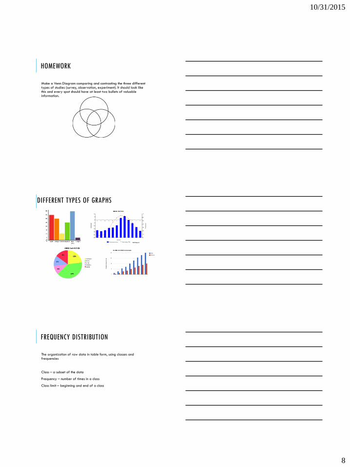
HOMEWORK
Make a Venn Diagram comparing and contrasting the three different types of studies (survey, observation, experiment). It should look like this and every spot should have at least two bullets of valuable information.
DIFFERENT TYPES OF GRAPHS
FREQUENCY DISTRIBUTION
The organization of raw data in table form, using classes and frequencies
Class – a subset of the data
Frequency – number of times in a class
Class limit – beginning and end of a class

10/31/2015
9
Suppose a researcher wants to do a study on the number of
miles that employees of Wal-Mart travel each day. She
collects the following data: (see data set 1)
1 2 6 7 12 13 2 6 9 5
18 7 3 15 15 4 17 1 14 5
5 16 4 5 8 6 5 18 5 2
9 11 12 1 9 2 10 11 4 10
9 18 8 8 4 14 7 3 2 6
1 2 6 7 12 13 2 6 9 5
18 7 3 15 15 4 17 1 14 5
5 16 4 5 8 6 5 18 5 2
9 11 12 1 9 2 10 11 4 10
9 18 8 8 4 14 7 3 2 6
Class limits Tally Frequency
1-3
4-6
7-9
10-12
13-15
16-18
1 2 6 7 12 13 2 6 9 5
18 7 3 15 15 4 17 1 14 5
5 16 4 5 8 6 5 18 5 2
9 11 12 1 9 2 10 11 4 10
9 18 8 8 4 14 7 3 2 6
Class limits Tally Frequency
1-3 ////’////’ 10
4-6 ////’////’//// 14
7-9 ////’////’ 10
10-12 ////’/ 6
13-15 ////’ 5
16-18 ////’ 5
10/31/2015
10
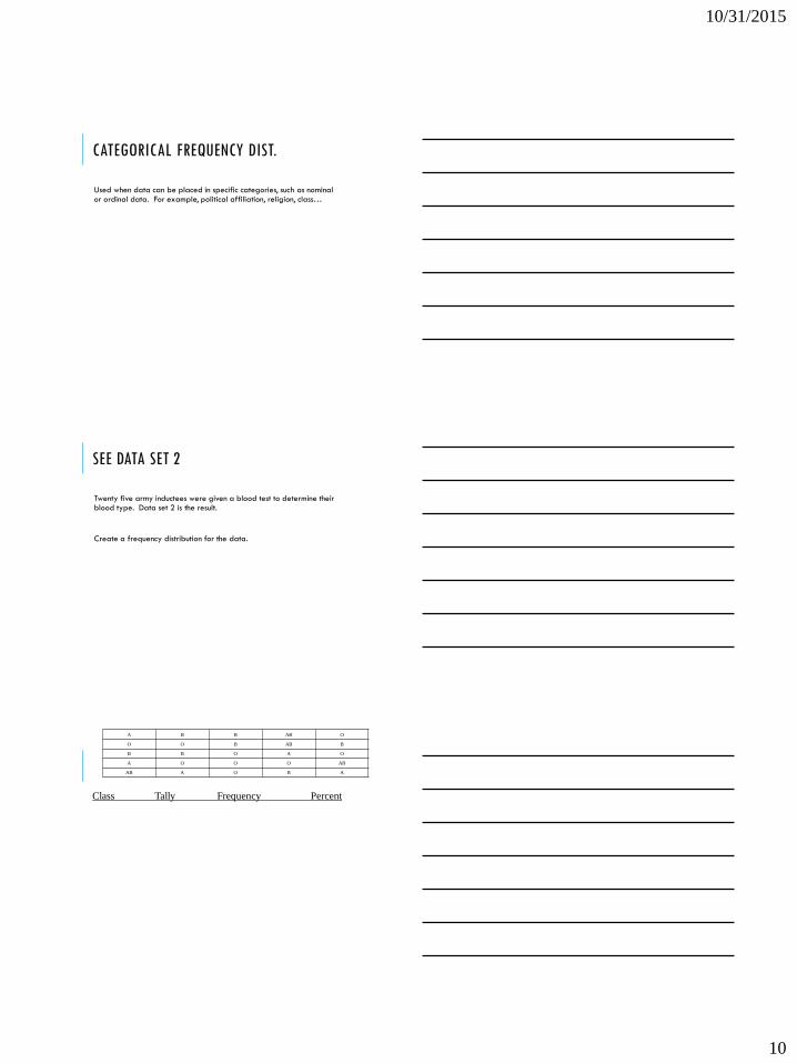
CATEGORICAL FREQUENCY DIST.
Used when data can be placed in specific categories, such as nominal or ordinal data. For example, political affiliation, religion, class…
SEE DATA SET 2
Twenty five army inductees were given a blood test to determine their blood type. Data set 2 is the result.
Create a frequency distribution for the data.
A B B AB O
O O B AB B
B B O A O
A O O O AB
AB A O B A
Class Tally Frequency Percent
10/31/2015
11
A B B AB O
O O B AB B
B B O A O
A O O O AB
AB A O B A
Class Tally Frequency Percent
A
B
O
AB
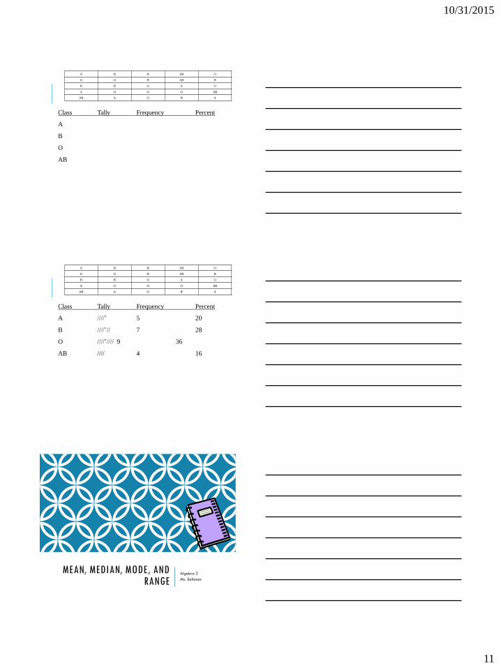
A B B AB O
O O B AB B
B B O A O
A O O O AB
AB A O B A
Class Tally Frequency Percent
A ////’ 5 20
B ////’// 7 28
O ////’//// 9 36
AB //// 4 16
MEAN, MEDIAN, MODE, AND RANGE
Algebra 2
Ms. Sellanes
10/31/2015
12
OBJECTIVE
Calculate and interpret the mean, median and mode of a set of data.
Central Tendency:
MEAN
Mean is the average of a set of data. To calculate the mean, find the sum of the data and then divide by the number of data.
Example: 12, 15, 11, 11, 7, 13
1. Add: 12 + 15 +11 + 11 + 7 + 13 = 69
2. How many datums? 6
3. Divide: Sum/(number of data)= 69/6
Conclusion: The mean or average is 11.5
An electronics store sells
CD players at the
following prices: $350,
$275, $500, $325, $100,
$375, and $300. What is
the mean price?
10/31/2015
13
An electronics store sells
CD players at the
following prices: $350,
$275, $500, $325, $100,
$375, and $300. What is
the mean price?
The mean or average price of a
CD player is $317.86.
MEDIAN
Median is the middle number in a set of data when the data is arranged in numerical order.
The median of a set of data separates the data into two equal parts.
Example: 12, 15, 11, 11, 7, 13
1. Arrange in Order: 7, 11, 11, 12, 13, 15
2. Find the middle number:
7, 11, 11, 12, 13, 15
3. If there are two numbers in the middle, take the average of the two number:
(11+12)/2=23/2=11.5
Conclusion: The mean or average is 11.5
YOUR TURN
An electronics store sells CD players at the following prices: $350, $275, $500, $325, $100, $375, and $300. What is the median price?
The median price is $325
10/31/2015
14
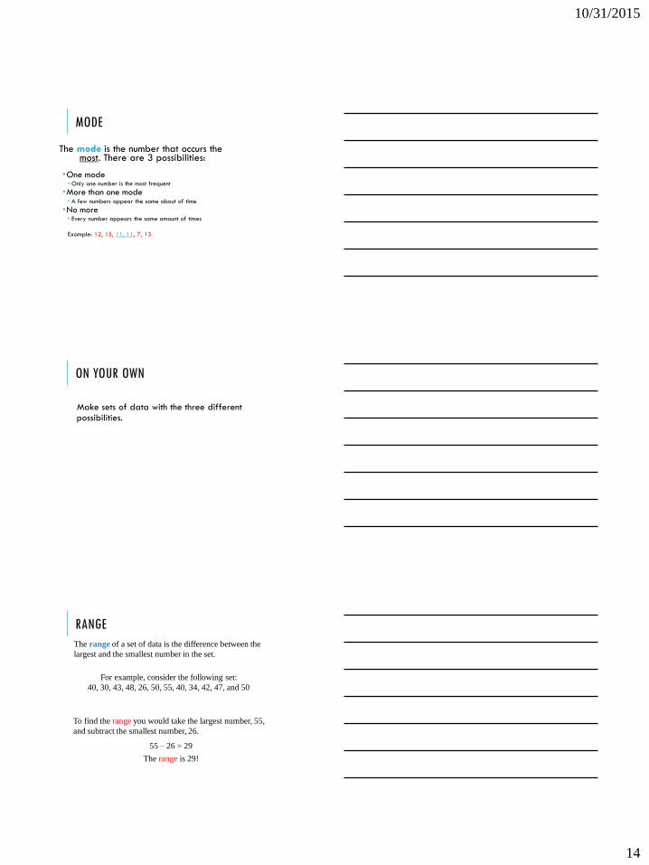
MODE
The mode is the number that occurs themost. There are 3 possibilities:
One mode Only one number is the most frequent
More than one mode A few numbers appear the same about of time
No more Every number appears the same amount of times
Example: 12, 15, 11, 11, 7, 13
ON YOUR OWN
Make sets of data with the three different possibilities.
The range of a set of data is the difference between the
largest and the smallest number in the set.
For example, consider the following set:
40, 30, 43, 48, 26, 50, 55, 40, 34, 42, 47, and 50
To find the range you would take the largest number, 55,
and subtract the smallest number, 26.
55 – 26 = 29
The range is 29!
RANGE
10/31/2015
15
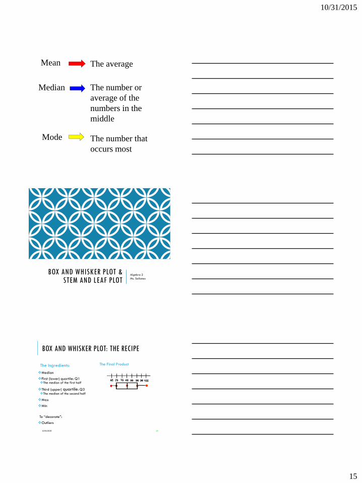
Mean The average
Median The number or
average of the
numbers in the
middle
Mode The number that
occurs most
BOX AND WHISKER PLOT & STEM AND LEAF PLOT
Algebra 2
Ms. Sellanes
BOX AND WHISKER PLOT: THE RECIPE
The Ingredients:
Median
First (lower) quartile: Q1The median of the first half
Third (upper) quartile: Q3The median of the second half
Max
Min
To “decorate”:
Outliers
The Final Product
10/31/2015 45

10/31/2015
16
GATHERING THE INGREDIENTS:
10/31/2015 46
Write the data in numerical
order and find the first quartile,
the median, the third quartile,
the smallest value and the
largest value.
median = 80
first quartile = 70
third quartile = 90
smallest value = 65
largest value = 100
DIRECTIONS
10/31/2015 47
Place a circle
beneath each
of these
values on a
number line.
DIRECTIONS
10/31/2015 48
Draw a box with ends
through the points for
the first and third
quartiles. Then draw
a vertical line through
the box at the median
point. Now, draw the
whiskers (or lines)
from each end of the
box to the smallest
and largest values.

10/31/2015
17
SPECIAL CASE:
10/31/2015 49
You may see a box-and-whisker plot, like the one
below, which contains an asterisk.
Sometimes there is ONE piece of data that falls well outside the
range of the other values. This single piece of data is called an
outlier. If the outlier is included in the whisker, readers may think
that there are grades dispersed throughout the whole range from
the first quartile to the outlier.
EXAMPLE
82 77 49 84 44 98 93
71 76 65 89 95 78 69
89 64 88 54 87 91 80
44 85 93 89 55 62 79
90 86 75 74 99 62 9610/31/2015 50
In pairs, you will make a box plot of the following data set.
That’s a lot of numbers so FIRST, let’s order the numbers with a stem-and-leaf plot
STEM-AND-LEAF PLOT
Stem Leaf
4 4 4 9
5 4 5
6 2 2 4 5 9
7 1 4 5 6 7 8 9
8 0 2 4 5 6 7 8 9 9 9
9 0 2 3 3 5 6 8 9
10/31/2015 51
8|2 represents a score of 82
10/31/2015
18
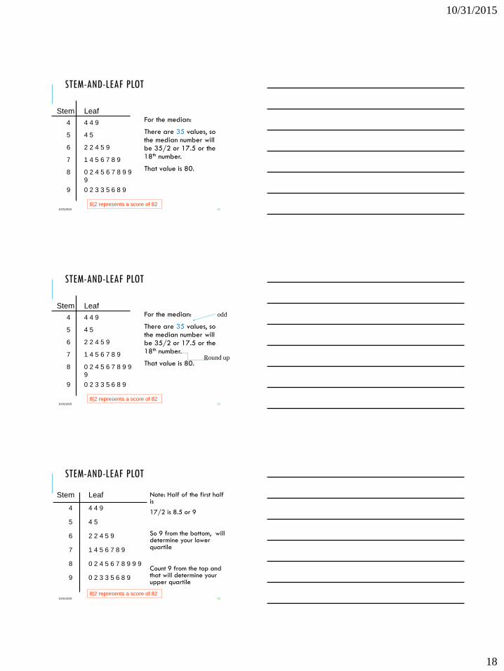
STEM-AND-LEAF PLOT
Stem Leaf
4 4 4 9
5 4 5
6 2 2 4 5 9
7 1 4 5 6 7 8 9
8 0 2 4 5 6 7 8 9 9
9
9 0 2 3 3 5 6 8 9
For the median:
There are 35 values, so the median number will be 35/2 or 17.5 or the 18th number.
That value is 80.
10/31/2015 52
8|2 represents a score of 82
STEM-AND-LEAF PLOT
Stem Leaf
4 4 4 9
5 4 5
6 2 2 4 5 9
7 1 4 5 6 7 8 9
8 0 2 4 5 6 7 8 9 9
9
9 0 2 3 3 5 6 8 9
For the median:
There are 35 values, so the median number will be 35/2 or 17.5 or the 18th number.
That value is 80.
10/31/2015 53
8|2 represents a score of 82
odd
Round up
STEM-AND-LEAF PLOT
Stem Leaf
4 4 4 9
5 4 5
6 2 2 4 5 9
7 1 4 5 6 7 8 9
8 0 2 4 5 6 7 8 9 9 9
9 0 2 3 3 5 6 8 9
Note: Half of the first half is
17/2 is 8.5 or 9
So 9 from the bottom, will determine your lower quartile
Count 9 from the top and that will determine your upper quartile
10/31/2015 54
8|2 represents a score of 82
10/31/2015
19
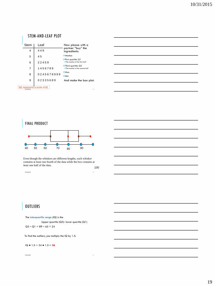
STEM-AND-LEAF PLOT
Stem Leaf
4 4 4 9
5 4 5
6 2 2 4 5 9
7 1 4 5 6 7 8 9
8 0 2 4 5 6 7 8 9 9 9
9 0 2 3 3 5 6 8 9
Now please with a partner “buy” the ingredients:
Median
First quartile: Q1The median of the first half
Third quartile: Q3The median of the second half
Max
Min
And make the box plot.
10/31/2015 55
8|2 represents a score of 82
FINAL PRODUCT
10/31/2015 56
40 50 60 70 80 90
100
Even though the whiskers are different lengths, each whisker
contains at least one fourth of the data while the box contains at
least one half of the data.
OUTLIERS
The interquartile range (IQ) is the
Upper quartile (Q3)- lower quartile (Q1)
Q3 – Q1 = 89 – 65 = 24
To find the outliers, you multiply the IQ by 1.5:
IQ ● 1.5 = 24 ● 1.5 = 36
10/31/2015 57
10/31/2015
20
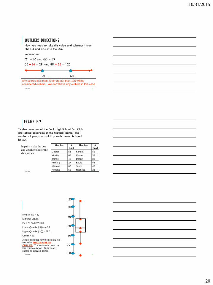
OUTLIERS DIRECTIONS Now you need to take this value and subtract it from the LQ and add it to the UQ.
Remember:
Q1 = 65 and Q3 = 89
65 – 36 = 29 and 89 + 36 = 125
10/31/2015 58
29 125
Any scores less than 29 or greater than 125 will be
considered outliers. We don’t have any outliers in this case
EXAMPLE 2
Member #
Sold
Member #
Sold
George 51 Kendra 55
Vinette 69 Carmen 39
Tomas 46 Danny 81
Anthony 27 Eddie 54
Marlene 60 Jason 46
Kohana 53 Nashoba 2310/31/2015 59
Twelve members of the Beck High School Pep Club are selling programs of the football game. The number of programs sold by each person is listed below:
In pairs, make the box
and whisker plot for the
data shown.
10/31/2015 60
30
20
40
50
60
70
80
Median (M) = 52
Extreme Values
LV = 23 and GV = 80
Lower Quartile (LQ) = 42.5
Upper Quartile (UQ) = 57.5
Outlier = 81
A point is plotted for 69 since it is the
last value THAT IS NOT AN
OUTLIER. The whisker is drawn to
this point as shown. Outliers are
plotted as isolated points.
10/31/2015
21
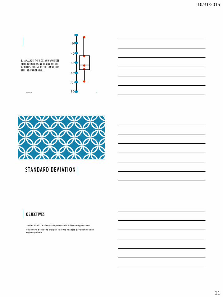
B. ANALYZE THE BOX-AND-WHISKER PLOT TO DETERMINE IF ANY OF THE MEMBERS DID AN EXCEPTIONAL JOB SELLING PROGRAMS.
10/31/2015 61
30
40
50
60
70
80
STANDARD DEVIATION
OBJECTIVES
Student should be able to compute standard deviation given data.
Student will be able to interpret what the standard deviation means in a given problem.
10/31/2015
22
INTRODUCTION
Consider two students, each of whom has taken five exams.
Student A has scores 84, 86, 83, 85, and 87.
Student B has scores 90, 75, 94, 68, and 98.
Compute the mean for both Student A and Student B
COMPUTING THE MEAN
85
5
425
5
9868947590
85
5
425
5
8785838684
x
x
x
x
x
xThe mean for Student A is 85
The mean for Student B is 85
AND . . .
For each of these students, the mean (average) of 5 tests is 85. However, Student A has a more consistent record of scores than Student B. One way to measure the consistency or “clustering” of data near the mean is the standard deviation.
10/31/2015
23
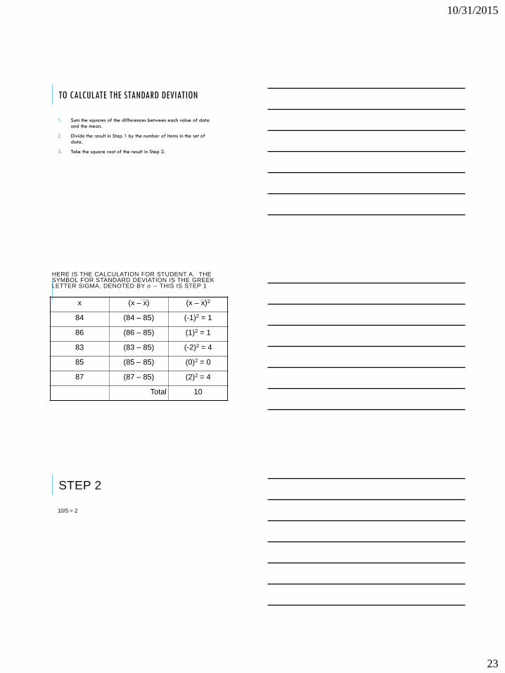
TO CALCULATE THE STANDARD DEVIATION
1. Sum the squares of the differences between each value of data and the mean.
2. Divide the result in Step 1 by the number of items in the set of data.
3. Take the square root of the result in Step 2.
HERE IS THE CALCULATION FOR STUDENT A. THE SYMBOL FOR STANDARD DEVIATION IS THE GREEK LETTER SIGMA, DENOTED BY -- THIS IS STEP 1
x (x – x) (x – x)2
84 (84 – 85) (-1)2 = 1
86 (86 – 85) (1)2 = 1
83 (83 – 85) (-2)2 = 4
85 (85 – 85) (0)2 = 0
87 (87 – 85) (2)2 = 4
Total 10
STEP 2
10/5 = 2
10/31/2015
24
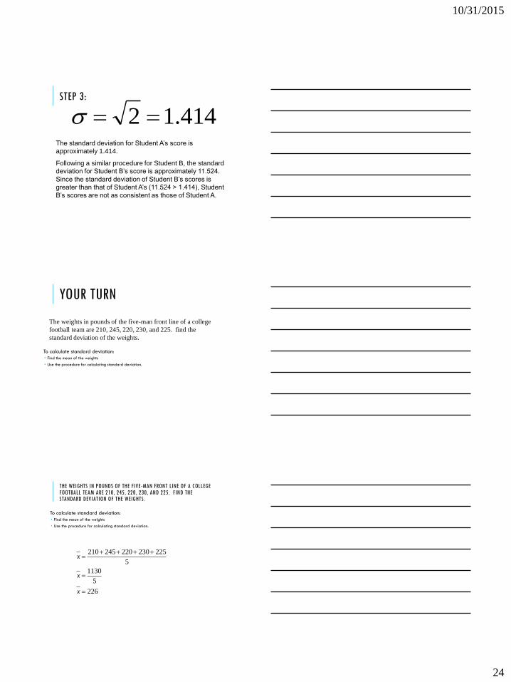
STEP 3:
414.12 The standard deviation for Student A’s score is
approximately 1.414.
Following a similar procedure for Student B, the standard
deviation for Student B’s score is approximately 11.524.
Since the standard deviation of Student B’s scores is
greater than that of Student A’s (11.524 > 1.414), Student
B’s scores are not as consistent as those of Student A.
YOUR TURN
To calculate standard deviation:
Find the mean of the weights
Use the procedure for calculating standard deviation.
The weights in pounds of the five-man front line of a college
football team are 210, 245, 220, 230, and 225. find the
standard deviation of the weights.
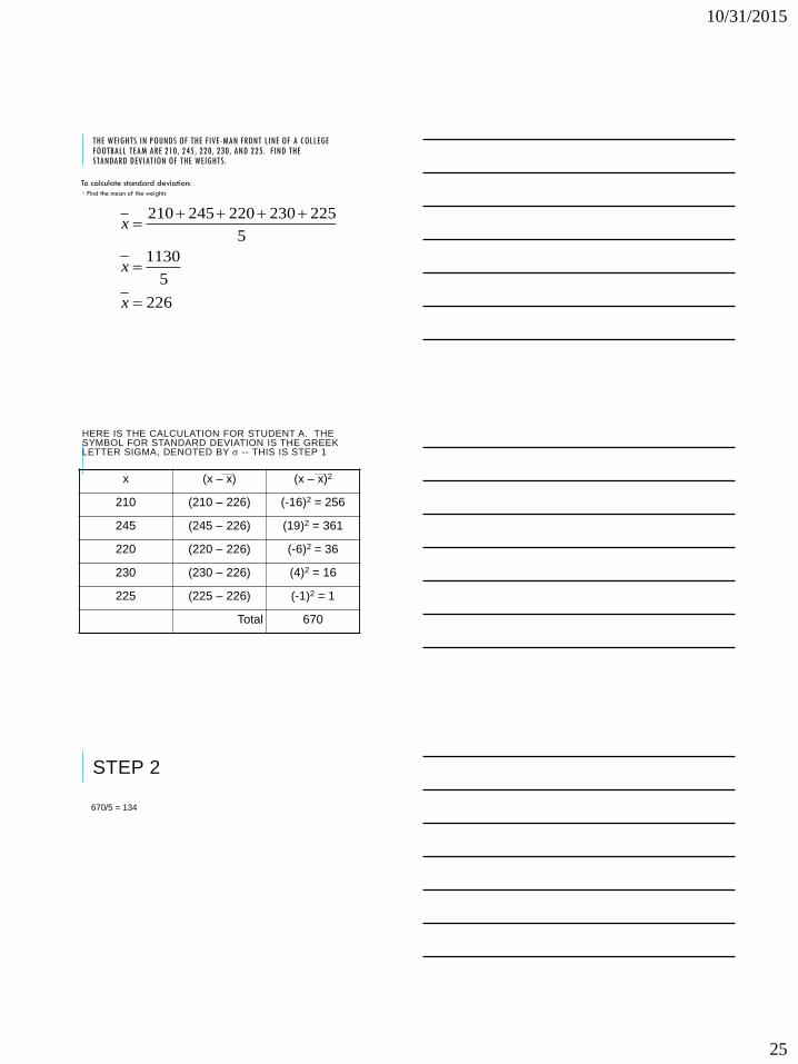
THE WEIGHTS IN POUNDS OF THE FIVE-MAN FRONT LINE OF A COLLEGE FOOTBALL TEAM ARE 210, 245, 220, 230, AND 225. FIND THE STANDARD DEVIATION OF THE WEIGHTS.
To calculate standard deviation:
Find the mean of the weights
Use the procedure for calculating standard deviation.
226
5
1130
5
225230220245210
x
x
x
10/31/2015
25
THE WEIGHTS IN POUNDS OF THE FIVE-MAN FRONT LINE OF A COLLEGE FOOTBALL TEAM ARE 210, 245, 220, 230, AND 225. FIND THE STANDARD DEVIATION OF THE WEIGHTS.
To calculate standard deviation:
Find the mean of the weights
226
5
1130
5
225230220245210
x
x
x
HERE IS THE CALCULATION FOR STUDENT A. THE SYMBOL FOR STANDARD DEVIATION IS THE GREEK LETTER SIGMA, DENOTED BY -- THIS IS STEP 1
x (x – x) (x – x)2
210 (210 – 226) (-16)2 = 256
245 (245 – 226) (19)2 = 361
220 (220 – 226) (-6)2 = 36
230 (230 – 226) (4)2 = 16
225 (225 – 226) (-1)2 = 1
Total 670
STEP 2
670/5 = 134

10/31/2015
26
576.11134 The standard deviation of the weights is approximately
11.576 lb.
NORMAL DISTRIBUTION
DIFFERENT SHAPES OF DISTRIBUTIONS
Distributions can be described as:
Roughly symmetric
Skewed right
Skewed left

10/31/2015
27
DISTRIBUTIONS OF DATAA distribution of data shows the observed or theoretical frequency of each possible data value.
Shape Definitions:
Symmetric: if the right and left sides of the graph are approximately mirror
images of each other.
Skewed to the right (right-skewed) if the right side of the graph is much longer
than the left side.
Skewed to the left (left-skewed) if the left side of the graph is much longer
than the right side.
Symmetric Skewed-left Skewed-right
10/31/2015
28
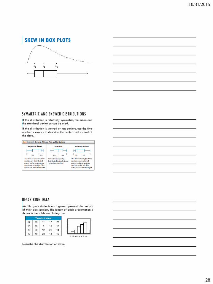
SKEW IN BOX PLOTS
SYMMETRIC AND SKEWED DISTRIBUTIONS
If the distribution is relatively symmetric, the mean and the standard deviation can be used.
If the distribution is skewed or has outliers, use the five-number summary to describe the center and spread of the data.
DESCRIBING DATA
Ms. Shroyer’s students each gave a presentation as part of their class project. The length of each presentation is shown in the table and histogram.
Describe the distribution of data.

10/31/2015
29
DESCRIBING DATADescribe the center of spread using either the mean and standard deviation or the five-number summary. Justify your choice.
COMPARING DATAThee points scored per game by a professional football team for the 2008 and 2009 football seasons are shown.
Create a box-and-whisker plot for each set. Describe the shape of each distribution. Then compare the distributions using either the means and standard deviations or the five-number summaries. Justify your choice.
COMPARING DATA
10/31/2015
30
COMPARING DATAThe lower quartile for the 2008 season and the upper quartile for the 2009 season are both 20.5. This means that 75% of the scores from 2008 were greater than 20.5 and 75% of the score from the 2009 season were less than 20.5
The minimum score of the 2008 season is approximately equal to the lower quartile for the 2009 season. This means that 25% of the scores from the 2009 season are lower than any score achieved in the 2008 season.
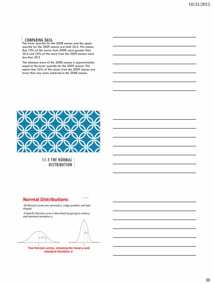
11-5 THE NORMAL DISTRIBUTION
Normal DistributionsAll Normal curves are symmetric, single-peaked, and bell-
shaped
A Specific Normal curve is described by giving its mean µand standard deviation σ.
Two Normal curves, showing the mean µ and
standard deviation σ.
10/31/2015
31
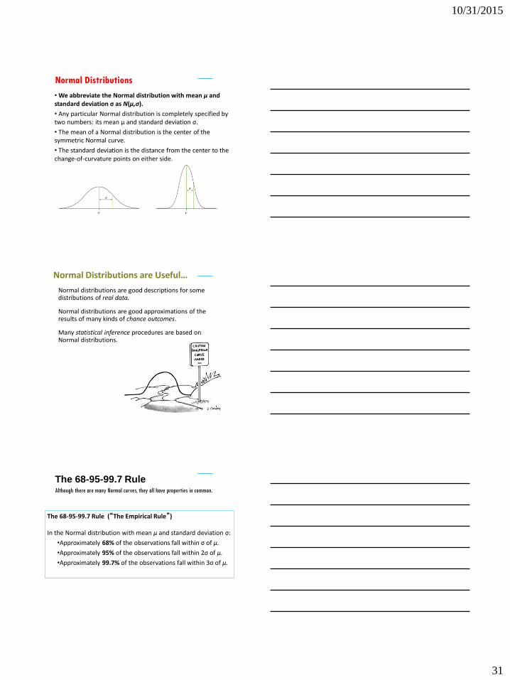
Normal Distributions
• We abbreviate the Normal distribution with mean µ and standard deviation σ as N(µ,σ).
• Any particular Normal distribution is completely specified by two numbers: its mean µ and standard deviation σ.
• The mean of a Normal distribution is the center of the symmetric Normal curve.
• The standard deviation is the distance from the center to the change-of-curvature points on either side.
Normal Distributions are Useful…
Normal distributions are good descriptions for some distributions of real data.
Normal distributions are good approximations of the results of many kinds of chance outcomes.
Many statistical inference procedures are based on Normal distributions.
Although there are many Normal curves, they all have properties in common.
The 68-95-99.7 Rule
The 68-95-99.7 Rule (“The Empirical Rule”)
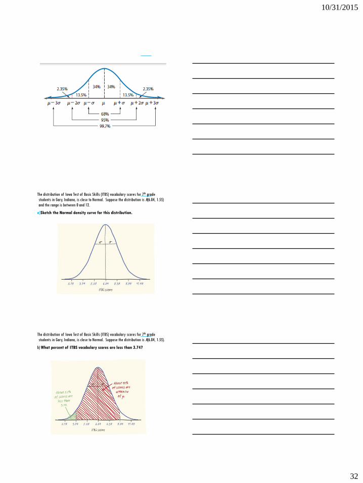
In the Normal distribution with mean µ and standard deviation σ:
•Approximately 68% of the observations fall within σ of µ.
•Approximately 95% of the observations fall within 2σ of µ.
•Approximately 99.7% of the observations fall within 3σ of µ.
10/31/2015
32
The distribution of Iowa Test of Basic Skills (ITBS) vocabulary scores for 7th grade
students in Gary, Indiana, is close to Normal. Suppose the distribution is N(6.84, 1.55)
and the range is between 0 and 12.
a)Sketch the Normal density curve for this distribution.
The distribution of Iowa Test of Basic Skills (ITBS) vocabulary scores for 7th grade
students in Gary, Indiana, is close to Normal. Suppose the distribution is N(6.84, 1.55).
b) What percent of ITBS vocabulary scores are less than 3.74?
10/31/2015
33
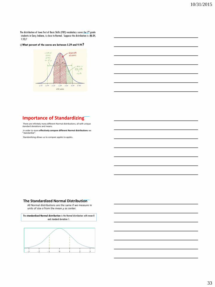
The distribution of Iowa Test of Basic Skills (ITBS) vocabulary scores for 7th grade
students in Gary, Indiana, is close to Normal. Suppose the distribution is N(6.84,
1.55).?
c) What percent of the scores are between 5.29 and 9.94?
Importance of Standardizing There are infinitely many different Normal distributions; all with unique standard deviations and means.
In order to more effectively compare different Normal distributions we “standardize”.
Standardizing allows us to compare apples to apples.
The Standardized Normal DistributionAll Normal distributions are the same if we measure in units of size σ from the mean µ as center.
The standardized Normal distribution is the Normal distribution with mean 0
and standard deviation 1.

10/31/2015
34
How to Standardize a Variable :
1. Draw and label an Normal curve with the mean and standard deviation.
2. Calculate the z- score
x= variable
µ= mean
σ= standard deviation
3. Determine the p-value by looking up the z-score in the Standard Normal table.
4. Conclude in context.
The Standard Normal Table
Because all Normal distributions are the same when we standardize, we can find areas under any Normal curve from a single table.
10/31/2015
35
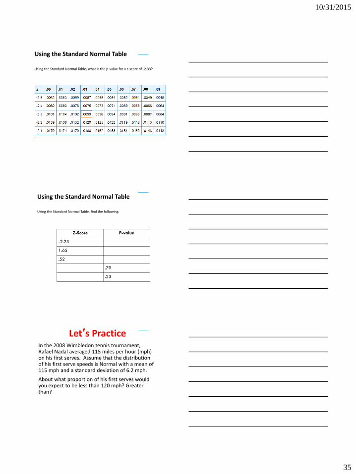
Using the Standard Normal Table
Using the Standard Normal Table, what is the p-value for a z-score of -2.33?
Using the Standard Normal Table
Using the Standard Normal Table, find the following:
Z-Score P-value
-2.23
1.65
.52
.79
.23
Let’s PracticeIn the 2008 Wimbledon tennis tournament, Rafael Nadal averaged 115 miles per hour (mph) on his first serves. Assume that the distribution of his first serve speeds is Normal with a mean of 115 mph and a standard deviation of 6.2 mph.
About what proportion of his first serves would you expect to be less than 120 mph? Greater than?
10/31/2015
36
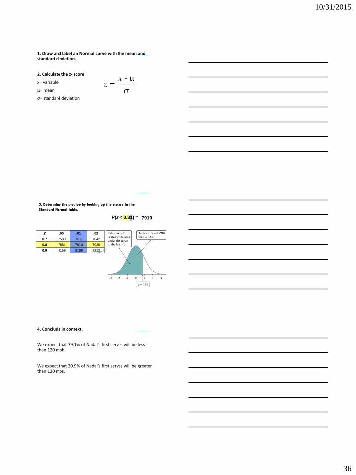
1. Draw and label an Normal curve with the mean and standard deviation.
2. Calculate the z- score
x= variable
µ= mean
σ= standard deviation
3. Determine the p-value by looking up the z-score in the
Standard Normal table.
Z .00 .01 .02
0.7 .7580 .7611 .7642
0.8 .7881 .7910 .7939
0.9 .8159 .8186 .8212
P(z < 0.81) = .7910
4. Conclude in context.
We expect that 79.1% of Nadal’s first serves will be less than 120 mph.
We expect that 20.9% of Nadal’s first serves will be greater than 120 mps.
10/31/2015
37
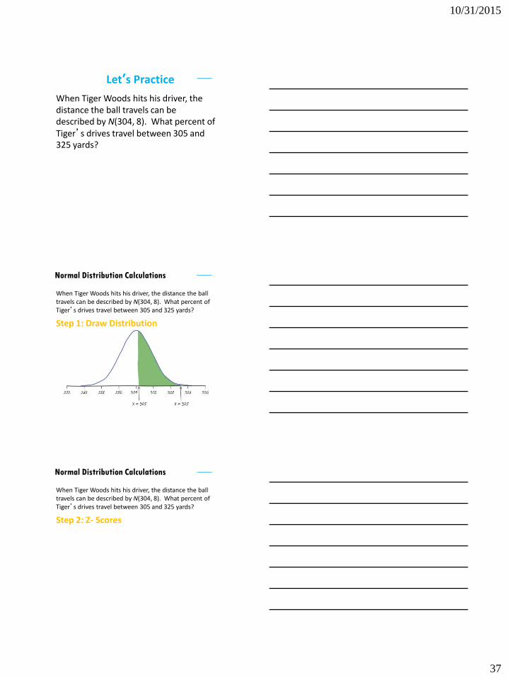
Let’s Practice
When Tiger Woods hits his driver, the distance the ball travels can be described by N(304, 8). What percent of Tiger’s drives travel between 305 and 325 yards?
Normal Distribution Calculations
When Tiger Woods hits his driver, the distance the ball travels can be described by N(304, 8). What percent of Tiger’s drives travel between 305 and 325 yards?
Step 1: Draw Distribution
Normal Distribution Calculations
When Tiger Woods hits his driver, the distance the ball travels can be described by N(304, 8). What percent of Tiger’s drives travel between 305 and 325 yards?
Step 2: Z- Scores
10/31/2015
38
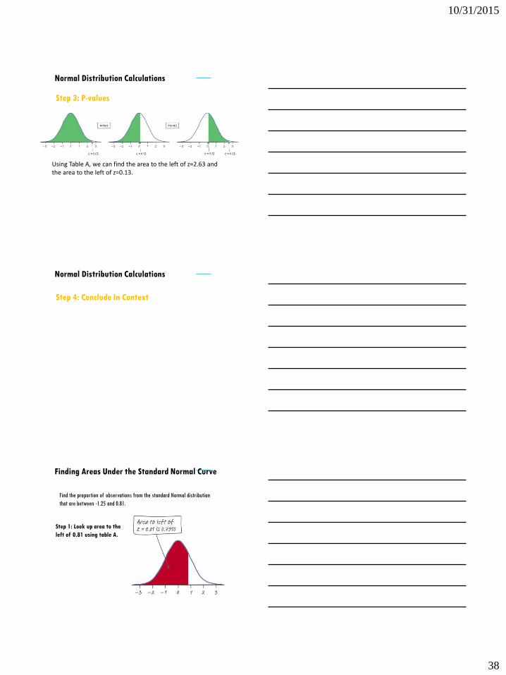
Normal Distribution Calculations
Step 3: P-values
Using Table A, we can find the area to the left of z=2.63 and the area to the left of z=0.13.
Normal Distribution Calculations
Step 4: Conclude In Context
Finding Areas Under the Standard Normal Curve
Find the proportion of observations from the standard Normal distribution
that are between -1.25 and 0.81.
Step 1: Look up area to the
left of 0.81 using table A.
10/31/2015
39
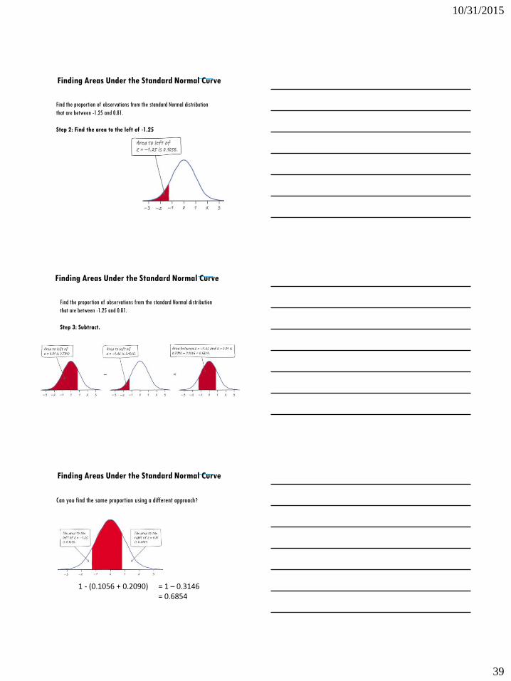
Finding Areas Under the Standard Normal Curve
Find the proportion of observations from the standard Normal distribution
that are between -1.25 and 0.81.
Step 2: Find the area to the left of -1.25
Finding Areas Under the Standard Normal Curve
Find the proportion of observations from the standard Normal distribution
that are between -1.25 and 0.81.
Step 3: Subtract.
Finding Areas Under the Standard Normal Curve
Can you find the same proportion using a different approach?
1 - (0.1056 + 0.2090) = 1 – 0.3146= 0.6854
10/31/2015
40
11-6 CONFIDENCE INTERVALS AND HYPOTHESIS TESTING
CONFIDENCE INTERVALS
Inferential statistics are used to draw conclusions or statistical inferences about a population using a sample.
Example: In a recent poll, 1514 teens who owned a portable media player had an average of 1033 songs. The poll had the following disclaimer: “For results based on the total sample of national teens, one can say with 95% confidence that the margin of sampling error is ±31 songs.
CONFIDENCE INTERVALS
Is an estimate of a population parameter stated as a range with a specific degree of certainty.
A 95% confidence interval for a population means that we are 95% sure that the mean will fall within the range of z-values.
Example: We were 95% confident that the population mean is within 31 songs of
1033.

10/31/2015
41
MAXIMUM ERROR OF ESTIMATE
MAXIMUM ERROR ESTIMATE EXAMPLEORAL HYGIENE A poll of 422 randomly selected adults showed that they brushed their teeth an average of 11.4 times per week with a standard deviation of 1.6. Use a 99% confidence interval to find the maximum error of estimate for the number of times per week adults brush their teeth.
MAXIMUM ERROR OF ESTIMATE CONT. Maximum Error of Estimate

10/31/2015
42
EXAMPLE
A. 0.49
B. 0.80
C. 0.96
D. 1.26
READING A poll of 385 randomly selected adults showed that they read for recreation an average of 39.3 minutes per week with a standard deviation of 9.6 minutes. Use a 95% confidence interval to find the maximum error of estimate for the number of minutes per week adults read for recreation.
CONFIDENCE INTERVAL FOR THE POPULATION MEAN
CONFIDENCE INTERVAL PACKAGING A poll of 156 randomly selected members of a golf course showed that they play an average of 4.6 times every summer with a standard deviation of 1.1. Determine a 95% confidence interval for the population mean.
Confidence Interval for
Population Mean