statistics and modelling course 2011. topic: sample statistics & expectation part of achievement...

Statistics and Modelling Course

2011

Topic: Sample statistics & expectation

Part of Achievement Standard 90643

Solve straightforward problems involving probability

4 CreditsExternally Assessed

NuLake Pages 147163 Sigma: Old version – Ch

2.New version – Ch 7.

LESSON 1 – Probability distribution

Points of today: Learn the meaning of discrete and continuous random variables. Use a probability distribution table to display outcomes. What is Expected Value and how do you calculate it?

1. Notes on discrete & continuous random variables.

2. Do old Sigma (2nd edition) – p23 – Ex. 2.1

3. Notes on probability distribution tables (handout to fill in).

4. Introduction to Expected Value.

Discrete and Continous data

Discrete Continuous


Discrete ContinuousWhere does its value come from?



Counting



Counting Measurement




What values can it take?





Whole numbers or rounded values






All real numbers (anywhere along the number line – infinite precision)







What question is being asked?








‘How many ?’








‘How many ?’ ‘How long ?’, ‘ How heavy ?’









Examples:









Examples:• Number of students who gained Excellence in last test.• Money – if to the nearest dollar/cent.









Examples:• Number of students who gained Excellence in last test.• Money – if to the nearest dollar/cent.

• Height• Distance• Weight• Volume• Time

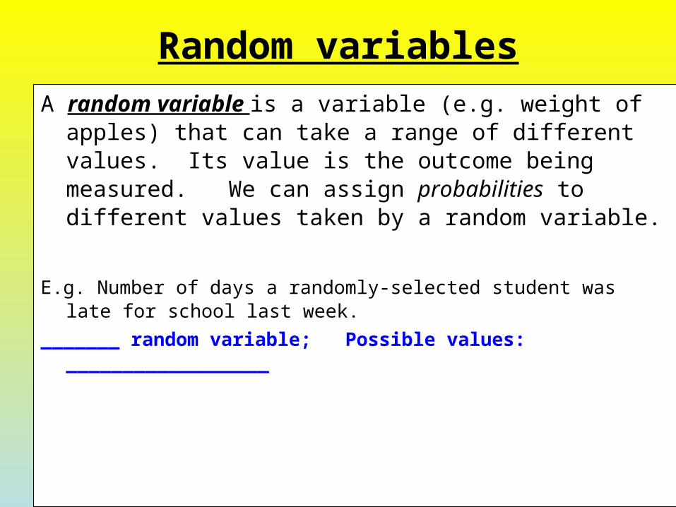
Random variablesA random variable is a variable (e.g. weight of

apples) that can take a range of different values.


apples) that can take a range of different values. Its value is the outcome being measured.


apples) that can take a range of different values. Its value is the outcome being measured. We can assign probabilities to different values taken by a random variable.

E.g. Number of days a randomly-selected student was late for school last week.

_______ random variable; Possible values: __________________




Discrete random variable; Possible values: __________________




Discrete random variable; Possible values: 0, 1, 2, 3, 4, 5.

E.g. A poll of 1000 voters to see who favours John Key as P.M.

_______ random variable; Possible values: __________________






Discrete random variable; Possible values: __________________

Random variablesA random variable is a variable (e.g. weight of apples)

that can take a range of different values. Its value is the outcome being measured. We can assign probabilities to different values taken by a random variable.




Discrete random variable; Possible values: 0, 1, 2,……, 999, 1000

E.g. The volume of tomato sauce in a bottle – varies slightly.

__________random variable; Values will be ________________.








Continuous random variable; Values will be ________________.








Continuous random variable; Values will be positive real numbers.








Continuous random variable; Values will be positive real numbers.

Do Sigma p23 – Ex. 2.1 – Just Q19, and 13 if you’re fast.

In new Sigma: p121 – Ex. 7.01 – all qs.

Probability Distributions - fill in notes on handout

Probability DistributionsSurvey: How many ‘children’ in your family?

Let x represent ‘number of children in family’.

Probability DistributionsSurvey: How many ‘children’ in your family?

Let x represent ‘number of children in family’. x 1 2 3 4 5 6 7

Frequency

Relativefrequency

n

f

Survey: How many ‘children’ in your family?

Let x represent ‘number of children in family’.

And: probability = long-run relative frequency.So we can draw a Probability Distribution table from this data:

x 1 2 3 4 5 6 7

Frequency

Relativefrequency

n

f

x 1 2 3 4 5 6 7

P(X = x)

Calculate the mean number of kids per family in this class…

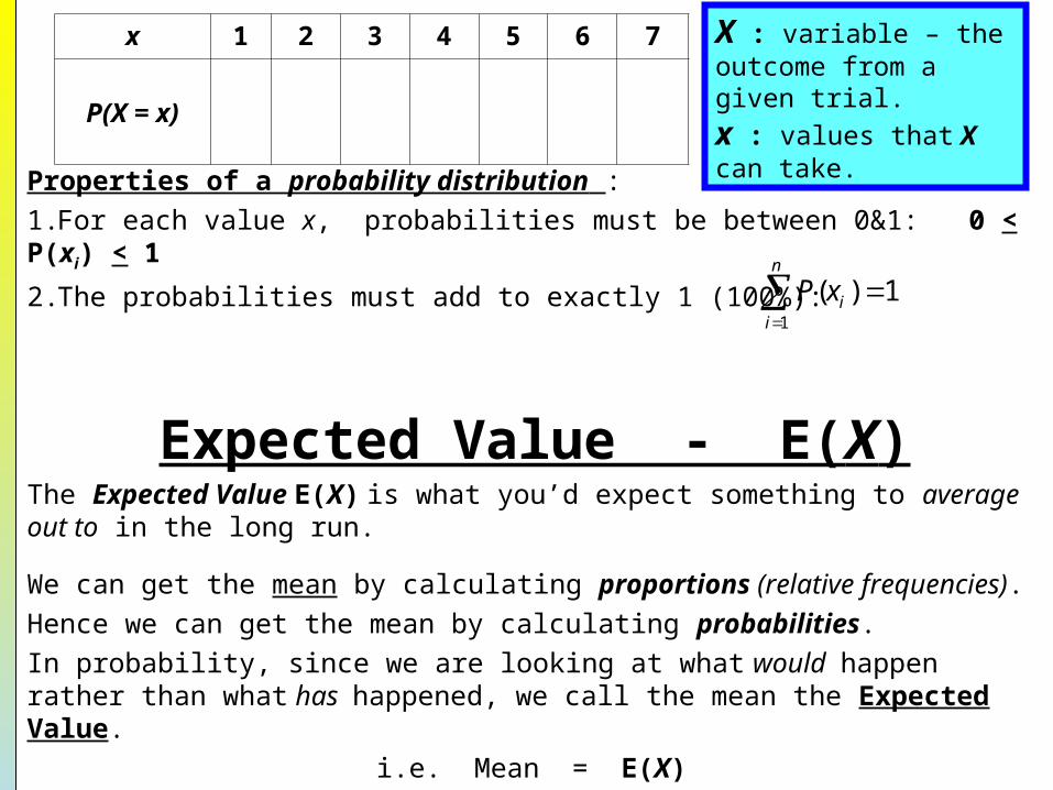
X : variable – the outcome from a given trial.x : values that X can take.

Survey: How many ‘children’ in your family?

Let x represent ‘number of children in family’. .


Properties of a probability distribution :1.For each value x, probabilities must be between 0&1: 0 < P(xi) < 1

2.The probabilities must add to exactly 1 (100%):

x 1 2 3 4 5 6 7

Frequency

Relativefrequency

n

f

x 1 2 3 4 5 6 7

P(X = x)

n

iixP

1

1)(




2.The probabilities must sumto exactly 1 (100%):

Expected Value - E(X)The Expected Value E(X) is what you’d expect something to average out to in the long run.

x 1 2 3 4 5 6 7

P(X = x)

n

iixP

1

1)(





We can get the mean by calculating proportions (relative frequencies).Hence we can get the mean by calculating probabilities.

x 1 2 3 4 5 6 7

P(X = x)

n

iixP

1

1)(





We can get the mean by calculating proportions (relative frequencies).Hence we can get the mean by calculating probabilities.In probability, since we are looking at what would happen rather than what has happened, we call the mean the Expected Value.

i.e. Mean = E(X)

x 1 2 3 4 5 6 7

P(X = x)

n

iixP

1

1)(


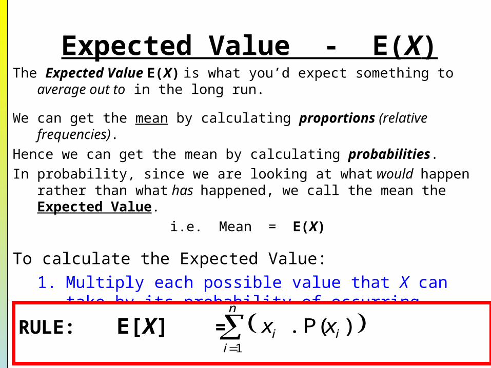
Expected Value - E(X)The Expected Value E(X) is what you’d expect something to

average out to in the long run.

We can get the mean by calculating proportions (relative frequencies).

Hence we can get the mean by calculating probabilities.In probability, since we are looking at what would happen rather

than what has happened, we call the mean the Expected Value.

i.e. Mean = E(X)

To calculate the Expected Value:1. Multiply each possible value that X can take by its

probability of occurring.2. The sum of all of these gives the Expected Value

of X.RULE: E[X] =

n

iii xx

1

)P( .

We can get the mean by calculating proportions (relative frequencies).Hence we can get the mean by calculating probabilities.In probability, since we are looking at what would happen rather than what has happened, we call the mean the Expected Value.

i.e. Mean = E(X)


probability of occurring.2. The sum of all of these gives the Expected Value

of X.RULE: E[X] =

n

iii xPx

1

)( .

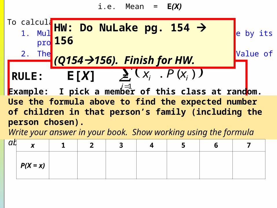
Example: I pick a member of this class at random. Use the formula above to find the expected number of children in that person’s family (including the person chosen).Write your answer in your book. Show working using the formula above.

i.e. Mean = E(X)


probability of occurring.2. The sum of all of these gives the Expected Value of X.

RULE: E[X] =

n

iii xPx

1

)( .

Example: I pick a member of this class at random. Use the formula above to find the expected number of children in that person’s family (including the person chosen).Write your answer in your book. Show working using the formula above.

x 1 2 3 4 5 6 7

P(X = x)

HW: Do NuLake pg. 154 156

(Q154156). Finish for HW.

LESSON 1A (if time) – Expected Value applications

Points of today: Calculate expected values. Calculate expected gains / losses when there is a price/reward

associated with the outcomes.

1. Go over a couple of the HW problems – NuLake p154 & 156.

2. Go through expected gain problem on the following slides

3. More practice of basics? Do Sigma (old) p25 – Ex. 2.2.

OR

Got it. Ready to do some more applications problems? Do Sigma (old) p26 – Ex. 2.3 – complete for HW.

7.03B A lottery has three prizes: $2000, $500 and $100. If there are 1300tickets, and assuming all tickets are sold, what should the organisercharge for each ticket if the lottery is to be ‘fair’?

Let x: expected winnings form 1 ticket.List the four possible outcomes for the buyer of one ticket


Win $2000

The four possible outcomes for the buyer of one ticket are:

Win $500Win $100Lose

Write down the amount the buyer wins each case.

Let x: expected winnings form 1 ticket.


Win $2000

0

Winnings= 2000500100


Express this as a probability distribution in a table.



Buyer’s winnings, x

2000 500 100 0

P(X = x)


Win $2000

0

Winnings = 2000500100


11300

11300

11300


As there 3 winning tickets, the number of losing tickets is 1297

12971300



11300

11300

11300

12971300

Write down an expression for the expected value.


2000 500 100 0

P(X = x)


11300

11300

11300

12971300

( )E X

If the lottery is fair the ticket price must be equal to the expected winnings per ticketet

i.e. on average, nobody gains and nobody loses


2000 500 100 0

P(X = x)

So the tickets should sell for $___


2000 500 100 0

P(X = x)


11300

11300

11300

12971300

( )E X

If the lottery is fair the ticket price must be equal to the expected winnings per ticketet

i.e. on average, nobody gains and nobody losesSo the tickets should sell for $2

Need more practice of the basics?Do Sigma (old) – pg. 25 – Ex. 2.2

Got it. Now ready to do more applied problems like this one: Do Sigma pg. 26 – Ex. 2.3.

LESSON 2 – Calculate the Variance from a probability distribution table 1

Points of today: Calculate the expected value of a function of a variable. Learn how to calculate the variance from a probability distribution

table.

1. Go over a couple of the HW problems – NuLake pg. 154156 (focus on application qs as this is the emphasis in NCEA).

2. Briefly go through how to calculate the expected value of a function of a variable – examples on next slide.

3. Notes on how to calculate the variance of a random variable (most of lesson).

4. Do NuLake pg. 158161 (finish for HW).

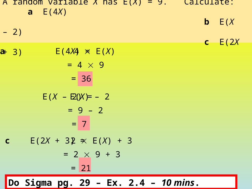
A random variable X has E(X) = 9. Calculate: a E(4X) b E(X – 2) c E(2X + 3)

4 E(X)

b E(X – 2) =

a E(4X) =

= 4 9

= 36

E(X) – 2

= 9 – 2

2 E(X) + 3

= 21

c E(2X + 3) =

= 2 9 + 3

= 7

Do Sigma pg. 29 – Ex. 2.4 – 10 mins.

Variance“The average of the squared distances

from the mean.”

Var(X) =

Var(X) = E[(X – μ)2]

This can be re-arranged to get

The same as saying the “Expected” squared distance from the population mean.

n

xx 2)(

Var(X) = E(X2) – [E(X)]

2


from the mean.”

Var(X) =

Var(X) = E[(X – μ)2]



n

xx 2)(

Var(X) = E(X2) – μ

2


from the mean.”

Var(X) =

Var(X) = E[(X – μ)2]



n

xx 2)(

Var(X) = E(X2) – [E(X)]

2

7.05DCalculate the mean, variance and standard deviation for this probability distribution. Use the formula VAR(X) = E(X2) – µ2 for the variance.

μ = E(X)= 26.7

= 102 0.18 + 202 0.32 + 302 0.15 + 402 0.35 = 18 + 128 + 135 + 560 = 841

Var(X) = E(X2) – µ2 = 841 – (26.7)2 = 128.11

= = 128.11

x 10 20 30 40

P(X = x) 0.18 0.32 0.15 0.35

= 10 0.18 + 20 0.32 + 30 0.15 + 40 0.35

E(X2)

= 11.32 (to 4SF)

Calculate E[X].

Calculate E[X2].

Use VAR(X) = E(X2) – µ2

to calculate the variance.

Hence calculate SD(X).

Do NuLake pg. 158 161

(Q164176). Finish for HW.

)(XVar

The mean, based on the above probability distribution, is μ = 26.7.

The variance, based on the above probability distribution, is 128.11

The standard deviation, based on the above probability distribution, is

σ = 11.32 (to 4 S.F.).

LESSON 3 – Calculate the Variance from a prob. distn.table 2

Point of today – practice!: Get confident at calculating the variance from a probability

distribution table.

1. Any Qs from the HW – NuLake – pg. 158161?

2. Another e.g. on board (following slides) for those needing it (others carry on).

3. Do Sigma: pg. 33 (Ex. 2.5) in old, or pg. 135 (Ex. 7.05) in new:

MUST do Q 1 & 2, (* 35 are optional as extension).

4. Then on to next exercise (2.6 in old / 7.06 in new): Do all. Complete for HW.


from the mean.”

Var(X) =

Var(X) = E[(X – )2]



n

xx 2)(

Var(X) = E(X2) – μ

2


from the mean.”

Var(X) =

Var(X) = E[(X – )2]



n

xx 2)(

Var(X) = E(X2) – [E(X)]

2

For the probability distribution table below:1.) Calculate the mean E(X) = .2.) Calculate 2

3.) Calculate E(X2).4.) Explain in your own words why E(X2) ≠ 2

5.) Use the formula VAR(X) = E(X2) – µ 2 to calculate the variance & standard deviation of X.

μ = E(X)

= 7.6

= 52 0.2 + 72 0.4 + 82 0.3 + 142 0.1

= 63.4Var(X) = E(X2) – µ2

= 63.4 – 7.62 = 5.64

x 5 7 8 14

P(X = x) 0.2 0.4 0.3 0.1

= 5 0.2 + 7 0.4 + 8 0.3 + 14 0.1

E(X2)

= 2.375 (4 S.F.)

Calculate E[X].

Now Calculate E[X2]. Use VAR(X) = E(X2) – µ2

to calculate the variance.Now calculate σ

(the Standard Deviation)

The variance, based on the above probability distribution, is σ2 = 5.64

)(XVar 64.5

The standard deviation, based on the above probability distribution, is

σ = 2.375 (4 S.F.).

The mean, based on the above probability

distribution, is μ = 7.6. So μ2 = 7.62 = ____

1. Finish NuLake pages 158161 (ask for help with any you’re stuck on.)

2. Do Sigma (old) pg. 33 – Ex. 2.5 – JUST Q1 & 2. (* Q35 are optional as extension).

3. Then on to Ex. 2.6 (pg. 34). Finish for HW.

Variance formula proof using Expectation:Link between the 2 variance formulas: Prove that =

Left hand side =

=

=

=

=

=

= Right hand side

2)( XE 22 )( XE

2)( XE

).2( 22 XXE

)()2()( 22 EXEXE

22 )(2)( XEXE Since E() = i.e. the expected value of the mean is the mean.

222 2)( XE Since E(X) =

22 )( XE

LESSON 4 – Variance of a function of a variable

Point of today: How to calculate the variance (and standard deviation) of a

function of a variable.

1. Notes & examples.

2. Do NuLake pg. 164 & 166.

3. Sigma (old – 2nd edition) – pg. 36: Ex. 2.7.

Linear Functions of Random Variables

Sometimes we deal with random variables whose behaviour is modelled by a linear function:

Y = aX +c(like y = mx + c)

E.g. A taxi service charges $3 per kilometer travelled plus a flat fee of $5.

If the distance, X, required for the next job is a random variable, then the price, Y, is given by Y = 3X+5

Its mean is given by E(3X + 5) = 3 × μ + 5


Sometimes we deal with random variables whose behaviour is modelled by a linear function:

Y = aX +c



Its mean is given by E(3X + 5) = 3 × E(X) + 5Its variance, Var(3X+5) =

Its std. deviation, σ3X+5 = )(32 XVar

32 × Var(X)




Its mean is given by E(3X + 5) = 3 × E(X) + 5Its variance, Var(3X+5) =

Its std. deviation, σ3X+5 =

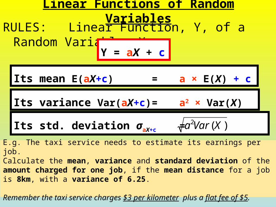
RULES: Linear Function, Y, of a Random Variable, X

)(32 XVar

32 × Var(X)

Y = aX + c

Its mean E(aX+c) = a × E(X) + c

Its variance Var(aX+c) = a2 × Var(X)

Its std. deviation σaX+c = )(2 XVara



Y = aX + c




E.g. The taxi service needs to estimate its earnings per job. Calculate the mean, variance and standard deviation of the amount charged for one job, if the mean distance for a job is 8km, with a variance of 6.25.



Y = aX + c





Remember the taxi service charges $3 per kilometer plus a flat fee of $5.



Let X: Distance for a job.Y: Price of a job.

μY = E(Y) =E(3X + 5) = 3× 8 + 5

= $29

= $7.50

So the mean price charged for a job is $29.

25.56

Then Y = 3X + 5

σ2Y = Var(Y) = Var(3X+5) = 32 6.25

= 56.25 So the random variable, Y (price charged) has avariance of 56.25and a std. deviation of $7.50.

σY =

•Do NuLake pg. 164-166•Then Sigma (old) – pg. 36

Further extension:Sigma (old): Ex. 2.7

LESSONS 5 & 6 – Sums & differences of 2 random variables

Point of today: How to calculate the mean, variance (and standard deviation) of

the sum of 2 independent random variables. How to calculate the mean, variance (and standard deviation) of

the difference between 2 independent random variables.

1. Warm-up quiz (re-cap from last lesson – function of a random variable).

2. Examples & notes.

3. Do NuLake pg. 168 (just Q187 & 188)

4. Then do Sigma (old – 2nd edition) – pg. 41: Ex. 2.9 (skip Q2).

5. Do Sigma (old – 2nd edition) – pg. 42 & 43: Ex. 2.10.

6. Extension: NuLake p169, 170: Questions 189-194 only.

WARM-UP QUIZ: X is a random variable with mean 20 and variance 2 = 16. Calculate the mean, variance and standard deviation of Y, if:a Y = 6Xb Y = 3X -4c Y = -X


Y = aX + c





μY = E(Y) = E(6X) = 6 E(X)

= 6 20

= 120

σ2Y = Var(Y) =Var(6X) = 62 Var(X)

= 36 16

= 576

σY =

= 24

Simply multiply E(X) by 6.

Square the coefficient of X.

Square root of the variance.

576


μY = E(Y) = E(3X - 4) = 3 E(X) - 4

= 320 - 4

= 56

σ2Y =Var(Y) =Var(3X - 4) = 32 Var(X)

= 9 16

= 144

σY =

= 12

Multiply E(X) by 3 and subtract 4.

Square the coefficient of X. IGNORE THE -4

Square root of the variance.

144

7.07WARM-UP QUIZ: X is a random variable with mean 20 and variance 2 = 16. Calculate the mean, variance and standard deviation of Y, if:a Y = 6Xb Y = 3X -4c Y = -X

μY = E(Y) = E(-X) = -1 E(X)

= -20

σ2Y = Var(Y) =Var(-X) = Var(X)

= 16

σY =

= 4

Simply multiply E(X) by -1.

This has no effect on the SPREAD of the data.

So of course the standard deviation is also unchanged.

16

E.g. 1. The mean weight of Year 13 males at a school is 72Kg with a standard deviation of 5Kg. The mean weight of Year 13 females at the same school is 56Kg with a standard deviation of 4Kg.One boy and one girl are chosen at random and their individual weights are added together.What would be the mean, variance and standard deviation of their combined weight?

SUMS OF 2 INDEPENDENT RANDOM VARIABLES

Distribution of X + Y

Its mean E(X + Y) = E(X) + E(Y)

Its variance Var(X + Y) = Var(X) + Var(Y)

Its std. deviation σX+Y = )()( YVarXVar


Let T: Combined Weight; X: Weight of a randomly chosen boy.Y: Weight of a randomly chosen girl.

Where T = X + Y

μT = E(T) = E(X+Y) = E(X) + E(Y)

5672 kg128

Var(T) = Var(X)+Var(Y)

= 52 + 42 Always work through the variances rather than the standard deviations.We square the boys’ and girls’ standard deviations to get their variances.

Assumption: That the marks for the 2 tests are independent.Then we can add the variances.


Let T: Combined Weight; X: Weight of a randomly chosen boy.Y: Weight of a randomly chosen girl.

Where T = X + Y

μT = E(T) = E(X+Y) = E(X) + E(Y)

5672 kg128

Var(T) = Var(X)+Var(Y)

= 52 + 42

So, assuming that the weights of boys and girls are independent, we would expect the combined weight of a randomly chosen boy & girl to be 128kg, with a standard deviation of 6.403kg (4sf).

= 41

)(TVarT 41 = 6.403kg (4sf)

We SUBTRACT the MEANS, but still ADD the VARIANCES.

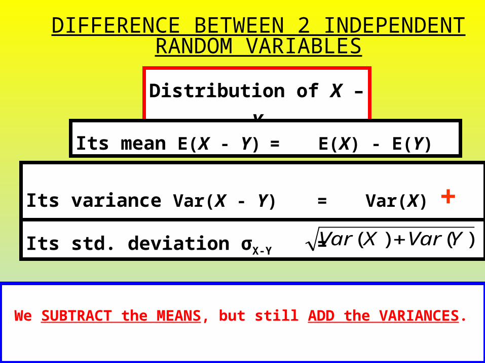
DIFFERENCE BETWEEN 2 INDEPENDENT RANDOM VARIABLES

Distribution of X – Y

Its mean E(X - Y) = E(X) - E(Y)

Its variance Var(X - Y) = Var(X) + Var(Y)

Its std. deviation σX-Y = )()( YVarXVar

We SUBTRACT the MEANS, but still ADD the VARIANCES.

Its mean E(X - Y) = E(X) - E(Y)

Its variance Var(X - Y) = Var(X) + Var(Y)

Its std. deviation σX-Y = )()( YVarXVar

The contents of a tin of cat food have a distribution with mean 500 g and standard deviation 6 g. A spoon is used to remove the food from the tin. The amount of food removed has a distribution with mean 60 g and standard deviation 4 g. Calculate the mean and standard deviation of the amount of food left in the tin after one spoonful is removed.

7.09

The contents of a tin of cat food have a distribution with mean 500 g and standard deviation 6 g. A spoon is used to remove the food from the tin. The amount of food removed has a distribution with mean 60 g and standard deviation 4 g. Calculate the mean and standard deviation of the amount of food left in the tin after one spoonful is removed.

7.09

Let the random variables involved beX = volume of tin contentsY = volume on spoon

Write an expression for the volume of food left in the tin once the spoonful is removed.

The contents of a tin of cat food have a distribution with mean 500 g and standard deviation 6 g. A spoon is used to remove the food from the tin. The amount of food removed has a distribution with mean 60g and standard deviation 4g. Calculate the mean and standard deviation of the amount of food left in the tin after one spoonful is removed.

7.09

Let the random variables involved beX = volume of tin contentsY = volume on spoonX–Y = volume of cat food remaining in tin.

Calculate the expected volume of cat food remaining – i.e. E[X–Y].


7.09

E(X) – E(Y)

= 500 – 60

= 440 g

E(X–Y) =

Mean = expected value

So the mean volume remaining is 440g.


Calculate Var(X–Y).


7.09

E(X) – E(Y)

= 500 – 60

= 440 g

E(X–Y) =



X = volume of tin contentsY = volume on spoonX–Y = volume of cat food remaining in tin.

Calculate σX–Y


7.09

Let the random variables involved be

E(X) – E(Y)

= 500 – 60

Var(X) + Var(Y)

= 62 + 42

= 52

Var(X–Y) =

= 440 g

E(X–Y) =




E(X) – E(Y)

= 500 – 60

E(X–Y) =

Var(X) + Var(Y)

= 62 + 42

= 52

Var(X–Y) =

σX–Y =

= 7.211 g (4 sf)

52


7.09

= 440 g

•Do NuLake pg. 169 (Q187, 188 only)•Then Sigma (old) – pg. 41Ex. 2.9 (skip Q2) – FINISH FOR HW



So the standard deviation of the remaining volume is 7.211g (4SF).

Extension work– Linear combinations of 2 random variables

Point of today: How to calculate the mean, variance (and standard deviation) of a

linear combination of 2 independent random variables.

1. Go over HW qs.

2. Notes & examples.

3. Do Sigma (old – 2nd edition) – pg. 42 & 43: Ex. 2.10.

4. Extension: NuLake p169 & 170: Questions 189-194.

DO NOT DO Q195 on (not covered yet).

LINEAR COMBINATIONS OF INDEPENDENT RANDOM VARIABLES

Distribution of aX + bY

Its mean E(aX + bY) = a.E(X) +

b.E(Y)Its variance Var(aX + bY) = a2Var(X) +

b2Var(Y)Its std. deviation σaX+bY = )()( 22 YVarbXVara

X and Y are independent random variables. E(X) = 20, E(Y) =30.Var(X) = 3 and Var(Y) = 4.

Calculate: a E(3X + Y) c E(4X – Y) b Var(3X + Y) d Var(4X – Y)

LINEAR COMBINATIONS OF INDEPENDENT RANDOM VARIABLES

Distribution of aX + bY

Its mean E(aX + bY) = a.E(X) +

b.E(Y)Its variance Var(aX + bY) = a2Var(X) +

b2Var(Y)Its std. deviation σaX+bY =

E.g. A battery retailer sells surplus trade-in batteries to a scrap-metal manufacturer. The retailer receives $50 per kg for the lead content and $20 per litre for the sulphuric acid content of each battery. For a battery, the quantities of recoverable lead and sulphuric acid are independent random variables, with standard deviations 30 g (0.03 kg) and 10 mL (0.01 L) respectively. What is the standard deviation of the amount received for each battery?

)()( 22 YVarbXVara 7.10

7.10


7.10

Let X be the content of lead in kg Y be the content in litres of acid recoverable from each battery 50X+20Y gives the total refund.

Calculate Var(50X + 20Y).

Var(50X+20Y) =

= 2500 Var(X) + 400 Var(Y) = 2500 0.032 + 400 0.012

= 2.29

Calculate σ50X + 20Yσ50X +20Y = 2.29= $1.51 (nearest cent)

502Var(X) + 202Var(Y)


•Do Sigma (old) pg. 42 & 43: Ex. 2.10

•Extension: Once you’ve finished this:Do NuLake p169170 – Q189-194.

LESSON 7 – Difference between Sums and Linear Combinations of independent random

variablesTo do today: STARTER: HANDOUT TO GO WITH IT - Sigma coin-tossing

investigation (new – Ex. 7.08, old – Ex. 2.8) + Chicken examples. Finish Sigma Ex. 2.10 (7.10 in new). NuLake pg. 169, 170 – Q188194 only. Then past Probability exams (AS90643).

Linear functions of a random variable vs sums of identical variables

EXAMPLE 1:Consider tossing a fair six-sided die. X is the number on the top face. 1. Calculate the mean and variance of X.

x 1 2 3 4 5 6

P(X = x)

X) = __________ E(X2) = __________

Var(X) = __________________________________ (write down the f ormula)

= __________________________________ (sub in the values)

= _________________ (answer)

6

1

6

1

6

1

6

16

1

6

1

3.56

115

22 )( XE

25.36

115

6916.2

Linear functions of a random variable vs sums of identical variablesx 1 2 3 4 5 6

P(X = x)

X) = __________ E(X2) = __________


= __________________________________ (sub in the values)

= _________________ (answer)

6

1

6

1

6

1

6

16

1

6

1

3.56

115

22 )( XE

25.36

115

6916.2

These two situations are different:

• Doubling the number on the top face (case 1),• Tossing the die twice and adding the two results together

(case 2).


X) = __________ E(X2) = __________


= __________________________________ (sub in the values)

= _________________ (answer)

3.56

115

22 )( XE

25.36

115

6916.2

These two situations are different:• Doubling the number on the top face (case 1),• Tossing the die twice and adding the two results together

(case 2).2. a)Calculate the variance in case 1. b) Calculate the variance in case 2.

The values of X are all doubled.

So there is still just one variable X. This is just a linear function of it. i.e. The distribution of 2X.

Hence Var(2X) = 22 Var(X) = 22 (2.91667) = 11.67 (4sf)

Here there are two independent variables:X1: Result of 1st toss; X2: Result of 2nd i.e. The distribution of X1+X2:

Var(X1+X2) = Var(X1)+Var(X2) = 2.91667+ 2.91667

= 5.833 (4sf)

What is the difference between the following two questions?

EXAMPLE 2: The mean weight of chicken thighs is 200g with a standard deviation of 10g.Chicken thighs are sold for 3c per gram.

Question A:Calculate the mean and standard deviation of the price of one chicken thigh.

Question B:Calculate the mean and standard deviation of the total weight of 3 chicken thighs.


Copy this example then do NuLake pg. 169 & 170:Q188194. NOTE: Stop after Q194.

LESSON 8 – Revision of Achievement Std 90643 - Probability

Point of today: Work through Merit & Excellence level problems from all parts of

the probability topic – continue in preparation for test (next lesson). Sort out any areas of weakness.

1. Work through NuLake practice assessment for Probability (pg. 172-174)

Continue for HW as study for test.

2. Past NCEA papers (AS90643): 2006, 2007.

TEST

FORMATIVE ASSESSMENT

(Achievement Std 90643)

statistics and modelling course 2011. topic: sample statistics & expectation part of achievement...

Documents

countingmeasurementwhat

rounded valuesall real

number of students

meaning of discrete

rounded valuesdiscrete

old version ch

old sigma

probability distributionpoints