statistics 3 – the normal model name - edl€¦ · statistics 3 – the normal model name ... •...

Statistics 3 – The Normal Model Name _______________________________ 3.1 – Describing Histograms Per ________ Date ____________________

Algebra II Q4 Statistics 3 Handouts

In previous lessons, we built and read information from histograms of data sets. Before we analyze these further, we need to develop some terminology that describes their overall shapes.

Shape

The nicest kinds of histograms are those that are symmetric. In other words, you could draw a vertical line “in the middle” of the histogram’s data, and the columns to the left would look (approximately) like mirror images of those on the right. Here is a (very close to) symmetric histogram.

If a histogram is not symmetric, then there may be other ways to describe its shape. Non-symmetric histograms sometimes have more data values to the left or right of the middle. If this is the case, then we say that histogram is skew right or skew left, respectively. Note: This is counter-intuitive for many students! Below is an example of each of these:

On the following page you will find a number of histograms. You may want to cut these into individual “cards.” Arrange these into three groups, those that are symmetric, skew left, and skew right. Note: each histogram appears in a window with data values from 0 to 32.

Optional: arrange the histograms in ascending order according to their means.

Skew Right Skew Left

Statistics 3 – The Normal Model Name _______________________________ 3.1 – Describing Histograms Per ________ Date ____________________


Statistics 3 – The Normal Model Name _______________________________ 3.2 – Normal Distributions Per ________ Date ____________________


The Normal Model

In many instances the types of data sets we encounter in real life have nice properties. The most important type is said to have a normal distribution, which is also known as a “bell curve.” Consider, for example, the top leftmost histogram on the previous page. If we were to approximate it with a smooth curve it would resemble the following normal distribution.

Some important properties of a normal distribution are the following:

• Shape: It is symmetric: the “left side” and “right side” of the normal distribution are mirror images

• Center: The “middle point” of a normal distribution is the mean of the data set (i.e. the median and mean are identical.)

• Spread: Most of the data points lie “close” to the center, and less points lie further away (not a lot of outliers)

Are the following data sets likely to be normally distributed or not? Explain your answers.

i. Heights of all male students in your high school

ii. Heights of all students in your high school

iii. Number of weeks a pregnancy lasts for human females

iv. Number of minutes students at your school arrive before the start of class

Statistics 3 – The Normal Model Name _______________________________ 3.3 – How Many Std. Deviations from the Mean? Per ________ Date ____________________


Recall that standard deviation is a very natural measure of spread (and very appropriate when using the mean). We use tick marks on the normal model to designate the mean and standard deviations. We use 7 tick marks for every normal distribution, as shown below.

Here’s how it works:

• Remember that the mean is designated by ! and the standard deviation by ! • The mean ! is placed at the middle tick mark • At the first tick mark to the right of the center, we put “the mean plus 1 standard

deviation”, which is ! + ! • To the right of that point we put “the mean plus 2 standard deviations”, which is ! + 2!,

and continue in this way to all the tick marks on the right half • At the first tick mark to the left of the center, we put “the mean minus 1 standard

deviation”, which is ! − ! • Similarly, moving further to the left, we put ! − 2!, ! − 3!, etc

Give it a try!

Instructions:

Label the above tick marks with !, ! + !, ! + 2!, ! + 3!, ! − !, ! − 2!, ! − 3!



Labeling tick marks

1. Assume the above histogram has a mean of 50 and a standard deviation of 10. Label each of the tick marks in the following way: • Label the central tick mark at 50, since it is the mean • Since the standard deviation is 10, label the first tick mark to the right of the center

! + ! = 50+ 10 = !"

• Label the next tick mark to the right ! + 2! = 50 + 2(10) = 70 • Keep going by adding 10 to each tick mark to the right • Label the first tick mark to the left of the mean by ! − ! = 50− 10 = !" • To the left of that one, put ! − 2! = 50− 2 10 = !", etc.

Now give it a try on your own:

2. Label the tick marks of the below histogram if it has a mean of ! = 20 and a standard deviation of ! = 3.



3. Label the tick marks of the below histogram if it has a mean of ! = 4.2 and a standard deviation of ! = .7.

4. Label the tick marks of the below histogram if it has a mean of ! = 1.3 and a standard deviation of ! = .9.

It is also important to be able to determine how many standard deviations away from the mean is a given value.

5. Assume we have a data set with a mean of ! = 4 and a standard deviation of ! = 5, how many standard deviations from the mean are the following values? a. 14

b. 19

c. -1

d. -11



6. Assume we have a data set with a mean of ! = 11.3 and a standard deviation of ! = .6, how

many standard deviations from the mean are the following values? a. 12.5

b. 10.1

c. 17.3

d. -0.7

7. The life of a Marine Battery can be described using a normal distribution with a mean of 500 days and a standard deviation of 35 days. a. How many standard deviations from the mean is 535 days?

b. How many standard deviations from the mean is 430 days?

c. How many standard deviations from the mean is 550 days?

8. Your teacher is a big fan of standard deviation and uses it to compute letter grades for her students. Her rule is that you will get an A on an exam if your score is at least 2 standard deviations above the mean. On your recent Algebra 2 test, the mean was 75 and the standard deviation was 9. Below are the scores for your classmates. Indicate if they did or did not receive an A on the exam.

• Kimo’s score: 90 • Pua’s score: 92 • Tim’s score: 95 • Grace’s score: 99

9. In the above example, what is the lowest grade you could earn and still get an A on the test?

10. Your teacher also has the rule that she will give an F to any student scoring less than 2 standard deviations below the mean. What scores will earn you an F?

Statistics 3 – The Normal Model Name _______________________________ 3.4 – Homework 1 Per ________ Date ____________________


1. For each histogram below, describe its shape by indicating if it is symmetric or not. If it is not symmetric, decide if it is skew left, skew right, or neither.



2. Decide if each data set is approximately normal or not. If not, give a reason why.

a. Shoe size of a group of 100 high school students.

b. Number of siblings of a group of 100 high school students.

c. The age of men who got married in 2014.

d. How long it takes you to travel to school in the morning on different days.

e. Salaries of people at a school with 2000 students (including teachers, custodians, cashiers, principal/vice principals).

f. The number of speeding tickets given on all the different streets in Honolulu during a particular year.



3. The heights of girls in an Algebra 2 class are approximately normally distributed with an average (mean) height of 62.8 inches and standard deviation of 2.2 inches. a. How many standard deviations from the mean is a height of 5’6” (65 inches)?

b. How many standard deviations from the mean is 4’8”?

c. How many standard deviations from the mean is 6’?

d. What is your height?

e. How many standard deviations from this mean is your height? (The answer doesn’t have to be a whole number.)

Statistics 3 – The Normal Model Name __________________________ 3.5 – The Empirical Rule (68 – 95 – 99.7) Per ________ Date _______________


The 68-95-99.7 Rule

Because of the way mathematicians define the normal distribution (i.e. the way they define the curve, mean, and standard deviation) it has some useful properties, including what is referred to as the 68-95-99.7 Rule (or the Empirical Rule). This means:

• 68% of the data is between the ! − ! and ! + ! (the ticks marks one unit to the left and right of the mean)

o By symmetry, that means 34% of the data lie between the mean ! and ! + ! o Similarly, 34% of the data lie between the mean ! and ! − !

• 95% of the data is between ! − 2! and ! + 2! • 99.7% of the data is between ! − 3! and ! + 3!

Note: this last bullet implies that only .3% of data that is normally distributed lies more than 3 standard deviations from the mean! The diagram below summarizes the bullets above.

Let’s do some problems to help us understand the 68-95-99.7 rule.

( )3 3X to Xσ σ− +

X

X

X

X

X

X

X



Age of Algebra 2 Students Taking the End of Course Exam

The mean age of students taking the Algebra 2 End of Course Exam is 16.8 years, with a standard deviation of 0.6 years. Their ages are distributed approximately normal.

1. On the below normal curve, label the tick marks.

2. Use the empirical rule to calculate approximately what percentage of students are between 16.2 years and 17.4 years of age.





5. Use the empirical rule to calculate approximately what percentage of students are between

15.6 years and 16.8 years of age.


7. What if we wanted to calculate the percentage of students between 17.4 years and 18.0 years of age? Notice, we know the percentage of students between 16.8 and 18.0 and the percentage between 16.8 and 17.4. Use these percentages (subtract!) to find the percent between 17.4 and 18.0 years of age.

8. What is the approximate percentage of students between 15.6 and 17.4 years of age?

9. What is the approximate percentage of students that are above 17.4 years of age?

10. What is the approximate percentage of students that are below 15.6 years of age?



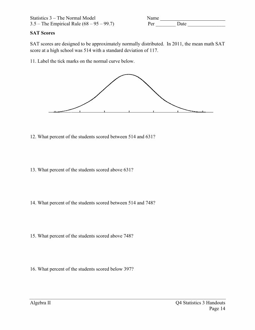
SAT Scores

SAT scores are designed to be approximately normally distributed. In 2011, the mean math SAT score at a high school was 514 with a standard deviation of 117.

11. Label the tick marks on the normal curve below.

12. What percent of the students scored between 514 and 631?

13. What percent of the students scored above 631?

14. What percent of the students scored between 514 and 748?

15. What percent of the students scored above 748?

16. What percent of the students scored below 397?



17. If there are 300 students who took the SAT at your school, approximately how many of them

scored between 514 and 631?

18. If there are 300 students who took the SAT at your school, approximately how many of them scored above 748?

Human Gestation (Length of Pregnancy)

The average length of a human pregnancy is 280 days with a standard deviation of 9 days.

19. What is the probability (percent chance) that a baby will be born between 280 and 289 days?

20. What is the probability (percent chance) that a baby will be born between 262 and 289 days?

21. What is the probability that a pregnancy will last more than 298 days?

22. If your aunt’s due date is on March 17, what is the probability that her baby will be born before March 8?

Statistics 3 – The Normal Model Name __________________________ 3.6 – Homework 2 Per ________ Date _______________


The heights of girls in an Algebra 2 class are approximately normally distributed. One particular class has an average (mean) height of 62.8 inches and standard deviation of 2.2 inches.

1. Label the tick marks on the below histogram

2. Approximately what percent of the students are taller than 62.8 inches?

3. Approximately what percent of the students are between 58.4 and 67.2 inches?

4. Approximately what percent of the students shorter than 65 inches?

5. Approximately what percent of the students are between 62.8 and 67.2 inches?

6. Approximately what percent of the students are below 58.4 inches?

7. If your class has 15 girls and their heights are similar to the ones sampled above, approximately how many of your female classmates are taller than 65 inches?

Statistics 3 – The Normal Model Name _________________________ 3.7 – Exit Pass Per ________ Date _____________


Recently, a collection of Algebra 2 students had their heart rates measured when they entered the classroom. The questions below will analyze this data.

1. The histogram above shows the heart rates of these Algebra 2 students. Describe its shape.

2. Assume that the heart rate data is approximately normally distributed with an average rate of 71 beats per minute and a standard deviation of 11. a. Label the tick marks in the histogram below using the mean and standard deviation.

b. How many standard deviations from the mean is a student with a heart rate of 82 beats per minute (bpm)?

c. Approximately what percent of the students had heart rates between 71 and 93 bpm?

d. If the class had 103 students, approximately how many had heart rates less than 60 bpm?

statistics 3 – the normal model name - edl€¦ · statistics 3 – the normal model name ... •...

Documents