statisticalanalysis of harmony and melody in rock...

Journal of New Music Research, 2013Vol. 42, No. 3, 187–204, http://dx.doi.org/10.1080/09298215.2013.788039

Statistical Analysis of Harmony and Melody in Rock Music

David Temperley1 and Trevor de Clercq2

1Eastman School of Music, University of Rochester, USA; 2Ithaca College, USA

AbstractWe present a corpus of harmonic analyses and melodic tran-scriptions of rock songs. After explaining the creation andnotation of the corpus, we present results of some explorationsof the corpus data. We begin by considering the overall dis-tribution of scale-degrees in rock. We then address the issueof key-finding: how the key of a rock song can be identifiedfrom harmonic and melodic information. Considering boththe distribution of melodic scale-degrees and the distributionof chords (roots), as well as the metrical placement of chords,leads to good key-finding performance. Finally, we discusshow songs within the corpus might be categorized with regardto their pitch organization. Statistical categorization methodspoint to a clustering of songs that resembles the major/minordistinction in common-practice music, though with some im-portant differences.

1. IntroductionIn recent years, corpus methods have assumed an increasinglyimportant role in musical scholarship. Corpus research—thatis, the statistical analysis of large bodies of naturally-occurringmusical data—provides a basis for the quantitative evalu-ation of claims about musical structure, and may also re-veal hitherto unsuspected patterns and regularities. In somecases, the information needed for a corpus analysis can be ex-tracted in a relatively objective way; examples of this includemelodic intervals and rhythmic durations in notated music(von Hippel & Huron, 2000; Patel & Daniele, 2003). In othercases, a certain degree of interpretation and subjectivity isinvolved. Harmonic structure (chords and keys) is a case ofthe latter kind; for example, expert musicians may not alwaysagree on whether something is a true ‘harmony’ or merely anornamental event. In non-notated music, even the pitches andrhythms of a melody can be open to interpretation. The useof multiple human annotators can be advantageous in thesesituations, so that the idiosyncrasies of any one individual do

Correspondence: David Temperley Eastman School of Music, 26 Gibbs St., Rochester, NY 14604, USA. E-mail: [email protected]

not overly affect the results; the level of agreement betweenannotators can also be measured, giving some indication ofthe amount of subjectivity involved.

The focus of the current study is on rock music. While rockhas been the subject of considerable theoretical discussion(Moore, 2001; Stephenson, 2002; Everett, 2009), there is littleconsensus on even the most basic issues, such as the normativeharmonic progressions of the style, the role of modes andother scale structures, and the distinction between major andminor keys. We believe that statistical analysis can inform thediscussion of these issues in useful ways, and can thereforecontribute to the development of a more solid theoretical foun-dation for rock. As with any kind of music, the understandingand interpretation of specific rock songs requires knowledgeof the norms and conventions of the style; corpus research canhelp us to gain a better understanding of these norms.

The manual annotation of harmonic and other musical in-formation also serves another important purpose: to providetraining data for automatic music processing systems. Suchsystems have recently been developed for a variety of practi-cal tasks, such as query-matching (Dannenberg et al., 2007),stylistic classification (Aucouturier & Pachet, 2003), and thelabelling of emotional content (van de Laar, 2006). Such mod-els usually employ statistical approaches, and therefore re-quire (or at least could benefit from) statistical knowledgeabout the relevant musical idiom. For example, an automatedharmonic analysis system (whether designed for symbolic oraudio input) may require knowledge about the prior prob-abilities of harmonic patterns and the likelihood of pitchesgiven harmonies. Manually-annotated data provides a way ofsetting these parameters. Machine-learning methods such asexpectation maximization may also be used, but even thesemethods typically require a hand-annotated ‘ground truth’dataset to use as a starting point.

In this paper we present a corpus of harmonic analysesand melodic transcriptions of 200 rock songs. (An earlierversion of the harmonic portion of the corpus was presented inde Clercq and Temperley (2011).) The entire corpus is

© 2013 Taylor & Francis This version has been corrected. Please see Erratum (http://dx.doi.org/10.1080/09298215.2013.839525)

Dow

nloa

ded

by [U

nive

rsity

of R

oche

ster]

at 1

2:49

20

Dec

embe

r 201

3

188 David Temperley and Trevor de Clercq

publicly available at www.theory.esm.rochester.edu/rock_corpus. We discuss our procedure for creating the corpus andexplain its format. We then present results of some explo-rations of the corpus data. We begin by considering the overalldistribution of scale-degrees in rock, comparing this to thedistribution found in common-practice music. We then discussthe issue of key-finding: how the key of a rock song can beidentified from harmonic and melodic information. Finally,we discuss how songs within the corpus might be categorizedwith regard to their pitch organization; an important questionhere is the validity of the ‘major/minor’ dichotomy in rock.

Several other corpora of popular music have been compiledby other researchers, although each of these datasets differsfrom our own in important ways. The Million-Song Dataset(Bertin-Mahieux, Ellis, Whitman, & Lamere, 2011) stands asprobably the largest corpus of popular music in existence,but only audio features—not symbolic harmonic and pitchinformation—are encoded. Datasets more similar to ours havebeen created by two groups: (1) The Center for Digital Music(CDM) at the University of London (Mauch et al., 2009),which has created corpora of songs by the Beatles, Queen, andCarole King; and (2) The McGill University Billboard Project(Burgoyne, Wild, & Fujinaga, 2011), which has compiled acorpus of songs selected from the Billboard charts spanning1958 through 1991. Both of these projects provide manually-encoded annotations of rock songs, although the data in thesecorpora is limited primarily to harmonic and timing informa-tion. Like these corpora, our corpus contains harmonic andtiming information, but it represents melodic information aswell; to our knowledge, it is the first popular music corpus todo so.

2. The corpus2.1 The Rolling Stone 500 list

The songs in our corpus are taken from Rolling Stone maga-zine’s list of the 500 Greatest Songs of All Time (2004). Thislist was created from a poll of 172 ‘rock stars and leading au-thorities’who were asked to select ‘songs from the rock’n’rollera’. The top 20 songs from the list are shown in Table 1.As we have discussed elsewhere (de Clercq & Temperley,2011), ‘rock’ is an imprecise term, sometimes used in quite aspecific sense and sometimes more broadly; the Rolling Stonelist reflects a fairly broad construal of rock, as it includes awide range of late twentieth-century popular styles such aslate 1950s rock’n’roll, Motown, soul, 1970s punk, and 1990salternative rock. Whether the songs on the list are actually thegreatest rock songs is not important for our purposes (andin any case is a matter of opinion). The list is somewhatbiased towards the early decades of rock; 206 of the songs arefrom the 1960s alone. To give our corpus more chronologicalbalance, we included the 20 highest-ranked songs on the listfrom each decade from the 1950s through the 1990s (the listonly contains four songs from 2000 or later, which we didnot include). One song, Public Enemy’s ‘Bring the Noise’,

was excluded because it was judged to contain no harmonyor melody, leaving 99 songs. We then added the 101 highest-ranked songs on the list that were not in this 99-song set,creating a set of 200 songs. It was not possible to balance thelarger set chronologically, as the entire 500-song list containsonly 22 songs from the 1990s.

2.2 The harmonic analyses

At the most basic level, our harmonic analyses consist ofRoman numerals with barlines; Figure 1(a) shows a sampleanalysis of the chorus of the Ronettes’‘Be My Baby’. (Verticalbars indicate barlines; a bar containing no symbols is assumedto continue the previous chord.) Most songs contain a largeamount of repetition, so we devised a notational system thatallows repeated patterns and sections to be represented in anefficient manner. A complete harmonic analysis using our no-tational system is shown in Figure 1(b). The analysis consistsof a series of definitions, similar to the ‘rewrite rules’ used intheoretical syntax, in which a symbol on the left is defined as(i.e. expands to) a series of other symbols on the right. Thesystem is recursive: a symbol that is defined in one expres-sion can be used in the definition of a higher-level symbol.The right-hand side of an expression is some combinationof non-terminal symbols (preceded by $), which are definedelsewhere, and terminal symbols, which are actual chords.(An ‘R’ indicates a segment with no harmony.) For example,the symbol VP (standing for ‘verse progression’) is definedas a four-measure chord progression; VP then appears in thedefinition of the higher-level unit Vr (standing for ‘verse’),which in turn appears in the definition of S (‘song’). The ‘top-level’ symbol of a song is always S; expanding the definitionof S recursively leads to a complete chord progression for thesong.

The notation of harmonies follows common conventions.All chords are built on degrees of the major scale unlessindicated by a preceding b or #; upper-case Roman numeralsindicate major triads and lower-case Roman numerals indicateminor triads. Arabic numbers are used to indicate inversionsand extensions (e.g. 6 represents first-inversion and 7 rep-resents an added seventh), and slashes are used to indicateapplied chords, e.g. V/ii means V of ii. The symbol ‘[E]’ inFigure 1(b) indicates the key. Key symbols indicate only atonal centre, without any distinction between major and minorkeys (we return to this issue below). Key symbols may alsobe inserted in the middle of an analysis, indicating a change ofkey. The time signature may also be indicated (e.g. ‘[3/4]’); if itis not, 4/4 is assumed. See de Clercq and Temperley (2011) fora more complete description of the harmonic notation system.

Given a harmonic analysis in the format just described, acustom-written computer program expands it into a ‘chordlist’, as shown in Figure 2. The first column indicates theonset time of the chord in relation to the original recording;the second column shows the time in relation to bars. (Thedownbeat of the first bar is 0.0, the midpoint of that bar is 0.5,the downbeat of the second bar is 1.0, and so on; we call this

Dow

nloa

ded

by [U

nive

rsity

of R

oche

ster]

at 1

2:49

20

Dec

embe

r 201

3

Statistical Analysis of Harmony and Melody in Rock Music 189

Table 1. The top 20 songs on the Rolling Stone list of the ‘500 Greatest Songs of All Time’.

Rank Title Artist Year

1 Like a Rolling Stone Bob Dylan 19652 Satisfaction The Rolling Stones 19653 Imagine John Lennon 19714 What’s Going On Marvin Gaye 19715 Respect Aretha Franklin 19676 Good Vibrations The Beach Boys 19667 Johnny B. Goode Chuck Berry 19588 Hey Jude The Beatles 19689 Smells Like Teen Spirit Nirvana 199110 What’d I Say Ray Charles 195911 My Generation The Who 196512 A Change Is Gonna Come Sam Cooke 196413 Yesterday The Beatles 196514 Blowin’ in the Wind Bob Dylan 196315 London Calling The Clash 198016 I Want to Hold Your Hand The Beatles 196317 Purple Haze The Jimi Hendrix Experience 196718 Maybellene Chuck Berry 195519 Hound Dog Elvis Presley 195620 Let It Be The Beatles 1970

Fig. 1. (a) A harmonic analysis of the chorus of the Ronettes’ ‘Be MyBaby’. (b) DT’s harmonic analysis of the Ronettes’ ‘Be My Baby’.

Fig. 2. Chord list for the first verse of ‘Be My Baby’, generated fromthe analysis in Figure 1(b). (The first two bars have no harmony, thusthe first chord starts at time 2.0.)

‘metrical time’.) The third column is the harmonic symbolexactly as shown in the analysis; the fourth column is thechromatic relative root, that is, the root in relation to the key(I=0, bII=1, II=2, and so on); the fifth column is the diatonicrelative root (I=1, bII=2, II=2, etc.); the sixth column showsthe key, in integer notation (C=0), and the final column showsthe absolute root (C=0).

Each of us (DT and TdC) did harmonic analyses of all200 songs. We analysed them entirely by ear, not consulting

lead sheets or other sources. We resolved certain differencesbetween our analyses, such as barline placement and timesignatures. (In most cases, the meter of a rock song is madeclear by the drum pattern, given the convention that snarehits occur on the second and fourth beats of the measure;some cases are not so clear-cut, however, especially songsin triple and compound meters.) When we found errors inthe harmonic analyses, we corrected them, but we did notresolve differences that reflected genuine disagreements aboutharmony or key.After correcting errors, the level of agreementbetween our analyses was 93.3% (meaning that 93.3% of thetime, our analyses were in agreement on both the chromaticrelative root and the key). Inspection of the differences showedthat they arose for a variety of reasons. In some cases, weassigned different roots to a chord, or disagreed as to whethera segment was an independent harmony or contained withinanother harmony; in other cases, we differed in our judgmentsof key. (See de Clercq and Temperley (2011) for further dis-cussion and examples.) While it would clearly be desirable tohave more than two analyses for each song, the high level ofagreement between our analyses suggests that the amount ofsubjectivity involved is fairly limited.

2.3 The melodic transcriptions

Many interesting questions about rock require informationabout melody as well as harmony. To investigate the melodicaspects of rock, we first needed to devise a notational systemfor transcribing rock melodies. Figure 3 shows TdC’s melodictranscription for the first verse and chorus of ‘Be My Baby’(music notation for the first four bars is shown in Figure 4,Example A). Pitches are represented as scale-degrees in rela-tion to the key: integers indicate degrees of the major scale,while other degrees are indicated with # and b symbols (e.g.

Dow

nloa

ded

by [U

nive

rsity

of R

oche

ster]

at 1

2:49

20

Dec

embe

r 201

3


Fig. 3. TdC’s melodic transcription of the first verse and chorus ofthe Ronettes’ ‘Be My Baby’. Figure 4(a) shows music notation forthe first four bars.

‘#1’). As with our harmonic notation system, vertical barsindicate barlines; each bar is assumed to be evenly divided intounits, and a unit containing no pitch event is indicated witha dot. (Only note onset times are indicated, not note offsets.)Each scale-degree is assumed to be the closest representa-tive of that scale-degree to the previous pitch: for example‘15’ indicates a move from scale-degree 1 down to scale-degree 5 rather than up, since a perfect fourth is smaller thana perfect fifth. (Tritones are assumed to be ascending.) A leapto a pitch an octave above or below the closest representa-tive can be indicated with ‘!’ or ‘"’, respectively (e.g. ‘1!5’would be an ascending perfect fifth). Keys and time signaturesare indicated in the same way as in the harmonic analyses.[OCT=4] indicates the octave of the first note, following theusual convention of note names (for example, the note name ofmiddle C is C4, thus the octave is 4). From this initial registraldesignation and the key symbol, the exact pitch of the firstnote can be determined (given the opening [E] and [OCT=4]symbols, scale-degree 1 is the note E4), and the exact pitchof each subsequent note can be determined inductively (forexample, the second note in Figure 3 is the 1 in E major closestto E4, or E4; the third note is D#4). Syllable boundaries arenot marked; a sequence of notes will be represented in thesame way whether it is under a single syllable (a melisma)or several. ‘R#4’ at the beginning indicates four bars of restbefore the vocal begins.

For the melodic transcriptions, we divided the 200-song setdescribed above into two halves: DT transcribed 100 of thesongs and TdC transcribed the other 100. Six of the songs werejudged to have no melody at all, because the vocal line waspredominantly spoken rather than sung; for these songs, nomelodic data was transcribed. (These include Jimi Hendrix’s‘Foxey Lady’, the Sex Pistols’ ‘God Save the Queen’, andseveral rap songs such as Grandmaster Flash and the FuriousFive’s ‘The Message’.) As with the harmonic analyses, wedid our melodic transcriptions by ear. We also converted thetranscriptions into MIDI files (combining them with MIDIrealizations of the harmonic analyses), which allowed us tohear them and correct obvious mistakes. At the website weprovide a script for converting an analysis such as that inFigure 3 into a ‘note list’ (similar to the chord list describedearlier), showing the absolute ontime, metrical ontime, pitch,and scale-degree of each note.

For 25 songs in the corpus, both of us transcribed the melodyof one section of the song (generally the first verse and chorus),so as to obtain an estimate of the level of agreement between

Table 2. F scores for DT’s and TdC’s melodic transcriptions withdifferent values of pitch slack (in semitones) and rhythmic slack (inbars).

Pitch

Rhythm 0 1

0 0.893 0.9201/16 0.906 0.9331/8 0.953 0.976

us. In comparing these transcriptions (and in discussing ourtranscriptions of other songs), we discovered a number ofsignificant differences of opinion. We agreed that we wantedto capture the ‘main melody’ of the song, but it is not alwaysobvious what that is. Sometimes part of a song (especially thechorus) features an alternation between two vocal parts thatseem relatively equal in prominence (usually a lead vocal anda backup group); the chorus of ‘Be My Baby’ is an exampleof this (see Figure 4, Example B). In other cases, a song mightfeature two or three voices singing in close harmony, andagain, which of these lines constitutes the main melody may bedebatable. In the first bar of Example C, Figure 4, for instance,one vocal part stays on B while the other outlines a descendingminor triad. For the 25 songs that we both transcribed, weresolved all large-scale differences of these kinds in order tofacilitate comparison; however, we did not attempt to resolvedifferences in the details of the transcriptions.

After resolving the large-scale differences described above,we compared our 25 overlapping transcriptions in the follow-ing way. Given two transcriptions T1 and T2, a note N in T2 is‘matched’ in T1 if there is a note in T1 with the same pitch andonset time as N; the proportion of notes in T2 that are matchedin T1 indicates the overall level of agreement between the twotranscriptions. We used this procedure to calculate the degreeto which DT’s transcriptions matched TdC’s, and vice versa. Ifwe arbitrarily define one set of transcriptions as ‘correct’ dataand the other as ‘model’ data, these statistics are equivalent toprecision and recall. We can combine them in the conventionalway into an F score:

F = 2/ ((1/precision) + (1/recall)) . (1)

Roughly speaking, this indicates the proportion of noteson which our transcriptions agree. (If precision and recall arevery close, as is the case here, the F score is about the same asthe mean of the precision and recall.) The F score for our 23transcriptions was 0.893. We also experimented with ‘slack’factors in both pitch and rhythm. If pitch slack is set at onesemitone, that means that a note will be considered to matchanother note if it is at the same onset time and within onesemitone. If rhythmic slack is set at 1/8 of a bar (normally one8th-note in 4/4 time), that means that a note may be matchedby another note of the same absolute pitch within 1/8 of a bar

Dow

nloa

ded

by [U

nive

rsity

of R

oche

ster]

at 1

2:49

20

Dec

embe

r 201

3


Fig. 4.

of it. F scores for various combinations of pitch and rhythmslack values are shown in Table 2.

It can be seen from Table 2 that most of the differencesbetween our analyses can be explained as small discrepanciesof pitch and/or rhythm. We inspected these differences tosee how and where they arose. In general, we found thatTdC tended to take a more ‘literal’ approach to transcription,transcribing exactly what was sung, whereas DT sought toconvey the ‘intended’ notes, allowing that these might notcorrespond exactly to the literal pitches and rhythms. A casein point is seen in the final note in Example C of Figure 4; TdCtranscribed this note as Eb4 while DT transcribed it as C4.Literally, this note is approximately Eb4. However, since thismelodic phrase is repeated many times throughout the songand generally ends with C4 (scale-degree b6), one might wellsay that this is the ‘underlying’ pitch here as well, treating theactual pitch as a quasi-spoken inflection added for emphasis.Similar differences arose in rhythm: in some cases, TdC’stranscription reflects a complex rhythm closely following theexact timing of the performance, while DT assumes a simplerunderlying rhythm. While we became aware quite early onof this slight difference in approach between us, we decidednot to try to resolve it; indeed, we felt that both ‘literal’ and‘intended’ transcriptions might be useful, depending on thepurpose for which they were being used. Another frequentsource of differences is ‘blue notes’, i.e. notes that fall ‘be-tween the cracks’ of chromatic scale-degree categories. For

example,Aretha Franklin’s ‘Respect’contains many notes thatseem ambiguous between 6 and b7, such as the third note inExample D of Figure 4. We disagreed on several of these notes,though there did not seem to be a particular bias on either ofour parts towards one degree or the other.

Despite these differences, the F score of 0.893 between ourtranscriptions showed a high enough level of agreement thatwe felt confident enough to divide the melodic transcriptiontask between us. Each of our 100 melodic transcriptions wascombined with the corresponding harmonic analysis by thesame author (DT or TdC) to create a corpus of completemelodic-harmonic encodings for 200 songs. This 200-songcollection comprises the dataset used for the statistical analy-ses described below.

3. Overall distributions of roots and scale-degreesIn the remainder of the article, we present some statisticalinvestigations of our data, and consider what they might tell usabout rock more broadly. In de Clercq and Temperley (2011),we presented a smaller version of the harmonic corpus (justthe ‘5$20’ portion) and some statistical analyses of that data.Our focus there was on the distribution of harmonies and onpatterns of harmonic motion. Here we focus on several furtherissues, incorporating the melodic data as well.

As a preliminary step, it is worth briefly examining a centralissue from our previous study in light of this larger group of

Dow

nloa

ded

by [U

nive

rsity

of R

oche

ster]

at 1

2:49

20

Dec

embe

r 201

3


Fig. 5. Root distributions in the rock corpus. For the pre-tonic and post-tonic distributions, I is excluded.

Fig. 6. Scale-degree distributions in a corpus of common-practice excerpts.

songs: the overall distribution of harmonies and scale-degrees.Figure 5 shows the distribution of chromatic relative roots, i.e.roots in relation to the local tonic, for our 200-song dataset.Note here that IV is the most common root after I, followed byV, then bVII, then VI. The graph also shows the proportionalfrequency of roots immediately before and after I (excludingI); IV is the most common chord in both ‘post-tonic’ and ‘pre-tonic’positions.This data confirms the findings in our previousstudy of the 5$20 corpus. In general, the progressions ofrock reflect a tendency towards temporal symmetry; the strongdirectional tendencies of classical harmony (e.g. the fact thatIV goes to V much more often than the reverse) are not nearlyas pronounced in rock.

We now turn to the distribution of scale-degrees, i.e. pitchesin relation to the tonic. This issue relates to the question ofwhether rock has a global ‘scale’ that favours some scale-degrees over others. Before examining our corpus data, itis interesting to consider similar data from common-practicemusic (eighteenth- and nineteenth-century Western art music).Figure 6 shows data from a corpus of 46 common-practice ex-cerpts taken from a music theory textbook (Kostka & Payne,1995; Temperley, 2001). In common-practice music, pieces(or sections of pieces) are typically identified as major or mi-nor; thus Figure 6 shows the data for major and minor excerptsseparately. As one might expect, the data from the major-key excerpts strongly reflects the major scale and the datafrom the minor-key excerpts reflects the harmonic minor scale

(containing degrees 1%2%b3%4%5%b6%7); in both profiles,tonic-triad degrees have higher values than other degrees.The figure also shows the data for major and minor excerptscombined. This reflects the union of the major and harmonicminor scales; all twelve scale-degrees are relatively frequentexcept for b2, #4, and b7. (The b7 degree is a special case; itis part of the descending melodic minor scale, but not nearlyas common in minor as 7.) The greater frequency of majordegrees over minor degrees is mainly due to the fact that thereare more major-key excerpts in the corpus.

Scale-degree distributions can be generated from our rockcorpus in two ways. First, we can generate them from theharmonic analyses, by taking each chord to denote a singleoccurrence of each pitch-class implied by the Roman numeral.For example, I of C major would contain one C, one E, andone G. Unlike the root distribution shown in Figure 5, thisdistribution incorporates information about chord quality andtype (major versus minor, triad versus seventh). However, itdoes not fully represent the true scale-degree distribution ofthe corpus. For example, the span of a chord may include manyrepetitions of a single pitch-class (or doublings in differentoctaves), or the pitch-class may not occur at all (it may onlybe implied); the span may also include notes that are not in thechord. Still, this method provides a first approximation. Thescale-degree distribution derived from our harmonic analysesis shown in Figure 7, along with the aggregate scale-degreedistribution for common-practice music.

Dow

nloa

ded

by [U

nive

rsity

of R

oche

ster]

at 1

2:49

20

Dec

embe

r 201

3


Fig. 7. Scale-degree distributions in common-practice music, rock harmony, and rock melody.

Another way to generate a scale-degree distribution is fromthe melodic transcriptions; this can be done by simply count-ing up the occurrences of each scale-degree. This melodic datais shown in Figure 7 as well. It, too, provides only a partialpicture of rock’s scale-degree distribution, since it ignoresthe accompaniment, backing vocals, and melodic instrumentallines; but the melodic information does presumably includesome non-chord tones, so in this respect it complements theharmonic scale-degree distribution.

It can be seen from Figure 7 that the three distributions—thecommon-practice distribution, the rock harmony distribution,and the rock melody distribution—are all quite similar. In allthree, the most frequent scale-degree is 1, followed by 5. Thesimilarity between the profiles is greatest in the bottom halfof the scale. All three distributions can be seen to reflect theprimacy of the major scale: 2 > b2, 3 > b3, 6 > b6, and 7 >

b7. The one exception, one that we found quite surprising, isthat in the melodic distribution—unlike the other two—b7 ismore common than 7.1 We return to this topic below.

Elsewhere, one of us (Temperley, 2001) has proposed thatrock is based on a global scale collection containing all 12scale-degrees except for b2 and #4—the ‘supermode’. Thisconcept is supported by the current data. In both the har-monic and melodic rock distributions, the two least frequentscale-degrees are b2 and #4. (This is almost true in thecommon-practice distribution as well, but b7 is just slightlyless common than #4.) This scale could be viewed as the unionof the major and natural minor scales; it also corresponds to aset of ten adjacent positions on the circle of fifths. We shouldnote, however, that in the melodic data, b6 is only slightlymore common than b2 and #4; a classification of scale-degreesinto ‘scalar’ and ‘chromatic’ might well place b6 in the lattercategory.

It might be argued that these aggregate scale-degree distri-butions tell us little, since most actual rock songs use only

1In a large corpus of European folk music, the Essen FolksongCollection (Schaffrath1995; Temperley, 2007), b7 is more commonthan 7 in minor-key melodies, though 7 is more common than b7overall.

a subset of these degrees; that is, they employ some kindof smaller scale collection within the ‘supermode’ (just asmost classical pieces use the major or minor scales rather thanthe union of them). But what exactly are these smaller scalecollections? We return to this issue in Section 5 below.

4. Key-finding4.1 Background

How do listeners determine the key of a rock song as they hearit? This is a basic and important question that can be askedabout any kind of tonal music. The problem of ‘key-finding’,as it is sometimes called, has received considerable attentionin music psychology (for a review, see Temperley, 2007b).Key-finding has practical implications as well, since manymusic-processing tasks depend on having the correct tonalframework. For example, in identifying one song as a versionor ‘cover’ of another, what is crucial is not their melodic orharmonic similarity in absolute terms—the two songs maywell be in different keys—but rather, their similarity in relationto their respective keys (Serrà, Gómez, & Herrera, 2010).

Key-finding models can be classified as to whether theyaccept audio or symbolic information as input. Clearly, audio-input models more directly reflect the situation of humanlistening. However, much of the information in an audio signalis presumably of little relevance to key—information such astimbre, percussion parts, small nuances of pitch (e.g. vibrato),and lyrics. A reasonable approach to key-finding would be toextract the information that is crucial for key identification—primarily, categorical pitch information—and then performkey-finding on that reduced representation. Indeed, someaudio key-finding models have taken exactly this approach(Cremer, 2004; Pauws, 2004). Symbolic key-finding models—such as the ones we present below—could be seen as propos-ing solutions to the second part of this process.

Most symbolic key-finding models have employed whatcould be called a distributional approach. Each key is as-sociated with an ideal distribution of pitch-classes (knownas a ‘key-profile’), and the key whose distribution most closely

Dow

nloa

ded

by [U

nive

rsity

of R

oche

ster]

at 1

2:49

20

Dec

embe

r 201

3


matches that of the piece is the preferred key; this is theessential idea behind the classic Krumhansl–Schmuckler key-finding model (Krumhansl, 1990) and several later models(Vos & Geenen, 1996; Shmulevich & Yli-Harja, 2001;Temperley, 2007b). The approach of Chew (2002) is similar,though both keys and pieces are represented by points in aspiral spatial representation. For audio key-finding, explicitpitch information is of course not available; many modelsinstead use chromas, octave-spaced frequency componentsin an audio signal corresponding to pitch-classes(Purwins, Blankertz, & Obermayer, 2000; Chai & Vercoe,2005; Gomez, 2006; Izmirili, 2007). A characteristic chromaprofile can be created for each key, and this can be matchedto the chroma content of the piece in a manner similar tokey-profile models. Some studies have addressed the moredifficult problem of deriving both harmonic structure and keysimultaneously; such models are able to take into accountthe interdependence of harmony and key (Raphael & Stod-dard, 2004; Lee & Slaney, 2007; Mauch & Dixon, 2010;Rocher, Robine, Hanna, & Oudre, 2010; Papadopoulos &Peeters, 2011).

While most of the above-mentioned studies focus onclassical music, several of them explore key estimation inpopular music. Most of these employ audio input. Lee andSlaney (2007), Mauch and Dixon (2010), and Rocher et al.(2010) test their models on the CDM Beatles corpus, men-tioned earlier; Izmirli (2007) and Papadopoulos and Peeters(2011) use both classical and popular materials. Very fewmodels have addressed the specific problem addressed here,namely, the identification of key in popular music from sym-bolic information. One study deserving mention is that ofNoland and Sandler (2006). This model estimates key fromthe transitions between chords (labelled as major or minortriads) and is tested on the CDM Beatles corpus; the modelidentifies keys with 87% accuracy.

In what follows, we explore a variety of methods foridentifying key in popular music, using our melodic tran-scriptions and harmonic analyses as input. We begin by con-sidering several models that employ pitch-class distributions;we then consider ways of estimating key directly from har-monic information. All of our models use the same basicapproach to parameter-setting and testing. The set of 200melodic-harmonic analyses described above (100 by DT, 100by TdC) was randomly split into two sets of 100; one set wasused for training (parameter-setting) and the other set was usedfor testing.

Most work on key estimation in popular music has identifiedkeys as major or minor, following the common-practice keysystem. However, we found in creating our corpus that it wasoften quite problematic to label songs as major or minor (wereturn to this issue in Section 5). Thus, we simply treat a ‘key’in rock as a single pitch-class. Another issue that arises hereconcerns modulation, that is, changes of key within a song.While most rock songs remain in a single key throughout,some songs change key: 31 of the 200 songs in our corpus con-tain at least one key change. All songs containing modulations

were placed in the training set; thus all songs used for testingcontain just one key. The identification of modulations withina song is an interesting problem, but we do not address it here.

4.2 Pitch-based key-finding

The most obvious way to apply a pitch-based key-findingstrategy given our corpus is simply to use the melodic tran-scriptions. A key-profile—a normative distribution of scale-degrees—can be generated from the melodic transcriptionsin the training set. The resulting profile is very similar to themelodic scale-degree distribution shown in Figure 7 (it is justslightly different since it is based on 100 songs rather than200). Transposing the profile produces a pitch-class profilefor each key. The key of each song in the test set can thenbe chosen by finding the pitch-class distribution of the song,which we call an input vector (following Krumhansl, 1990),and choosing the key whose profile best matches the inputvector. We measure the similarity between a key-profile andan input vector using a probabilistic method proposed byTemperley (2007b). If all keys are equal in prior probability:

argmaxkey P(key|song) = argmaxkey P(IV |key) (2)

= argmaxkey log P(IV |key)

= argmaxkey

!

pc

IV (pc) log KPkey(pc), (3)

where IV is an input vector, KP is a key-profile, pcs are pitchclasses, IV (pc) is the input-vector value for a pc, and KP(pc)is the key-profile value for a pc. The final expression abovecan also be viewed as the (negative) cross-entropy between thekey-profile and the input vector.Asimilar matching procedureis used in all the models presented below.

We call this Model 1; it is essentially equivalent to the mono-phonic key-finding model proposed in Temperley (2007b).Table 3 shows the model’s performance on the 100-song testset. We also reasoned that it might help to weight each noteaccording to its duration, as in Krumhansl’s (1990) model.This cannot easily be done in our data set, since only noteonsets are indicated, not offsets. In general, however, theoffset of a melodic note approximately coincides with the nextnote onset (it could not be later than the next onset, giventhe limitations of the human voice), unless the time intervalbetween the two onsets is very long; in the latter case, thereis often a rest between the two notes (this frequently happensat phrase boundaries, for example). Thus we define the lengthof a note as its inter-onset interval (the time interval betweenits onset and the next, in metrical time) or one bar, whicheveris less. With notes thus weighted for duration, key-profilesand input vectors can be constructed as they were in Model 1.This is Model 2; as shown in Table 3, it performs somewhatbetter than Model 1. Since long notes tend to occur at the endsof phrases, the superior performance of Model 2 may in partbe due to the fact that it is giving extra weight to notes inphrase-final positions.

Dow

nloa

ded

by [U

nive

rsity

of R

oche

ster]

at 1

2:49

20

Dec

embe

r 201

3


Table 3. Key-finding models.

Number of % correctModel Description parameters

1 Melodic scale-degree (SD) distribution 12 762 Melodic SD distribution, weighted for duration 12 823 Harmonic SD distribution, weighted for duration 12 784 Weighted mel. SD dist. + weighted harm. SD dist. 24 865 Root distribution 12 776 Root dist. weighted for duration 12 867 Root dist. distinguishing metrically strong vs. weak 24 898 Root dist. weighted for duration, distinguishing 24 91

strong vs. weak9 Root dist. weighted for duration, distinguishing 36 97

strong vs. weak, + weighted melodic SD dist.

Models 1 and 2 only use melodic information, and thereforeconsider only part of the pitch-class content of the piece.Another approach to pitch-based key-finding is to use a har-monic analysis to generate an approximate distribution ofpitch-classes—taking each chord to imply one instance ofeach pitch-class it contains, as was done in Section 3 above(the resulting profile is very similar to the rock harmony dis-tribution in Figure 7). As with our melodic models, we foundthat weighting each event by its length improved performance;in this case, the length of a note is defined by the length ofthe chord that contains it, which is explicitly indicated in ourharmonic analyses. Key-profiles and input vectors can then begenerated in the usual way. The results of this model (Model 3)are shown in Table 3; the model performs slightly less wellthan the duration-weighted melodic model.

As noted earlier, the melodic and harmonic scale-degreedistributions are in a sense complementary. The harmonicdistribution includes accompaniment parts and instrumentalsections, but excludes non-harmonic notes; the melodic dis-tribution includes such notes but considers only the melody. Alogical next step, therefore, is to combine the two distributions,creating a profile with 24 values. This model, Model 4, per-forms slightly better than Model 2, which considers melodicinformation alone. We earlier noted some differences betweenthe harmonic and melodic key-profiles, notably the greaterfrequency of b7 in the melodic profile; recognizing this dis-tinction appears to have a small benefit for key-finding.

4.3 Harmony-based key-finding

Even the best of our pitch-based key-finding models leavesconsiderable room for improvement. An alternative approachis to estimate key directly from harmonic information.Noland and Sandler (2006) employ this strategy, with goodresults; their model looks at transitions between chords—theassumption being that important information about key mightlie in the temporal ordering of chords. We have found, how-ever, that the strong ordering constraints of classical harmonyare much less present in rock: for example, the frequencyof the IV chord does not seem to vary greatly depending on

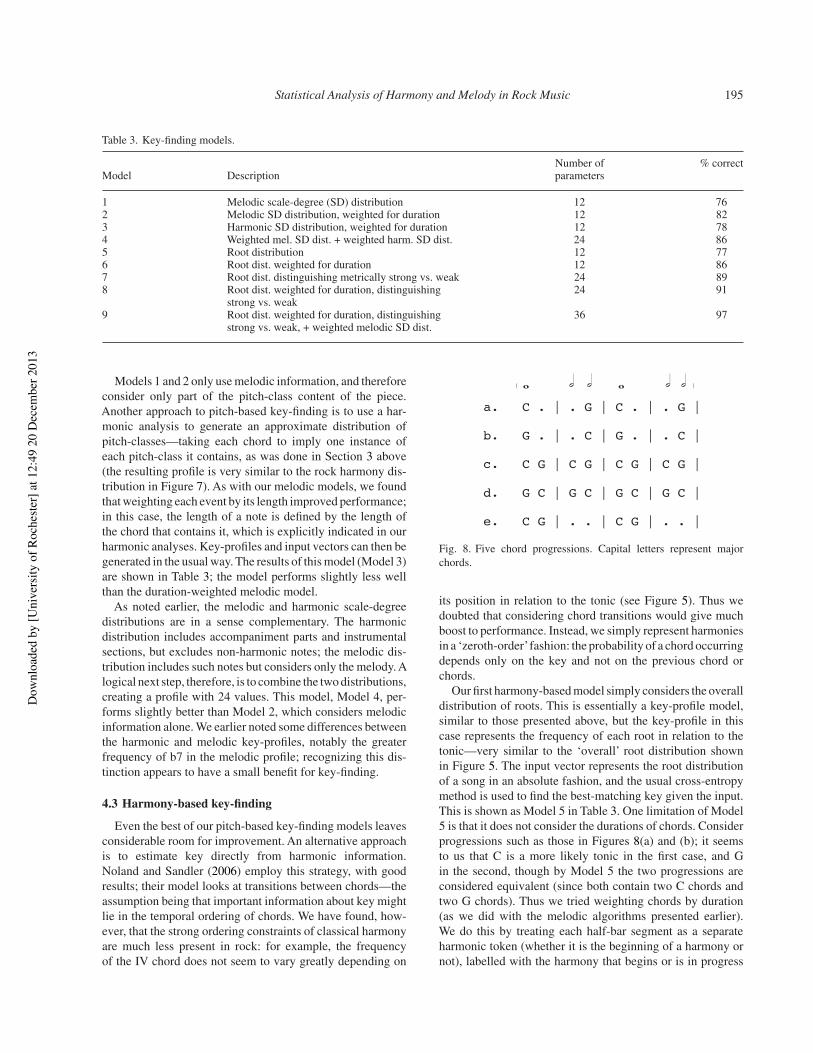
Fig. 8. Five chord progressions. Capital letters represent majorchords.

its position in relation to the tonic (see Figure 5). Thus wedoubted that considering chord transitions would give muchboost to performance. Instead, we simply represent harmoniesin a ‘zeroth-order’fashion: the probability of a chord occurringdepends only on the key and not on the previous chord orchords.

Our first harmony-based model simply considers the overalldistribution of roots. This is essentially a key-profile model,similar to those presented above, but the key-profile in thiscase represents the frequency of each root in relation to thetonic—very similar to the ‘overall’ root distribution shownin Figure 5. The input vector represents the root distributionof a song in an absolute fashion, and the usual cross-entropymethod is used to find the best-matching key given the input.This is shown as Model 5 in Table 3. One limitation of Model5 is that it does not consider the durations of chords. Considerprogressions such as those in Figures 8(a) and (b); it seemsto us that C is a more likely tonic in the first case, and Gin the second, though by Model 5 the two progressions areconsidered equivalent (since both contain two C chords andtwo G chords). Thus we tried weighting chords by duration(as we did with the melodic algorithms presented earlier).We do this by treating each half-bar segment as a separateharmonic token (whether it is the beginning of a harmony ornot), labelled with the harmony that begins or is in progress

Dow

nloa

ded

by [U

nive

rsity

of R

oche

ster]

at 1

2:49

20

Dec

embe

r 201

3


Fig. 9. Key-profiles for metrically strong and weak harmonies.

at the beginning of the segment; the key-profile and inputvector represent counts of these tokens. (About 3% of chordsin our analyses do not span any half-bar point; these areeffectively ignored.) Thus a harmony that extends over severalhalf-bar segments will carry more weight. The resulting modelis shown in Table 3 as Model 6.

We suggested that the preference for C over G as tonalcentre in Figure 8(a) might be due to the greater duration of Charmonically.Another factor may be at work as well, however.Some authors have suggested that the metrical placement ofharmonies plays an important role in key-finding in rock: thereis a strong tendency to favour a key whose tonic chord appearsat metrically strong positions (Temperley, 2001; Stephenson,2002). This would have the desired result in Figures 8(a) and(b) (favouring C in the first case and G in the second) but itwould also distinguish Figures 8(c) and (d) (which Model 6would not), favouring C in the first case and G in the second,which we believe is correct. Model 7 is similar to Model 5, inthat it counts each chord just once, but it maintains one key-profile for chords beginning at metrically strong positions andanother profile for other chords, and also distinguishes thesecases in the input vector. We experimented with different waysof defining ‘metrically strong’; the most effective methodwas to define a strong position as the downbeat of an odd-numbered bar (excluding any partial bar or ‘upbeat’ at thebeginning of the song). The profiles for weak and strongharmonies are shown in Figure 9; it can be seen that, indeed,the main difference is the much higher frequency of tonic in themetrically strong profile. (The data in Figure 9 also indirectlyconfirm our assumption that, in general, odd-numbered barsin rock songs are metrically strong. Many rock songs arecomposed entirely of four-bar units in which the first and thirdbars of each unit feel metrically stronger than the second andfourth. There are certainly exceptions, however; a number ofsongs in our corpus contain irregular phrases, so that the corre-spondence between odd-numbered bars and strong downbeatsbreaks down. No doubt a more accurate labelling of metricallystrong bars would improve the performance of Model 7, butwe will not attempt that here.)

Model 7 yields a slight improvement over previous models,but further improvement is still possible. Model 7 considersonly the starting position of chords, not their length; therefore

the two progressions in Figures 8(c) and (e) are treated asequivalent, since in both cases, all the C chords are strongand all the G chords are weak. But it seems to us that thegreater duration of G in Figure 8(e) gives a certain advantageto the corresponding key. Model 8 combines Models 6 and 7:we count each half-bar separately, but use different distribu-tions for ‘strong’ half-bars (those starting on odd-numbereddownbeats) and ‘weak’ ones. The result on the test set is 91%correct, our best result so far.

As a final step, we experimented with combining the harmony-based approach with the pitch-based approach presented ear-lier. Our harmonically-generated pitch profiles contain muchof the same information as the root-based profiles, so it seemssomewhat redundant to use them both. Instead, we combinedthe melodic pitch profiles with the root profiles. Specifically,we combined the weighted melodic profile (Model 2) with thedurationally-weighted and metrically-differentiated root pro-file (Model 8), yielding a profile with 36 values. The resultingmodel, Model 9, identifies the correct key on 97 of the 100songs.

The accuracy of Model 9 may be close to the maximum pos-sible, given that there is not 100% agreement on key labellingeven among human annotators. (With regard to key, our analy-ses were in agreement with each other 98.2% of the time.) Weinspected the three songs on which Model 9 was incorrect, totry to understand the reason for its errors. On Prince’s ‘WhenDoves Cry’, the tonal centre is A but the model chose G. Muchof the song consists of the progression ‘Am | G | G |Am |’; thusboth G and Am occur at both hypermetrically strong and weakpositions. Perceptually, what favoursAover G as a tonal centreseems to be the fact that Am occurs on the first measure ofeach group of four, while G occurs on the third; incorporatingthis distinction into our model might improve performance.Another song, ‘California Love’, consists almost entirely of arepeated one-measure progression ‘F G . . |’; G is the true tonic,but F is favoured by the model due to its metrical placement,outweighing the strong support for G in the melody. Finally,in the Clash’s ‘London Calling’, the true tonal centre is E, butthe unusually prominent use of the bII chord (F major) causesG to be favoured. The verse of this song is, arguably, tonallyambiguous; what favours E over G seems to be the strongharmonic and melodic move to E at the end of the chorus.

Dow

nloa

ded

by [U

nive

rsity

of R

oche

ster]

at 1

2:49

20

Dec

embe

r 201

3


These errors suggest various possible ways of improving themodel, but there does not appear to be any single ‘silver bullet’that would greatly enhance performance.

The success of our models, and in particular Model 9, pointsto several important conclusions about key-finding in rock.First, both the distribution of roots and the distribution ofmelodic pitch-classes contain useful information about key,and especially good results are obtained when these sources ofinformation are combined. Second, the conjecture ofTemperley(2001) and Stephenson (2002) regarding the metrical place-ment of harmonies is confirmed: key-finding from root infor-mation is considerably improved when the metrical strength ofharmonies is taken into account. Finally, we see little evidencethat considering chord transitions is necessary for key-finding;it appears possible to achieve nearly perfect performance bytreating chords in a ‘zeroth-order’ fashion.

It is difficult to evaluate this model in relation to the othermodels of key-finding surveyed earlier. To compare symbolickey-finding models to audio ones hardly seems fair, given thegreater difficulty of the latter task. The only model designedfor symbolic key-finding in popular music, to our knowledge,is that of Noland and Sandler (2006), which achieved 87%on a corpus of Beatles songs (performance rose to 91% whenthe model was trained on each song). Their task was some-what more difficult than ours, as their model was required tocorrectly identify keys as major or minor. On the other hand,our models are considerably simpler than theirs. By their owndescription, Noland and Sandler’s model requires 2401$24 =57,624 parameters (though it seems that this could be reducedby a factor of 12 by assuming the same parameters acrossall major keys and all minor keys). By contrast, our best-performing model requires just 36 parameters. In general,our experiments suggest that key-finding can be done quiteeffectively—at least from symbolic data—with a fairly smallnumber of parameters.

5. Clustering songs by scale-degree distributionAnother purpose for which our corpus might be used is thecategorization of songs based on musical content. While manystudies have used statistical methods for the classificationof popular music (for a review, see Aucouturier and Pachet(2003)), none, to our knowledge, have used symbolic rep-resentations as input. In addition, most previous studies ofmusic classification have had practical purposes in mind (suchas predicting consumer tastes). By contrast, the current studyis undertaken more in the spirit of basic research: we wishto explore the extent to which rock songs fall into naturalcategories or clusters by virtue of their harmonic or melodiccontent, in the hope that this will give us a better understandingof the style.

An issue of particular interest is the validity of the distinc-tion between major and minor keys. Corpora of popular musicsuch as the CDM Beatles corpus (Mauch et al., 2009) andthe Million-Song Dataset (Bertin-Mahieux et al., 2011) labelsongs as major or minor, and key-finding models that use these

corpora for testing have generally adopted this assumption aswell. However, a number of theorists have challenged the va-lidity of the major/minor dichotomy for rock (Covach, 1997;Stephenson, 2002) or have proposed quite different systemsfor categorizing rock songs by their pitch content (Moore,1992; Everett, 2004). As Moore has discussed, some songsare modal in construction, meaning that they use a diatonicscale but with the tonic at varying positions in the scale. Forexample, the Beatles’ ‘Let it Be’, the Beatles’ ‘PaperbackWriter’, and REM’s ‘Losing My Religion’ all use the notesof the C major scale; but the first of these three songs has atonal centre of C (major or Ionian mode), the second has a tonalcentre of G (Mixolydian mode), and the third has a tonal centreof A (natural minor or Aeolian mode). Pentatonic scales alsoplay a prominent role in rock (Temperley, 2007a). Still othersongs employ pitch collections that are neither diatonic norpentatonic: for example, the chord progression of the chorusof the Rolling Stones’ ‘Jumping Jack Flash’, Db major/Abmajor/Eb major/Bb major, does not fit into any diatonic modeor scale. Similarly, the verse of the Beatles’ ‘Can’t Buy meLove’ features the lowered (minor) version of scale-degree3 in the melody over a major tonic triad in the accompani-ment, thus resisting classification into any conventional scale.Some authors have explained such phenomena in terms of‘blues scales’, or blues-influenced inflections of diatonic orpentatonic scales (van der Merwe, 1989; Stephenson, 2002;Wagner, 2003).2

In short, the status of the major/minor dichotomy with re-gard to rock is far from a settled issue. The statistical datapresented earlier in Section 3 could be seen as providingsome insight in this regard. On the one hand, the fact that thescale-degree distribution of rock (both harmonic and melodic)is quite similar to that of classical music might suggest thepresence of some kind of major/minor organization. On theother hand, important differences also exist: in particular, b7is much more common than 7 overall in our melodic corpus,whereas the opposite situation is found with both major andminor keys in classical music. To better explore this topic,the following section presents ways of using our corpus todetermine whether the major/minor distinction is applicableto rock, and if not, what other natural categories might exist.

5.1 The binary vector approach

To explore the presence of major and minor scales in rock,as well as other scale formations, we need some way of mea-suring the adherence of a song to a particular scale. As a firststep, we might define ‘adherence to a scale’ in a strict sense,meaning that all degrees of the scale must be used and noothers. To this end, we can represent the scale-degree contentof each song as a binary 12-valued vector, with ‘1’ in each

2A number of authors have discussed the ‘blues scale’, but it is rarelydefined in a precise way. Van der Merwe (1989) defines it as the majorscale with added flat versions of the 3rd, 5th, 6th, and 7th degrees;thus it includes all twelve chromatic degrees except b2.

Dow

nloa

ded

by [U

nive

rsity

of R

oche

ster]

at 1

2:49

20

Dec

embe

r 201

3


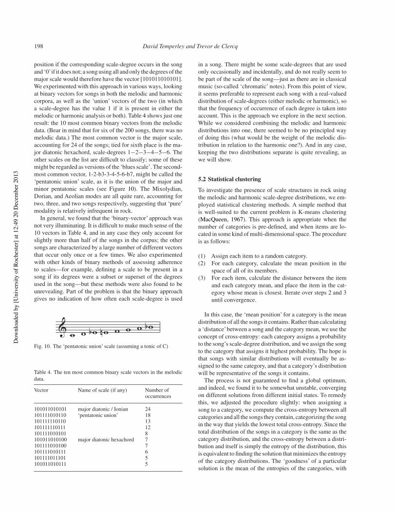
position if the corresponding scale-degree occurs in the songand ‘0’if it does not; a song using all and only the degrees of themajor scale would therefore have the vector [101011010101].We experimented with this approach in various ways, lookingat binary vectors for songs in both the melodic and harmoniccorpora, as well as the ‘union’ vectors of the two (in whicha scale-degree has the value 1 if it is present in either themelodic or harmonic analysis or both). Table 4 shows just oneresult: the 10 most common binary vectors from the melodicdata. (Bear in mind that for six of the 200 songs, there was nomelodic data.) The most common vector is the major scale,accounting for 24 of the songs; tied for sixth place is the ma-jor diatonic hexachord, scale-degrees 1%2%3%4%5%6. Theother scales on the list are difficult to classify; some of thesemight be regarded as versions of the ‘blues scale’. The second-most common vector, 1-2-b3-3-4-5-6-b7, might be called the‘pentatonic union’ scale, as it is the union of the major andminor pentatonic scales (see Figure 10). The Mixolydian,Dorian, and Aeolian modes are all quite rare, accounting fortwo, three, and two songs respectively, suggesting that ‘pure’modality is relatively infrequent in rock.

In general, we found that the ‘binary-vector’ approach wasnot very illuminating. It is difficult to make much sense of the10 vectors in Table 4, and in any case they only account forslightly more than half of the songs in the corpus; the othersongs are characterized by a large number of different vectorsthat occur only once or a few times. We also experimentedwith other kinds of binary methods of assessing adherenceto scales—for example, defining a scale to be present in asong if its degrees were a subset or superset of the degreesused in the song—but these methods were also found to beunrevealing. Part of the problem is that the binary approachgives no indication of how often each scale-degree is used

Fig. 10. The ‘pentatonic union’ scale (assuming a tonic of C)

Table 4. The ten most common binary scale vectors in the melodicdata.

Vector Name of scale (if any) Number ofoccurrences

101011010101 major diatonic / Ionian 24101111010110 ‘pentatonic union’ 18101111110110 13101111110111 12101111010101 8101011010100 major diatonic hexachord 7101111010100 7101111010111 6101111011101 5101011010111 5

in a song. There might be some scale-degrees that are usedonly occasionally and incidentally, and do not really seem tobe part of the scale of the song—just as there are in classicalmusic (so-called ‘chromatic’ notes). From this point of view,it seems preferable to represent each song with a real-valueddistribution of scale-degrees (either melodic or harmonic), sothat the frequency of occurrence of each degree is taken intoaccount. This is the approach we explore in the next section.While we considered combining the melodic and harmonicdistributions into one, there seemed to be no principled wayof doing this (what would be the weight of the melodic dis-tribution in relation to the harmonic one?). And in any case,keeping the two distributions separate is quite revealing, aswe will show.

5.2 Statistical clustering

To investigate the presence of scale structures in rock usingthe melodic and harmonic scale-degree distributions, we em-ployed statistical clustering methods. A simple method thatis well-suited to the current problem is K-means clustering(MacQueen, 1967). This approach is appropriate when thenumber of categories is pre-defined, and when items are lo-cated in some kind of multi-dimensional space. The procedureis as follows:

(1) Assign each item to a random category.(2) For each category, calculate the mean position in the

space of all of its members.(3) For each item, calculate the distance between the item

and each category mean, and place the item in the cat-egory whose mean is closest. Iterate over steps 2 and 3until convergence.

In this case, the ‘mean position’ for a category is the meandistribution of all the songs it contains. Rather than calculatinga ‘distance’between a song and the category mean, we use theconcept of cross-entropy: each category assigns a probabilityto the song’s scale-degree distribution, and we assign the songto the category that assigns it highest probability. The hope isthat songs with similar distributions will eventually be as-signed to the same category, and that a category’s distributionwill be representative of the songs it contains.

The process is not guaranteed to find a global optimum,and indeed, we found it to be somewhat unstable, convergingon different solutions from different initial states. To remedythis, we adjusted the procedure slightly: when assigning asong to a category, we compute the cross-entropy between allcategories and all the songs they contain, categorizing the songin the way that yields the lowest total cross-entropy. Since thetotal distribution of the songs in a category is the same as thecategory distribution, and the cross-entropy between a distri-bution and itself is simply the entropy of the distribution, thisis equivalent to finding the solution that minimizes the entropyof the category distributions. The ‘goodness’ of a particularsolution is the mean of the entropies of the categories, with

Dow

nloa

ded

by [U

nive

rsity

of R

oche

ster]

at 1

2:49

20

Dec

embe

r 201

3


Fig. 11. Profiles for the two categories (C1 and C2) revealed by the K-means analysis of the melodic data.

Fig. 12. Profiles for the two categories revealed by the K-means analysis of the harmonic data.

each category weighted by the number of songs it contains.This procedure was found to be stable; repeating the processfrom many different initial states always led to exactly thesame solution.

The two-category solution for the melodic data is shownin Figure 11; the categories are arbitrarily labelled 1 and 2.Category 1 clearly represents the major scale; the seven majordegrees have much higher values than the other five. Withinthe major scale, the five degrees of the major pentatonic scale(1%2%3%5%6) have the highest values. Category 2 is moredifficult to characterize. One could call it a kind of minordistribution, since it has a much higher value for b3 than for3. It does not, however, resemble classical minor; 6 is muchmore common than b6, and b7 is much more common than7, whereas in classical minor the reverse is true in both cases(see Figure 6). It is notable also that the value for 3 is fairlyhigh in this profile. If one were to interpret this distributionas implying a scale, the closest approximation would appearto be the 8-note scale 1%2%b3%3%4%5%6%b7; these eightdegrees have far higher values than the remaining four. This isthe ‘pentatonic union’ scale that also emerged as the second-most common binary vector in the melodic data (see Table 4and Figure 10).

The two-category solution for the harmonic data is shownin Figure 12. Here again, category 1 very strongly reflects themajor scale. Category 2 could again be described as some kind

of minor (though the value for 3 is fairly high); b7 is far morecommon than 7 (as in the melodic ‘minor’ category) but 6 andb6 are nearly equal.

Both the melodic and harmonic data give some support tothe validity of the major/minor distinction in rock. In bothcases, two strongly distinct profiles emerge: in one profile, 3dominates over b3, while in the other profile the reverse is true.In all four profiles, the three tonic-triad degrees (1%3%5 forcategory 1 profiles and 1%b3%5 for the category 2 profiles)are more common than any others, giving further support toa major/minor interpretation. It seems reasonable to refer tothese profiles as ‘major’ and ‘minor’, and we will henceforthdo so. While the major rock profiles strongly resemble clas-sical major, the minor rock profiles are quite unlike classicalminor, favouring the lowered seventh degree and the raisedsixth, and with a significant presence of 3 as well.

Table 5. The number of songs in the major and minor harmonic andmelodic categories.

Harmonic Melodic

Major Minor

Major 98 41Minor 9 46

Dow

nloa

ded

by [U

nive

rsity

of R

oche

ster]

at 1

2:49

20

Dec

embe

r 201

3


Fig. 13. The first eigenvector of the principal components analysis of the harmonic scale-degree vectors, showing the projection of eachscale-degree.

In both the melodic and harmonic classification systems,there are more songs in the major category than the minorone, though the preponderance of major songs is greater in theharmonic data. Related to this, one might ask how strongly themelodic and harmonic classification schemes are correlatedwith one another. To address this, we can label each songby both its melodic and harmonic categories; the numbersare shown in Table 5. Not surprisingly (given the similaritybetween the profiles of the two categorization systems), theyare indeed strongly correlated; 144 of the 194 songs (for whichthere is both melodic and harmonic data) are either major inboth the melodic and harmonic systems, or minor in both sys-tems. Interestingly, the vast majority of the remaining songsare minor in the melodic system and major in the harmonicone, rather than vice versa; we will call these ‘minor/major’songs (stating the melodic category first). We noted earlierthat some songs feature a minor third in the melody over amajor tonic triad (the Beatles’ ‘Can’t Buy me Love’was givenas an example); the current data suggests that this pattern israther common. Closer inspection of the results showed thatthe ‘minor/major’ category consists largely of 1950s songssuch as Elvis Presley’s ‘Hound Dog’, blues-influenced rocksongs such as the Rolling Stones’ ‘Satisfaction’, and soul hitssuch as Aretha Franklin’s ‘Respect’.

We also experimented with higher numbers of categories. Inthe melodic case, a 3-category solution (not shown here) yieldsone category very similar to the 2-category major profile.The other two categories both resemble the minor profile;they differ from each other mainly in that one has a muchhigher value for 1 and lower values for 4 and 5. (This mayreflect differences in melodic register—the part of the scalein which the melody is concentrated—rather than in the scaleitself.) In the harmonic case, the 3-category solution is quitedifferent from the 2-category one: the first category reflectsmajor mode, the second is similar to major but with b7 slightlyhigher than 7, and the third reflects Aeolian (with b3 > 3, b6> 6 and b7 > 7). In both the melodic and harmonic data,however, the 3-category system is only very slightly lowerin entropy than the 2-category one (less than 2%), thus itoffers little improvement over the 2-category solution as acharacterization of the data.

5.3 Principal component analysis

We explored one further approach to the classification of rocksongs: principal component analysis. Let us imagine eachsong’s scale-degree distribution (melodic or harmonic) as apoint in a 12-dimensional space, with each dimension repre-senting a scale-degree. Some dimensions may be correlated

with one another, meaning that when scale-degree X has a highvalue in the distribution, scale-degree Y is also likely to havea high value; other dimensions may be negatively correlated.Principal component analysis searches for such correlationsamong dimensions and creates new axes that represent them.More precisely, it tries to establish a new coordinate systemthat explains as much of the variance as possible among pointsin the space with a small number of axes, or eigenvectors.Each eigenvector is associated with an eigenvalue, indicat-ing the amount of variance it explains; an eigenvector thatexplains a large amount of variance can act as a kind ofsummary of statistical tendencies in the data. The analysiscreates as many eigenvectors as there are dimensions in theoriginal data, and outputs them in descending order accordingto how much variance they explain; the first few eigenvectors(those explaining the most variance) are generally of the mostinterest.

The data for the analysis is the melodic and harmonic scale-degree distributions for individual songs, used in the clusteringexperiment described earlier. We begin with the harmonicdata. The first eigenvector (that is, the one explaining the mostvariance) accounted for 31% of the variance. (The secondeigenvector accounted for only 19% of the variance, and wecannot find any good interpretation for it, so we will say nomore about it.) Figure 13 shows the projections of each ofthe original dimensions on the first eigenvector. It can beseen that the three most negative dimensions are 3, 6, and7, and the three most positive ones are b3, b6, and b7. Whatthis tells us is that 3, 6, and 7 form a group of scale-degreesthat are positively correlated with one another; b3, b6, and b7form another group that are positively correlated; and the twogroups are negatively correlated with one another. In short,the analysis provides another strong piece of evidence thatmajor/minor dichotomy is an important dimension of variationin rock music.

A similar analysis was performed with the melodic scale-degree distributions. In this case, the first two eigenvectorswere fairly close in explanatory power, the first one explaining25% of the variance and the second one explaining 19%.The scatterplot in Figure 14 shows the projections of eachscale-degree on to the first (horizontal) and second (verti-cal) eigenvectors. The first eigenvector appears to reflect themajor/minor spectrum, though not quite as clearly as in theharmonic data; 3, 6, and 7 are positive while b3 and b7 arenegative. (b6 is also negative, but only weakly so; this maysimply be due to its low frequency in the melodic data.) Thesecond eigenvector is not so easy to explain. We suspect thatit reflects phenomena of register. The most positive degreein the vertical direction is 5, and the most negative one is

Dow

nloa

ded

by [U

nive

rsity

of R

oche

ster]

at 1

2:49

20

Dec

embe

r 201

3


1; perhaps melodies tend to be centred on either 5 or 1, butnot both, meaning that the two degrees are somewhat nega-tively correlated. Note further that #4, 4, and b6, like 5, arestrongly positive; no doubt, when a melody is centred on 5, ittends to make frequent use of scale-degrees that are nearby inpitch height. This explanation only goes so far, however; 1 isstrongly negative, but the degrees closest to it in height—b2,2, b7, and 7—are not.

A small set of eigenvectors produced by a principal compo-nents analysis can be viewed as a reduction or simplificationof the original space; it can then be revealing to project theoriginal data vectors on to that reduced space. As an ex-ample, consider a hypothetical song whose harmonic scale-degree vector is a perfectly even distribution of the sevenmajor scale-degrees, with no other scale-degrees: i.e. the vec-tor [1/7,0,1/7,0,1/7,1/7,0,1/7,0,1/7,0,1/7]. To project this onto the eigenvector represented in Figure 13, we take the dotproduct of this vector with the eigenvector.This is proportionalto the mean of the values of the eigenvector for which thesong vector is nonzero. The location of our major (‘Ionian’)song on the axis is shown in Figure 15(a), as well as sim-ilar hypothetical songs in Mixolydian, Dorian, and Aeolianmodes; these are the four modes that are generally said to becommon in rock (Moore, 1992). It is well known that eachdiatonic mode contains a set of seven consecutive positionson the circle of fifths—sometimes known as the ‘line of fifths’(Temperley, 2001)—and that the modes themselves reflect anatural ordering on the line (see Figure 15(b)); this is exactlythe ordering that emerges from the projection in Figure 15(a).In this sense, it could be said that the line of fifths is implicit inthe eigenvector (although the projection of individual scale-degrees does not reflect the line of fifths, as seen in Figure 13).3

As noted earlier, the ‘supermode’—the set of all scale-degreescommonly used in rock music, including all twelve degreesexcept b2 and #4—also reflects a set of adjacent positionson the line. It has been proposed that an axis of fifths playsan important role in the perception of pitch and harmony(Krumhansl, 1990) and also in the emotional connotationsof melodies (Temperley & Tan, in press), suggesting that it ispart of listeners’ mental representation of tonal music. Theimplicit presence of the line of fifths in the scale-degree dis-tribution of popular music may explain how listeners are ableto internalize it from their musical experience.

3This argument does not work so well for the Lydian and Phrygianmodes; in terms of line-of-fifths ordering of scale-degrees, Lydianshould be to the left of Ionian in Figure 15(a) but is actually to itsright, and Phrygian should be to the right of Aeolian but is actuallyto its left. Because #4 and b2 are so rare, their distribution in ourcorpus may not reflect their true distribution. In addition, the currentanalysis is assuming only a single spelling of these pitches, but infact each one has two different spellings (#4 vs. b5, b2 vs. #1) whichhave different locations on the line of fifths. (For all other scale-degrees, a single spelling accounts for the vast majority of its uses.)Incorporating spelling distinctions raises many difficult practical andtheoretical issues, however, so we will not attempt it here.

Fig. 14. The first (horizontal) and second (vertical) eigenvectorsof the principal components analysis of the melodic scale-degreevectors.

Fig. 15. (a) Projection of hypothetical modal melodies on to the axisshown in Figure 13. (b) Diatonic modes on the line of fifths.

We can also project each of the individual harmonic scale-degree vectors in our corpus on to the first harmonic eigen-vector; this gives an indication of where each song lies on themajor/minor axis. While we will not explore this in detail, theaggregate results are shown in Figure 16; songs are ‘bucketed’into small ranges of 0.01. The distribution that emerges is ofinterest in two ways. First of all, it is essentially unimodal,featuring a single primary peak (there is only a very small peaktoward the right end of the distribution); this suggests that rocksongs are rather smoothly distributed along the major/minordimension rather than falling into two neat categories. It isalso noteworthy that the primary peak is far towards the left(major) end of the distribution; we are not sure what to makeof this.

The results presented here, as well as the results of the clus-ter analysis presented previously, suggest that the major/minorcontrast is an important dimension of variation in the pitchorganization of rock music. The distinctively major scale-degrees 3, 6, and 7 tend to be used together, as do the dis-tinctively minor degrees b3, b6, and b7; and the two groups ofdegrees are, to some extent at least, negatively correlated withone another. This does not mean that the major/minor systemof classical tonality can be imposed wholesale on rock; indeed,

Dow

nloa

ded

by [U

nive

rsity

of R

oche

ster]

at 1

2:49

20

Dec

embe

r 201

3


Fig. 16. Projections of the 200 harmonic scale-degree vectors on tothe first harmonic eigenvector, bucketed into ranges of 0.01. Numberson the horizontal axis indicate the centre of each bucket.

we have suggested it cannot. But some kind of major/minorspectrum is clearly operative. One might ask whether thisdimension correlates in any way to conventional generic cat-egories of rock; we suspect that it does. For example, in termsof our cluster analysis, we observe that heavy metal songs—such as Steppenwolf’s ‘Born to be Wild’, AC/DC’s ‘Backin Black’, and Metallica’s ‘Enter Sandman’—tend to be inthe minor category both melodically and harmonically, whilegenres such as early 1960s pop (the Ronettes’ ‘Be My Baby’,the Crystals’ ‘Da Doo Ron Ron’) and 1970s soft rock (EltonJohn’s ‘Your Song’) tend to be melodically and harmonicallymajor. We have already noted that the ‘minor/major’ cluster(songs that are minor melodically and major harmonically)is associated with certain stylistic categories as well. Froma practical point of view, this suggests that the major/minordimension might be a useful predictor (in combination withothers, of course) of listeners’ judgments about style.

6. Conclusions and future directionsThe statistical analyses and experiments presented in this pa-per point to several conclusions about rock. The overall scale-degree distribution of rock, both melodically and harmoni-cally, is quite similar to that of common-practice music. Inrock, as in common-practice music, all twelve degrees appearquite commonly except #4 and b2 (though b6 is borderline inthe melodic distribution). The most prominent difference isthat b7 is more common than 7 in rock melodies, whereas incommon-practice music the reverse is true. Our experiments inkey identification suggest that key-finding in rock can be donequite effectively with a purely distributional approach, usinga combination of melodic scale-degree information and rootinformation, and taking the metrical position of harmoniesinto account. Finally, our experiments with clustering andprincipal components analysis suggest that the major/minordichotomy is an important dimension of variation in rock,though it operates quite differently from that in common-practice music in several respects. In the minor mode of rock,if one can call it that, 6 is favoured over b6, and b7 over 7; asignificant proportion of songs are minor melodically but ma-

jor harmonically; and the distribution of songs between majorand minor appears to reflect more of a gradual continuum thantwo discrete categories.

One unexpected result of our analyses is the strong presenceof the ‘pentatonic union’ scale, 1%2%b3%3%4%5%6%b7, inthe melodic data. This scale is the second most common binaryvector in the melodic transcriptions; it also emerges stronglyin the ‘minor’ category of the melodic cluster analysis. More-over, in 37 of the 194 melodies, the eight degrees of the penta-tonic union scale are the most frequent of the twelve chromaticdegrees; no other scale (of comparable size) seems to rival thisexcept the major scale, whose degrees are the most frequentin 46 songs. Thus, three different statistical methods point tothe pentatonic union scale as an important tonal structure inrock. To our knowledge, this scale has not been discussedpreviously. As well as being the union of the two pentatonicscales, it has several other interesting theoretical properties:it is the union of the Mixolydian and Dorian modes; it spanseight adjacent positions on the circle of fifths; and it is theunion of four adjacent major triads on the circle of fifths (I-IV-bVII-bIII). The scale can also be generated by starting at 1 andmoving a major second up and down (yielding b7 and 2) anda minor third up and down (adding 6 and b3), and then doingthe same starting from 5 (adding 4 and 3). It could therefore besaid that the scale emerges from pentatonic neighbour motionfrom 1 and 5; this seems significant in light of the recognizedimportance of stepwise melodic motion in music cognition(Bharucha, 1984; Huron, 2006).

The uses of the pentatonic union scale appear to be quitevaried. In some songs, it arises from an alternation betweentwo sections using smaller (e.g. diatonic) collections—forexample, the Beatles’ ‘Norwegian Wood’, in which the verseis Mixolydian and the bridge is Dorian (see Figure 17). In suchcases, one might question whether the pentatonic union set isacting as a true ‘scale’. In a number of other songs, however,the degrees of the set all appear within a single section; acase in point is the verse of the Rolling Stones’ ‘Satisfaction’(see Figure 18). Of particular interest here is the alternationbetween 3 and b3. To some extent this may be explainedharmonically—the I chord in bars 1–2 of the example callsfor 3 (the third of the chord), whereas the IV chord in bars 3–4makes b3 more compatible (forming a major–minor seventhchord). But this reasoning cannot explain the b3 over the Ichord at the end of the example (the beginning of the chorus).Further examination of this and other examples is needed tobetter understand the ways that the pentatonic union scale isused.At this point, human analysis must take over from corpusanalysis; still, this example illustrates the power of corpusanalysis to suggest new avenues for analytical and theoreticalexploration.

The current study has barely scratched the surface of whatmight be done with our harmonic and melodic corpus. We havesaid almost nothing about rhythm, though both our melodicand harmonic corpora contain rhythmic information; this datamight be used, for example, to investigate syncopation, a veryimportant part of rock’s musical language (Temperley, 2001).

Dow

nloa

ded

by [U

nive

rsity

of R

oche

ster]

at 1

2:49

20

Dec

embe

r 201

3


Fig. 17. The Beatles, ‘Norwegian Wood’. (a) First four measures of verse; (b) first three measures of bridge.

Fig. 18. The Rolling Stones, ‘Satisfaction’, first verse and beginning of chorus.

Much more could also be done with the pitch information inour melodic corpus. One might investigate patterns of melodicshape, as has been done quite extensively for many othermusical styles (Huron, 2006). One could also examine thealignment of melody and harmony, which some authors havesuggested is not as strongly constrained in rock as it is incommon-practice music (Moore, 1992; Temperley, 2007a).We intend to investigate some of these issues in further work,and we hope that others will find our corpus useful as well.

ReferencesAucouturier, J.-J., & Pachet, F. (2003). Representing musical

genre: A state of the art. Journal of New Music Research, 32,89–93.

Bertin-Mahieux, T., Ellis, D., Whitman, B., & Lamere, P.(2011). The Million Song Dataset. In Proceedings of the12th International Society for Music Information RetrievalConference, Miami, FL, USA.

Bharucha, J. J. (1984).Anchoring effects in music: The resolutionof dissonance. Cognitive Psychology, 16, 485–518.

Burgoyne, J., Wild, J., & Fujinaga, I. (2011). An expert groundtruth set for audio chord recognition and music analysis. InProceedings of the 12th International Conference on MusicInformation Retrieval, Miami, FL, USA.

Chai, W., & Vercoe, B. (2005). Detection of key change inclassical piano music. In Proceedings of the 6th InternationalConference on Music Information Retrieval, London, UK.

Chew, E. (2002). The spiral array: An algorithm for determiningkey boundaries. In: C. Anagnostopoulou, M. Ferrand & A.Smaill (Eds.), Music and Artificial Intelligence (pp. 18–31).Berlin: Springer-Verlag.

Covach, J. (1997). Progressive rock, ‘Close to the Edge’,and the boundaries of style. In: J. Covach & G. Boone(Eds.), Understanding Rock (pp. 171–210). New York: OxfordUniversity Press.

Cremer, M., & Derboven. C. (2004). A system for harmonicanalysis of polyphonic music. In Proceedings of the 25thInternational Audio Engineering Society (AES) Conference,London, UK.

Dannenberg, R., Birmingham, W., Pardo, B., Hu, N., Meek, C.,& Tzanetakis, G. (2007). A comparative evaluation of searchtechniques for query-by-humming using the MUSART testbed.Journal of the American Society for Information Science andTechnology, 58, 687–701.

de Clercq, T., & Temperley, D. (2011). A corpus analysis of rockharmony. Popular Music, 30, 47–70.

Everett, W. (2004). Making sense of rock’s tonal systems. MusicTheory Online, 10(4).

Everett, W. (2009). The Foundations of Rock. Oxford: OxfordUniversity Press.

Gomez, E. (2006). Tonal description of polyphonic audio formusic content processing. INFORMS Journal on Computing,18, 294–304.

Huron, D. (2006). Sweet Anticipation: Music and the Psychologyof Emotion. Cambridge, MA: MIT Press.

Dow

nloa

ded

by [U

nive

rsity

of R

oche

ster]

at 1

2:49

20

Dec

embe

r 201

3


Izmirli, O. (2007). Localized key finding from audio using non-negative matrix factorization for segmentation. In Proceedingsof the 8th International Conference on Music InformationRetrieval, Vienna, Austria.

Kostka, S., & Payne, D. (1995). Workbook for Tonal Harmony.New York: McGraw-Hill.

Krumhansl, C. (1990). Cognitive Foundations of Musical Pitch.Oxford: Oxford University Press.

Lee, K., & Slaney, M. (2007). A unified system for chordtranscription and key extraction using hidden Markov models.In Proceedings of the 8th International Conference on MusicInformation Retrieval, Vienna, Austria.

MacQueen, J. (1967). Some methods for classification andanalysis of multivariate observations. In Proceedings of5th Berkeley Symposium on Mathematical Statistics andProbability, Berkeley, CA.

Mauch, M., Cannam, C., Davies, M., Dixon, S., Harte, C.,Kolozali, S., Tidhar, D., & Sandler, M. (2009). OMRAS2Metadata Project (2009). In Proceedings of the 10thInternational Society for Music Information Retrieval. Kobe:Japan.

Mauch, M., & Dixon, S. (2010). Simultaneous estimation ofchords and musical context from audio. IEEE Transactions onAudio, Speech, and Language Processing, 18, 1280–1289.

Moore, A. (1992). Patterns of harmony. Popular Music, 11, 73–106.

Moore, A. (1995). The so-called ‘flattened seventh’ in rock.Popular Music, 14, 185–201.

Moore, A. (2001). Rock: The Primary Text: Developing aMusicology of Rock. Aldershot, UK: Ashgate Publishing.

Noland, K., & Sandler, M. (2006). Key estimation using ahidden Markov model. In Proceedings of the 7th InternationalConference on Music Information Retrieval, Victoria, Canada.

Papadopoulos, H., & Peeters, G. (2011). Local key estimationfrom an audio signal relying on harmonic and metricalstructures. IEEE Transactions on Audio, Speech, and LanguageProcessing, 20(4), 1297–1312.

Patel, A., & Daniele, J. (2003). An empirical comparison ofrhythm in language and music. Cognition, 87, B35–B45.

Pauws, S. (2004). Musical key extraction from audio. InProceedings of the 5th International Conference on MusicInformation Retrieval, Barcelona, Spain.

Purwins, H., Blankertz, B., & Obermayer, K. (2000). A newmethod for trcking modulations in tonal music in audio dataformat. Como, Italy: In Proceedings of the International JointConference on Neural Networks.

Raphael, C., & Stoddard, J. (2004). Functional harmonic analysisusing probabilistic models. Computer Music Journal, 28(3),45–52.

Rocher, T., Robine, M., Hanna, P., & Oudre, L. (2010).Concurrent estimation of chords and keys from audio. InProceedings of the 11th International Conference on MusicInformation Retrieval, Utrecht, Netherlands.

Rolling Stone (2004). The 500 greatest songs of all time. RollingStone, 963, 65–165.

Schaffrath, H. (1995). In: D. Huron (Ed.), The Essen FolksongCollection. Stanford, CA: Center for Computer-AssistedResearch in the Humanities.

Serrà, J., Gómez, E., & Herrera, P. (2010). Audio coversong identification and similarity: Background, approaches,evaluation, and beyond. In: Z. Ras & A. Wieczorkowska(Eds.), Advances in Music Information Retrieval (pp. 307–332). Berlin: Springer-Verlag.

Shmulevich, I., & Yli-Harja, O. (2000). Localized key-finding:Algorithms and applications. Music Perception, 17, 65–100.

Stephenson, K. (2002). What to Listen for in Rock: A StylisticAnalysis. New Haven: Yale University Press.

Temperley, D. (2001). The Cognition of Basic Musical Structures.Cambridge, MA: MIT Press.

Temperley, D. (2007a). The melodic-harmonic ‘divorce’ in rock.Popular Music, 26, 323–342.

Temperley, D. (2007b). Music and Probability. Cambridge, MA:MIT Press.

Temperley, D., & Tan, D. (2013) Emotional connotations ofdiatonic modes. Music Perception, 30, 237–57.

van de Laar, B. (2006). Emotion detection in music, a survey.Proceedings of the 4th Twente Student Conference on IT,Twente, Netherlands.

van der Merwe, P. (1989). Origins of the Popular Style: TheAntecedents of Twentieth-Century Popular Music. Oxford:Clarendon Press.

von Hippel, P., & Huron, D. (2000). Why do skips precedereversals? The effect of tessitura on melodic structure. MusicPerception, 18, 59–85.

Vos, P. G., & Van Geenen, E. (1996). A parallel-processing key-finding model. Music Perception, 14, 185–224.

Wagner, N. (2003). ‘Domestication’ of blue notes in the Beatles’songs. Music Theory Spectrum, 25, 353–65.

Dow

nloa

ded

by [U

nive

rsity

of R

oche

ster]

at 1

2:49

20

Dec

embe

r 201

3

statisticalanalysis of harmony and melody in rock...

Documents