1

Statistical Thermodynamic and Surface Chemistry

Course No. Chem3102

Department of Chemistry, College of Natural Sciences, Jimma University, Jimma

Prepared By: KHALID SIRAJ (Ph.D.) BIRTUKAN ADANE (MSc.)

2

Statistical Thermodynamics

Topic to be covered:

1. Introduction

1.1. Terminology and Basic Concepts

1.2. Basic Statistics

1.3. Statistics of Particles

1.4. Distribution Functions

1.5. Partition Function

1.6. Thermodynamic Functions

1.7. Statistical Mechanics of Ensembles

1.8. Thermodynamic Properties of Ideal Gas

1.9. Statistical Derivation of the Equation of State for Non-ideal Fluids

1.10. Equilibrium Constants for Gas Phase Reactions

3

1. Introduction

With the development of atomic and molecular theories in the late 1800s and early 1900s,

thermodynamics was given a molecular interpretation. This field is called statistical

thermodynamics, which can be thought of as a bridge between macroscopic and microscopic

properties of systems. Essentially, statistical thermodynamics is an approach to thermodynamics

situated upon statistical mechanics, which focuses on the derivation of macroscopic results from

first principles. It can be opposed to its historical predecessor phenomenological

thermodynamics, which gives scientific descriptions of phenomena with avoidance of

microscopic details.

Since any observed equilibrium property of matter must be some kind of an average of a

large number of molecules, it is evident that we must use statistical methods to determine this

property. The discipline which deals with the computation of the macroscopic properties of

matter from the data on the microscopic properties of individual atoms (or molecules) is called

statistical Thermodynamics or statistical mechanics.

Statistical mechanics can be applied easily to simple ideal systems such as monoatomic

and diatomic gases. For application to interacting systems such as liquids (where strong

intermolecular forces exist), the details of the intermolecular potential energy, which is not

always known accurately, have also to be taken into account. That is why statistical mechanics of

liquids is a difficult but fascinating subject. Gases under high pressures, too, are difficult to treat

statistically since they deviate strongly from ideality. In recent years statistical methods have

been applied successfully to simple liquids and dense gases. Progress in this area have made

possible by the application of both the advanced mathematical methods and high-speed

computers which can numerically solve the otherwise highly intractable differential and integro-

differential equations involved in advanced theoretical treatments. Before starting our actual

statistical calculation we will try to understand some of the theories like partition function and

equipartition function.

4

1.1. Terminology and Basic Concepts

Probability

If an event can occur in n ways (i.e. there are n possible outcomes) and a particular result can

occur in m ways, then the probability of the particular result occurring is m/n.

Example

Spinning a coin gives rise to 2 possible outcomes: H (Heads) or T (Tails) H occurs in 1 way;

therefore the probability of a H result is ½

Note:

1. The sum of the probabilities for all possible results is unity: in the above example,

the probability of T occurring is also ½ and the probability of obtaining either an H or a T (i.e.

encompassing all possible results) is therefore equal to (½ +½) = 1

2. Probabilities may be expressed as fractions, in decimal format or as percentages;

so the following probabilities are all equivalent - ½, 0.5, 50%.

Example

A standard dice has six faces (with faces numbered 1 …. 6) and rolling it gives rise to 6 possible

outcomes. A 3 occurs in 1 way; therefore the probability of throwing a 3 is 1/6

Permutations and Combinations

If we have n different items, then the number of ways of arranging them in a row is given by the

factorial n!

Proof by Example

Consider how many arrangements are possible for the 26 letters of the alphabet. The first letter

could be chosen in 26 different ways - leaving 25. Thus 25 choices are possible for the second

letter. The third choice is then made from the 24 remaining letters and so on. The number of

different arrangements possible for just the first two choices is thus 26 x 25 ; and when the third

is included, 26 x 25 x 24. This process can be continued until all the letters of the alphabet are

used up and the number of different possible arrangements is 26 × 25 × 24 × 23 × ......... × 4 × 3

× 2 × 1 - such a multiplication series is called a factorial and in this case the number of

arrangements would be written as 26!

Example

With three different letters, ABC, then n = 3 and n! = 6, corresponding to the six possible

arrangements which are: ABC, ACB, BAC, BCA, CAB, CBA

5

Example 1 : Cl and Cl2

Chlorine has two stable isotopes of RAM 35 and 37. Their relative abundance is about 3:1. This

can be expressed as ″ the chance of encountering a Cl atom of mass 35 in a collection of free

chlorine atoms is 75% ″ or the probability of any particular Cl atom having mass 35 is 0.75.

This means that a mass spectrum of chlorine atoms shows two peaks at masses 35 and 37, the

former three times as intense as the latter.

What happens in the chlorine molecule (Cl2)? Clearly several combinations of isotopes are

possible, (i) both atoms are of mass 35, giving 35

Cl2 , (ii) one 35 and one 37, giving 35

Cl37

Cl, or

(iii) both are of mass 37, giving 37

Cl2 . These possible combinations give rise to three peaks in

the mass spectrum, corresponding to Cl2+ ions with relative masses of 70, 72, and 74.

There are several ways of tackling the problem of identifying the exact probability of each

molecular mass occurring. We will start with the least sophisticated approach.

If we choose the first atom in the molecule to be 35

Cl then this choice has a probability of 0.75;

this atom may then be associated with either another 35

Cl atom, again with a probability of 0.75,

or with a 37Cl atom, with a probability of 0.25.

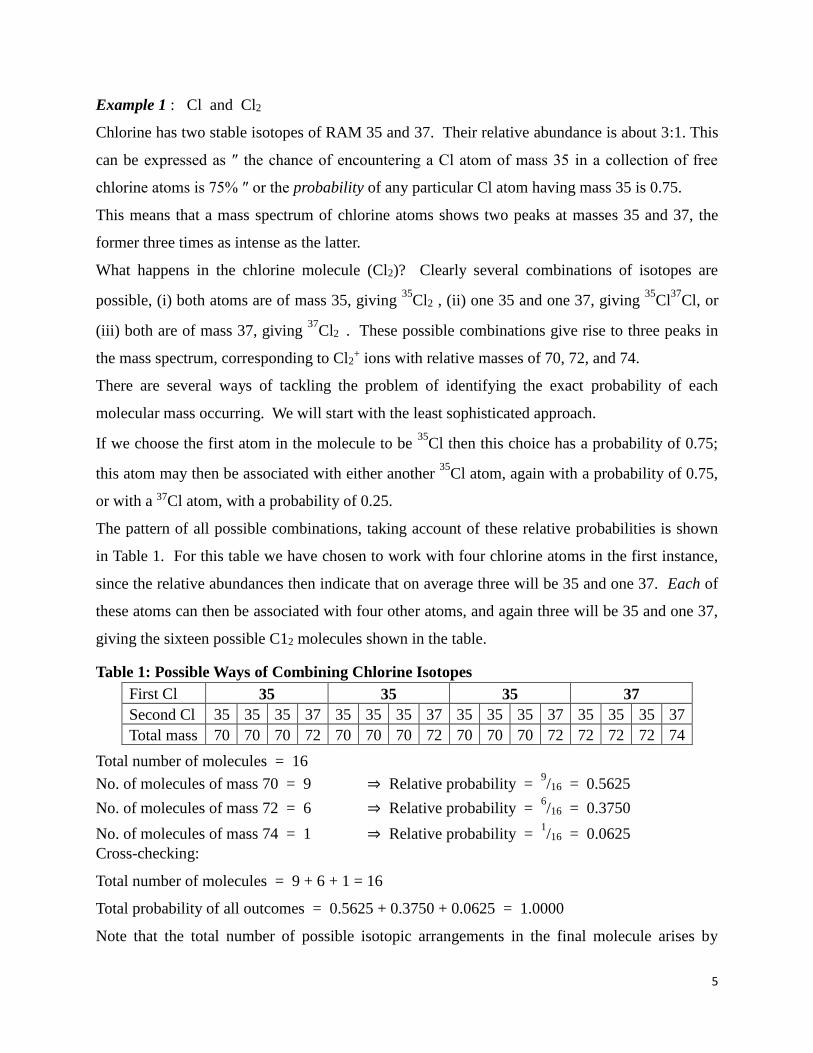
The pattern of all possible combinations, taking account of these relative probabilities is shown

in Table 1. For this table we have chosen to work with four chlorine atoms in the first instance,

since the relative abundances then indicate that on average three will be 35 and one 37. Each of

these atoms can then be associated with four other atoms, and again three will be 35 and one 37,

giving the sixteen possible C12 molecules shown in the table.

Table 1: Possible Ways of Combining Chlorine Isotopes

First Cl 35 35 35 37

Second Cl 35 35 35 37 35 35 35 37 35 35 35 37 35 35 35 37

Total mass 70 70 70 72 70 70 70 72 70 70 70 72 72 72 72 74

Total number of molecules = 16

No. of molecules of mass 70 = 9 ⇒ Relative probability = 9/16 = 0.5625

No. of molecules of mass 72 = 6 ⇒ Relative probability = 6/16 = 0.3750

No. of molecules of mass 74 = 1 ⇒ Relative probability = 1/16 = 0.0625

Cross-checking:

Total number of molecules = 9 + 6 + 1 = 16

Total probability of all outcomes = 0.5625 + 0.3750 + 0.0625 = 1.0000

Note that the total number of possible isotopic arrangements in the final molecule arises by

6

multiplying the number of choices for the first atom by the number of choices for the second. In

this case four for the first times four for the second i.e. sixteen.

If the only way in which these molecules can be distinguished is by mass then the relative

probabilities will be as shown on the right hand side of the lower part of the table – of the sixteen

arrangements, nine correspond to a total molecular mass of 70, six correspond to a total mass of

72 and one corresponds to a total mass of 74.

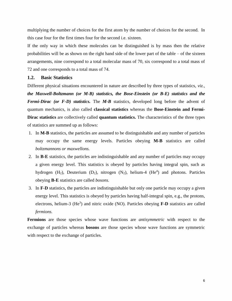
1.2. Basic Statistics

Different physical situations encountered in nature are described by three types of statistics, viz.,

the Maxwell-Boltzmann (or M-B) statistics, the Bose-Einstein (or B-E) statistics and the

Fermi-Dirac (or F-D) statistics. The M-B statistics, developed long before the advent of

quantum mechanics, is also called classical statistics whereas the Bose-Einstein and Fermi-

Dirac statistics are collectively called quantum statistics. The characteristics of the three types

of statistics are summed up as follows:

1. In M-B statistics, the particles are assumed to be distinguishable and any number of particles

may occupy the same energy levels. Particles obeying M-B statistics are called

boltzmannons or maxwellons.

2. In B-E statistics, the particles are indistinguishable and any number of particles may occupy

a given energy level. This statistics is obeyed by particles having integral spin, such as

hydrogen (H2), Deuterium (D2), nitrogen (N2), helium-4 (He4) and photons. Particles

obeying B-E statistics are called bosons.

3. In F-D statistics, the particles are indistinguishable but only one particle may occupy a given

energy level. This statistics is obeyed by particles having half-integral spin, e.g., the protons,

electrons, helium-3 (He3) and nitric oxide (NO). Particles obeying F-D statistics are called

fermions.

Fermions are those species whose wave functions are antisymmetric with respect to the

exchange of particles whereas bosons are those species whose wave functions are symmetric

with respect to the exchange of particles.

7

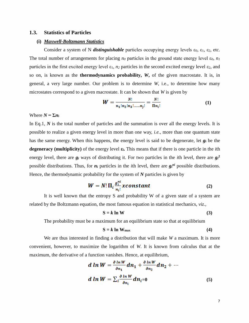
1.3. Statistics of Particles

(i) Maxwell-Boltzmann Statistics

Consider a system of N distinguishable particles occupying energy levels ε0, ε1, ε2, etc.

The total number of arrangements for placing n0 particles in the ground state energy level ε0, n1

particles in the first excited energy level ε1, n2 particles in the second excited energy level ε2, and

so on, is known as the thermodynamics probability, W, of the given macrostate. It is, in

general, a very large number. Our problem is to determine W, i.e., to determine how many

microstates correspond to a given macrostate. It can be shown that W is given by

(1)

Where N = Σni

In Eq.1, N is the total number of particles and the summation is over all the energy levels. It is

possible to realize a given energy level in more than one way, i.e., more than one quantum state

has the same energy. When this happens, the energy level is said to be degenerate, let gi be the

degeneracy (multiplicity) of the energy level εi. This means that if there is one particle in the ith

energy level, there are gi ways of distributing it. For two particles in the ith level, there are gi2

possible distributions. Thus, for ni particles in the ith level, there are gini possible distributions.

Hence, the thermodynamic probability for the system of N particles is given by

(2)

It is well known that the entropy S and probability W of a given state of a system are

related by the Boltzmann equation, the most famous equation in statistical mechanics, viz.,

S = k ln W (3)

The probability must be a maximum for an equilibrium state so that at equilibrium

S = k ln Wmax (4)

We are thus interested in finding a distribution that will make W a maximum. It is more

convenient, however, to maximize the logarithm of W. It is known from calculus that at the

maximum, the derivative of a function vanishes. Hence, at equilibrium,

=0 (5)

8

If we confine our investigation to a closed system of independent particles, it meets the

following two requirements:

(i) The total number of particles is constant, i.e.,

(6)

(ii) The total energy, U, of the system is constant, i.e.,

(7)

The constancy of the total number of particles implies that

(8)

And the constancy of the total energy implies that

(9)

From Eq. 2, taking logarithms both sides, we get

(10)

Using Stirling’s approximation according to which, for large x,

(11)

Using this approximation for , Eq. 10 becomes

(12)

Differentiating and bearing in mind that N and are constants, we get

(13)

Now, (14)

Hence, at equilibrium,

(15)

Eq. (15) gives the change in ln W which results when the number of particles in each energy

level is varied.

If our system were open, then would vary without restriction and the variations would

be independent of one another. It would then be possible to solve Eq. 15 by setting each of the

9

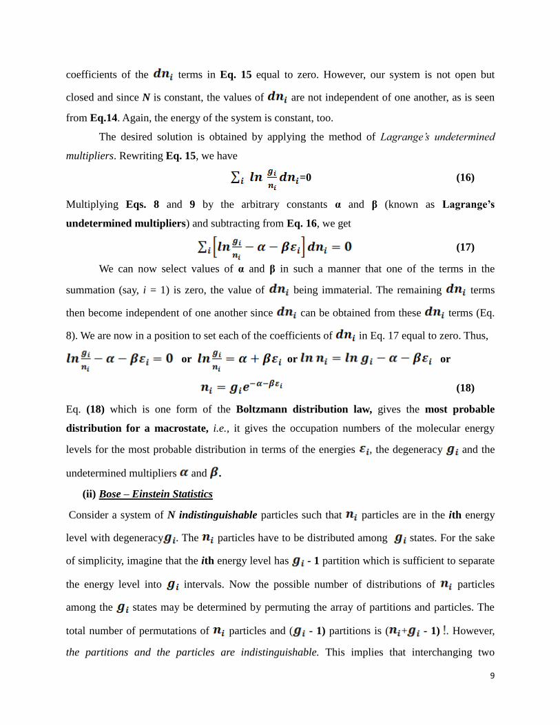
coefficients of the terms in Eq. 15 equal to zero. However, our system is not open but

closed and since N is constant, the values of are not independent of one another, as is seen

from Eq.14. Again, the energy of the system is constant, too.

The desired solution is obtained by applying the method of Lagrange’s undetermined

multipliers. Rewriting Eq. 15, we have

=0 (16)

Multiplying Eqs. 8 and 9 by the arbitrary constants α and β (known as Lagrange’s

undetermined multipliers) and subtracting from Eq. 16, we get

(17)

We can now select values of α and β in such a manner that one of the terms in the

summation (say, i = 1) is zero, the value of being immaterial. The remaining terms

then become independent of one another since can be obtained from these terms (Eq.

8). We are now in a position to set each of the coefficients of in Eq. 17 equal to zero. Thus,

or or or

(18)

Eq. (18) which is one form of the Boltzmann distribution law, gives the most probable

distribution for a macrostate, i.e., it gives the occupation numbers of the molecular energy

levels for the most probable distribution in terms of the energies , the degeneracy and the

undetermined multipliers and .

(ii) Bose – Einstein Statistics

Consider a system of N indistinguishable particles such that particles are in the ith energy

level with degeneracy . The particles have to be distributed among states. For the sake

of simplicity, imagine that the ith energy level has - 1 partition which is sufficient to separate

the energy level into intervals. Now the possible number of distributions of particles

among the states may be determined by permuting the array of partitions and particles. The

total number of permutations of particles and ( - 1) partitions is ( + - 1) . However,

the partitions and the particles are indistinguishable. This implies that interchanging two

10

partitions does not alter an arrangement; also interchanging two particles does not alter an

arrangement. Hence, we must divide is ( + - 1) by the number of permutations of the ( -

1) partitions, viz., ( - 1) and the number of permutations of particles, viz., to obtain

the number of possible arrangements of the particles in the energy level ε1. Thus,

The number of arrangements = (1)

As in the case of Maxwell – Boltzmann statistics, we assume that in the present case also the

total number of particles is constant and the total energy of the system is also constant, i.e.,

Thus, the thermodynamic probability W for the system of N particles (i.e., the number of ways

of distributing N particles among the various energy levels) is given by

(2)

Taking logarithms of both sides of Eq. 2, we get

(3)

Here, too, since and are very large numbers, we can invoke Stirling’s approximation, viz.,

, to obtain

(4)

Where we have set + - 1 = + and - 1 = . Since, is very large, it can be treated

as a continuous variable. Differentiation of Eq. 3, with respect to and setting the differential

equal to zero gives for the most probable thermodynamic state of the system,

or (5)

We know that,

(6)

(7)

Applying the method of Lagrange’s undetermined multipliers to Eqs. 5, 6 and 7, we get

(8)

11

Since the variations are independent of one another, hence

(9)

Whence (10)

(11)

Eq. 11 is the expression for the most probable distribution of N particles among the various

energy levels according to the Bose – Einstein statistics.

(iii) Fermi – Dirac Statistics

Consider that the particles are distributed among the states ( < ) where , as

before, is the degeneracy of the ith energy level. Imagine that the particles are indistinguishable.

This implies that the first particle may be placed in any one of the sates and for each one of

these choices, the second particle may be placed in any one of the remaining - 1 states, and so

on. Thus, the number of arrangements is given by the expression !/( - )!.Since the

particles are indistinguishable, the above expression has to be divided by the possible number of

permutations of particles, viz., !. Hence, the number of arrangements of particles in the

ith energy level is given by the expression, !/( !( - )!).

Thus, the thermodynamics probability W for the system of N particles (i.e., the number of

ways of distributing N particles among the various energy levels) is given by

(1)

Taking logarithms of both sides of Eq. 1, we have

(2)

Assuming that , and - are very large, we can apply Stirling’s approximation,

obtaining

(3)

Thus, for the post probable state,

12

or (4)

Since and ,

Hence, and (5)

Applying Lagrange’s method of undetermined multipliers, we obtain

(6)

Since the variations are independent of one another, hence.

or

or (7)

(8)

Eq. 8, is the expression for the most probable distribution of N particles among the energy levels

according to the Fermi – Dirac statistics.

1.4. Partition Function

In statistical mechanics, the partition function, q, is an important quantity that encodes the

statistical properties of a system in thermodynamic equilibrium. It is a function of temperature

and other parameters, such as the volume enclosing a gas. Most of the aggregate thermodynamic

variables of the system, such as the total energy, free energy, entropy, and pressure, can be

expressed in terms of the partition function or its derivatives.

There are actually several different types of partition functions, each corresponding to different

types of statistical ensemble (or, equivalently, different types of free energy.) The canonical

partition function applies to a canonical ensemble, in which the system is allowed to exchange

heat with the environment at fixed temperature, volume, and number of particles.

13

Suppose we have a thermodynamically large system that is in constant thermal contact with the

environment, which has temperature T, with both the volume of the system and the number of

constituent particles fixed. This kind of system is called a canonical ensemble. Let us label with

n (n = 1, 2, 3, ...) the exact states (microstates) that the system can occupy, and denote the total

energy of the system when it is in microstate n as En. Generally, these microstates can be

regarded as discrete quantum states of the system.

Canonical ensemble: The word ‘ensemble’ means ‘collection’ but it has been sharpened and

refined into a precise significance. The word ‘canon’ means ‘according to rule’. We take a closed

system of specified volume, composition and temperature which can be replicated to N times.

All the identical closed systems are regarded as being in thermal contact with one another, so

they can exchange energy. The total energy of all the systems is E and, because they are in

thermal equilibrium with one another, they all have the same temperature, T. This imaginary

collection of replications of the actual system with a common temperature is called the

Canonical ensemble.

The grand canonical partition function applies to a grand canonical ensemble, in which the

system can exchange both heat and particles with the environment, at fixed temperature, volume,

and chemical potential. Other types of partition functions can be defined for different

circumstances.

In the grand canonical ensemble the volume and temperature of each system is the same, but

they are open, which means that matter can be imagined as able to pass between the systems; the

composition of each one may fluctuate, but now the chemical potential is the same in each

system

14

There are two other important ensembles. They are micro canonical ensemble and grand

canonical ensemble. In the microcanonical ensemble the condition of constant temperature is

replaced by requirement that all the systems should have exactly the same energy; each system is

individually isolated.

Micro canonical Ensemble: N, V, E common

Canonical ensemble: N, V, T common

Grand canonical ensemble: μ, V, T common

Since an ensemble is a collection of imaginary replications of the system, so we are free to let the

number of members be as large as we like; when appropriate, we can let N become infinite. The

number of members of the ensemble in a state with energy Ei is donated ni, and we can speak of

the configuration of the ensemble.

1.5. Thermodynamic Functions

We can use the Boltzmann distribution law and the related partition functions to calculate the

macroscopic (thermodynamic) properties such as internal energy, enthalpy, entropy, free energy,

etc., of matter from molecular properties. The partition functions are, therefore, of great

importance in statistical thermodynamics.

Internal Energy, U: The internal energy, U, of a system consisting of N independent particles

(atoms or molecules) is equal to the sum of the energies of individual particles. Thus,

(1)

Where is the average energy of the particles defined by

(2)

Now, (3)

15

where the differentiation is carried out at constant volume since the energies depend upon the

volume. Hence,

(4)

Therefore, from Eqs. 1 and 4 for a system containing N particles,

(5)

Since and Nk = nR (where n is the number of moles), we have

Or (6)

Molar Heat Capacity, : For one mole of a system (n = 1), differentiation of U with respect to

T at constant V, yields the molar heat capacity . Hence,

(7)

Entropy, S: If the particles are considered indistinguishable, then the thermodynamic probability

for the system, must be divided by to yield the new thermodynamic probability of the

Boltzmann distribution as

(8)

Using the Boltzmann equation for entropy, viz.,

(9)

We have, (10)

Using the Stirling approximation, viz.,

(11)

We obtain (12)

Since,

Substituting in Eq. 12, we have

(13)

For n moles of the system, kN = nR. Also, using the expression for U given by Eq. 6, we have

16

(14)

Helmholtz Function or Work Function, A: A = U – TS

Hence, after substituting for U from Eq. 6 and for S from Eq. 14,

We have

(15)

Since nR = Nk, we can write Eq. 15 as

(16)

(17)

Where Q is the molar partition function, i.e., the partition function for one mole, viz., for

Avogadro’s number of particles and q is the molecular partition function, viz., the partition

function for a single molecule.

Pressure, P: By definition, pressure is given by

(18)

Differentiating Eq. 16 with respect to V at constant T, we have

(19)

(20)

Gibbs Function, G: The Gibbs free energy defined as

G = H – TS = (U + PV) – TS = A + PV

Substituting Eq. 15 for A and Eq. 20 for P, we obtain

(21)

Enthalpy, H: Enthalpy is defined as H = U + PV

Substituting Eq. 6 for U and Eq. 20 for P, we have

(22)

The chemical potential

In equilibrium, a system is in steady state. Thus, a simple chemical reaction in equilibrium, of the

form

17

A ⇌ B (1)

has to have as many molecules going from A → B as from B → A in equilibrium. Another way

to say this is that there should be no change in free energy for a reacting molecule, or that the

total chemical potential (change in free energy per molecule) is zero

μA = μB (2)

in equilibrium. The equilibrium condition can be related to the free energy for the different

ensembles by

(3)

For gas phase reactions in the Canonical ensemble, where A = −kT lnQ, and the

chemical potential is

(4)

using Stirling’s approximation, lnN! = N lnN − N. This gives a simple relation for reacting gas

particles, for which the system partition function Q = QAQB is the product of the partition

function for each species. In this case, the condition for equilibrium

(5)

where NA and NB are the number of A and B molecules respectively

The equilibrium constant

The equilibrium condition can be written as a constant with respect to N because qA and qB are

both single particle partition functions with no N dependence

(6)

The equilibrium constant can also be written in terms of concentrations, which are independent

of volume. Substituting the density ρ = N/V

(7)

18

The single particle partition function q is equal to the volume times a function of T, so that q/V is

independent of volume, which makes KC also a constant with respect to volume. For simple

reactions, given by Eq. 7, these two constants are equal, KN = KC.

We can also find an equilibrium pressure constant, using the ideal gas relation PV = NkT,

(8)

which again reduces to KN and KC.

Thermodynamic Properties of an Ideal Monoatomic Gas

A monoatomic gas, such as helium, neon, argon, etc., has only translational and electronic degree

of freedom. Hence, molecular partition function is given by

However, we know that

where is the degeneracy of the electronic ground state. Hence

Using Eq. for

Taking for most atomic systems,

According to Eq. 6,

The molar heat capacity is given by

Entropy is obtained by substituting Eq. 29 in Eq. 15

19

For one mole of an ideal gas,

Substituting in Eq. 32 and simplifying, we get

From Eq. 22, the pressure is given by

which is the equation of state for n moles of an ideal gas.

Substituting Eqs. 30 and 34, in the relation , we have

From Eq. 17, the Helmholtz function

Using Eq. 28 and the equation of state, PV = RT, we have

From Eqs. 37 and 23, the Gibbs function for an ideal gas is given by

This is further simplified to give

Statistical Derivation of the Equation of State for Non-ideal Fluids

How can a gas have three different volumes at the same time? The answer is that the term

“fluid,” meaning that which flows, is more general than “gas.” the term fluid includes both

liquids and gases sometimes we call it non-ideal gas.

20

The relation between pressure p and partition function Q is a very important route to the

equations of state of real gases in terms of intermolecular forces, for the latter can be built into Q.

The partition function for a gas of independent particles leads to the perfect gas equation of state,

pV = nRT. Real gases differ from perfect gases in their equations of state.

where B is the second virial coefficient and C is the third virial coefficient.

The total kinetic energy of a gas is the sum of the kinetic energies of the individual molecules.

Therefore, even in a real gas the canonical partition function factorizes into a part arising from

the kinetic energy, which is the same as for the perfect gas, and a factor called the configuration

integral, Z, which depends on the intermolecular potentials.

Where Λ the thermal de Broglie wavelength: By comparing this equation with (Q = qN/N!, with q

= V/Λ3), we see that for a perfect gas of atoms (with no contributions from rotational or

vibrational modes)

For a real monatomic gas (for which the intermolecular interactions are isotropic), Z is related to

the total potential energy Ep of interaction of all the particles by

where dτi is the volume element for atom i. The physical origin of this term is that the probability

of occurrence of each arrangement of molecules possible in the sample is given by a Boltzmann

distribution in which the exponent is given by the potential energy corresponding to that

arrangement.

The second virial coefficient then turns out to be

The quantity f is the Mayer f-function: it goes to zero when the two particles are so far apart that

Ep = 0. When the intermolecular interaction depends only on the separation r of the particles and

21

not on their relative orientation or their absolute position in space, as in the interaction of closed-

shell atoms in a uniform sample, the volume element simplifies to 4πr2dr (because the integrals

over the angular variables in dτ = r2dr sin θ dθdφ give a factor of 4π).

How this equation is used by considering the hard-sphere potential, which is infinite when the

separation of the two molecules, r, is less than or equal to a certain value σ, and is zero

for greater separations. Then

This calculation of B raises the question as to whether a potential can be found that, when the

virial coefficients are evaluated, gives the van der Waals equation of state.

Such a potential can be found for weak attractive interactions (a << RT): it consists of a hard-

sphere repulsive core and a long-range, shallow attractive region. A further point is that, once a

second virial coefficient has been calculated for a given intermolecular potential, it is possible to

calculate other thermodynamic properties that depend on the form of the potential. For example,

it is possible to calculate the isothermal Joule–Thomson coefficient, μT from the thermodynamic

relation.

Equilibrium Constants for Gas Phase Reactions

Classical thermodynamics is very useful when applied to chemical or physical processes that are

in a state of equilibrium. How well does statistical thermodynamics apply to equilibrium?

Where A and B represent reactants, C and D are the products, and A, B, C, and D are the molar

coefficients of the balanced chemical reaction.

22

Algebraically,

It is the convention to subtract the reactants from the products.

The overall partition function of the system Qsys can be written as the product of the molecular

partition functions of each component:

In this equation, we are labeling each molecular partition function with the label of the relevant

component. Also, each component is occupying the same volume and has the same temperature

(otherwise the system is not at equilibrium), but that each component has its own characteristic

amount Ni at equilibrium. Statistical thermodynamics gives an expression for the chemical

potential of a component:

where in the case of a multicomponent mixture, the partial derivative is taken with respect to

only one component, Ni, and the other components remain as constants. This has the effect of

eliminating all other species’ partition functions from the evaluation of each particular i.

Substituting for each in equation

The -kT terms cancel to yield

23

We can use the properties of logarithms to take each coefficient and make it an exponent inside

the logarithm term.

using the rule that lna + lnb = ln ab

If the logarithms of two products are the same (as the above equation indicates), then the

arguments of the two individual logarithms are the same. Another way to put this is that we can

take the inverse logarithm of both sides of the above equation and still have an equality.

At this point, we will rearrange equation to bring all of the partition functions Qi to one side and

all of the amounts Ni to the other. The exponents vi will appear on both sides (as a consequence

of the algebra of exponents).

The partition functions Qi are constants that are characteristic of each chemical species, and the

coefficients vi are characteristic of the balanced chemical reaction. Therefore, the left side of

equation is some constant that is characteristic of the chemical reaction. This Equation

shows that the characteristic of constant is related to the amounts of each chemical species when

the reaction reaches chemical equilibrium, even though each individual Qi itself is defined in

terms of the molecule, not any extent of reaction! Since the fraction in terms of the Qi values has

a characteristic value, then the fraction in terms of the amounts Ni at equilibrium must also have

a characteristic value. This value is called the equilibrium constant for the reaction.

For an ideal gas, the partition function Q is a simple function of volume (again, from qtrans) times

a more complicated function of temperature (fromseveral other q’s):

It is convenient to divide each molecular Q by volume to get a volume independent partition

function:

24

By substituting this volume-independent partition function into the partition function expression

for the equilibrium constant, labeled K(T), which is characteristic of the chemical species in the

reaction and dependent solely on T.

Equilibrium constants can also be expressed in terms of the partial pressures of the gas-phase

reactants and products. The pressure-base equilibrium constant, Kp, is related to Kc by the

expression

where vi represents the proper combination of the stoichiometric coefficients of gas-phase

substances in the balanced chemical reaction. Remember that vi values are positive for products

and negative for reactants.

25

Surface Chemistry

Topic to be covered:

2. Interfacial Structure

2.1. Surface Tension and Surface Free Energy

2.2. Methods of Surface Tension Measurement

2.3. Nature and Thermodynamics of Liquid-Gas Interface

2.4. The Surface Tension of Solutions

2.5. Surfaces of Solids

2.6. Adsorption at the Solid Solution Interface

Introduction

Surface chemistry can be roughly defined as the study of chemical reactions at interfaces. It

is closely related to surface engineering, which aims at modifying the chemical composition of a

surface by incorporation of selected elements or functional groups that produce various desired

effects or improvements in the properties of the surface or interface. Surface chemistry also

overlaps with electrochemistry. Surface science is of particular importance to the field

of heterogeneous catalysis.

In this chapter we will discuss the physical chemistry of surfaces in a broad sense. Although

an obvious enough point, it is perhaps worth noting that in reality we will always be dealing with

the interface between two phases (liquid-gas, solid-liquid and solid-gas) and that, in general, the

properties of an interface will be affected by physical or chemical changes in either of the two

phases involved.

2. Interfacial Structure

A phase defined as a part of a system that was "homogeneous throughout." Such a definition

implies that the matter deep in the interior of a phase is subject to exactly the same conditions as

the matter at the exterior which forms the surface. An interface is a surface forming a common

boundary among two different phases of matter, such as an insoluble solid and a liquid, two

immiscible liquids, a liquid and an insoluble gas or a liquid and vacuum. The importance of the

interface depends on the type of system: the bigger the quotient area/volume, the more effect the

surface phenomena will have. This is clearly impossible in any case, since the molecules (or

26

ions) in the interior are surrounded on all sides by the uniform field of force of neighbor

molecules (or ions) of the same substance. The molecules at the surface were bounded on one

side by neighbors of the same kind but on the other side by an entirely different sort of

environment.

Consider, for example, the surface of a liquid in contact with its vapor, shown in figure below. A

molecule in the interior of the liquid is in a uniform field of force. A molecule at the surface is

subject to a net attraction toward the bulk of the liquid, which is not compensated by an equal

attraction from the more highly dispersed vapor molecules. Thus all liquid surfaces, in the absence of

other forces, tend to contract to the minimum area. For example, freely suspended volumes of liquid

assume a spherical shape, since the sphere has the minimum surface-to-volume ratio.

Figure: Liquid-vapor interfaces.

In order to extend the area of an interface like that in figure that is to bring molecules from the

interior into the surface, works must be done against the cohesive forces in the liquid. It follows

that the surface portions of the liquid have a higher free energy than the bulk liquid. This extra

surface free energy is more usually described by saying that there is a surface tension, acting

parallel to the surface, which opposes any attempt to extend the interface.

2.1. Surface Tension and Surface Free Energy

Although referred to as a free energy per unit area, surface tension may equally well be thought

of as a force per unit length. Two serve to illustrate these viewpoints. Consider, first, a soap film

stretched over a wire frame, one end of which is movable (Fig.). Experimentally one observes

that a force is acting on the movable member in the direction opposite to that of the arrow in the

diagram. If the value of the force per unit length is denoted by , then the work done is extending

the movable member a distance dx is

Work = ldx = dA (1)

27

Where dA = ldx is the change in area. In the second formulation, appears to be energy per unit

area.

A second illustration involves the soap bubble. We will choose to think of in terms of energy

per unit area. In the absence of gravitational or other fields, a soap bubble is spherical, as this is

the shape of minimum surface area for an enclosed volume. A soap bubble of radius r has a total

surface free energy of 4r2 and, if the radius were to decrease by dr, then the change in surface

free energy would be 8rdr. Since shrinking decreases the surface energy, the tendency to do so

must be balanced by a pressure difference across the film

Figure: A soap film stretched across a wire frame with one movable side.

P such that the work against this pressure P4r2dr is just equal to the decrease in surface free

energy. Thus

P4r2dr = 8rdr (2)

Or

P = 2/r (3)

One thus arrives at the important conclusion that the smaller the bubble, the greater the pressure

of the air inside relative to that outside.

The forgoing examples illustrate the point that equilibrium surfaces may be treated using either

the mechanical concept of surface tension or the mathematically equivalent concept of surface

free energy. A similar duality of viewpoint can be argued on a molecular scale so that the

decision as to whether surface tension or surface free energy is the more fundamental concept

becomes somewhat a matter of individual taste. The term surface tension is the older of the two;

it goes back to early ideas that the surface of a liquid had some kind of contractile “skin”.

Surface free energy implies only that work is required to bring molecules from the interior of the

phase to the surface. Table given below shows surface tension of some liquids.

28

2.2. Methods of Surface Tension Measurement

(i) Capillary-rise Method

A capillary tube of radius r is vertically inserted into a liquid. The liquid rises to a height h and forms a

concave meniscus. The surface tension () acting along the inner circumference of the tube exactly

supports the weight of the liquid column.

By definition, surface tension is force per 1 cm acting at a tangent to the meniscus surface. If the angle

between the tangent and the tube wall is , the vertical component of surface tension is cos . The total

surface tension along the circular contact line of meniscus is 2r times. Therefore,

Upward force = 2r cos

where r is the radius of the capillary. For most liquids, is essentially zero, and cos = 1. Then the

upward force reduces to 2r.

The downward force on the liquid column is due to its weight which is mass × gravity. Thus,

Downward force = hr2 dg

where d is the density of the liquid.

But

Upward force = Downward force

or 2r = hr2 dg

= hrdg/2

In order to know the value of , the value of h is found with the help of a travelling microscope and

density (d) with a pyknometer.

29

Figure: (a) Rise of liquid in a capillary tube; (b) Surface tension () acts along tangent to meniscus and

its vertical component is Cos ; (c) Upward force 2rCos counter balances the downward force due

to weight of liquid column, r2 hgd.

PROBLEM 1. A capillary tube of internal diameter 0.21 mm is dipped into a liquid whose density is 0.79

g cm–3. The liquid rises in this capillary to a height of 6.30 cm. Calculate the surface tension of the liquid.

(g = 980 cm sec–2).

SOLUTION

We know:

= hrdg/2

Where, h = height of liquid in capillary in centimeters; r = radius of capillary in centimeters; d = density

of liquid in g cm–1; g = acceleration due to gravity in cm sec–2

Substituting the values from the above example, h = 6.30 cm

r = 0.21/2x1/10 = 0.0105 cm

d = 0.79g.cm-3

g = 980cm.sec-2

Substituting these in above eq.

= (6.30x0.0105x0.79x980)/2

= 25.6 dynescm-1

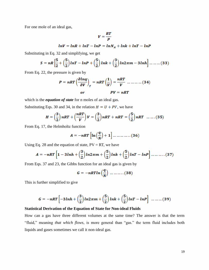
(ii) Drop Formation Method

A drop of liquid is allowed to form at the lower end of a capillary tube. The drop is supported by the

upward force of surface tension acting at the outer circumference of the tube. The weight of the drop (mg)

pulls it downward. When the two forces are balanced, the drop breaks. Thus at the point of breaking,

m g = 2 r (1)

where m = mass of the drop; g = acceleration due to gravity; r = outer radius of the tube

30

The apparatus employed is a glass pipette with a capillary at the lower part. This is called a

Stalagmometer or Drop pipette. It is cleaned, dried and filled with the experimental liquid, say upto

mark A. Then the surface tension is determined by one of the two methods given below.

(a) Drop-weight Method. About 20 drops of the given liquid are received from the drop-pipette in a

weighing bottle and weighed. Thus weight of one drop is found. The drop-pipette is again cleaned and

dried. It is filled with a second reference liquid (say water) and weight of one drop determined as before.

Then from equation (1)

m1 g = 2 r 1 (2)

m2 g = 2 r 2 (3)

Dividing (2) by (3)

1/2 = m1/ m2

Knowing the surface tension of reference liquid from Tables, that of the liquid under study can be found.

(b) Drop-number Method. The drop-pipette is filled upto the mark A with the experimental liquid

(No.1). The number of drops is counted as the meniscus travels from A to B. Similarly, the pipette is

filled with the reference liquid (No.2) as the meniscus passes from A to B. Let n1 and n2 be the number of

drops produced by the same volume V of the two liquids. Thus,

The volume of one drop of liquid 1 = V/n1

The mass of one drop of liquid 1 = (V/n1)d1

where d1 is the density of liquid 1.

Similarly,

The mass of one drop of liquid 2 = (V/n2)d2

Then from equation (4)

1/2 = (V/n1)d1/(V/n2)d2 = n2d1/ n1d2

31

The value of d1 is determined with a pyknometer. Knowing d2 and 2 from reference tables, 1 can be

calculated.

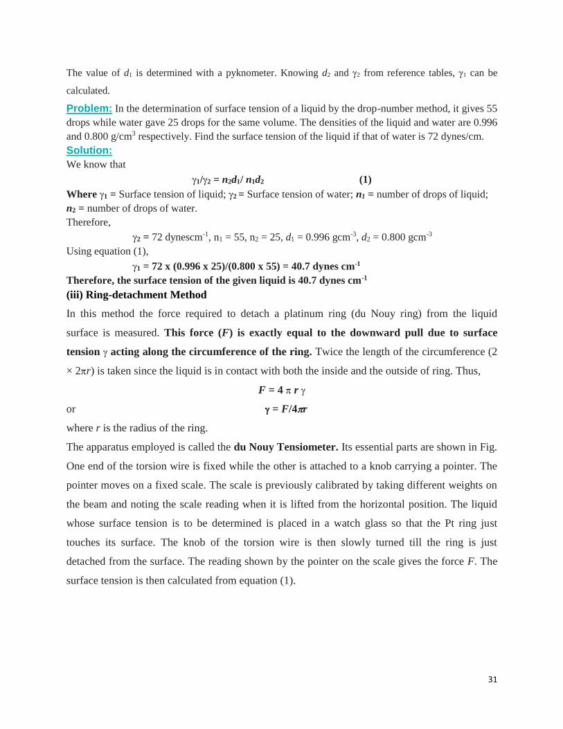
Problem: In the determination of surface tension of a liquid by the drop-number method, it gives 55

drops while water gave 25 drops for the same volume. The densities of the liquid and water are 0.996

and 0.800 g/cm3 respectively. Find the surface tension of the liquid if that of water is 72 dynes/cm.

Solution:

We know that

1/2 = n2d1/ n1d2 (1)

Where 1 = Surface tension of liquid; 2 = Surface tension of water; n1 = number of drops of liquid;

n2 = number of drops of water.

Therefore,

2 = 72 dynescm-1, n1 = 55, n2 = 25, d1 = 0.996 gcm-3, d2 = 0.800 gcm-3

Using equation (1),

1 = 72 x (0.996 x 25)/(0.800 x 55) = 40.7 dynes cm-1

Therefore, the surface tension of the given liquid is 40.7 dynes cm-1

(iii) Ring-detachment Method

In this method the force required to detach a platinum ring (du Nouy ring) from the liquid

surface is measured. This force (F) is exactly equal to the downward pull due to surface

tension acting along the circumference of the ring. Twice the length of the circumference (2

× 2r) is taken since the liquid is in contact with both the inside and the outside of ring. Thus,

F = 4 r

or = F/4r

where r is the radius of the ring.

The apparatus employed is called the du Nouy Tensiometer. Its essential parts are shown in Fig.

One end of the torsion wire is fixed while the other is attached to a knob carrying a pointer. The

pointer moves on a fixed scale. The scale is previously calibrated by taking different weights on

the beam and noting the scale reading when it is lifted from the horizontal position. The liquid

whose surface tension is to be determined is placed in a watch glass so that the Pt ring just

touches its surface. The knob of the torsion wire is then slowly turned till the ring is just

detached from the surface. The reading shown by the pointer on the scale gives the force F. The

surface tension is then calculated from equation (1).

32

du Nouy Tensiometer

du Nouy ring with a suspending

hook.

2.3. Nature and Thermodynamics of Liquid-Gas Interface

The surface tension is a definite and accurately measureable property of the interface between

liquid phases. Moreover, its value is very rapidly established in pure substances of ordinary

viscosity; dynamic methods indicate that a normal surface tension is established within a

millisecond and probably sooner. Thus it is appropriate to discuss the thermodynamic basic for

surface tension.

Surface Thermodynamic Quantities for a pure Substance

A hypothetical system consisting of some liquid that fills a box having a sliding cover; the

material of the cover is such that the interfacial tension between it and the liquid is zero. If the

cover is slid back so as to uncover an amount of surface dA, the work required to do so will be

dA. This is reversible work at constant pressure and temperature and thus gives the increase in

free energy of the system.

dG = dA (1)

The total free energy of the system is then made up of the molar free energy times the total

number of moles of the liquid plus Gs, the surface free energy per unit area, times the total

surface area. Thus

,

s

T P

dGG

dA

(2)

Because this process is a reversible one, the heat associated with it gives the is surface entropy

dq = T dS = TSsdA (3)

33

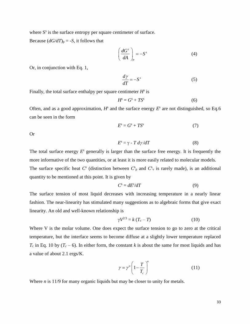
where Ss is the surface entropy per square centimeter of surface.

Because (dG/dT)p = -S, it follows that

ss

P

dGS

dA

(4)

Or, in conjunction with Eq. 1,

sdS

dT

(5)

Finally, the total surface enthalpy per square centimeter Hs is

Hs = Gs + TSs (6)

Often, and as a good approximation, Hs and the surface energy Es are not distinguished, so Eq.6

can be seen in the form

Es = Gs + TSs (7)

Or

Es = - T d /dT (8)

The total surface energy Es generally is larger than the surface free energy. It is frequently the

more informative of the two quantities, or at least it is more easily related to molecular models.

The surface specific heat Cs (distinction between Csp and Cs

v is rarely made), is an additional

quantity to be mentioned at this point. It is given by

Cs = dEs/dT (9)

The surface tension of most liquid decreases with increasing temperature in a nearly linear

fashion. The near-linearity has stimulated many suggestions as to algebraic forms that give exact

linearity. An old and well-known relationship is

V2/3 = k (Tc – T) (10)

Where V is the molar volume. One does expect the surface tension to go to zero at the critical

temperature, but the interface seems to become diffuse at a slightly lower temperature replaced

Tc in Eq. 10 by (Tc – 6). In either form, the constant k is about the same for most liquids and has

a value of about 2.1 ergs/K.

1

n

o

c

T

T

(11)

Where n is 11/9 for many organic liquids but may be closer to unity for metals.

34

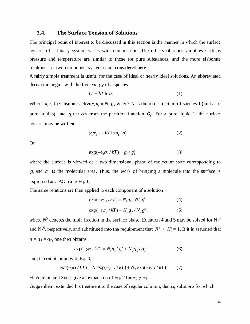
2.4. The Surface Tension of Solutions

The principal point of interest to be discussed in this section is the manner in which the surface

tension of a binary system varies with composition. The effects of other variables such as

pressure and temperature are similar to those for pure substances, and the more elaborate

treatment for two-component system is not considered here.

A fairly simple treatment is useful for the case of ideal or nearly ideal solutions. An abbreviated

derivation begins with the free energy of a species

lni iG kT a (1)

Where ia is the absolute activity, i i ia N g , where iN is the mole fraction of species I (unity for

pure liquids), and ig derives from the partition function iQ . For a pure liquid 1, the surface

tension may be written as

1 1 1 1ln / skT a a (2)

Or

1 1 1 1exp( / ) / skT g g (3)

where the surface is viewed as a two-dimensional phase of molecular state corresponding to

1

sg and 1 is the molecular area. Thus, the work of bringing a molecule into the surface is

expressed as a G using Eq. 1.

The same relations are then applied to each component of a solution

1 1 1 1 1exp( / ) / s skT N g N g (4)

2 2 2 2 2exp( / ) / s skT N g N g (5)

where NS denotes the mole fraction in the surface phase. Equation 4 and 5 may be solved for N1S

and N2S, respectively, and substituted into the requirement that 1

sN + 2

sN = 1. If it is assumed that

= 1 = 2, one then obtains

1 1 1 2 2 2exp( / ) / /s skT N g g N g g (6)

and, in combination with Eq. 3,

1 1 2 2exp( / ) exp( / ) exp( / )kT N kT N kT (7)

Hildebrand and Scott give an expansion of Eq. 7 for 1 ≠ 2.

Guggenheim extended his treatment to the case of regular solution, that is, solutions for which

35

2

1 2lnRT f N 2

2 1lnRT f N (8)

where f denotes the activity coefficient. A very simple relationship for such regular solutions

comes from Prigogine and Defay:

= 1N1 + 2N2 – βN1N2 (9)

where β is a semi-empirical constant.

2.5. Surfaces of Solids

A solid, by definition, is a portion of matter that is rigid and resists stress. Although the surface

of a solid must, in principle, be characterized by surface free energy, it is evident that the usual

methods of capillarity are not very useful since they depend on measurements of equilibrium

surface properties given Laplace’s equation. Since a child deforms in an elastic manner, its shape

will be determined more by its past history than by surface tension forces.

Surface growth

A simple picture of a perfect crystal surface is as a tray of oranges in a grocery store (Fig. 1). A

gas molecule that collides with the surface can be imagined as a table-tennis ball bouncing

erratically over the oranges. The molecule loses energy as it bounces under the influence of

intermolecular forces, but it is likely to escape from the surface before it has lost so much kinetic

energy that is has become trapped. The same is true, to some extent, of an ionic crystal in contact

with a solution. There is little energy advantage for an ion in solution to discard some of its

solvating molecules and stick at an exposed position on a flat surface.

Fig. 1: A schematic diagram of the flat surface of a solid.

The picture changes when the surface has defects, for then there are ridges of incomplete layers

of atoms or ions. A typical type of surface defect is a step between two otherwise flat layers of

atoms called terraces (Fig. 2). A step defect might itself have defects, including kinks. When an

atom settles on a terrace it migrates across it under the influence of the intermolecular potential,

and might come to a step or a corner formed by a kink. Instead of interacting with a single

36

terrace atom, the molecule now interacts with several, and the interaction may be strong enough

to trap it. Likewise, when ions deposit from solution, the loss of the solvation interaction is offset

by a strong Coulombic interaction between the arriving ions and several ions at the surface

defect.

Fig. 2: Some of the kinds of defects that may occur on otherwise perfect terraces. Defects play

an important role in surface growth and catalysis.

The rapidity of growth depends on the crystal plane concerned and—perhaps surprisingly—the

slowest growing faces dominate the appearance of the crystal. This feature is explained in Fig. 3,

where we see that although the horizontal face grows forward most rapidly, it grows itself out of

existence and the more slowly growing faces survive.

Fig. 3: The slower-growing faces of a crystal dominate its final external appearance. Three

successive stages of the growth are shown.

Surface Composition and structure

Under normal conditions, a surface exposed to a gas is constantly bombarded with molecules and

a freshly prepared surface is covered very quickly. Just how quickly can be estimated by using

the kinetic theory of gases and the following expression for the collision flux, ZW, the number of

hits on a region of a surface during an interval divided by the area of the region and the duration

of the interval:

37

1/ 2

2w

b

pZ

mk T (1)

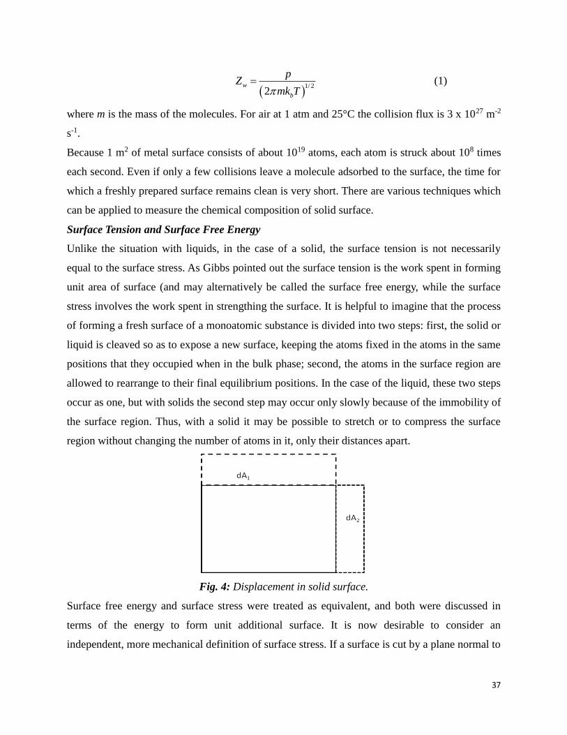
where m is the mass of the molecules. For air at 1 atm and 25°C the collision flux is 3 x 1027 m-2

s-1.

Because 1 m2 of metal surface consists of about 1019 atoms, each atom is struck about 108 times

each second. Even if only a few collisions leave a molecule adsorbed to the surface, the time for

which a freshly prepared surface remains clean is very short. There are various techniques which

can be applied to measure the chemical composition of solid surface.

Surface Tension and Surface Free Energy

Unlike the situation with liquids, in the case of a solid, the surface tension is not necessarily

equal to the surface stress. As Gibbs pointed out the surface tension is the work spent in forming

unit area of surface (and may alternatively be called the surface free energy, while the surface

stress involves the work spent in strengthing the surface. It is helpful to imagine that the process

of forming a fresh surface of a monoatomic substance is divided into two steps: first, the solid or

liquid is cleaved so as to expose a new surface, keeping the atoms fixed in the atoms in the same

positions that they occupied when in the bulk phase; second, the atoms in the surface region are

allowed to rearrange to their final equilibrium positions. In the case of the liquid, these two steps

occur as one, but with solids the second step may occur only slowly because of the immobility of

the surface region. Thus, with a solid it may be possible to stretch or to compress the surface

region without changing the number of atoms in it, only their distances apart.

Fig. 4: Displacement in solid surface.

Surface free energy and surface stress were treated as equivalent, and both were discussed in

terms of the energy to form unit additional surface. It is now desirable to consider an

independent, more mechanical definition of surface stress. If a surface is cut by a plane normal to

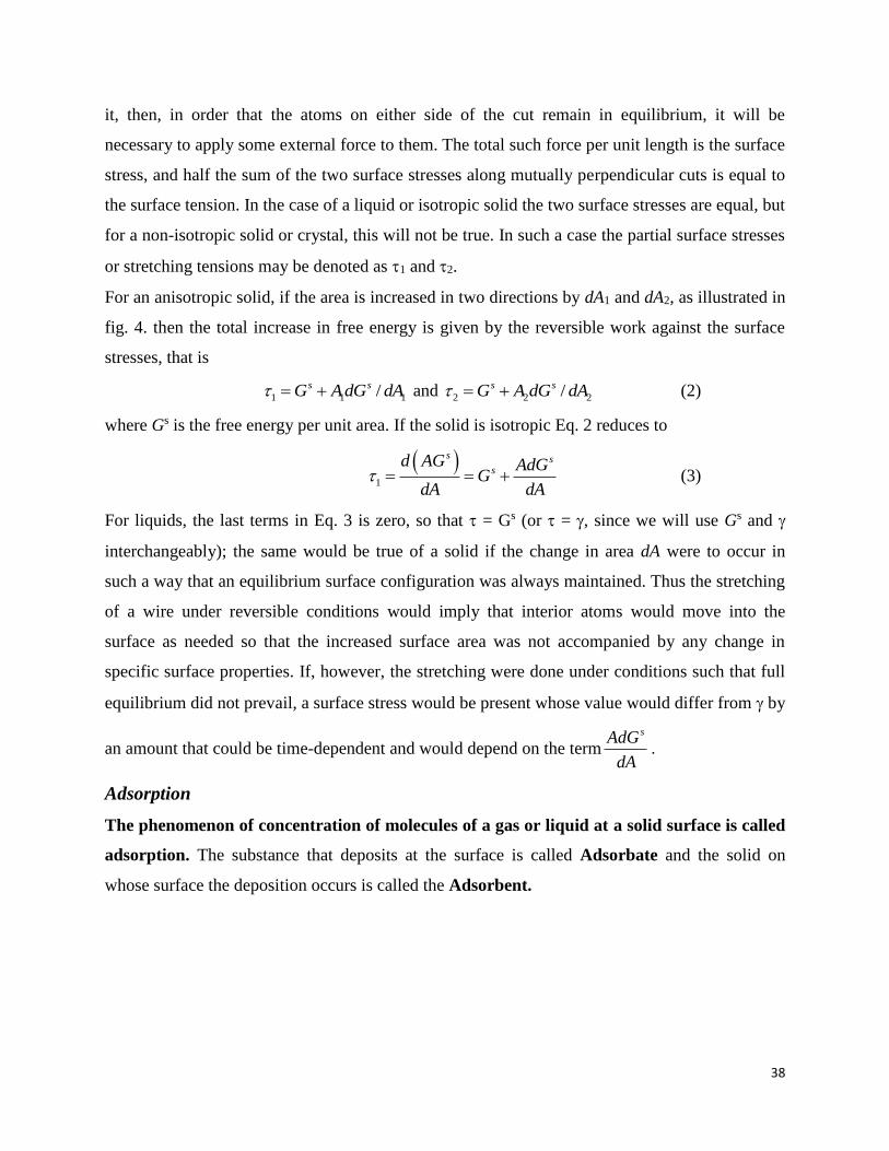
38

it, then, in order that the atoms on either side of the cut remain in equilibrium, it will be

necessary to apply some external force to them. The total such force per unit length is the surface

stress, and half the sum of the two surface stresses along mutually perpendicular cuts is equal to

the surface tension. In the case of a liquid or isotropic solid the two surface stresses are equal, but

for a non-isotropic solid or crystal, this will not be true. In such a case the partial surface stresses

or stretching tensions may be denoted as 1 and 2.

For an anisotropic solid, if the area is increased in two directions by dA1 and dA2, as illustrated in

fig. 4. then the total increase in free energy is given by the reversible work against the surface

stresses, that is

1 1 1/s sG AdG dA and 2 2 2/s sG A dG dA (2)

where Gs is the free energy per unit area. If the solid is isotropic Eq. 2 reduces to

1

s ss

d AG AdGG

dA dA (3)

For liquids, the last terms in Eq. 3 is zero, so that = Gs (or = , since we will use Gs and

interchangeably); the same would be true of a solid if the change in area dA were to occur in

such a way that an equilibrium surface configuration was always maintained. Thus the stretching

of a wire under reversible conditions would imply that interior atoms would move into the

surface as needed so that the increased surface area was not accompanied by any change in

specific surface properties. If, however, the stretching were done under conditions such that full

equilibrium did not prevail, a surface stress would be present whose value would differ from by

an amount that could be time-dependent and would depend on the termsAdG

dA.

Adsorption

The phenomenon of concentration of molecules of a gas or liquid at a solid surface is called

adsorption. The substance that deposits at the surface is called Adsorbate and the solid on

whose surface the deposition occurs is called the Adsorbent.

39

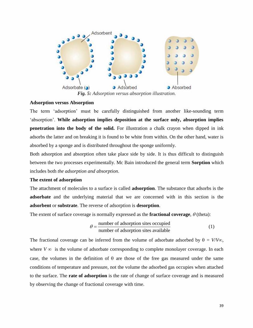
Fig. 5: Adsorption versus absorption illustration.

Adsorption versus Absorption

The term ‘adsorption’ must be carefully distinguished from another like-sounding term

‘absorption’. While adsorption implies deposition at the surface only, absorption implies

penetration into the body of the solid. For illustration a chalk crayon when dipped in ink

adsorbs the latter and on breaking it is found to be white from within. On the other hand, water is

absorbed by a sponge and is distributed throughout the sponge uniformly.

Both adsorption and absorption often take place side by side. It is thus difficult to distinguish

between the two processes experimentally. Mc Bain introduced the general term Sorption which

includes both the adsorption and absorption.

The extent of adsorption

The attachment of molecules to a surface is called adsorption. The substance that adsorbs is the

adsorbate and the underlying material that we are concerned with in this section is the

adsorbent or substrate. The reverse of adsorption is desorption.

The extent of surface coverage is normally expressed as the fractional coverage, (theta):

number of adsorption sites occupied

number of adsorption sites available (1)

The fractional coverage can be inferred from the volume of adsorbate adsorbed by = V/V,

where V is the volume of adsorbate corresponding to complete monolayer coverage. In each

case, the volumes in the definition of are those of the free gas measured under the same

conditions of temperature and pressure, not the volume the adsorbed gas occupies when attached

to the surface. The rate of adsorption is the rate of change of surface coverage and is measured

by observing the change of fractional coverage with time.

40

Physisorption and Chemisorptions

Molecules and atoms can attach to surfaces in two ways, although there is no clear frontier

between the two types of adsorption. In physisorption (an abbreviation of ‘physical

adsorption’), there is a van der Waals interaction between the adsorbate and the substrate (for

example, a dispersion or a dipolar interaction of the kind responsible for the condensation of

vapors to liquids). The energy released when a molecule is physisorbed is of the same order of

magnitude as the enthalpy of condensation. Such small energies can be absorbed as vibrations of

the lattice and dissipated as thermal motion, and a molecule bouncing across the surface will

gradually lose its energy and finally adsorb to it in the process called accommodation. The

enthalpy of physisorption can be measured by monitoring the rise in temperature of a sample of

known heat capacity, and typical values are in the region of -20 kJ mol-1 (Table 1). This small

enthalpy change is insufficient to lead to bond breaking, so a physisorbed molecule retains its

identity but might be distorted. Enthalpies of physisorption may also be measured by observing

the temperature dependence of the parameters that occur in the adsorption isotherm.

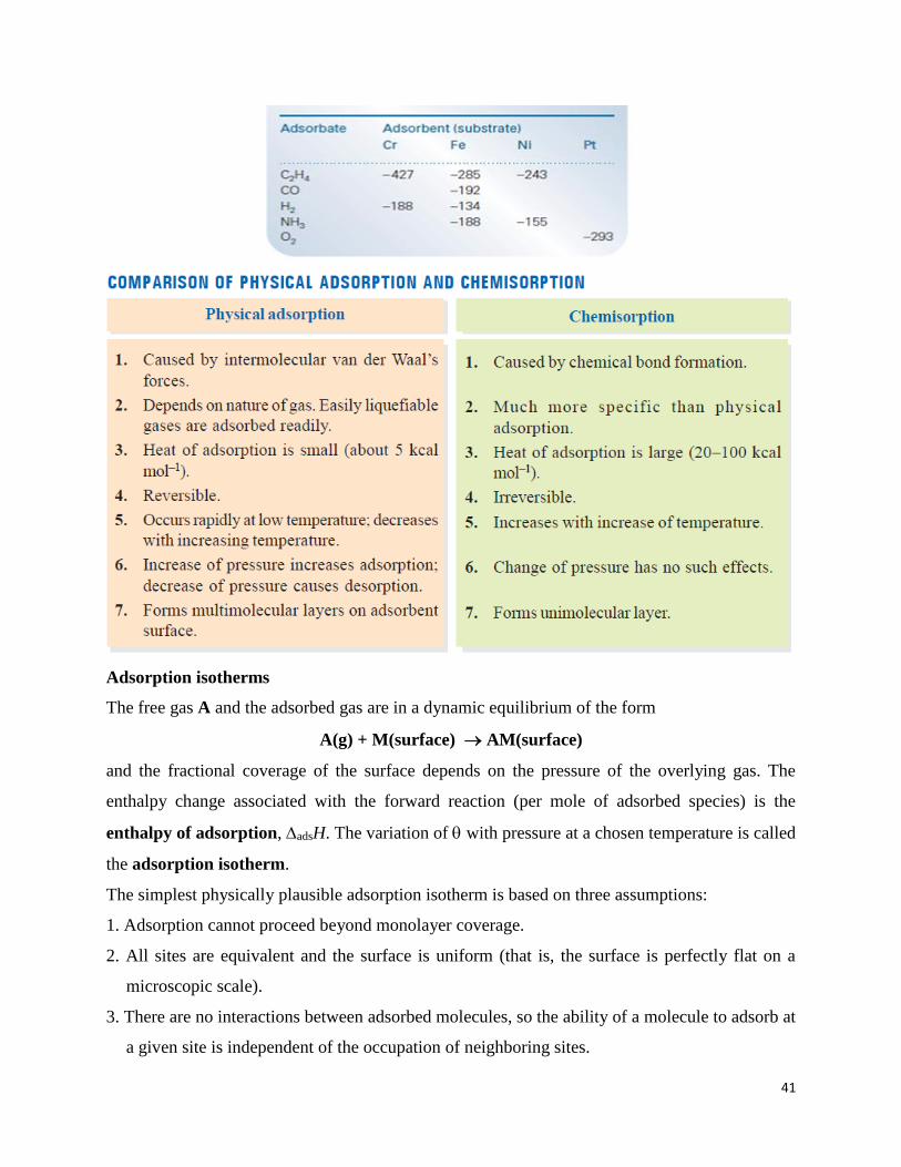
Table 1: Maximum observed enthalpies of physisorption, 1/( )o

ads adsH kJmol

In chemisorption (an abbreviation of ‘chemical adsorption’), the molecules (or atoms) adsorb to

the surface by forming a chemical (usually covalent) bond and tend to find sites that maximize

their coordination number with the substrate. The enthalpy of chemisorption is much more

negative than that for physisorption, and typical values are in the region of -200 kJ mol-1 (Table

2). The distance between the surface and the closest adsorbate atom is also typically shorter for

chemisorption than for physisorption. A chemisorbed molecule may be torn apart at the demand

of the unsatisfied valencies of the surface atoms and the existence of molecular fragments on the

surface as a result of chemisorption is one reason why solid surfaces catalyse reactions.

Table 2: Enthalpies of chemisorption, 1/( )o

ads adsH kJmol

41

Adsorption isotherms

The free gas A and the adsorbed gas are in a dynamic equilibrium of the form

A(g) + M(surface) AM(surface)

and the fractional coverage of the surface depends on the pressure of the overlying gas. The

enthalpy change associated with the forward reaction (per mole of adsorbed species) is the

enthalpy of adsorption, adsH. The variation of with pressure at a chosen temperature is called

the adsorption isotherm.

The simplest physically plausible adsorption isotherm is based on three assumptions:

1. Adsorption cannot proceed beyond monolayer coverage.

2. All sites are equivalent and the surface is uniform (that is, the surface is perfectly flat on a

microscopic scale).

3. There are no interactions between adsorbed molecules, so the ability of a molecule to adsorb at

a given site is independent of the occupation of neighboring sites.

42

Assumptions 2 and 3 imply, respectively, that the enthalpy of adsorption is the same for all sites

and is independent of the extent of surface coverage. The relation between the fractional

coverage and the partial pressure of A, p, that results from these three assumptions is the

Langmuir isotherm:

1

Kp

Kp

a

b

kK

k (2)

where ka and kb are, respectively, the rate constants for adsorption and desorption. This

expression is plotted for various values of K (which has the dimensions of 1/pressure) in Fig. 6.

We see that as the partial pressure of A increases, the fractional coverage increases towards 1.

Half the surface is covered when p = 1/K. At low pressures (in the sense that Kp << 1), the

denominator can be replaced by 1, and θ = Kp. Under these conditions, the surface coverage

increases linearly with pressure. At high pressure (in the sense that Kp >> 1), the 1 in the

denominator can be neglected, the Kp cancel, and θ = 1. Now the surface is saturated.

Fig. 6: Langmuir isotherm for nondissociative adsorption for different values of K.

A further point is that because K is essentially an equilibrium constant, then its temperature

dependence is given by the van’t Hoff equation :

'

'

1 1ln ln adsHK K

R T T

(3)

It follows that if we plot ln K against 1/T, then the slope of the graph is equal to −ΔadsH /R, where

ΔadsH is the standard enthalpy of adsorption. However, because this quantity might vary with the

extent of surface coverage either because the adsorbate molecules interact with each other or

because adsorption occurs at a sequence of different sites, care must be taken to measure K at the

same value of the fractional coverage. The resulting value of ΔadsH is called the isosteric

43

enthalpy of adsorption. The variation of ΔadsH with θ allows us to explore the validity of the

assumptions on which the Langmuir isotherm is based. There are two modifications of the

Langmuir isotherm that should be noted. Suppose the substrate dissociates on adsorption, as in

A2(g) + M(surface) A–M(surface) + A–M(surface)

The resulting isotherm is

1/ 2

1/ 21

Kp

Kp

(4)

The second modification we need to consider deals with a mixture of two gases A and B that

compete for the same sites on the surface. To show that if A and B both follow Langmuir

isotherms, and adsorb without dissociation, then

1

A AA

A A B B

K p

K p K p

,

1

B BB

A A B B

K p

K p K p

(5)

where KJ (with J = A or B) is the ratio of adsorption and desorption rate constants for species J,

pJ is its partial pressure in the gas phase, and θJ is the fraction of total sites occupied by J.

Coadsorption of this kind is important in catalysis and we use these isotherms later.

The rates of surface processes

Figure 7, shows how the potential energy of a molecule varies with its distance above the

adsorption site. As the molecule approaches the surface its potential energy decreases as it

becomes physisorbed into the precursor state for chemisorption. Dissociation into fragments

often takes place as a molecule moves into its chemisorbed state, and after an initial increase of

energy as the bonds stretch there is a sharp decrease as the adsorbate–substrate bonds reaches

their full strength. Even if the molecule does not fragment, there is likely to be an initial increase

of potential energy as the bonds adjust when the molecule approaches the surface.

44

Fig. 7: The potential energy profiles for the dissociative chemisorption of an A2 molecule. In

each case, P is the enthalpy of (nondissociative) physisorption and C that for chemisorption (at T

= 0). The relative locations of the curves determine whether the chemisorption is (a) not

activated or (b) activated.

In most cases, therefore, we can expect there to be a potential energy barrier separating the

precursor and chemisorbed states. This barrier, though, might be low and might not rise above

the energy of a distant, stationary molecule (as in Fig. 7a). In this case, chemisorption is not an

activated process and can be expected to be rapid. Many gas adsorptions on clean metals appear

to be nonactivated. In some cases the barrier rises above the zero axis (as in Fig 7b); such

chemisorptions are activated and slower than the nonactivated kind. An example is the

adsorption of H2 on copper, which has an activation energy in the region of 20–40 kJ mol−1.

One point that emerges from this discussion is that rates are not good criteria for distinguishing

between physisorption and chemisorption. Chemisorption can be fast if the activation energy is

small or zero; but it may be slow if the activation energy is large. Physisorption is usually fast,

but it can appear to be slow if adsorption is taking place on a porous medium.

The rate at which a surface is covered by adsorbate depends on the ability of the substrate to

dissipate the energy of the incoming molecule as thermal motion as it crashes on to the surface.

If the energy is not dissipated quickly, the molecule migrates over the surface until a vibration

expels it into the overlying gas or it reaches an edge. The proportion of collisions with the

surface that successfully lead to adsorption is called the sticking probability, s:

rate of adsorption of particles by the surface

rate of collision of particles with the surfaces (6)

The denominator can be calculated from kinetic theory, and the numerator can be measured by

observing the rate of change of pressure. Values of s vary widely. For example, at room

temperature CO has s in the range 0.1–1.0 for several d-metal surfaces, suggesting that almost

every collision sticks, but for N2 on rhenium s < 10−2, indicating that more than a hundred

collisions are needed before one molecule sticks successfully.

Desorption is always an activated process because the molecules have to be lifted from the foot

of a potential well. A physisorbed molecule vibrates in its shallow potential well, and might

shake itself off the surface after a short time. The temperature dependence of the first-order rate

of departure can be expected to be Arrhenius-like,

/dE RT

dk Ae

(7)

45

where A is a pre-exponential factor and the activation energy for desorption, Ed, is likely to be

comparable to the enthalpy of physisorption. In the discussion of half-lives of first-order

reactions is t1/2 = (ln 2)/k; so for desorption, the half-life for remaining on the surface has a

temperature dependence given by

/

1/ 2

ln 2dE RT

o

d

t ek

, ln 2

oA

(8)

(Note the positive sign in the exponent: the half-life decreases as the temperature is raised.) If we

suppose that 1/τ0 is approximately the same as the vibrational frequency of the weak molecule–

surface bond (about 1012 Hz) and Ed ≈ 25 kJ mol−1, then residence half-lives of around 10 ns are

predicted at room temperature. Lifetimes close to 1 s are obtained only by lowering the

temperature to about 100 K. For chemisorption, with Ed = 100 kJ mol−1 and guessing that τ0 =

10−14 s (because the adsorbate–substrate bond is quite stiff), we expect a residence half-life of

about 3 × 103 s (about an hour) at room temperature, decreasing to 1 s at about 350 K.

One way to measure the desorption activation energy is to monitor the rate of increase in

pressure when the sample is maintained at a series of temperatures and then to attempt to make

an Arrhenius plot. A more sophisticated technique is temperature programmed desorption

(TPD) or thermal desorption spectroscopy (TDS). The basic observation is a surge in

desorption rate (as monitored by a mass spectrometer) when the temperature is raised linearly to

the temperature at which desorption occurs rapidly; but once desorption has occurred there is no

more adsorbate to escape from the surface, so the desorption flux falls again as the temperature

continues to rise. The TPD spectrum, the plot of desorption flux against temperature, therefore

shows a peak, the location of which depends on desorption activation energy. There are three

maxima in the example shown in Fig. 8, indicating the presence of three adsorption sites with

different activation energies.

46

Fig. 8: The flash desorption spectrum of H2 on the face of tungsten.

Catalytic activity at surfaces

A catalyst acts by providing an alternative reaction path with lower activation energy. A catalyst

does not disturb the final equilibrium composition of the system, only the rate at which that

equilibrium is approached. In this section we shall consider heterogeneous catalysis, in which

the catalyst and the reagents are in different phases. A common example is a solid introduced as

a heterogeneous catalyst into a gas-phase reaction. Many industrial processes make use of

heterogeneous catalysts, which include platinum, rhodium, zeolites, and various metal oxides,

but increasingly attention is turning to homogeneous catalysts, partly because they are easier to

cool. However, their use typically requires additional separation steps, and such catalysts are

generally immobilized on a support, in which case they become heterogeneous. In general,

heterogeneous catalysts are highly selective and to find an appropriate catalyst each reaction

must be investigated individually.

Computational procedures are beginning to be a fruitful source of prediction of catalytic activity.

A metal acts as a heterogeneous catalyst for certain gas-phase reactions by providing a surface to

which a reactant can attach by chemisorption. For example, hydrogen molecules may attach as

atoms to a nickel surface and these atoms react much more readily with another species (such as

an alkene) than the original molecules. The chemisorption step therefore results in a reaction

pathway with lower activation energy than in the absence of the catalyst. Note that

chemisorption is normally required for catalytic activity: physisorption might precede

chemisorption but is not itself sufficient.

47

Mechanisms of heterogeneous catalysis

Heterogeneous catalysis normally depends on at least one reactant being adsorbed (usually

chemisorbed) and modified to a form in which it readily undergoes reaction. Often this

modification takes the form of a fragmentation of the reactant molecules. The catalyst ensemble

is the minimum arrangement of atoms at the surface active site that can be used to model the

action of the catalyst. It may be determined, for instance, by diluting the active metal with a

chemically inert metal and observing the catalytic activity of the resulting alloy. In this way it

has been found, for instance, that as many as 12 neighboring Ni atoms are needed for the

cleavage of the C—C bond in the conversion of ethane to methane.

The decomposition of phosphine (PH3) on tungsten is first-order at low pressures and zeroth-

order at high pressures. To account for these observations, we write down a plausible rate law in

terms of an adsorption isotherm and explore its form in the limits of high and low pressure. If the

rate is supposed to be proportional to the surface coverage and we suppose that θ is given by the

Langmuir isotherm, we would write

1

rr

k KpRate k

Kp

(9)

where p is the pressure of phosphine and kr is a rate constant. When the pressure is so low that

Kp << 1, we can neglect Kp in the denominator and obtain

rRate k Kp (10)

and the decomposition is first-order. When Kp >> 1, we can neglect the 1 in the denominator,

whereupon the Kp terms cancel and we are left with

rRate k (11)

and the decomposition is zeroth-order. Many heterogeneous reactions are first-order, which

indicates that the rate-determining stage is the adsorption process.

In the Langmuir–Hinshelwood mechanism (LH mechanism) of surface-catalysed

reactions, the reaction takes place by encounters between molecular fragments and atoms

adsorbed on the surface. We therefore expect the rate law to be overall second order in the extent

of surface coverage:

A + B P Rate = krθAθB

48

Insertion of the appropriate isotherms for A and B then gives the reaction rate in terms of the

partial pressures of the reactants. For example, if A and B follow the adsorption isotherms given

in eqn 4, then the rate law can be expected to be

2(1 )

r A B A B

A A B B

k K K p pRate

K p K p

(12)

The parameters K in the isotherms and the rate constant kr are all temperature dependent, so the

overall temperature dependence of the rate may be strongly non-Arrhenius, in the sense that the

reaction rate is unlikely to be proportional to e−Ea/RT. The LH mechanism is dominant for the

catalytic oxidation of CO to CO2 on the surface of platinum.

In the Eley–Rideal mechanism (ER mechanism) of a surface-catalysed reaction, a gas-

phase molecule collides with another molecule already adsorbed on the surface. We can

therefore expect the rate of formation of product to be proportional to the partial pressure, pB, of

the nonadsorbed gas B and the extent of surface coverage, A, of the adsorbed gas A. It follows

that the rate law should be

A + B P Rate = krpBθA

The rate constant, kr, might be much larger than for the uncatalysed gas-phase reaction because

the reaction

on the surface has a low activation energy and the adsorption itself is often not activated. If we

know the adsorption isotherm for A, we can express the rate law in terms of its partial pressure,

pA. For example, if the adsorption of A follows a Langmuir isotherm in the pressure range of

interest, then the rate law would be

1

r A B

A

k Kp pRate

Kp

(13)

If A were a diatomic molecule that adsorbed as atoms, then we would substitute the isotherm

given in eqn 4 instead. According to eqn 13, when the partial pressure of A is high (in the sense

KpA >> 1) there is almost complete surface coverage, and the rate law is

r A Br B

A

k Kp pRate k p

Kp (14)

Now the rate-determining step is the collision of B with the adsorbed fragments. When the

pressure of A is low (KpA << 1), perhaps because of its reaction, the rate law becomes

49

1

r A Br A B

k Kp pRate k Kp p (15)

Now the extent of surface coverage is rate determining. Almost all thermal surface-catalysed

reactions are thought to take place by the LH mechanism, but a number of reactions with an ER

mechanism have also been identified from molecular beam investigations.

2.6. Adsorption at the Solid Solution Interface

Adsorption of a solute from a solution onto a solid adsorbent is more difficult to treat

theoretically than the corresponding adsorption of gases on solids. It appears however that in this

case, too, like the gas-solid adsorption, a monomolecular layer is formed. The solvating power of

the solvent inhibits the formation of a multilayer.

For adsorption from solutions, a commonly used isotherm is the Freundlich adsorption isotherm.

If x is the mass of the solute adsorbed on mass m of adsorbent and c is the concentration of the

solute in the solution, then the Freundlich adsorption isotherm is expressed as

/ nx m a kc (1)

where k and n are empirical constants. Taking logs,

ln ln lna k n c (2)

This logarithmic form is convenient to use. If we plot ln a versus ln c, the plot would be a

straight line with slope equal to n and intercept equal to ln k.

The Gibbs Adsorption Isotherm for Adsorption from solutions

The concentration of a solute at the surface of a solution is, in general, markedly different from

that in the bulk. If the surface tension of the solute is lower than that of the liquid, it tends to

accumulate at the surface of the liquid thereby decreasing the surface tension (or the surface free

energy per unit area) of the liquid. A quantitative treatment of the thermodynamics of adsorption

of a solute at the surface of a liquid was given in 1878 by J.W.Gibbs, the greatest 19th century

American mathematical physicist.

For a system containing two components, the Gibbs free energy can be written as

1 1 2 2G n n (3)

Where n1 and n2 are the amounts (number of moles), 1 and 2 are the chemical potentials (i.e.,

partial molar Gibbs free energies) of the two components, respectively. Since we are dealing with

the adsorption of one of the components on the surface which results in changing the surface free

energy, Eq.3 is modified to

50

1 1 2 2G n n (4)

Where is the surface energy which is numerically the same as the surface tension and is the

surface area. The complete differential of Eq. 4 is written as

1 1 1 1 2 2 2 2dG n d dn n d dn d d (5)

We see that free energy G now depends upon five independent variables, viz., T, P, n1, n2 and .

Thus,

1 2( , , , , )G f T P n n (6)

1 2 1 2 2 22 1

1 2

, , , , , , , , ,1 2, , , , , ,P n n T n n P T n nP T n P T n

G G G G GdG dT dP dn dn d

T P n n

(7)

According to thermodynamics, the partial derivatives

1 2 1 2 2 22 1, , , , , , , , ,1 2, , , , , ,

, , ,P n n T n n P T n nP T n P T n

G G G G Gand

T P n n

Eq. 7 are, respectively, equal to S, V, 1, 2 and .

Hence, 1 1 2 2dG SdT VdP dn dn d (8)

At constant temperature (dT = 0) and at constant pressure (dP = 0), Eq. 8 reduces to

, 1 1 2 2( )T PdG dn dn d (9)

From Eqs. 5 and 9.

1 1 2 2 0n d n d d (10)

The corresponding expression for the bulk of the liquid is

1 1 2 2 0o on d n d (11)

Where 1

on and 2

on are the amounts (number of moles) of the liquid and the solute, respectively, in

the bulk phase.

Since the system is in equilibrium, the chemical potential of each component in the bulk and the

surface phase must be the same. The system, on being disturbed, attains a new equilibrium so

that the changes in the chemical potentials must be identical in both the phases, i.e., d1 and d2

in Eqs. 10 and 11 must be identical. Elimination of d2 from these equations gives

1 2 1 2 2 2/ 0o on n n d n d d

Or 2 1 2 1 2( / ) 0o on n n n d d

51

Or 2 1 2 1

2

( / )o on n n nd

d

(12)

The quantity within parenthesis of Eq. 12 gives the amount 2

on of solute 2 associated with the

amount 1

on of liquid 1 in the bulk phase. On the other hand, n2 is the amount of the solute

associated with the amount n1 of the liquid at the surface. Thus, the numerator on the right hand

side of Eq. 12 gives the excess amount of the solute present in the surface of the solute per unit

area of the surface, designated as 2 , i.e., 2 1 2 1 2[ ( / )]/o on n n n . Thus, from Eq. 12,

2

2

d

d

(13)

The chemical potential of solute 2 is given by

2 2 2( ) lnl RT a (14)

where 2 ( )l is the chemical potential of the pure solute in the liquid phase. Hence,

2 2lnd RTd a 2[ ( ) 0]d l Q (15)

Substituting for d2 in Eq. 13, we obtain

22

2 2

1

lnT T

a

RT a RT a

(16)

When the solution is very dilute, it behaves ideally so that the activity a2 of the solute can be

replaced by its concentration c2. Thus,

22

2 2

1

lnT T

c

RT c RT c

(17)

Eq. 17 is called Gibbs adsorption isotherm. Knowing the concentration-dependence of , 2 can

be calculated. For a solute that lowers the surface tension, the surface excess concentration 2 is

positive and for a solute that raises the surface tension, 2 is negative.