statistical techniques
DESCRIPTION
Statistical Techniques. MAR 6648: Marketing Research February 1, 2011. Overview. We’ll talk about basic statistical tools T-tests, crosstabs, and regression are useful tools We’ll talk about what they can and can’t do More sophisticated tools can give a deeper view of your customers - PowerPoint PPT PresentationTRANSCRIPT

Statistical Techniques
MAR 6648: Marketing ResearchFebruary 1, 2011

Overview
• We’ll talk about basic statistical tools– T-tests, crosstabs, and regression are useful tools
• We’ll talk about what they can and can’t do
• More sophisticated tools can give a deeper view of your customers– Conjoint analysis, cluster analysis, and factor
analysis can help you understand who your customers are and what they like

A Quick Note on Data Analysis
• Statistics are just one part of an argument• People are easily persuaded by numbers and statistics
– The more complicated the analysis, the less likely it is to be challenged
• The strongest challenge to many statistical arguments is not in how the data are analyzed, but in how the data are collected– Methodological expertise always trumps data analytic
experience– Data analytic knowledge allows for more careful
consideration of methodology
Really Basic: Comparing Groups
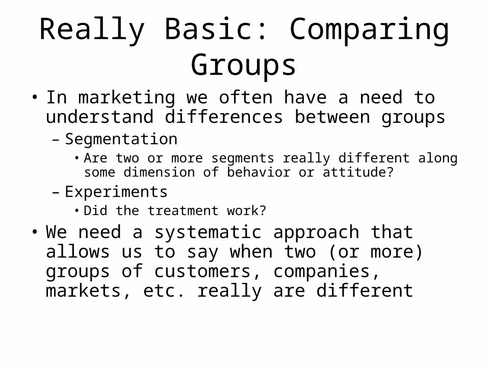
• In marketing we often have a need to understand differences between groups– Segmentation
• Are two or more segments really different along some dimension of behavior or attitude?
– Experiments• Did the treatment work?
• We need a systematic approach that allows us to say when two (or more) groups of customers, companies, markets, etc. really are different

Most Basic: t-tests
• Do web shoppers pay a different price for cars than dealership shoppers?
• Do a hypothesis test:
=Null Hypothesis:
≠Alternative:

T-test Results
• “Customers who bought their new vehicles on the Auto Online website report having paid less for their vehicles than did customers who purchased their vehicles at the dealership (Monline = $11,582 vs. Mdealer = $13,594), t(1398) = -6.14, p < .001).”– If the p-value of the test is “small” we reject the null
hypothesis– Here “small” typically means less than 5% (p = .05)
• Now try answering a different question:– Are customers who purchase a car online more likely to
buy their next car online as well?

Understanding Associations
• One of the most common questions in Marketing Research:– Are two (or more) variables associated?
Customer type
Subsequent transaction

Tools for Analyzing Associations
• Cross tabulation– Only for two categorical
variables– Easy to understand
• Regression– Applies to any number
of variables– Not necessarily
categorical variables– Slightly harder to
understand
0
200
400
600
800
1000
1200
1400
0.75 1.25 1.75 2.25 2.75 3.25
Price
Sal
es
Online 1st Dealer 1st
Online 2nd
Dealer 2nd
Χ2-test for Association
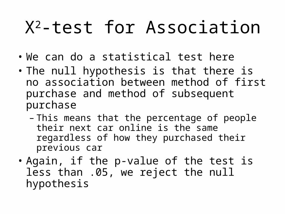
• We can do a statistical test here• The null hypothesis is that there is no
association between method of first purchase and method of subsequent purchase– This means that the percentage of people their
next car online is the same regardless of how they purchased their previous car
• Again, if the p-value of the test is less than .05, we reject the null hypothesis

Intuition for Χ2-test
• The Χ2-test is based on comparing the actual cell counts to what we would expect them to be if there was no association
1 2
= 154/500
= 333/500
3 4
= 0.692*0.666 = 0.231*500
We would expect the table to looklike this if there was no association

Intuition for Χ2-test
• The Χ2-test is based on comparing the actual cell counts to what we would expect them to be if there was no association
Actual Expected
Conclusion: Based on this data, it looks like customers who purchase a car online are no more likely to buy their next car online than customers who bought their initial car from a dealer.
Χ2 (1, N = 500) = 3.002, p = .08

Crosstabs
• Crosstabs is a quick and easy tool for analyzing the association between two categorical variables
• Caveats:– You find associations – not causations
• An observed association may be driven by a third variable not captured in the analysis
• In crosstabs we cannot control for other variables – we need regression for this
– Warning: Be careful when cell counts are low. The test does not work well in this case (stats programs should tell you)

Key Points• T-tests:
– Good for analyzing data with a continuous dependent variable and a 2-level categorical variable
– Does not allow for a more complex design– Does not allow the analysis to control for the
presence of another known variable• Crosstabs
– An easy method for describing categorical data– Easily analyzed using simple non-parametric tests
(e.g., chi-square)– Poorly suited for handling non-categorical data– But often unable to isolate causation in data

Regression
• Regression analysis is widely used in Marketing Research– It can detect associations between variables– It can help make forecasts– It can test Marketing Mix models: Impact of
marketing mix variables on sales– It can analyze results of experiments

Example: Minute Maid Sales
• Imagine that you’ve been hired as a consultant for the Minute Maid Company
• Before going for an important meeting with senior management, you have been asked to analyze the sales data for MM orange juice for the Southern California market
• To assist in your deliberations, some data have become available from one of your key accounts (the largest grocery chain in the market)

Example: Minute Maid Sales
• The database was collected from weekly store scanner data that captures information such as sales (# of cartons sold), price, and other promotion information for each product
• Management is particularly interested in understanding how different pricing strategies affect sales

The data
week Total OJ Sales(00 cartons) Minute Maid-Sales (00 cartons) Price-MM
1 1029 66 2.99
2 350 89 2.99
3 802 565 2.59
4 701 50 2.99
5 484 186 2.99
6 763 334 2.39
7 848 57 2.99
8 957 732 1.99
. . . .
. . . .
115 1296 88 2.53
116 1472 760 2.19

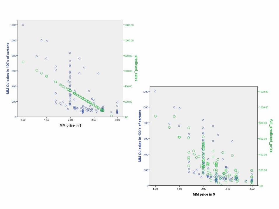
Weekly Minute Maid Sales and Price
A Linear Sales Model
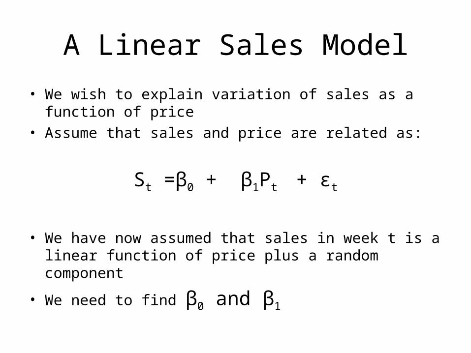
• We wish to explain variation of sales as a function of price• Assume that sales and price are related as:
St =β0 + β1Pt + εt
• We have now assumed that sales in week t is a linear function of price plus a random component
• We need to find β0 and β1

SPSS Regression output
Test of H0: β1=0Ha: β1 ≠0
p-valuet-statistic
b1
b0
Standard errors of b0 and b1 ≈ uncertainty associated withb0,b1
St =β0 + β1Pt + εt

What does this mean?
Key Points
• Regression:– Generates a specific equation describing the
relationship between a specific predictor (e.g., prices) and a specific outcome variable (e.g., sales)
– The results can offer precise (if imperfect) prescriptions for managers

Example: Minute Maid Sales
• We previously identified a relationship between Minute Maid prices and Minute Maid sales– Essentially, Sales = 1093 + (-377 x price)
• This model seems a little simplistic– What about accounting for the behavior of
competitors?– Regression is good at that too
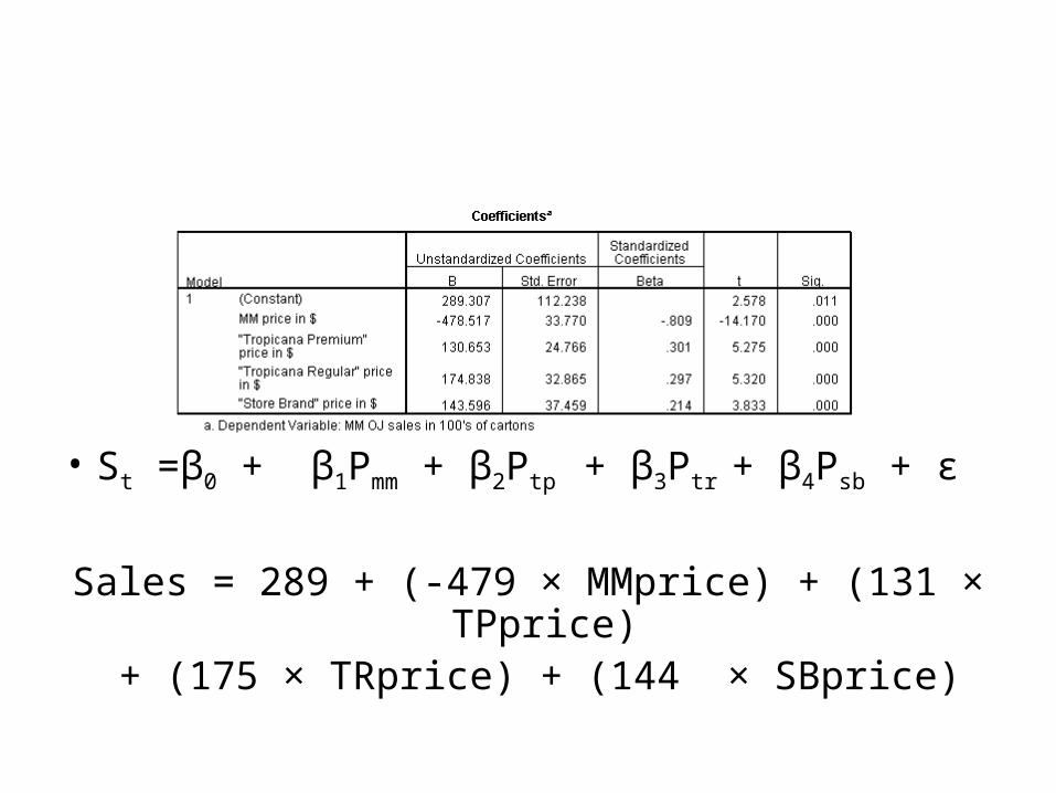
• St =β0 + β1Pmm + β2Ptp + β3Ptr + β4Psb + ε
Sales = 289 + (-479 × MMprice) + (131 × TPprice) + (175 × TRprice) + (144 × SBprice)

These are dummy coded variables representing the presence or absence of specific product
promotions in the OJ market. Question:
Did our Minute Maid promotions positively influence sales? (controlling for the presence of other known variables)?
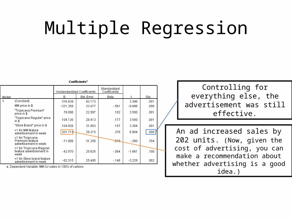
Controlling for everything else, the advertisement was still effective.
An ad increased sales by 202 units. (Now, given the cost of advertising, you can make a recommendation about whether advertising
is a good idea.)
Multiple Regression

Multiple Regression
Tropicana Ads do not influence Minute Maid sales, but Store Brand ads do.
What else can we learn?
It looks like ads generally decrease price sensitivities. (We would need to
test interactions to learn more about it)
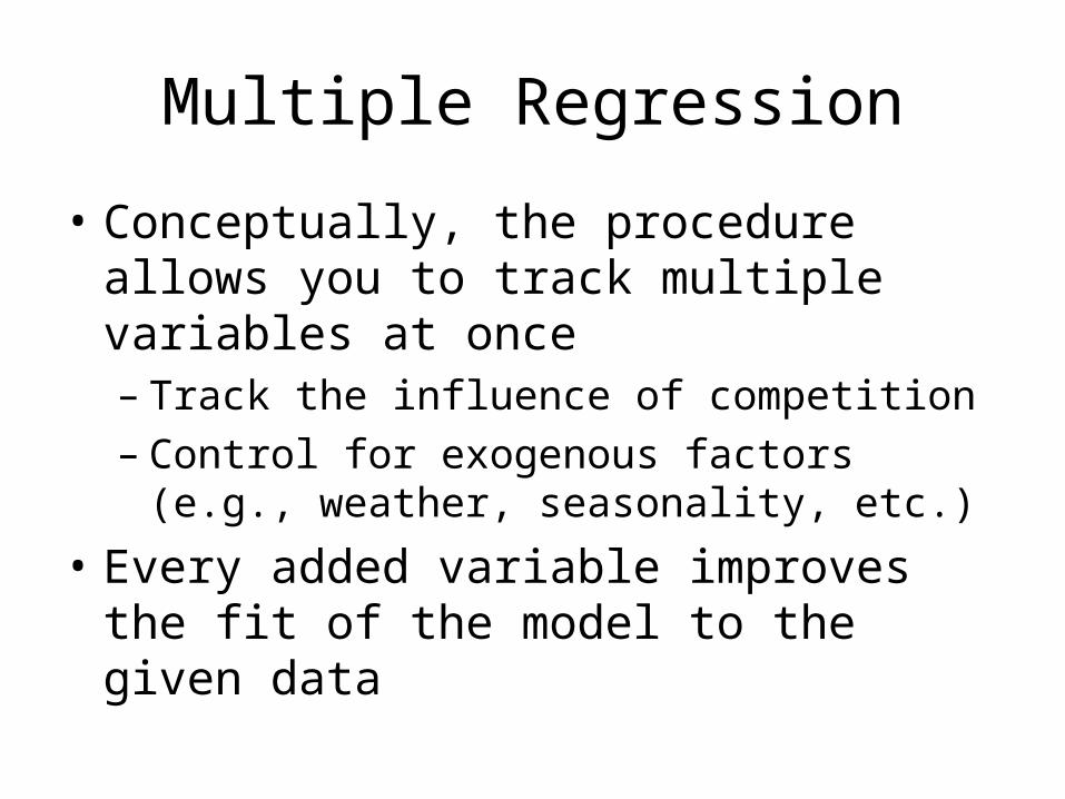
Multiple Regression
• Conceptually, the procedure allows you to track multiple variables at once– Track the influence of competition– Control for exogenous factors (e.g., weather,
seasonality, etc.)
• Every added variable improves the fit of the model to the given data

Multiple Regression
• Pitfalls:– That does not necessarily make it better at
predicting the future. You can “overfit” the data– Bad things happen when the predictors are
strongly related to each other– It intrinsically assumes that a linear model is a
pretty good approximation• It often is• But not always…

Key Points
• Regression not only helps make precise predictions, it can simultaneously account for multiple influences
• In so doing, it gets much closer to causal inferences (and good market researchers are after causal inferences)
• Nevertheless, regression is not a panacea, and should be used as a tool, not the only tool
• Nothing fixes poor research design
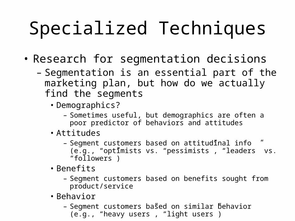
Specialized Techniques
• Research for segmentation decisions– Segmentation is an essential part of the marketing
plan, but how do we actually find the segments• Demographics?
– Sometimes useful, but demographics are often a poor predictor of behaviors and attitudes
• Attitudes– Segment customers based on attitudinal info (e.g., “optimists vs.
“pessimists”, “leaders” vs. “followers”)• Benefits
– Segment customers based on benefits sought from product/service
• Behavior– Segment customers based on similar behavior (e.g., “heavy
users”, “light users”)

Cluster Analysis• Cluster analysis is a
technique used to identify groups of ‘similar’ customers in a market (i.e., market segmentation).
• If some customers are very similar to one another but different from other (groups of) customers, cluster analysis can help you identify these (multiple) segments.
Price sensitivity
Bra
nd
Loya
lty
Cluster Analysis
• What is it actually doing?• The algorithm measures the “distance” between
every point and generates a solution which minimizes distances within a cluster and maximizes distances between clusters– Note that this language is very close to how you were
taught to think about the attributes of good segmentation
• What, exactly, is “distance”?– A rare literal example
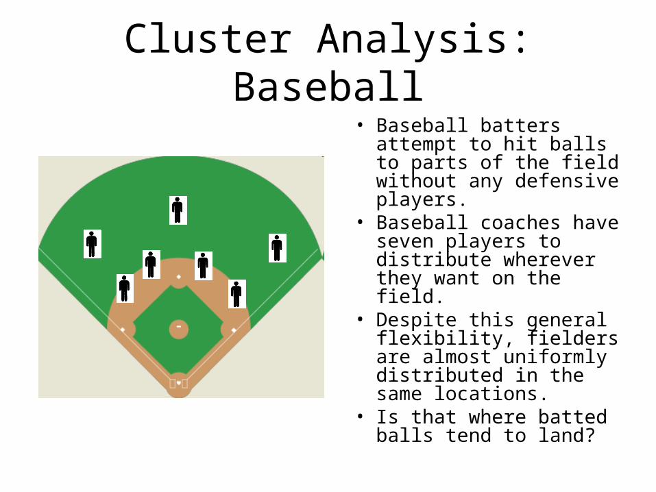
Cluster Analysis: Baseball• Baseball batters attempt
to hit balls to parts of the field without any defensive players.
• Baseball coaches have seven players to distribute wherever they want on the field.
• Despite this general flexibility, fielders are almost uniformly distributed in the same locations.
• Is that where batted balls tend to land?

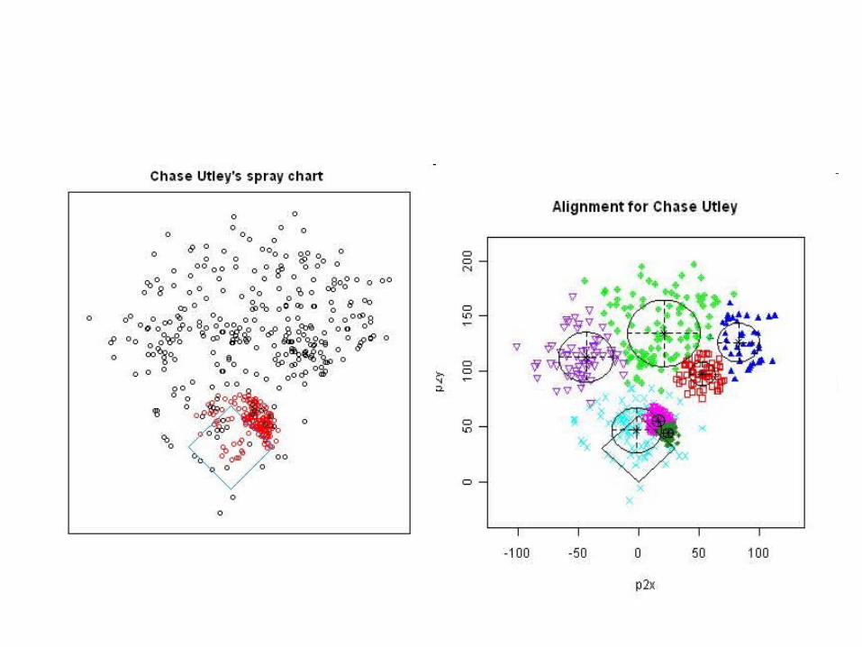
Chase Utley
Let’s look at clustering of batted balls for a single player.


Example: Shopping Attitudes
• V1: Shopping is fun• V2: Shopping is bad for your budget• V3: I combine shopping with eating out• V4: I try to get the best buys while shopping• V5: I don’t care about shopping• V6: You can save a lot of money by comparing
prices

Example: Shopping
• Cluster 1: _______________• Cluster 2: _______________• Cluster 3: _______________

Key Points
• Cluster Analysis allows us to simplify across respondents
• When used effectively, it can guide marketing strategy
• Nevertheless, it is by no means pure computational science. Identifying and labeling clusters requires some interpretation– This is a strength (in flexibility)– And a weakness

Clusters versus Factors
VV11 VV22 VV33 VV44 VV55 VV2020……....
Cluster Analysis
Factor Analysis
Data
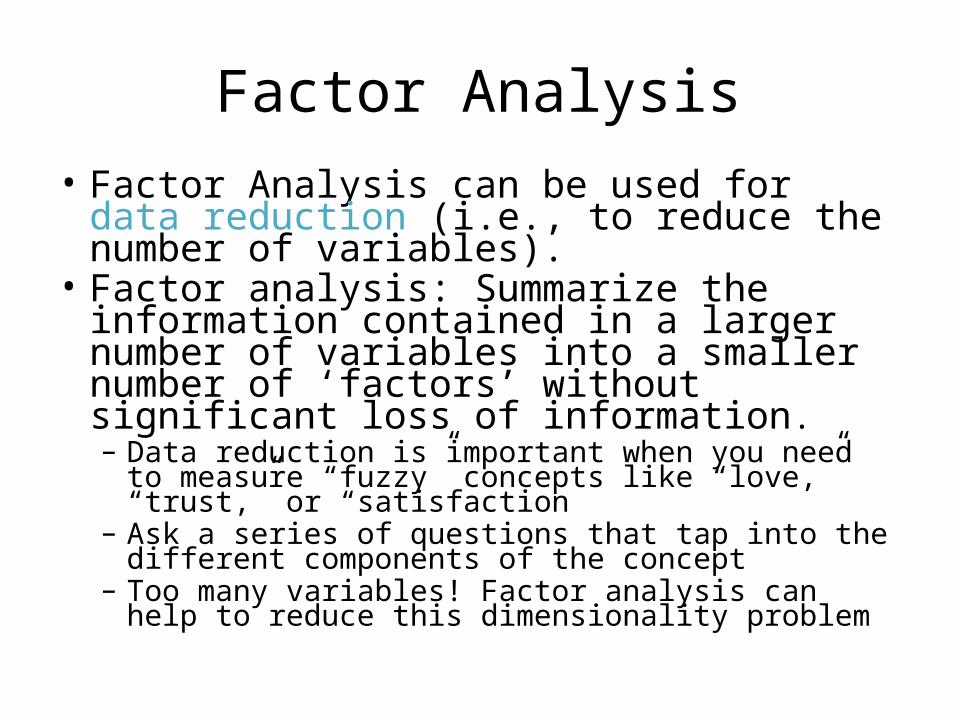
Factor Analysis• Factor Analysis can be used for data reduction
(i.e., to reduce the number of variables).• Factor analysis: Summarize the information
contained in a larger number of variables into a smaller number of ‘factors’ without significant loss of information.– Data reduction is important when you need to measure
“fuzzy” concepts like “love,” “trust,” or “satisfaction– Ask a series of questions that tap into the different
components of the concept– Too many variables! Factor analysis can help to reduce
this dimensionality problem

Factor Analysis: Intuition
• Factor analysis assumes that the correlation between a large number of variables is due to them all being dependent on the same small number of “factors”
• Example: Choice of movies– Suppose individuals choose movies based on two
main attributes:• Plot/story line (A1)• Production quality (A2)
– Each individual has a preference for A1 and A2

Example: Choice of Movies
A1 Weight A2 Weight
I can relate to the characters 0.81 -0.02
The movie is visually pleasing 0.07 0.92
Set and costume design are an important part of a movie
-0.13 0.85
Movie features major stars 0.09 0.16
Movie has first-rate special effects
-0.08 0.69
Engaging story-line 0.76 0.12I feel “transported” while watching
0.72 -0.18

Key Points
• Factor Analysis allows us to simplify across measures
• It helps hone in on large difficult concepts that a single item measures poorly
• It has a set of guidelines for interpretation and use (e.g., Eigenvalues > 1, KMO > .6), but it is only slightly less flexible than Cluster Analysis

Key Points• Market Research data is often extremely bulky and
complicated. We need tools simply to make it comprehensible– Cluster Analysis helps with complexity across consumers,
Factor Analysis helps with complexity across measures, Perceptual maps can helpfully present this information
• These analytic tools are well suited to basic strategic concerns– Identifying segments and matching them to preferences
and brand perceptions– In combination they are even better
• Use these tools carefully: Because there is room for interpretation, there is also room for clumsiness (or deceptiveness)
.
.
.
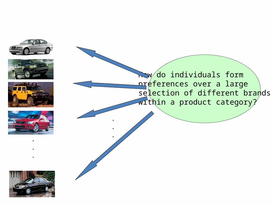
How do individuals form preferences over a large selection of different brandswithin a product category?
.
.
.

Engine Size HP Type #Doors Brand Price
2.5L 184 Sedan 4 BMW $27,800
4.0L 203 SUV 2 Ford $21,715
6.0L 316 SUV 4 Hummer $48,455
3.0L 215 Sedan 4 Lexus $29,435
2.4L 157 Sedan 4 Toyota $18,970
.
.
.
.
.
.
.
.
.
.
.
.
.
.
.
.
.
.
.
.
.
Think of different brandsas different combinations of attributes!

Attribute based approach
• Think of a product (a certain car) as a bundle of attributes.
• A consumer prefers a certain car, car A, to another, car B, because the attributes of car A are more appealing to the consumer than the attributes of car B.
• Suppose we assume that consumers form preferences over brands implicitly by forming preferences for the attributes of which the brands consists.
• So if we present certain lists of attributes the consumer can rank these.

Conjoint Analysis
• Conjoint Analysis: A technique that enables a researcher to estimate consumers’ valuations of different attributes– Allows us to understand how consumers make
trade-offs among attributes/characteristics of products and services
– How much are consumers willing to pay/give up to get/avoid different attributes?

Uses of Conjoint Analysis: New Products
• Estimate market share of brands that differ in attribute levels
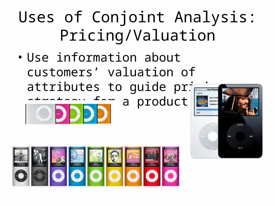
Uses of Conjoint Analysis: Pricing/Valuation
• Use information about customers’ valuation of attributes to guide pricing strategy for a product line

Uses of Conjoint Analysis: Brand Equity
• Brand name equity• How much is a brand really worth?
or

Assumption of Part-Worth’s
• Total utility = sum of utilities of each attribute
U( ) = u(motorola) + u(pink) + u($149) + u(flip format)+…
U( = ) u(motorola) + u(grey) + u($149) + u(flip format)+…
u(nokia) + u(black) + u($129) + u(candy bar format)+…U( = )

Example: New Job
$100 K $150 K
Salary
Location

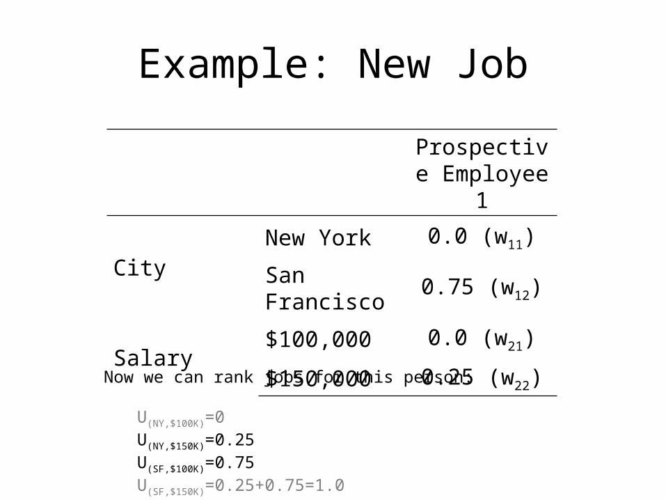
Example: New Job
Prospective Employee 1
CityNew York 0.0 (w11)
San Francisco 0.75 (w12)
Salary$100,000 0.0 (w21)
$150,000 0.25 (w22)
Now we can rank jobs for this person:
U(NY,$100K)=0U(NY,$150K)=0.25U(SF,$100K)=0.75U(SF,$150K)=0.25+0.75=1.0
Example: New Job
Prospective Employee 1
CityNew York 0.0 (w11)
San Francisco 0.75 (w12)
Salary$100,000 0.0 (w21)
$150,000 0.25 (w22)
Now we can rank jobs for this person:
U(NY,$100K)=0U(NY,$150K)=0.25U(SF,$100K)=0.75U(SF,$150K)=0.25+0.75=1.0

Example: New Job
Prospective Employee 1
Prospective Employee 2
CityNew York 0.0 (w11) 0.0 (w11)
San Francisco 0.75 (w12) 0.25 (w12)
Salary$100,000 0.0 (w21) 0 (w21)
$150,000 0.25 (w22) 0.75 (w22)
Now we can rank jobs for this person, and compare it to this person:
U(NY,$100K)=0U(NY,$150K)=0.25U(SF,$100K)=0.75U(SF,$150K)=0.25+0.75=1.0
U(NY,$100K)=0U(NY,$150K)=0.75U(SF,$100K)=0.25U(SF,$150K)=0.25+0.75=1.0

How do we get the part-worths?
• This is very nice but we don’t know consumers’ valuations of attributes…
• …and consumers probably don’t know their own valuations either!
• A solution: Force consumers to rank different bundles of attributes (i.e., “brands”)
A
B
C
D
E
F
A
C
E
F
B
D
1.
2.
3.
4.
5.
6.

Conjoint Analysis: Approaches• Traditional Conjoint: Have respondents directly rank or rate
a series of product profiles
• Discrete Choice Models (allows for non-choice)– Also called “Choice Based Conjoint”
• (from Sawtooth Software’s web-site: http://www.sawtoothsoftware.com/conjoint-analysis-software)
Conjoint ≈Consider Jointly

Standard Conjoint Analysis: Process
• Develop the set of attributes• Select the levels of each attribute• Obtain an evaluation (rating or ranking) of the product
profiles from respondents• Estimate the part-worths values for each level of each
attribute• Compute importance weights for each attribute
(normalized range)• Aggregation of results across consumers• Evaluate the tradeoffs among attributes• Market simulations• Evaluate accuracy of results

From Preference to Choice
• Conjoint model predicts utility, not choice• Utility is a continuous, relative measure of preference
for each alternative. Choice is a discrete outcome.• Need a rule to translate preferences to choices:
– First choice rule: Respondent chooses the profile with the highest predicted utility score
– Share of preference rule: Predictions of choice probabilities sum to 1 over the set of stimuli tested.
• First choice rule usually more appropriate for sporadic, non-routine purchases.
• However, both rules are ad hoc

Conjoint Pluses and Minuses• When to use CA:
– Can the product be seen as a bundle of attributes?• Avoid using CA for “image” products
– Are the respondents familiar with the category? • Avoid using CA for new-to-the-world products
– Must know relevant attributes (exploratory research)
• Warnings– CA will not indicate the absence of an important attribute – Attributes should be actionable to the firm– Interpolation between attribute levels ok – but do not
extend beyond the range selected

Key points
• Conjoint is a very popular and frequently useful tool for identifying the underlying utilities of consumers.
• It details the relative value of product attributes and guides product development and competitive pricing.
• Nevertheless, its application is deeply contingent on both the consumer and the product category.
Summary
• There are a number of useful statistical techniques that can help you understand your data– T-tests, crosstabs, and regression are basic tools
that can make comparisons and show relationships between marketing variables
– Cluster, factor, and conjoint analysis can help you understand your customers’ traits and preferences
• These tools are only effective if you have good research design to start