statistical sampling - icediced.cag.gov.in/wp-content/uploads/2016-17/ntp 01/iced_statistical... ·...
TRANSCRIPT

Statistical Sampling
Amit Bhola

2
Source : Internet
There are better ways of Sampling!

GENERALIZATION
3
Representative SampleFaithful Generalization

POPULATION
Population is ‘observations’ or ‘measurements’ of property
under consideration
DO not confuse this with No. Of Objects.(Objects may or may not be property under study)
Population
(a) ‘Height’ of Plants in a garden ‘Height’
(b) ‘No. of Plants’ in a garden ‘No. of plants’4

SAMPLE
A small part of a population
SAMPLING
Process of obtaining samples
STATISTICAL INFERENCE
Process of inferring facts about population from the results
found in samples
Aim of Sampling
5

POPULATION, SAMPLE & GENERALIZATION
SamplePopulation
6
Sampling Frame : Population accessible for sampling

SAMPLING METHODS & GENERALIZATION
7
PROBABILITY SAMPLING – Aim of Generalization
- Best effort is made to draw sample representative of
population
NON PROBABILITY SAMPLING – When?
- Generalization is not the aim
- Qualitative study, Pilot study, Demonstration of population trait
- Probability sampling is infeasible
- Inaccessible sampling frame, constraints of time, money, etc.
- Initial study to be followed by probability sampling
Focus

TYPES OF PROBABILITY SAMPLING
8
Probability Sampling
Simple Random
Systematic Random
Stratified Cluster

POPULATIONS & SAMPLE SIZE
EXAMPLE Population Sample
Estimate Avg. weight of college students by studying only 100
FiniteN
Finiten
Estimate Head or Tail of a coin tossInfinite Finite
n8
9

SAMPLING WITH REPLACEMENT
EXAMPLE Replacement
Estimate Avg. weight of college students by studying only 100 different students
No
Estimate how many bolts in a bin of 500 are defective by : picking one bolt checking it returning it …. (repeat say 20 times)
Yes
10
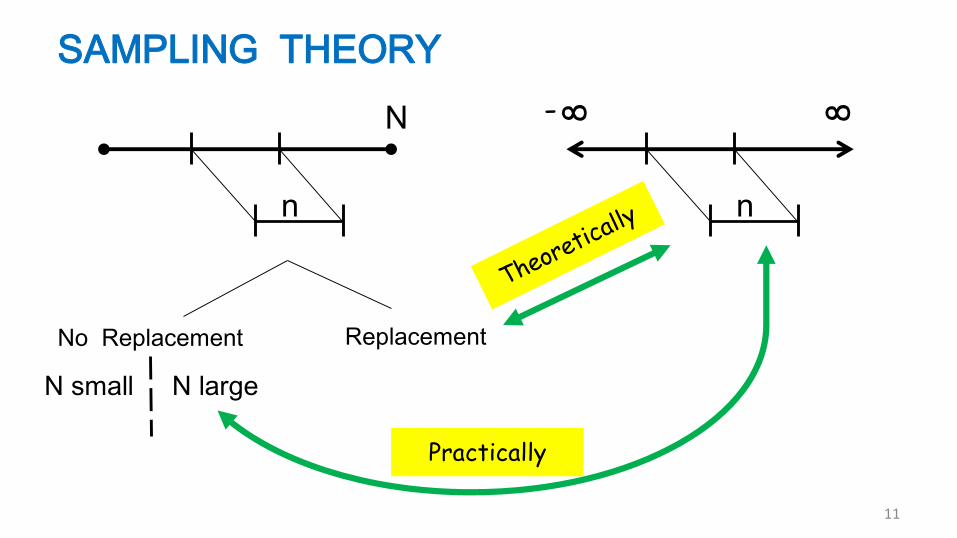
SAMPLING THEORY
N
n
88-
n
No Replacement Replacement
Practically
N small N large
11

RANDOMNESS
Being Random means being equally probable
A sample is random if there is no bias in selecting its n objects
Each object has equal chance of getting selected
To effectively represent a population, a sample should be
random
For getting a random sample of size n,
n random nos. should be obtained first
12

RANDOM NUMBER – MS EXCEL
14

BLINDING
15
Blinding is done to eliminate psychological bias
• Single Blinding : The participants (i.e. sample) are completely unaware of which group they are in and what intervention they are receiving until conclusion of the study.
• Double Blinding : Neither the participants nor the researcher knows to which group the participant belongs and what intervention the participant is receiving until the conclusion of study

SIMPLE RANDOM SAMPLING
STEP 1 : Obtain the approx size of population N
STEP 2 : Label the population items 1,2,… N
STEP 3 : Find n random nos.
STEP 4 : Select items labeled as nos. got in [3]
16

SIMPLE RANDOM SAMPLING
SYSTEMATIC RANDOM SAMPLING
N
Random Derived = pick every (N/n)th element
N
n sections
17
STEP 2 : Label the population items 1,2,… N

18
PROBLEM WITH SIMPLE / SYSTEMATIC
1. Need availability of complete list of population.
For a large population, this may not be
available!
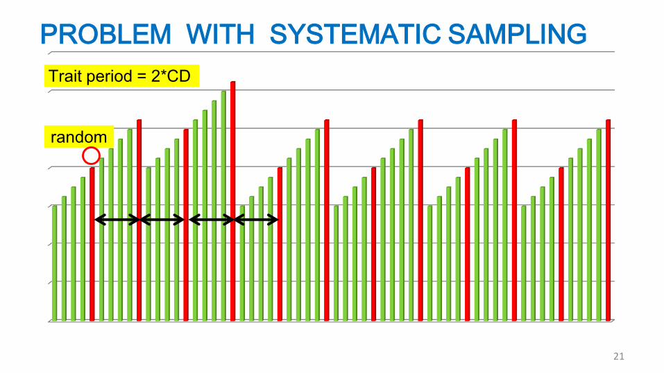
2. Although highly unlikely, Systematic sampling
carries risk of collecting a poor sample if (A)
there exist some periodic traits in the
population, and at the same time (B) The
period of the trait is a multiple of common
difference!
Sampling Frame Errors…

19
PROBLEM WITH SYSTEMATIC SAMPLING

20
PROBLEM WITH SYSTEMATIC SAMPLING
random
Trait period =CD
21
PROBLEM WITH SYSTEMATIC SAMPLING
random
Trait period = 2*CD

22
random
Trait period ≠ n*CD
DEALING PERIODICITY PROBLEM – 1

23
DEALING PERIODICITY PROBLEM – 2
random
Repeated sampling and combining two samples into one single sample
random
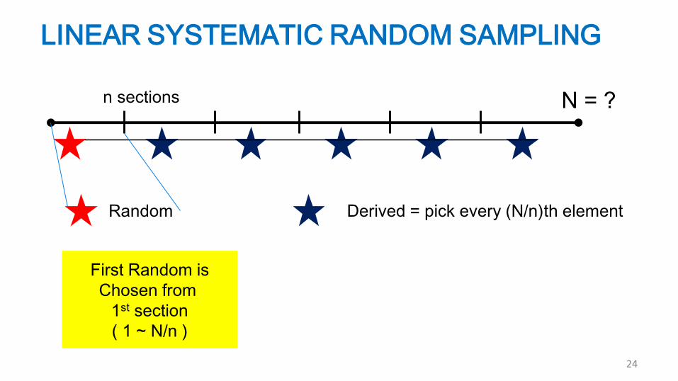
LINEAR SYSTEMATIC RANDOM SAMPLING
N = ?
Random Derived = pick every (N/n)th element
n sections
24
First Random is
Chosen from
1st section
( 1 ~ N/n )

CIRCULAR SYSTEMATIC RANDOM SAMPLING
26
Random
from
1 ~ N
Derived
till n samples
are obtained
Selection is
done with
continuing
counting at the
end of the list

TYPES OF PROBABILITY SAMPLING
27
Probability Sampling
Simple Random
Systematic Random
Linear
Repeated
Circular
Stratified Cluster

PROBLEM WITH SIMPLE / SYSTEMATIC
N
Random Derived
N
0% 10% 20% 30% 40% 50% 60% 70% 80% 90% 100%
E.g. :Mon Tue Wed Thu/Fri/Sat
28

STRATIFIED SAMPLING
N
0% 10% 20% 30% 40% 50% 60% 70% 80% 90% 100%
1. Divide N by category of Strata
Strata:
1. Divide N by category of Strata2. Select random samples from each Strata – in same ratio as that Strata
Mon Tue Wed Thu / Fri / Sat
29

STRATIFIED SAMPLING
30
Proportionate
=>
Representative of Population

STRATIFIED SAMPLING – ADVANTAGES
1. Ensures the presence of each subgroup within
the sample – better representation of population.
31
Especially useful for population with highly skewed strata eg. A:B::70:30
2. Permits analyses of within-stratum patterns and
separate reporting of the results for each stratum.

STRATIFIED SAMPLING – DIFFICULTIES
1. Requires information on the proportion of the
total population that belongs to each stratum.
32
2. More expensive, time-consuming, and
complicated than simple random sampling.
3. In order to calculate sampling estimates, at least
two elements must be taken in each stratum.

DISPROPORTIONATE STRATIFIED SAMPLING
33
Proportionate
=>
Representative of Population – Fine
But considering the cost of the sampling, studies other than the Generalization may separately
be performed at same time

DISPROPORTIONATE STRATIFIED SAMPLING
34
Dis-Proportionate
to
Represent all strata sufficiently
Example 1 :-Analysis of variation within
strata

DISPROPORTIONATE STRATIFIED SAMPLING
35
Dis-Proportionate
to
Represent all strata equally
Example 2 :-Analysis of variation among
strata

DISPROPORTIONATE STRATIFIED SAMPLING
36
Example 3 :-Optimization of Cost and/or
Precision
j 1/j 1200
18 0.055556 299.1371
10 0.1 538.4468
39 0.025641 138.0633
24 0.041667 224.3528
s 1200
4.3 189.7059
6.4 282.3529
9.4 414.7059
7.1 313.2353

TYPES OF STRATIFIED SAMPLING
37
Stratified Sampling
Proportionate Disproportionate
Within Strata analysis
Among Strata analysis
Optimization
Useful, but not as good
representative of
population
as Proportionate

CLUSTER SAMPLING
N
STEP 1 : Divide N into homogenous clusters
(Clusters : different from each other but same within)
Eg. Subjects , Districts , Offices-shops-showrooms38

CLUSTER SAMPLING
N
STEP 2 : Choose some clusters randomly
N
39

CLUSTER SAMPLING
N
STEP 3 : Recommendation but not must, select
whole of the selected clusters.N
40
(STEP 4) : Sampling within clusters may be done
Multi-Stage Sampling…

CLUSTER SAMPLING
N
N
Usual motive is to avoid the high cost of a geographical survey
Accuracy is not as good as Stratified, but in comparison to No Survey at all (due to high cost), it is better to do Cluster Sampling
E.g. TRPs , IQS . . .
41

Section 4
Section 5
Section 3
Section 2Section 1
CLUSTER SAMPLING
Source : Internet

CLUSTER SAMPLING vs. STRATIFIED
1. In stratified random sampling, all the strata of
the population are sampled while in cluster
sampling, only a part of clusters are sampled.
43
2 With stratified sampling, the best survey results
occur when elements within strata are internally
homogeneous. However, with cluster sampling,
the best results occur when elements within
clusters are internally heterogeneous.

CLUSTER SAMPLING – DISADVANTAGES
44
There is tendency for the clusters to display similar characteristics within themselves – especially so in case the clusters are regional
Statistically, it is the least precise compared to the
Simple, Systematic and Stratified sampling.

COMPARISON OF SAMPLING TECHNIQUES
EASYEASY
45

COMPARISON OF SAMPLING TECHNIQUES
>> ACCURATE
> ACCURATE
STRATA has to be known
46

COMPARISON OF SAMPLING TECHNIQUES
ECONOMICAL
QUICK
47

SELECTION OF SAMPLING TECHNIQUES
48

SELECTION OF SAMPLING TECHNIQUES
49
Merit based Sections
Gender based Sections

SELECTION OF SAMPLING TECHNIQUES
50
Merit based Sections
No particular criteria

CASE STUDY
THERE ARE AROUND 8,000 FIRMS ACROSS INDIA
PROVIDING A CAB SERVICE.
AN AUDIT IS TO BE PLANNED TO CHECK THE
CONFORMANCE OF TAX PAYMENTS.
51
ZONE OPERATORS
NORTH 4627
SOUTH 3423
CENTRAL 1488
EAST 891
WEST 2396
REVENUE NO. OF FIRMS
< 1 CRORE 4221
1 CR – 5 CR 3217
5 CR – 50 CR 770
50 CR – 250 CR 145
≥ 250 CR 13

CASE STUDY
52
ZONE OPERATORS
NORTH 4627
SOUTH 3423
CENTRAL 1488
EAST 891
WEST 2396
REVENUE NO. OF FIRMS
< 1 CRORE 4221
1 CR – 5 CR 3217
5 CR – 50 CR 770
50 CR – 250 CR 145
≥ 250 CR 13
HETROGENEOUS WITHIN
GEOGRAPHICAL
MUTUALLY EXCLUSIVE ?MUTUALLY EXCLUSIVE
HETROGENEOUS WITHIN
SKEWED PROPORTIONS
MUTUALLY EXCLUSIVE
PERIODIC TRAITS – NO
SKEWED PROPORTIONS
BUDGET ? / MULTI-STAGE ?
CLUSTERCLUSTER
SYSTEMATI
STRATIFIED STRATIFIED
SIMPLE SIMPLE

WHAT NEXT ?
53
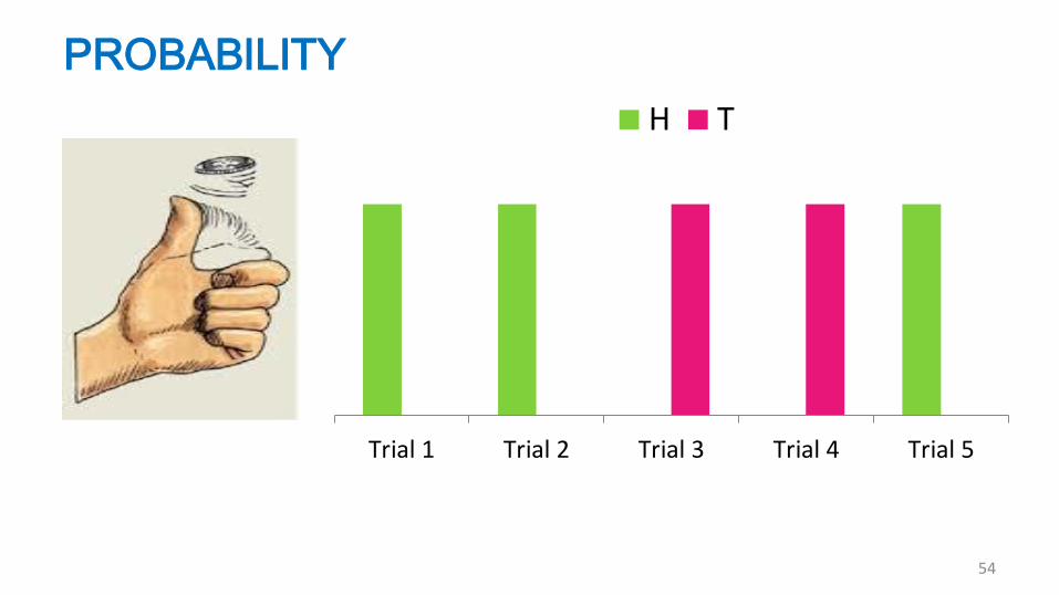
PROBABILITY
Trial 1 Trial 2 Trial 3 Trial 4 Trial 5
H T
54

PROBABILITY
Trial 1 Trial 2 Trial 3 Trial 4 Trial 5
H
T
0% 20% 40% 60% 80% 100%
p q = (1-p)
55

PROBABILITY
0
0.5
1
1.5
2
2.5
3
3.5
1 2 3 4 5 656

PROBABILITY
0
0.5
1
1.5
2
2.5
3
3.5
1 2 3 4 5 6
0% 20% 40% 60% 80% 100%
p1 p2 p3 p6
p4 p5
p1 + p2 + p3 + p4 + p5 + p6 = 1
57

PROBABILITY
Lucky No?
Pollution Level?
Height?
Person 1 2 3 4 5 6 7 8 9 10 11 12 … …
Response 5 73 46 20 4 97 5 38 13 51 … … …
The response / outcome possible is
NOT fixed / restricted.
Theoretically EVERY real no. has a
Non Zero Probability
58

PROBABILITY
Person 1 2 3 4 5 6 7 8 9 10 11 12 … …
Response 5 73 46 20 4 97 5 38 13 51 … … …
0 20 40 60 80 100 120
59

PROBABILITY
Person 1 2 3 4 5 6 7 8 9 10 11 12 … …
Response 5 73 46 20 4 97 5 38 13 51 … … …
0
1
2
3
4
5
6
0 20 40 60 80 100 120
HISTOGRAMS
TELL
PROBABILITY
60

WHAT NEXT ?
61

PROBABILITY
BINOMIAL MULTINOMIAL CONTINUOUS
p p1 p (R1) = f(R1)
q=1-p p2 ... p (R2) = f(R2) …
p+q=1 p1+p2+p3+...+pn= 1 ∑ p (all R) = 162

PROBABILITY
BINOMIAL MULTINOMIAL CONTINUOUS
p p1 p (R1)
q=1-p p2 ... p (R2) …
p+q=1 p1+p2+p3+...+pn= 1 ∑ p (all R) = 1
RARE
AND
COMPLEX
OUT
OF
SCOPE
Formulae 1 Formulae 2
63

HISTOGRAMS
0
2
4
6
8
10
12
14
16
-4 6 15 24 33 42 51 60 69 78 87 96
-8 - 1 1 - 10 10 - 19 19 - 28 28 - 37 37 - 46 46 - 55 55 - 64 64 - 73 73 - 82 82 - 91 91 - 100
64

PROBABILITY (DENSITY) FUNCTION
0
0.002
0.004
0.006
0.008
0.01
0.012
0.014
0.016
0
2
4
6
8
10
12
14
16
-4 6 15 24 33 42 51 60 69 78 87 96
-8 - 1 1 - 10 10 - 19 19 - 28 28 - 37 37 - 46 46 - 55 55 - 64 64 - 73 73 - 82 82 - 91 91 - 100
65

PROBABILITY FUNCTION
0
0.002
0.004
0.006
0.008
0.01
0.012
0.014
0.016
-8 1 10 19 28 37 46 55 64 73 82 91 100
66

CUMULATIVE DENSITY FUNCTION
0
0.002
0.004
0.006
0.008
0.01
0.012
0.014
0.016
-4-8 - 1
61 - 10
1510 - 19
2419 - 28
3328 - 37
4237 - 46
5146 - 55
6055 - 64
6964 - 73
7873 - 82
8782 - 91
9691 - 100
67

P.D.F. AS PROBABILITY INDICATOR
0
0.002
0.004
0.006
0.008
0.01
0.012
0.014
0.016
-4-8 - 1
61 - 10
1510 - 19
2419 - 28
3328 - 37
4237 - 46
5146 - 55
6055 - 64
6964 - 73
7873 - 82
8782 - 91
9691 - 100
More Area = More Probability
68

RANGE PROBABILITY FROM C.D.F.
0
0.002
0.004
0.006
0.008
0.01
0.012
0.014
0.016
-4-8 - 1
61 - 10
1510 - 19
2419 - 28
3328 - 37
4237 - 46
5146 - 55
6055 - 64
6964 - 73
7873 - 82
8782 - 91
9691 - 100
16%
84%
More Area = More Probability
69

RANGE PROBABILITY FROM C.D.F.
0
0.002
0.004
0.006
0.008
0.01
0.012
0.014
0.016
-4-8 - 1
61 - 10
1510 - 19
2419 - 28
3328 - 37
4237 - 46
5146 - 55
6055 - 64
6964 - 73
7873 - 82
8782 - 91
9691 - 100
60% 40%
70
It means 60% of values are likely to be < 51

RANGE PROBABILITY FROM C.D.F.
0
0.002
0.004
0.006
0.008
0.01
0.012
0.014
0.016
-4-8 - 1
61 - 10
1510 - 19
2419 - 28
3328 - 37
4237 - 46
5146 - 55
6055 - 64
6964 - 73
7873 - 82
8782 - 91
9691 - 100
87%
13%
71
It means 13% of values are likely to be > 78

RANGE PROBABILITY FROM C.D.F.
0
0.002
0.004
0.006
0.008
0.01
0.012
0.014
0.016
-4-8 -1
61 -10
1510 -19
2419 -28
3328 -37
4237 -46
5146 -55
6055 -64
6964 -73
7873 -82
8782 -91
9691 -100
87% - 16%= 71%
0
0.002
0.004
0.006
0.008
0.01
0.012
0.014
0.016
-4-8 -1
61 -10
1510 -19
2419 -28
3328 -37
4237 -46
5146 -55
6055 -64
6964 -73
7873 -82
8782 -91
9691 -100
87% - 60%
27%
72
It means 27% of values are likely to be between 51 and 78

NORMAL DISTRIBUTION
73
It means:-
Knowing μ and σ of a normally distributed variable, one can determine how much probable is it to lie between a range.
Most common

MEAN AND STANDARD DEVIATION
-0.005
0
0.005
0.01
0.015
0.02
0.025
-100 -90 -80 -70 -60 -50 -40 -30 -20 -10 0 10 20 30 40 50 60 70 80 90 100 110 120
μ = 40σ = 20
74

MEAN AND STANDARD DEVIATION
-0.005
0
0.005
0.01
0.015
0.02
0.025
-100 -90 -80 -70 -60 -50 -40 -30 -20 -10 0 10 20 30 40 50 60 70 80 90 100 110 120
-0.005
0
0.005
0.01
0.015
0.02
0.025
-100 -90 -80 -70 -60 -50 -40 -30 -20 -10 0 10 20 30 40 50 60 70 80 90 100 110 120
μ = 40σ = 20 vs. 30
More σ =>Wider range of values are more probable
σ = 20
σ = 30
75

AREA COVERED BETWEEN STD DEV
-0.005
0
0.005
0.01
0.015
0.02
0.025
-100 -90 -80 -70 -60 -50 -40 -30 -20 -10 0 10 20 30 40 50 60 70 80 90 100 110 120
68.27%
± σ
76
σ σ

-0.005
0
0.005
0.01
0.015
0.02
0.025
-100 -90 -80 -70 -60 -50 -40 -30 -20 -10 0 10 20 30 40 50 60 70 80 90 100 110 120
68.27%
AREA COVERED BETWEEN STD DEV
-0.005
0
0.005
0.01
0.015
0.02
0.025
-100 -90 -80 -70 -60 -50 -40 -30 -20 -10 0 10 20 30 40 50 60 70 80 90 100
68.27%
± σ
77
σ σ

AREA COVERED BETWEEN STD DEV
± σ
± 2σ
± 3σ± 1.96σ
78
1.96σ
1.96σ

AREA COVERED BETWEEN STD DEV
± σ
± 2σ
± 3σ± 2.58σ
79
2.58σ
2.58σ

SAMPLING THEORY
N
n
88-
n
No Replacement Replacement
Practically
N small N large
80

SAMPLING INFERENCE - MEAN
N
n
88-
n
μ
No Replacement Replacement
μ
μ* μ*
μ* = μ
Sample mean = Population mean
With some error81

SAMPLING INFERENCE - MEAN
82
I sampled
the ABC
tax
payments. I
conclude
that Avg.
tax as 1.2
MRs
How
much
sure are
you
about
your
inference
?

NORMAL DISTRIBUTION
83
It means:-
Knowing μ and σ of a normally distributed variable, one can determine how much probable is it to lie between a range.

SAMPLING INFERENCE – MEAN’s DISTRIBU.
N
n
88-
n
μ
No Replacement Replacement
μ
μ* μ*
84
Sampling Sampling 1 Sampling 2 Sampling 3 Sampling 4 …
Sample size n (say 100) n n n …
Sample mean μ*
μ1 μ2 μ3 μ4 …
μ* = sample mean is normally distributed N(μ*, σ*)
Even if
population is
not normal
!

NORMAL DISTRIBUTION
85
It means:-
Knowing μ and σ of a normally distributed variable, one can determine how much probable is it to lie between a range.

MARGIN OF ERROR
μ* ± 1.96σ*
This value is Margin of error at 95% confidence
σ* has special calculation86

MARGIN OF ERROR - CALCULATION
N
n
88-
n
σ
No Replacement Replacement
σ
σσ * = ----
√n
σ √(N-n)
σ * = ---------√n (N-1)
87

MARGIN OF ERROR - CALCULATION
N
n
88-
n
σ
No Replacement Replacement
σ
1.96 σE = ---------
√n
1.96σ √(N-n)
E = ---------√n (N-1)
88
μ* ± 1.96σ*
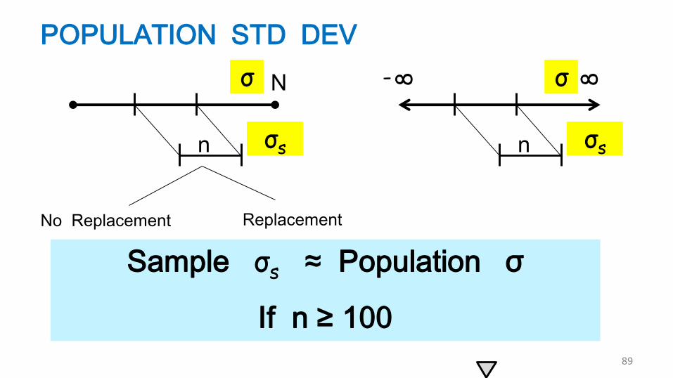
POPULATION STD DEV
N
n
88-
n
σ
No Replacement Replacement
σ
Sample σs ≈ Population σ
If n ≥ 100
σs σs
89

SAMPLING INFERENCE - MEAN
90
I sampled
240 firms
so n=240.
Also
240>100,
so ‘σ’ can be taken =
σs
1.96 σE = ---------
√n

SAMPLING INFERENCE - MEAN
91
In my
sample
σs came
out to be
0.8 MRs
σs ≈ σ ≈
0.8
1.96 σE = ---------
√n

SAMPLING INFERENCE - MEAN
92
So I can
say that
Margin of
Error = ± E
= ± 1.96*(0.8) /
(240^0.5)
≈ 0.1
1.96 σE = ---------
√n

SAMPLING INFERENCE - MEAN
93
Thus tax
Avg.
=1.2±E
=1.2±0.1
It lies b/w
1.1 to 1.3
MRs
μ* ± 1.96σ*
Always
?
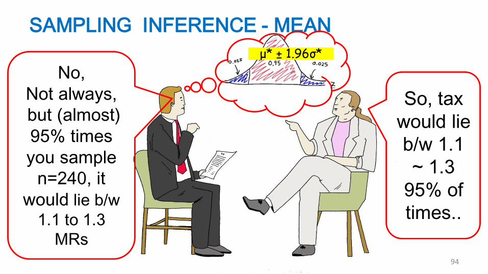
SAMPLING INFERENCE - MEAN
94
No,
Not always,
but (almost)
95% times
you sample
n=240, it
would lie b/w
1.1 to 1.3
MRs
μ* ± 1.96σ*
So, tax
would lie
b/w 1.1
~ 1.3
95% of
times..

SAMPLING INFERENCE - MEAN
95
Strictly
speaking -
No, Not the
tax.
We are
talking about
a particular
sample
statistic
here…
μ* ± 1.96σ*
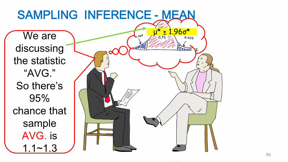
SAMPLING INFERENCE - MEAN
96
We are
discussing
the statistic
“AVG.”
So there’s
95%
chance that
sample
AVG. is
1.1~1.3
μ* ± 1.96σ*

SAMPLING INFERENCE - MEAN
97
If you ask me
99% confidence
level, my range
would be
E= ± 2.58*(0.8)
/ (240^0.5)
Avg.
=1.2 ± 0.133
b/w
1.067 to 1.333
μ* ± 2.58σ*
How to
further
reduce
the
margin
of Error
E ?

SAMPLE SIZE - CALCULATION
N
n
88-
n
σ
No Replacement Replacement
σ
98
21.96 σ
n = ---------
E
1.96 σE = ---------
√n
1.96σ √(N-n)
E = ---------√n (N-1)
Calculate n using the desired E

SAMPLE SIZE - CALCULATION
N
n
88-
n
σ
No Replacement Replacement
σ
21.96 σ
n = ---------E
1.96σ √(N-n)
E = ---------√n (N-1)
N large
99

MARGIN OF ERROR - BINOMIAL
N
n
88-
n
p
No Replacement Replacement
p
√pqσ* = -----
√n
√pq (N-n)σ* = ------------
√n (N-1)
100

MARGIN OF ERROR - BINOMIAL
N
n
88-
n
p
No Replacement Replacement
p
1.96 √pqE = ----------
√n
1.96 √pq (N-n)
E= ----------------√n (N-1)
101

SAMPLE SIZE - BINOMIAL
N
n
88-
n
p
No Replacement Replacement
p
1.96 √pqE = ----------
√n
1.96 √pq (N-n)
E= ----------------√n (N-1)
102
21.96 √pq
n = ---------
E
Calculate n using the desired E

SAMPLE SIZE - BINOMIAL
88-
n
p
103
21.96 √pq
n = ---------
E
p & q are expected
ideal population
proportions here
When not known
beforehand, assumed
p = q = 0.5
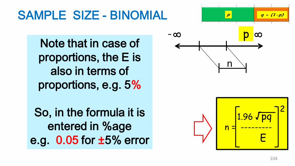
SAMPLE SIZE - BINOMIAL
88-
n
p
104
21.96 √pq
n = ---------
E
Note that in case of
proportions, the E is
also in terms of
proportions, e.g. 5%
So, in the formula it is
entered in %age
e.g. 0.05 for ±5% error

SAMPLE SIZE - BINOMIAL
88-
n
p
105
n = 384
So, example
calculation for E=5%
and unknown p & q,
& 95% confidence
21.96 √0.5*0.5
n = --------------
0.05
21.96 √0.5*0.5
n = --------------
E

CAUTION ! APPLICABILITY
106
μ* ± 1.96σ*
106
Sampling Sampling 1 Sampling 2 Sampling 3 Sampling 4 …
Sample size n (say 100) n n n …
Sample mean μ*
μ1 μ2 μ3 μ4 …
μ* = sample mean is normally distributed N(μ*, σ*)
The Formulas of Margin of Error E studied are valid only for the sampling statistic = AVERAGE μ* And not for other sampling statistics like STD DEV. etc.

REPORTING STATISTICS
PARAMETER MENTIONED IN SAMPLING REPORT
CHECK
Basic Assumptions about Population
Sampling Technique used
Sample Size
Sampling Inference (outcome, eg. μ)
Margin of Error (± E)
Confidence Level (eg. 95%)
WHAT NEXT ?
108

HISTOGRAMS – BIN SIZE
39.185 39.147 39.229 39.205 39.246
39.257 39.304 39.278 39 39.17
39.243 39.309 39.264 39.315 39.203
39.287 39.185 39.276 39.232 39.387
39.253 39.251 39.345 39.353 39.255
39.292 39.251 39.177 39.28 39.391
39.245 39.197 39.148 39.293 39.255
39.18 39.072 39.317 39.177 39.119
39.269 39.071 39.236 39.351 39.294
39.271 39.27 39.39 39.12 39.401
38.58 0
38.75 0
38.92 0
39.08 3
39.25 19
39.42 28
0
10
20
30
38.58 38.75 38.92 39.08 39.25 39.42
109

HISTOGRAMS – BIN SIZE
38.58 0
38.75 0
38.92 0
39.08 3
39.25 19
39.42 28
0
5
10
15
20
25
30
38.
58
38.
75
38.
92
39.
08
39.
25
39.
42
38.58 0
38.72 0
38.86 0
39.00 0
39.14 5
39.28 28
39.42 17
38.58 0
38.69 0
38.79 0
38.90 0
39.00 0
39.10 3
39.21 13
39.31 25
39.42 9
38.58 0
38.67 0
38.75 0
38.83 0
38.92 0
39.00 0
39.08 3
39.17 4
39.25 15
39.33 21
39.42 7
110

HISTOGRAMS – BIN SIZE
0
10
20
303
8.5
8
38.
75
38.
92
39.
08
39.
25
39.
42
0
10
20
30
38.
58
38.
72
38.
86
39.
00
39.
14
39.
28
39.
42
05
1015202530
0
5
10
15
20
25
Thumb Rule
Bin Size = √n
111

HISTOGRAMS – FIT NORMAL DISTRIBUTION
-1
0
1
2
3
4
5
0
5
10
15
20
25
30
38.58 38.75 38.92 39.08 39.25 39.42
Find
Mean & Std Dev.
112

WHAT NEXT ?
113

MISUSE OF STATISTICS – CASE STUDY 1
114
I II III IV
x y x y x y x y
10 8.04 10 9.14 10 7.46 8 6.58
8 6.95 8 8.14 8 6.77 8 5.76
13 7.58 13 8.74 13 12.74 8 7.71
9 8.81 9 8.77 9 7.11 8 8.84
11 8.33 11 9.26 11 7.81 8 8.47
14 9.96 14 8.1 14 8.84 8 7.04
6 7.24 6 6.13 6 6.08 8 5.25
4 4.26 4 3.1 4 5.39 19 12.5
12 10.84 12 9.13 12 8.15 8 5.56
7 4.82 7 7.26 7 6.42 8 7.91
5 5.68 5 4.74 5 5.73 8 6.89
Mean 9 7.500909 9 7.500909 9 7.5 9 7.500909
Std Dev 3.316625 2.031568 3.316625 2.031657 3.316625 2.030424 3.316625 2.030579
Covar(x,y) 5.000909091 5 4.997272727 4.999090909

MISUSE OF STATISTICS – CASE STUDY 1
115
y = 0.5001x + 3.0001
0
5
10
15
0 5 10 15
y = 0.5x + 3.0009
0
5
10
15
0 5 10 15
y = 0.4997x + 3.0025
0
5
10
15
0 5 10 15
y = 0.4999x + 3.0017
0
5
10
15
0 5 10 15 20

WHAT NEXT ?
116

MISUSE OF STATISTICS – CASE STUDY 2
117
A B C D E F G H
Jan 8 2 7 9 8 2 8 5
Feb 2 3 7 4 9 1 9 9
Mar 8 3 8 8 1 8 2 3
Apr 9 3 9 3 7 2 9 6
May 3 4 8 7 2 2 9 8
Jun 9 2 8 3 9 2 9 7
Jul 2 3 9 2 3 1 8 2
Aug 8 3 7 2 8 9 3 6
Sep 3 4 8 4 6 2 9 7
Oct 2 2 8 2 7 1 9 7
Nov 9 2 9 5 8 1 8 6
Dec 2 3 7 3 8 2 9 4
A B C D E F G H
Average 5.42 2.83 7.92 4.33 6.33 2.75 7.67 5.83
0
5
10
Jan Feb Mar Apr May Jun Jul Aug Sep Oct Nov Dec
F
B

MISUSE OF STATISTICS – CASE STUDY 3
118
EXCELLENTVERY
GOODGOOD AVERAGE POOR
+ + + 0 - - -

Thanks
119