Statistical network models for systemic risk

Fabrizio Lillo

Scuola Normale Superiore

Pisa, Italy

October 22, 2015

1 / 51

Systemic risk

I Financial systemic risk is mediated by a set of interconnectednetworks

I Questions:I Which data are necessary to assess systemic risk?I What is the role of network structure and how do networks change in

response to exceptional events?

I (At least) two channels of systemic risk propagationI Common exposures and fire sale spilloversI Illiquidity cascades in the interbank network

2 / 51

Bipartite banks-assets network

Di Gangi, D., Lillo, F., and Pirino, D. (2015).Assessing Systemic Risk Due to Fire Sales Spillover Through MaximumEntropy Network Reconstruction.Available at SSRN: http://dx.doi.org/10.2139/ssrn.2639178

3 / 51

Fire sale spillovers

I Fire sales spillovers due to assets’ illiquidity and common portfolioholdings are definitely one of the main drivers of systemic risk.

I Shared investments create a significant overlap of portfolios betweencouples of financial institutions.

I Fire sales move prices due to the finite liquidity of assets and tomarket impact.

I Finally, leverage management amplifies such feedbacks.

4 / 51

Systemic Risk

1

2

3

...

N

1

2

3

...

K

Investors Assets

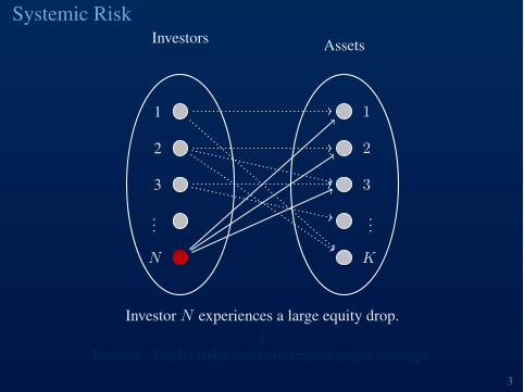
Financially interconnected world: assets are shared among financialinstitutions.

2

Systemic Risk

1

2

3

...

N

1

2

3

...

K

Investors Assets

Investor N experiences a large equity drop.ó

Investor N sells risky assets to restore target leverage.

3

Systemic Risk

1

2

3

...

N

1

2

3

...

K

Investors Assets

Investor N experiences a large equity drop.ó

Investor N sells risky assets to restore target leverage.

4

Systemic Risk

1

2

3

...

N

1

2

3

...

K

Investors Assets

Value of assets reduced proportionally to their illiquidity.

5

Systemic Risk

1

2

3

...

N

1

2

3

...

K

Investors Assets

Portfolios’overlap ñ total asset value of other investors is reduced.

6

Systemic Risk

1

2

3

...

N

1

2

3

...

K

Investors Assets

Further drop of value and spreading of the distress to new ones.

7

Fire sale spillovers

I Duarte, F. and T. M. Eisenbach (2013). Fire-sale spillovers andsystemic risk. Federal Reserve Bank of New York Sta↵ Reports,No.645

I Cont, R. and L. Wagalath (2014). Fire sales forensics: measuringendogenous risk.

I Caccioli, F., M. Shrestha, C. Moore, and J. D. Farmer (2014).Stability analysis of financial contagion due to overlapping portfolios.

I Greenwood, R., A. Landier, and D. Thesmar (2015). Vulnerablebanks.

I Our modeling contributionI Fire sales and target leveraging can generate a non stationary

dynamics for returns (Corsi, Marmi, Lillo, Operation Research 2015)I Di↵erent forms of expectations of investors can generate chaotic

dynamics (Mazzarisi, Marmi and Lillo, in progress)I The possibility of fire sales risk should be included in the

computation of the haircut of repos (Pirino and Lillo Journal ofEcon. Dyn. Control, 2015)

5 / 51

Questions and our contribution

I How is it possible to monitor, identify, and possibly forecast theoccurrence of fire sales spillover?

I Which kind of data is necessary? Is it possible to use publiclyavailable data? Do systemic risk metric truly depends on thedetailed portfolio composition of financial institutions?

I Our contributions:I Econometric approach (Corsi, F., F. Lillo, and D. Pirino (2015).

Measuring flight-to-quality with Granger-causality tail risk networks.Available at SSRN: http://ssrn.com/abstract=2576078.)

IMaximum Entropy approach (Di Gangi, D., Lillo, F., and Pirino, D.(2015). Assessing Systemic Risk Due to Fire Sales Spillover ThroughMaximum Entropy Network Reconstruction. Available at SSRN:http://dx.doi.org/10.2139/ssrn.2639178)

6 / 51

Systemic risk metrics: Vulnerability and Systemicness

I Metrics of systemic risk of individual banks and in aggregateintroduced by Greenwood et al. (2015)

I A system composed by N banks and K asset classes.

I Matrix X of portfolio holdings, whose element Xn,k is thedollar-amount of k-type assets detained by bank n.

I Matrix of portfolio weights is

Wn,k (X) =Xn,kPK

k0=1

Xn,k0.

I Discretization of Xn,k , in such a way that the matrix X belongs tothe space NN⇥K of N ⇥ K integer valued matrices

7 / 51

The bipartite network

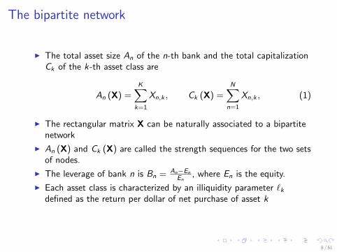
I The total asset size An of the n-th bank and the total capitalizationCk of the k-th asset class are

An (X) =KX

k=1

Xn,k , Ck (X) =NX

n=1

Xn,k , (1)

I The rectangular matrix X can be naturally associated to a bipartitenetwork

I An (X) and Ck (X) are called the strength sequences for the two setsof nodes.

I The leverage of bank n is Bn = An�En

En, where En is the equity.

I Each asset class is characterized by an illiquidity parameter `kdefined as the return per dollar of net purchase of asset k

8 / 51

The Greenwood et al (2015) metrics for systemic risk dueto fire sales

Given an asset shock described by the K dimensional vectorF1

= �" = (�"1

, ...,�"K ), Greenwood et al. define

IAggregate vulnerability AV as [...] the percentage of aggregatebank equity that would be wiped out by bank deleveraging if therewas a shock [...] to asset returns.

IBank systemicness Sn as the contribution of bank n to aggregatevulnerability.

IBank’s indirect vulnerability IVn [...] as the impact of the shockon its equity through the deleveraging of other banks.

9 / 51

Derivation of metrics for systemic risk

I Banks returns given asset returns, R1

= WF1

,

I Banks sell asset to return to leverage targets, then asset change ofbanks is A

1

BR1

I Proportional rebalancing of banks, asset purchase by all banks is� = W 0A

1

BR1

I Fire sales generate (linear) price impact, F2

= L�

I E↵ect on banks of fire sales, R2

= WF2

= WL� = (WLW 0BA1

)R1

I Aggregate vulnerability

AV =10A

1

·WLW 0BA1

WF1

E1

(2)

I Bank systemicness, i.e. its contribution to AV is

Sn =10A

1

·WLW 0BA1

�n�0nWF1

E1

(3)

10 / 51

SummaryI

Sn = �nAn

EBn rn, (4)

where E is the total equity, E =PN

n=1

En, rn is the n-th element ofthe vector r = W ", i.e. the portfolio return of bank n due to theshock ", and

�n =KX

k=1

NX

m=1

Am Wm,k

!`k Wn,k .

I

AV =NX

n=1

Sn. (5)

I

IVn = (1 + Bn)KX

k=1

`k Wn,k

NX

n0=1

Wn0,k An0 Bn0 rn0 . (6)

I As in Duarte and Eisenbach (2013) we assume that ✏k = 1% for allk = 1, ...,K , which in turns implies that rn = 1%. Note that if allassets are shocked by the same amount our results do not depend onit.

11 / 51

Network reconstruction and network statistical model

I The assessment of systemic risk according to Greenwood et al(2015) requires the knowledge of the portfolio holdings of all thefinancial institutions. This information might be not available or beavailable at a very low frequency (or with a time delay).

I Is it possible to assess systemic risk due to fire sales spilloverwithout a detailed knowledge of the portfolio holdings? Is thisinformation truly necessary?

I To answer this question, we will use two related approaches:I The Cross-Entropy ApproachI The Maximum Entropy Approach

12 / 51

The Cross-Entropy approachI Select an a priori guess for the matrix X and then to find its closest

matrix subject to some constraints.

I The guess might be based on partial knowledge of the matrix or onsome economic intuition.

I As a measure of distance to be minimized one uses theKullback-Leibler divergence.

I

minX

NX

n=1

KX

k=1

Xn,k log

Xn,k

eXn,k

!

s.t.NX

n=1

Xn,k = A?n, n = 1, ...,N,

KX

k=1

Xn,k = C?k , k = 1, ...,K ,

Xn,k � 0,

(7)

where eXn,k are the entries of the guess matrix.

13 / 51

Example of Cross-Entropy: the interbank market

I Many central banks do not require banks to report each credit ordebt position, but only the aggregated assets and liabilities

I In network terms this means that one knows only the node’s in- andout- strenght but not the degree, the adjacency matrix, and theweights of the individual links

I Assessing systemic risk through interbank market requires theknowledge of the interbank network. Is it possible to infer thestructure of the interbank network form balance sheet data?

I Distance can be quantified by the Kullback-Leibler divergence

DKL(~L, ~Q) =X

↵

L↵ lnL↵Q↵

(8)

I How does maximum entropy perform when we can benchmark itwith observable interbank networks?

14 / 51

Pitfalls of cross-entropy approach for interbank markets

”To sum up, the evidence suggests that, in most cases, ME tends tounderrate the impact of financial contagion. On the contrary, for highloss rates, ME may imply an overvaluation in the severity of contagion.”(Mistrulli, JBF 2011)

This results is due to the high sparsity of the interbank network. Entropymethods tend to spread the strength across a very large number of links(dense network).

15 / 51

Cross-Entropy approach for fire sales spillover: the dataset

I We test this approach on the dataset of US Commercial Banks andSavings and Loans Associations in the period 2001-2013.

I The quarterly balance sheet data are available by the Call Reports ofthe Federal Financial Institutions Examination Council.

I 55 quarters including several financial turmoil periods

I 6, 500� 9, 000 banks

I 20 asset classes (as in Duarte and Eisenbach (2013))

I The network is dense (50% of non-zero entries) but not fullyconnected.

16 / 51

Bank size distribution

102

104

106

108

10−15

10−14

10−13

10−12

10−11

10−10

10−9

10−8

10−7

Size

De

ns

ity

Figure: Plot, on a log-log scale, the kernel density of bank sizes (defined astotal assets in unit of 103$) computed using all records pooled across the entiretime span.

17 / 51

Leverage distribution

0 5 10 15 20 25 30 35 40 45 500

0.02

0.04

0.06

0.08

0.1

0.12

0.14

0.16

Leverage

De

ns

ity

Figure: Kernel density of the bank leverages computed using all records pooledacross the entire time span. For the sake of visualization, we put a cut-o↵ of 50on the maximum leverage allowed, although leverages of more than 150 are(rarely) observed.

18 / 51

Relation between size and leverage

104

105

106

107

108

10−3

10−2

10−1

100

101

102

103

Mean Size

Me

an

d a

nd

Std

. o

f L

ev

era

ge

Mean

Standard Deviation

Figure: Relation between leverage and size. The procedure adopted to drawthe plot is the following: all records of bank size are sorted from the smallest tothe largest one and a rolling window of 1000 records is moved, with anincremental shift of 10 records, from the first to the last. In each window wecompute the mean leverage (black continuous line) and the standard deviationof leverage (red dotted line) of banks that fall in the window.

19 / 51

The choice of a prior: the CAPM

I Similarly to Mistrulli (2011) for the interbank network, we choose aprior consistent with the capital asset pricing model (CAPM).

I Investors choose their portfolio in such a way that each weight on astock is the fraction of that stock’s market value relative to the totalmarket value of all stocks.

I This implies

X CAPM

n,k =C?k A

?n

L⇤. (9)

where L? =PK

k=1

C?k is the total market value of all stocks.

I In our case eXn,k = X CAPM

n,k .

I Note that the ”reconstructed” network is di↵erent from the real one(for example the former is fully connected but the latter not).

I If other information are available they can be set as constraints ofthe optimization.

20 / 51

Ag

gre

ga

te V

uln

era

bil

ity

(%

)

Q1−

2001

Q3−

2001

Q1−

2002

Q3−

2002

Q1−

2003

Q3−

2003

Q1−

2004

Q3−

2004

Q1−

2005

Q3−

2005

Q1−

2006

Q3−

2006

Q1−

2007

Q3−

2007

Q1−

2008

Q3−

2008

Q1−

2009

Q3−

2009

Q1−

2010

Q3−

2010

Q1−

2011

Q3−

2011

Q1−

2012

Q3−

2012

Q1−

2013

Q3−

2013

Q1−

2014

Q3−

2014

10

12

14

16

18

20

22

True

CAPM

Figure: This figure reports as a black continuous line the aggregatedvulnerability, as defined by equation (5), computed on the matrix X ?

n,k ofportfolio holdings as provided by the FFIEC dataset of US commercial bankholdings. The red dotted line is the aggregated vulnerability computed on theCAPM-implied matrix defined in equation (9) and that requires only theinformation on the strength sequences A?

n and C?k .

21 / 51

Comments

I At an aggregate level, the knowledge of the portfolio holdings isunnecessary. The size of banks and asset classes, plus the CAPMassumption, allow to reconstruct quite faithfully the aggregatevulnerability of the banking system.

I The Cross-Entropy method returns a single matrix.

I However for statistical purposes (e.g. hypothesis testing) it isnecessary to have as an output a probability distribution of thenetworks.

I This might be useful to assess confidence intervals to the metrics, toidentify statistically significant changes in a metric, to identifynetwork features which are not consistent with the null model.

I To this end we make use of the Maximum Entropy Principle

22 / 51

Network Statistical Models

I A network (statistical) model is defined by a set X of graphs that iscalled ensemble and a probability mass function P# indexed by avector of model parameters #. In formula it is expressed as thetriplet

{ P#,X ,# 2 ⌅ } ,I The probability mass function P# [X] is a function defined on X

with value in [0, 1]P# : X ! [0, 1] ,

and such thatP

X2X P# (X) = 1.

I For an arbitrary (regular enough) network function F : X ! Rdefined on the set X , the expected value of F on the ensemble X isdefined as

EX [F ] =X

X2XF (X) P# [X] .

23 / 51

The Maximum Entropy Principle

In the general setting, the probability mass function P# is the one thatmaximizes the Shannon’s entropy

S = �X

X2XP# [X] log (P# [X])

with the normalization constraintX

X2XP# [X] = 1,

and further additional constraints to define a specific ensemble.

The additional constraints can be such that:

I only the graphs which satisfy the constraints are allowed(microcanonical ensemble).

I all the graphs are allowed and the constraints are satisfied onaverage (canonical or grand-canonical ensemble).

24 / 51

Some literature

Growing attention toward Maximum Entropy in (financial) networkmodeling, mostly in the unipartite case.

I Park, J. and M. E. J. Newman (2004). Statistical mechanics ofnetworks.

I Mistrulli, P. E. (2011). Assessing financial contagion in theinterbank market: Maximum entropy versus observed interbanklending patterns.

I Squartini, T., I. van Lelyveld, and D. Garlaschelli (2013).Early-warning signals of topological collapse in interbank networks.

I Mastrandrea, R., T. Squartini, G. Fagiolo, and D. Garlaschelli(2014). Enhanced reconstruction of weighted networks fromstrengths and degrees.

I Anand, K., B. Craig, and G. von Peter (2015). Filling in the blanks:network structure and interbank contagion.

I Bargigli, L., G. di Iasio, L. Infante, F. Lillo, and F. Pierobon (2015).The multiplex structure of interbank networks.

25 / 51

Bipartite Weighted Configuration Model

The additional constraints are the (average) strength of each node (i.e.the bank and asset size).

maxP#

�X

X2XP# [X] log (P# [X])

s.t.X

X2XP# [X] = 1

EX [An] = A?n, n = 1, ...,N,

EX [Ck ] = C?k , k = 1, ...,K .

26 / 51

The Lagrangian associated to the problem is written as

L = S (P# [X]) + ↵

1�

X

X2XP# (X)

!+

NX

n=1

�n

A?n �

X

X2XP# (X)An (X)

!+

+KX

k=1

⌘k

C?k �

X

X2XP# (X)Ck (X)

!, (10)

whose extremal point is

P# (X) =e�H#(X)

Z#,

where H# (X) is the a function H# : X ! R defined as

H# (X) =NX

n=1

�n An (X) +KX

k=1

⌘k Ck (X) ,

and Z# is a normalizing factor given by

Z# =X

X2Xe�H#(X) =

NY

n=1

KY

k=1

('n ⇠k)Xn,k (1� 'n ⇠k) .

where 'n = e��n and ⇠k = e�⌘k .27 / 51

The value of the Lagrange multipliers are determined by imposing thatthe expected value of An (X) and Ck (X) on the ensemble X are equal to,respectively, A?

n and C?k . Note that the partition function Z# in (11) is

such that

@ log (Z#)

@�n= �EX [An]

@ log (Z#)

@⌘k= �EX [Ck ]

Therefore the Lagrange multipliers are determined by numerically solvingthe non-linear system of equations

8><

>:

PKk=1

'n ⇠k1�'n ⇠k

= A?n, n = 1, ..., n,

PNn=1

'n ⇠k1�'n ⇠k

= C?k , k = 1, ...,K .

(11)

28 / 51

Bipartite Enhanced Configuration ModelWe consider another (richer) statistical ensemble obtained by imposingboth the mean value of strengths (as in BIPWCM) and the mean valueof degrees, that is the number of edges incident in each vertex.

maxP#

�X

X2XP# [X] log (P# [X])

s.t.X

X2XP# [X] = 1

EX [An] = A?n,

EX [Drow

n ] = Drow

?

n , n = 1, ...,N,

EX [Ck ] = C?k ,

EX⇥Dcol

k

⇤= Dcol

?

k , k = 1, ...,K ,

(12)

where Drow

n and Dcol

k are, respectively, the row and the column degreesequences

Even if this information might be not available, we consider it to see ifadditional information (the degrees) increases the performance of theinference.

29 / 51

Maximum Entropy Capital Asset Pricing Model

Given the peculiar role of the CAPM in reproducing the aggregatevulnerability, we introduce a new ensemble where each link has anaverage weight given by the CAPM, i.e.

maxP#

�X

X2XP# [X] log (P# [X])

s.t.X

X2XP# [X] = 1

EX [Xn,k ] = X CAPM

n,k , n = 1, ...,N, k = 1, ...,K .

(13)

Note that only the information on the strength is needed.

We prove that

P# [X] =NY

n=1

KY

k=1

X CAPM

n,k

1 + X CAPM

n,k

!Xn,k

1

1 + X CAPM

n,k

, (14)

30 / 51

Summary of methods

I BIPWCM estimator: only the information on the strength sequencesis used

I BIPECM estimator: the information on the strength and degreesequences is used

I MECAPM estimator: as for the BIPWCM case only the informationon the strength sequences is used, nevertheless the constraintsimposed on the maximization are more sophisticated.

The estimators are built by computing bSn = EX [Sn] and cIVn = EX [IVn],i.e. the mean value on the considered ensemble of systemicness andindirect vulnerability of each banks n.

31 / 51

Assessing systemic risk for individual banks

I We assess the performance of estimators bSn and cIVn of, respectively,systemicness and indirect vulnerability of the n-th bank.

I For each bank n and for each quarter we compute the relative erroras

sn =bSn � S?

n

S?n

, vn =cIVn � IV?

n

IV?n

. (15)

I We divide the whole sample of banks in four quartiles, according tothe true bank systemicness (or the true indirect vulnerability) in theinvestigated quarter and we compute the relative errors (15) for allthe banks present in the quartile.

I We finally plot the median of the relative error and, as a measure ofdispersion, we take record of the interquartile range.

32 / 51

Assessing bank systemicness

Figure: Relative error of bank systemicness with respect to real data asestimated by the three ensembles BIPWCM (red and squares), BIPECM (blueand circles), and MECAPM (grey and dashed line). The thick lines indicate themedian and the colored areas the interquartile range. The four panels refer tofour quartiles of banks according to their systemicness.

33 / 51

Assessing bank indirect vulnerability

Figure: Relative error of bank indirect vulnerability with respect to real data asestimated by the three ensembles BIPWCM (red and squares), BIPECM (blueand circles), and WCAPM (grey and dashed line). The lines with symbolsindicate the median and the colored areas the interquartile range. The fourpanels refer to four quartiles of banks according to their vulnerability.

34 / 51

Comments

I BIPWCM strongly underestimates individual bank systemicness andindirect vulnerability. The median relative error ranges between�80% and �50% and the interquartile range includes zero only forthe first quartile, i.e. for the least systemic/vulnerable banks.

I The estimator based on BIPECM (using the additional informationon degrees) gives slightly better results, even if a strongunderestimation is still present. The median relative error rangesbetween �60% and �25% and again the interquartile range includeszero only for banks in the first quartile.

I The estimator based on MECAPM performs much better. Themedian relative error never goes below �30% and almost always theinterquartile range is centered around zero. The most notableexceptions refer to the first quartile, which include least importantbanks, and the fourth quartile of indirect vulnerability.

35 / 51

An application: Testing for changes in systemicness

I Assessing whether the systemicness of a given bank (or of the wholesystem) has changed in a statistically significant way. Need for a nullmodel. Maximum Entropy.

I Having a given quarter as reference, the regulator can extract thedistribution of bank’s systemicness and, in the subsequent quarters,identify when the systemicness is outside a given confidence intervalaround the reference period.

I For each quarter we compute the true bank systemicness and the5%-95% confidence bands according to the MECAPM ensemble.

I We flag a significant change with a magenta square when theobserved metric is outside the expected confidence bands.

36 / 51

Testing for changes in systemicnessBANK OF HANCOCK COUNTY

Sys

tem

icne

ss a

nd C

onfid

ence

Ban

ds

Q1−2001

Q3−2001

Q1−2002

Q3−2002

Q1−2003

Q3−2003

Q1−2004

Q3−2004

Q1−2005

Q3−2005

Q1−2006

Q3−2006

Q1−2007

Q3−2007

Q1−2008

Q3−2008

Q1−2009

Q3−2009

Q1−2010

Q3−2010

Q1−2011

Q3−2011

Q1−2012

Q3−2012

Q1−2013

Q3−2013

Q1−2014

Q3−20140

1

2

3

4

5

6CLASSIC BANK CORPORATION

Sys

tem

icn

ess

and

Co

nfi

den

ce B

and

s

Q1−2001

Q3−2001

Q1−2002

Q3−2002

Q1−2003

Q3−2003

Q1−2004

Q3−2004

Q1−2005

Q3−2005

Q1−2006

Q3−2006

Q1−2007

Q3−2007

Q1−2008

Q3−2008

Q1−2009

Q3−2009

Q1−2010

Q3−2010

Q1−2011

Q3−2011

Q1−2012

Q3−2012

Q1−2013

Q3−2013

Q1−2014

Q3−20140

0.05

0.1

0.15

0.2

0.25

FIRST STATE BANK, KIOWA, KANSAS, THE

Sys

tem

icn

ess

and

Co

nfi

den

ce B

and

s

Q1−2001

Q3−2001

Q1−2002

Q3−2002

Q1−2003

Q3−2003

Q1−2004

Q3−2004

Q1−2005

Q3−2005

Q1−2006

Q3−2006

Q1−2007

Q3−2007

Q1−2008

Q3−2008

Q1−2009

Q3−2009

Q1−2010

Q3−2010

Q1−2011

Q3−2011

Q1−2012

Q3−2012

Q1−2013

Q3−2013

Q1−2014

Q3−20140

0.05

0.1

0.15

0.2

0.25

0.3

0.35STATE BANK OF MARIETTA

Sys

tem

icn

ess

and

Co

nfi

den

ce B

and

s

Q1−2001

Q3−2001

Q1−2002

Q3−2002

Q1−2003

Q3−2003

Q1−2004

Q3−2004

Q1−2005

Q3−2005

Q1−2006

Q3−2006

Q1−2007

Q3−2007

Q1−2008

Q3−2008

Q1−2009

Q3−2009

Q1−2010

Q3−2010

Q1−2011

Q3−2011

Q1−2012

Q3−2012

Q1−2013

Q3−2013

Q1−2014

Q3−20140

0.05

0.1

0.15

0.2

0.25

0.3

0.35

Figure: We report, for four selected banks, the true systemicness (thick dottedlines) and the 5%-95% confidence bands according to the MECAPM ensemble.A magenta square is added in every quarter in which the systemicness of thebank is above the 95% confidence level of the first quarter of 2001.

37 / 51

Interbank network

Barucca, P. and Lillo, F. (2015)The organization of the interbank network and how ECB unconventionalmeasures a↵ected the e-MID overnight marketavailable at http://arxiv.org/abs/1511.08068

38 / 51

e-MID market during the sovereign debt crisis

I Italian electronic market for interbank deposits (e-MID), ascreen-based platform for trading of unsecured money-marketdeposits operating in Milan.

I The dataset include e-MID overnight transactions from July 2009 toDecember 2014. Coded identity of borrower and lender.

I Sovereign debt crisisI The second part of 2011 witnessed a rapid worsening of the financial

crisisI Securities Market Program (SMP) on May 10, 2010 and on August

2, 2011I Two 3-year Long Term Refinancing Operations (LTROs) that took

place on the 22nd of December 2011 and on the 29th of February2012 for a total amount of about 1.03 trillions.

I July 26, 2012 Mario Draghi ”The ECB is ready to do whatever ittakes to preserve the Euro. And believe me, it will be enough.”

I Outright Monetary Transactions (OMT) on August 2, 2012.

39 / 51

How did the e-MID market reacted

2010 2011 2012 2013 2014 2015

0.0

0.2

0.4

0.6

0.8

1.0

1.2

1.4

rates

Figure: Average weekly rate of overnight lending at e-MID in the period2010-2014. Dashed vertical lines indicate the two LTRO measures by ECB onDec. 22, 2011 and Feb. 29, 2012.

40 / 51

How did the e-MID market reacted

2010 2011 2012 2013 2014 2015

50

60

70

80

90

100

110

2010 2011 2012 2013 2014 2015

0.03

0.04

0.05

0.06

0.07

0.08

0.09

Figure: Weekly number of banks (left) and weekly density (i.e. number of linksdivided by the total number of possible links, right) traded at e-MID from June2009 to December 2014. Blue line refers to all the banks while the green linerefers only to Italian banks. Red lines indicate the two LTRO measures by ECBon Dec. 22, 2011 and Feb. 29, 2012.

I Less banks and less volumeI Same network density and volume per edge

Did LTRO trigger a change in the organization of the interbank network?41 / 51

Statistical inference of the block structure of the interbanknetwork

I We will consider as a statistical model the directed and weightedStochastic Block Model (SBM)

P(W |g, p) =NY

(i,j)

pWijgi gj

Wij !exp (�pgi gj ). (16)

I Two or three block inference

I Parameter inference by minimizing the microcanonical entropy viaMarkov Chain Monte Carlo (Peixoto 2014)

I Model selection via description length to compare models with mblocks

42 / 51

Two block inference

Depending on the sorting of the a�nity matrix elements pijI If p

11

> p22

> p12

(or p22

> p11

> p12

) the network has a modular

structure, i.e. two relatively isolated communities can be identified.Communities are sets of nodes much strongly connected amongthemselves than with the rest of the network. The structure is moremodular the smaller is p

12

with respect to p11

and p22

.

I If p11

> p12

> p22

(or p22

> p12

> p11

) the network has acore-periphery structure. The nodes in group 1 (2) are stronglyconnected among themselves and those of group 2 (1) are poorlyconnected among themselves and connected to the network throughlinks with nodes of group 1 (2).

I If p12

> p11

> p22

(or p12

> p22

> p11

) the network has a bipartite

structure. Links are preferentially observed between two nodesbelonging to two di↵erent groups, while links between nodesbelonging to the same group are rarer.

43 / 51

Two block inference

Weighted Day Week MonthYear B C M R B C M R B C M R2010 53 0 6 41 92 0 0 8 100 0 0 02011 55 0 5 40 90 0 0 10 100 0 0 02012 41 0 9 50 55 0 0 45 75 0 0 252013 39 0 5 56 36 0 2 62 58 0 0 422014 52 0 4 44 80 0 0 20 100 0 0 0

Table: Percentages of inferred structures in the e-MID interbank market atdi↵erent levels of aggregation in the 5 investigated years. The structures arebipartite (B), core-periphery (C), modular (M), and no structure (R).

I At all time scales the interbank market is bipartite (rather thancore-periphery as suggested in the literature)

I In the years immediately following LTRO (2012-2013) the interbankhas very often a random structure

44 / 51

Three block structure

B L IB 5± 3 0± 0 1± 1L 66± 9 3± 3 14± 10I 9± 7 0± 1 2± 2

B L IB 0.96± 0.81 0.020± 0.044 0.075± 0.102L 12.82± 3.03 0.42± 0.62 1.90± 1.43I 1.24± 1.09 0.18± 0.36 0.61± 0.61

Table: A�nity matrix (top) and flux of credit in Billions of e (bottom) when atripartite structure is found in 2010 on a weekly scale. The reported values areaverages and the errors are standard deviations. The number of banks is 21± 6(B), 35± 10 (L), and 27± 8 (I).

45 / 51

The emergence of intermediaries

Node 1

Node 2

Node 3

Node 4 Node 5 Node 6

Node 7 Node 8

Node 9

Node 10

Node 11

Node 12Node 13 Node 14

Node 15

Node 16

Node 17

Node 18Node 19 Node 20

Figure: Exemplifying eMID subnetwork of the largest 20 banks extracted froma sample day displaying a strong directed structure.

46 / 51

How banks reacted to ECB unconventional measures

0 50 100 150 200 250

0.0

0.2

0.4

0.6

0.8

1.0

weeks

norm

alize

d in

vent

ory

0 50 100 150 200 250

−1.0

−0.6

−0.2

weeks

norm

alize

d in

vent

ory

0 50 100 150 200 250

−1.0

−0.5

0.0

0.5

weeks

norm

alize

d in

vent

ory

Figure: Normalized inventory of three groups of banks in the e-MID market.The top left (right) shows 11 (6) lending (borrowing) banks which stoppedtrading at the time of LTROs (indicated by two vertical dashed lines). Thebottom panel shows 5 banks that switched from borrowing to lending.

47 / 51

How banks reacted to ECB unconventional measuresBBt SBt SLt BLt NAt # of banks

BBt�1

37 21 26 5 11 19SBt�1

5 55 5 20 15 20SLt�1

23 0 35 15 27 26BLt�1

12 4 12 40 32 25NAt�1

0 9 18 0 73 11

Table: Transition probability matrix (in percentage) of banks between the firstquarter of 2011 and the second quarter of 2012. The five non-overlapping setsof banks are big borrowers (BB), small borrowers (SB), small lenders (SL), biglenders (BL), and non active (NA). The last column reports the number ofbanks in each set in the first quarter of 2011. See text for the definition of thesets.

I After LTROs several banks left e-MID, with a clear prevalence oflenders rather than borrowers banks.

I Many banks changed strategies, and overall more borrower becamelenders than the other way around

I How is the change of bank’s strategy related to the change ofnetwork organization we observed after LTRO?

48 / 51

Knock-out numerical experiments

To identify banks whose change of strategy might have triggered theorganizational change, we

I Consider 12 monthly networks that display a bipartite structure in2011 and on the 5 monthly networks displaying a random structurein 2013

I For each pair of months, consider the subnetwork of the 2011networks with the banks active in 2013

I In all cases we infer a bipartite network, thus the change in structurecannot be explained solely by the drop in the number of activebanks.

I We then modify (k2011

in , k2011

out ) ! (k2013

in , k2013

out ) for each bank indecreasing order of �k until we infer a random structure in themodified 2011 network

I We assign a score to each bank depending on how frequently itappears in the mutated set

49 / 51

Structurally important financial institutions

0 0.2 0.4 0.6 0.8 10

1

2

3

4

5

6

7

8

9

Score

Fre

qu

en

cy

Figure: Histogram of the score S , the fraction of times a bank appears in thecritical set for structural change. We see that a small number of banks - rightedge - almost always appear in the critical set.

A very small number of banks mutation (2) are enough to change theorganization of the interbank network

50 / 51

Conclusions

I We proposed a Maximum and Cross Entropy to investigate, buildmodels and test hypotheses on financial networks.

I In the investigated dataset we find that the detailed knowledge ofthe portfolio composition is unnecessary to estimate systemic risk

I Maximum Entropy could be used to identify significant changes inthe systemicness of individual banks, groups of banks, or of thewhole system.

I The inference of the structure of the interbank network reveals astrong bipartite structure and not a core-periphery (as indicated bythe literature). When three blocks are inferred, a group ofintermediary emerges.

I Exceptional monetary measures dramatically changed theorganization of the network, which becomes consistent with arandom structure.

I This can be attributed to a small sets of banks who changedcompletely their strategy.

51 / 51