statistical methods of snp data analysis and...
TRANSCRIPT
Open Journal of Statistics, 2012, 2, 73-87 http://dx.doi.org/10.4236/ojs.2012.21008 Published Online January 2012 (http://www.SciRP.org/journal/ojs)
Statistical Methods of SNP Data Analysis and Applications
Alexander Bulinski1, Oleg Butkovsky1, Victor Sadovnichy1, Alexey Shashkin1*, Pavel Yaskov1, Alexander Balatskiy2, Larisa Samokhodskaya2, Vsevolod Tkachuk2
1Faculty of Mathematics and Mechanics, Moscow State University, Moscow, Russia 2Faculty of Basic Medicine, Moscow State University, Moscow, Russia
Email: *[email protected]
Received October 9, 2011; revised November 16, 2011; accepted November 20, 2011
ABSTRACT
We develop various statistical methods important for multidimensional genetic data analysis. Theorems justifying ap- plication of these methods are established. We concentrate on the multifactor dimensionality reduction, logic regression, random forests, stochastic gradient boosting along with their new modifications. We use complementary approaches to study the risk of complex diseases such as cardiovascular ones. The roles of certain combinations of single nucleotide polymorphisms and non-genetic risk factors are examined. To perform the data analysis concerning the coronary heart disease and myocardial infarction the Lomonosov Moscow State University supercomputer “Chebyshev” was em- ployed. Keywords: Genetic Data Statistical Analysis; Multifactor Dimensionality Reduction; Ternary Logic Regression;
Random Forests; Stochastic Gradient Boosting; Independent Rule; Single Nucleotide Polymorphisms; Coronary Heart Disease; Myocardial Infarction
1. Introduction
In the last decade new high-dimensional statistical methods were developed for the data analysis (see, e.g., [1]). Spe- cial attention was paid to the study of genetic models (see, e.g., [2-4]). The detection of genetic susceptibility to complex diseases (such as diabetes and others) has recently drawn much attention in leading research centers. It is well-known that such diseases can be provoked by variations in different parts of the DNA code which are responsible for the formation of certain types of proteins. One of the most common individual’s DNA variations is a single nucleotide polymorphism (SNP), i.e. a nucleotide change in a certain fragment of genetic code (for some percentage of population). Quite a number of recent stu-dies (see, e.g., [5,6] and references therein) support the paradigm that certain combinations of SNP can in- crease the complex disease risk whereas separate changes may have no dangerous effect.
There are two closely connected research directions in genomic statistics. The first one is aimed at the disease risk estimation assuming the genetic portrait of a person is known (in turn this problem involves estimation of disease probability and classification of genetic data into high and low risk domains). The second trend is to iden-
tify relevant combinations of SNPs having the most sig- nificant influence, either pathogenic or protective.
In this paper we propose several new versions of sta- tistical methods to analyze multidimensional genetic data, following the above-mentioned research directions. The methods developed generalize the multifactor dimen-sionality reduction (MDR) and logic regression (LR). We employ also some popular machine learning methods (see, e.g., [2]) such as random forests (RF) and stochastic gradient boosting (SGB).
Ritchie et al. [7] introduced MDR as a new method of analyzing gene-gene and gene-environment interactions. Rather soon the method became very popular. According to [8], since the first publication more than 200 papers applying MDR in genetic studies were written.
LR was proposed by Ruczinski et al. in [9]. Further generalizations are given in [6,10] and other works. LR is based on the classical binary logistic regression and the exhaustive search for relevant predictor combinations. For genetic analysis it is convenient to use explanatory variables taking 3 values. Thus we employ ternary vari- ables and ternary logic regression (TLR), whereas the authors of the above-mentioned papers employ binary ones.
RF and SGB were initiated by Breiman [11] and Friedman [12] respectively. They belong to ensemble *Corresponding author.
Copyright © 2012 SciRes. OJS
A. BULINSKI ET AL. 74
methods which combine multiple predictions from a cer- tain base algorithm to obtain better predictive power. RF and SGB were successfully applied to genetics data in a number of papers (see [2,13] and references therein).
We compare various approaches on the real datasets concerning coronary heart disease (CHD) and myocar- dial infarction (MI). Each approach (MDR, TLR and machine learning) is characterized by its own way of constructing disease prediction algorithms. For each method one or several prediction algorithms admitting the least estimated prediction error are found (a typical situation is that there are several ones with almost the same esti- mated prediction error). These prediction algorithms pro- vide a way to determine the domains where the disease risk is high or low. It is also possible to select combina- tions of SNPs and non-genetic risk factors influencing the liability to disease essentially. Some methods allow to present such combinations immediately. Other ones, which employ more complicated forms of dependence between explanatory and response variables, need further analysis based on modifications of permutation tests. New software implementing the mentioned statistical methods has been designed and used.
This work was started in 2010 in the framework of the general MSU project headed by Professors V. A. Sadov-nichy and V. A. Tkachuk (see [14]). MSU supercomputer “Chebyshev” was employed to perform data analysis.
The rest of the paper is organized as follows. In Sec- tion 2 we discuss various statistical methods and prove theorems justifying their applications. Section 3 is de- voted to analysis of CHD and MI datasets. Section 4 contains conclusions and final remarks.
2. Methods
We start with some notation. Let be the number of patients in the sample and let the vector
1
N
( , , )j j jnX X X
( 1, , )j N consist of genetic (SNP) and non-
genetic risk factors of individual j . Here n is the total number of factors and j
iX is the value of the i-th variable (genetic or non-genetic factor) of individual j. These variables are called explanatory variables or predictors. If j
iX stands for a genetic factor (character-izes the i-th SNP of individual j) we set
0, SNP is homozygous for do
1, SNP is heterozygous
2, SNP is homozygous for rec
jiX
minant allele,
essive allele.
, ,
For biological background we refer, e.g., to [15]. We assume that non-genetic risk factors also take no
more than three values, denoted by 0, 1 and 2. For exam- ple, we can specify a presence or absence of obesity (or hypercholesterolemia etc.) by the values 1 and 0 respec- tively. If a non-genetic factor takes more values (e.g., blood pressure), we can divide individuals into three
groups according to its values. Further on 1
j jmX X
, , stand for genetic data and
1j j
nmX X for non-genetic risk factors. Let a binary variable jY (response variable) be equal to 1 for a case, i.e. whenever individual j is diseased, and to –1 other-wise (for a control). Set
1= , , N
= ( , ), = 1, , . j j j
where
X Y j N 1, ,
NSuppose are i.i.d. random vectors. Intro-
duce a random vector ,X Y independent of and having the same law as 1 . All random vectors (and random variables) are considered on a probability space , , P , F
:= 0,1, 2n
X
E denotes the integration w.r.t. P. The main problem is to find a function in genetic and
non-genetic risk factors describing the phenotype (that is the individual being healthy or sick) in the best way.
2.1. Prediction Algorithms
Let denote the space of all possible values of explanatory variables. Any function : 1,1f X is called a theoretical prediction function. Define the bal- anced or normalized prediction error for a theoretical prediction function f as
:= EErr f Y f X Y
: 1,1 R
where the penalty function . Obviously
= 2 1 P = 1, = 1
2 1 P = 1, = 1 .
Err f f X Y
f X Y
(1)
Err f depends also on the law of ,Clearly X Y
but we simplify the notation. Following [8,16] we put
1( ) = , 1,1 ,
4P =y y
Y y
P( = 1) = 0Y
where the trivial cases and P = 1 = 0Y are excluded. Then
1 1( ) = P ( ) = 1 = 1 P( ( ) = 1 = 1).
2 2Err f f X Y f X Y
(2) If P = 1 = P = 1 = 1 2Y Y a sample is called bal-
anced and one has = E 2 .Err f Y f X There- fore in this case Err f equals the classification error P Y f X
. In general,
* *1= E .
2Err f Y f X
* *( , )
X Y
having the distribution with
* * 1P = , = = P = = ,
2X x Y y X x Y y
Copyright © 2012 SciRes. OJS

A. BULINSKI ET AL. 75
, 1,1 X
P = 1Y
x y
The reason to consider this weighted scheme is that a misclassification in a more rare class should be taken into account with a greater weight. Otherwise, if the probabil-ity of disease is small, then the trivial function 1f x may have the least prediction error. It is easy to prove that the optimal theoretical predict-
tion function minimizing the balanced prediction error is given by
> P = 1 ,
erwise,
Y*
1, =
1, oth
p xf x
(3)
where
= P = 1 = ,p x Y X x xX
xX*f x * = 1.f x
= 1
*
. (4)
Then each multilocus genotype (with added non-ge- netic risk factors) is classified as high-risk if
or low-risk if = 1p xSince and are unknown, the imme-
diate application of (3) is not possible. Thus we try to find an approximation of unknown function
P Y
f using a prediction algorithm that is a function
= ,PAPAf f x S
1,1 xX
= ,jS j S
1, ,S N
with values in which depends on and the sample
where
. (5)
The simplest way is to employ formula (3) with p x P = 1Y
and replaced by their statistical estimates. Consider
= 1,
ˆ , ==
j jj S
jj S
I Y Xp x S
I X x
=, ,
xxX (6)
and take
1jj S
I Y
1P 1
#S Y
S (7)
where I A stands for the indicator of an event A and #D denotes the cardinality of a finite set D.
Along with (7) we consider
= 1,
,j j
j
X C
C
.C XxX
for th ators of
P = 1 = j SS
j S
I YY X C
I X
(8)
for Thus (6) is a special case of (8) for with . Note that a more difficult way is
* =C x
to search e estim using several sub-
samples of . For a give prn ediction algorithm ,fPA keeping in mind
(2
), we set
f
{ 1,1}
,
1= P , = .
2
PA
PAy
f SErr
f X S y Y y
(9)
If one deals with too many parameters, overfitting is likely to happen, i.e. estimated parameters depend too much on the given sample. As a result the constructed estimates give poor prediction on new data. On the other hand, application of too simple model may not capture the studied dependence structure of various factors effi- ciently. However the trade-off between the model’s com- plexity and its predictive power allows to perform reli- able statistical inference via new model validation tech- niques (see, e.g., [17]). The main tool of model selection is the cross-validation, see, e.g., [16]. Its idea is to esti- mate parameters by involving only a part of the sample (training sample) and afterwards use the remaining ob- servations (test sample) to test the predictive power of the obtained estimates. Then an average over several realizations of randomly chosen training and test samples is taken, see [18].
As the law of ,X Y is unknown, one can only con-st ruct an estimate ,PAf S of
Err
,PAErr f S(EPE) of a prediction algorithm . In Section 3 we use the estimated
prediction error PAf which is based on K-fold cross-validation 1K has the form
and
( )
1 ( )1,1
,1 1
2
K PA
j jK k PA k
jk= ky
I f X ,ξ S y Y = y
K I Y = y
(10)
where the sum ( ) .k
ˆ , ,Err f
is taken over j belonging to
1
< = ,
k
k N K I k K NI k K (11)
1, ,S k N K
= 1, , \k kS N S and a is the integer part of .aR Let 1, , ,rk k n
1, . Introduce
1 , , 1= = , , , = 1, , .k k n k kr i iC x u u u x i r
The next result provides wide sufficient conditions forco
exist a subset U X and a
: =uX
nsistency of estimate (10). Theorem 1. Suppose there subset 1, , 1, ,rk k n such that t wing
holds: 1) Fo
he follo
r each xX and any finite dimensional vector v ts bwith componen elonging to 1, 1 , X functions
,PAf v and f are constant on k kC x 1, , r .
Copyright © 2012 SciRes. OJS
A. BULINSKI ET AL. 76
2) For each x U and an ,y N
s 1 ,W N with
# ,NW one ha ,PA Nf x W when f x a.s.N .
3) Y X 1 1
P = 1 = ,..., = = P = 1r rk k k kx X x Y if
\ .x U 4) f ant on \UX .
, a.s., N . o orem 1 a
m
Xnstis co
Then ˆ ,KErr f PA rk. If we replace c
Err f ndition 3 Rema of The by
ore restrictive assumption 3’) P = 1 = = PY X x Y = 1 for all \ .x UX then
r ve conditf is ba
,
we take 1, ,k ke proo
can to remo ion 1. Proof. Th following
1, , nsed on the
Lemma. Let m m, , 1j jZ Y j m m N be an
ar e independent random elements ray of rowwis distrib-uted as ,Z Y , where Z takes values in a finite set Z and Y takes values in { 1,1} . Assume that
, , zf z m N Z rray of randomm
with values in is an a variables
1,1 . exists U Z such that the following
co
Suppose therenditions hold: 1) m f z f z a.s.
ufor as m ,
nonranall z U ,
{ 1,wh a ere nction : 1}f Z . 2)
dom f P = 1 = P =Y Z z Y . if 1 \z UZ
3) f ant o,
is const n \ .UZ The as ,m n
a.s.
m mm j j
j
mmy
jj
I f Z y Y y
Err fI Y y
(12)
Proof of =1=m
m jI Y y and de
, = ,m mj j
=1
1,1
=1
, =1
2 =
m
Lemma. Set m
jQ y
fine events
m j mA y f Z y Y y
, = .mjy Y y
Then the l.h.s. of (12) equals
( )m mj jB y f Z
=1
( ) .2
mj
y jm 1,1
1 m
I A yQ y
For 1,1y , we have
=1
=1
=1
1
1=
P =
1 1 .
P =
jjm
mm
jj
mm
jj m
I A yQ y
I A ym Y y
mI A y
m Q y Y y
(13)
The absolute value of the second term in the r.h.s. of (1
mm
3) does not exceed ( ) 1 P( = ) .mm Q y Y y and
tends to 0 a.s. if m from the strong law of la mbers for arrays (SLLNA), see [19].
Not
. This statement follows rge nu
e that
=1
=1
=1
( )
=1
1=
1
1 ( ) .
mj
j
mm
jj
mm m m
j j jj
mm mm
j j jj
ym
I B ym
1 m
I A
I Z U I A y I B ym
I Z U I A y I B ym
(14)
According to SLLNA the first term in the r.h.s. of (14) go
es to , =P f Z y Y y a.s. We claim that the sec- ond term ed, the set Z is finite and the functions ,
tends to 0 a.s. Indef mf take only two values. Therefore, by
condition 1, for almost all , there exists 1 1N N such that =m f z for all z Uf z
. Hence seco he r.h.s. o ) equa all 1>m N , which proves the claim. Thus, it remains to estim third term.
In view of condition 3, w.l.g.
and 1>m N nd term in t f (14ls 0 for
ate thewe may assume that
= 1zf for \ .z UZ Then we obtain
1,1 =1
=1
\ =1
( ):=
P =
1 = = 1
1 = = 1 =
m m mm j j j
my j
mm m m
j m j jj
mm m
m j jz U j
I Z U B yV
m Y y
I Z U I f Z Rm
I f z I Z z Rm
Z
(15)
where
I A y I
( ) ( )= 1 = 1
P = 1 P = 1
m mj jm
j
I Y I YR
Y Y
.
SLLNA and condition 2 imply that, for \z UZ and 1,1 ,y we have
( )
=1
P =
P = , == P =
P =
mj j
j
= =mm I Z z I Y y
m Y y
Z z Y yZ z
Y y
almost surely. Therefore, for almost all , there exists 2 2N N such that
=1
1= <m m
j jj
I Z z Rm
m
for all \z UZ and 2> .m N Using the last estimate we finall at, for and (15) y get th 2> ,m N
Copyright © 2012 SciRes. OJS
A. BULINSKI ET AL. 77
( ) #m mV I f z \
1 .z U
Z
Z
Hence V . if m . Combining (12)-(16) .
f
0m a.she desiwe obtain t red result
Let us return to the proof o x 1 k KTheorem 1. Fi and take
m PA kf x,ξ S
: # km S
:f z
rwhere z : 0,1,2 Z , , kS is introduced in (11), an
1( , , ) .
rk kd x is any element of X with x x z By condition 1 of Theorem 1, is wel
Applying Lemma to arrays mf l defined.
1,...,
r
j ( ) ( ), , 1 }:m m , ,j jj j kZ Y j m k kX X Y j S
( ), zmf z Z , we obtain that almost surely and
( )
1,1 ( )
( )1
2
k PA k
jy k
Err fI f
I Y = y
as # .kS Thus
j jX ,ξ S y,Y = y
f Err f
n ,N which completes the proof of Theorem 1.
n important problem is to make sure that the predict- ti
1
1ˆ , ,K
K PAk
Err f ErrK
whe
Aon algorithm PAf gives statistically reliable results.
The quality of an gorithm is determined by its predict- tion error (9) which is unknown and therefore the infer- ence is based on consistent estimates of this error. Clear-ly the high quality of an algorithm means that it captures the dependence between predictors and response vari-ables, so the error is made more rarely than it would be if these variables were independent. Consider a null hy-pothesis 0
al
H that X and Y are independent. If they are in fac epende , then f r any reasonable pre- dic-tion algorithm
t d nt o
PAf an appropriate test procedure in-volving PAf sho ld reject 0u H at the significance level , e.g., . This shows th the results of the al- go-
hm could not be obtained by chance. For such a pro-cedure, we take a permutation test which allows to
find the Monte Carlo estimate = ,p F Err f
5% at rit
K PA
(see [20]) of the true p-value = ,K PAErr fˆp F .
tion (c.d.f.) oHere F is the cumulative distribution f funcˆ
KErr under 0H and =F F z is the corresponding e rejecempirical c.d.f. W t 0H if .p For details we
refer to [21]. Now we pass to the description of various statistical
m
ionality Reduction
lyzing
e balanced error of a theoretical predict- tio
troduced in
ethods and their applications (in Section 3) to the car- diovascular risk detection.
2.2. Multifactor Dimens
MDR is a flexible non-parametric method of anagene-gene and gene-environment interactions. MDR does not depend on a particular inheritance model. We give a rigorous description of the method following ideas of [7] and [8].
To calculate thn function we use formula (2). Note that the approach
based on penalty functions is not the only possible. Nev- ertheless it outperforms substantially other approaches involving over- and undersampling (see [8]).
As mentioned earlier, the probability p(x) in (4) is unknown. To find its estimate one can apply
maximum likelihood approach assuming that the random variable = 1I Y conditionally on =X x has a Ber-noulli dist with unknown paramribution eter p x . Then we come to (6).
A direct calculation of estimate (6) with exhaustive search over all possible values of x is highly inefficient, since the number of different values of x grows exponen-tially with number of risk factors. Moreover, such a search leads to overfitting. Instead, it is usually supposed that p x depends non-trivially not on all, but on cer-tain v les xi. That is, there exist , < ,l l nN and a vector
ariab * *
1 , , ,lk k where * *
11 ,k k such that for , , )nx ation holds:
< < l n each 1= ( ,x x X the following rel
* * * *1 1
= P = 1 = , , =l lk k kkY X x X x . (17)
In other words only few factors influence the disease an
p x
d other ones can be neglected. A combination of indi-ces * *
1 , , ,lk k in formula (17) having minimal l is calle ignificant.
For xd the most s
X and indices k k 1, , 1, , ,r n set
1 1
1
1, P( = 1| = ,..., = ) > P( = 1),=
1, otherwise.r r
r
k k k kY X x X x Y
Consider the estimate
, , ( )k kf x
ˆ ,x S
, ,1
, ,1 ( | ( )) >
:=,
1, P = 1 P = 1 ,
1, otherwise
k kr
S Sk krx
f
Y X C Y
(18)
where S is introduced in (5). Theorem 2. Let *
l be the most significant co ny fixed
*1 , ,k k
mbination. Then for a 1, , 1, ,rk k n one has
1) * * 11, ,, ,
;rl
k kk kr f Err f
Er
1, , rk kKErr f is a strongly consistent asymptoti- 2)
Copyright © 2012 SciRes. OJS
A. BULINSKI ET AL. 78
ca nbiaselly u te of d estima 1, , rk kErr f as ;N 3) for any , 0 and nough all N large e
P < 1Err r f* *k kf Er1 1, ,l rk k,K K .
Proof. 1) * *1 , , lk k
f
coinsides
(17) that It follows from with function *f (see (3)) which has inimal bal- anced predictio rror.
2) Let us verify the c
the m
ondi Theorem 1 for n e
1,k knition of
tions of ,, : , .
rPA x S f x ξ S Condition 1 follows
ffrom the defi .S Further, put
1, ,k kf ,x ξ
r
1= 1 C , , rk k x
ced
: : P P = 1U x X Y Y (19)
where , ,1k krC was introdu in Section 2.1 before
1. WTheorem e claim that, for each x U and any 1, ,NW N such that # NW , th following
e relation holds:
, , rk x a.s
e 0,
1N kW f . if N .
Indeed, assume r som
1, , rk k ,f x ξ
that, fo
P = 1 = , , =Y X x X 1 1P = 1 .k k Y
r rk kx
SLLNA implies that
P = 1Y X , ,1P = 1N NW Wk kC Y
converges a.s. to
r
x
P = 1Y X 1 1
= , , P = 1 ,k kx Y
N . Then, fo ,
=r rk kX x
st all r almo there exists
0 0N N
= 1 / 2Y
such that
, ,1
| (P = 1 k krY X C ) PN NW Wx
r all N N . Ther 0N N , we have
fo 0
efore, for all
1, , ,
ˆ 1r rk k kf x f x , w proves the
1 is met.
Conditions 3 and 4 of Theorem 1 follow fro
1h
rem,k
of Theo
, Nξ W
m. Thus condition
ich
2
m (19) and
th
clai
e definitions of 1, , ,
rk kf x ξ S and 1, , .
rk kf x
Since all condi 1 ar , tions of e satisfied we Theorem
have Err f Err f a.s. and in mean
(due s KErr f is
bounded by 1). 3) Follows fro
1, , rk k
rem a
atu to p
1, ,K rk k
to the Lebesgue theo1, , rk k
1) and 2). ick one or a few
co
ni- fic
“independent rule”. We propose m
mIn view of this result it is n ralmbinations of factors with the smallest EPEs as an
approximation for the most significant combination. The last step in MDR is to determine statistical sigance of the results. Here we test a null hypothesis of
independence between predictors X and response vari- able Y. This can be done via the permutation test men- tioned in Section 2.1.
MDR method withultifactor dimensionality reduction with “independent
rule” (MDRIR) method to improve the estimate of prob-ability p x . This approach is motivated by [22] which deals w assification of large arrays of binary data. The principal difficulty with employment of formula (6) is that the number of observations in numerator and denominator of the formula might be small even for large N (see, e.g., [23]). This can lead to inaccurate es-timates and finally to a wrong prediction algorithm. Moreover, for some samples the denominator of (6) might equal zero.
The Bayes form
ith cl
ula implies that p x equals
P = = 1 PX x Y Y = 1
P = = 1 P = 1 P = = 1 P = 1X x Y Y X x Y Y
(20) where the trivial cases P = 1 = 0Y and = 0 P = 1Y
g (20) into e obtain the
* 1),( ) =
1, otherwise.f x
are excluded. Substitutin (3) w following expression for the prediction function:
1, P( = | = 1) > P( = | =X x Y X x Y
(21)
As in standard MDR method described above, we as- sume that formula (17) holds. It was proved in [22] that for a broad class of models (e.g., Bahadur and logit mod- els) the conditional probability
11P = , , = =rrk kX x X x Y y
where = 1,y can be estimated in the following way:
11
=1
P
:= P = = ,
rr
ii
k k
r
S ki
= , , = =S X x X x Y y
X x Y y (22)
here (cf. (8))
= , =
P = = = .=
j jkj S i
S k jij S
I X x Y yX x Y y
I Y y
(23)
Combining (17) and (21)-(23) we find the desired es-timate of * ( ).f x
A numb ober of servations in numerator and denomi-nator of (23) increases considerably comparing with (18). It allows to estimate the conditional probability more precisely whenever the estimate introduced in (22) is reasonable. For instance, sufficient conditions justifying the application of (22) are provided in [22, Cor.5.1]. MDRIR might have some advantage over MDR in case when the size l of the most significant combination * *
1 , , lk k is large. However, MDR for small l can e better behavior than MDRIR.
Thus, as opposed to standard MDR medemonstrat
thod, MDRIR
Copyright © 2012 SciRes. OJS

A. BULINSKI ET AL. 79
us
2.3. Ternary Logic Regression
g the most sig-
es alternative estimates of conditional probabilities. All other steps (prediction algorithm construction, EPE cal-culation) remain the same. As far as we know, this modi- fication of MDR has not been applied before. It is based on a combination of the original MDR method (see [7]) and the ideas of [22].
1 1
log log 1# 2P 1 2P 1
j j
j jj S S S
I Y I Y
S Y Y
with
LR is a semiparametric method detectinnificant combinations of predictors as well as estimating the conditional probability of the disease.
Let * * *P = 1 =p x Y X x (where xX ) be the ility of a d norco onal probabnditi e defined in malized
sample, where * *,iseas
X Y was introduced in Section 2.1. Note that formul be written as follows:
* 1, > 1 / 2,p x
a (3) can
otherwise.
We suppose that trivial sit
* =1,
f x
uations when * 0, 1p x do ideration. To
(24)
not occur and omit them from the con estimate *p x we pass to the logistic transform
* *q x p x
s
where log (1 ) , 0,z z z z c function. The logistic function
o es-known dise
1 , is the inverse logisti equals 1
1 tt e , .tR Note that we are going t
ase probability with the help of linear statistics with appropriately selected coefficients. Therefore it is natural to avoid restrictions on possible values of the function estimated. Thus the logistic trans-form is convenient, as
timate the un
* 0, 1p x for ,xX while *q x can take all re
Con a class G of all real-vaal valu
functions in te
es. lued sider
rnary variables 1, , nx x . We call a model of the de-pendence between ase and explanatory variables any subclass M G . Set
the dise
, 1,1 ,y
PS Y y appearing in (7). Define the normal- moothed sc
1, =
4P =S
y SY y
with ized s ore function
ˆ, = ,#
j j j
j S
L h S Y h X Y SS
(25)
where S was introd 2log 1 tt e for vious works
R (m
1
uced in (5), o pre
o,tR and h M . In contrast t our n of L re precisely, TLR) scheme involves
normalization (cf. (1)), i.e. taking the observations with weights dependent on the proportion of cases and con-trols in subsample
versio
ξ S . An easy computation yields that arg minh M L h equals arg maxh M, S of the function
1
.jj h X That is, minimizing the score
on is equivalent
ua ntees strong consistency of this es
functi to the normalized maximum like- lihood estimation of *q .
The next theorem g ratimation method whenever the model is correctly spe-
cified, i.e. * .q M To formulate this result introduce , := ,q Mh S L q S .
bearg min
Theorem 3. Let * ,q M 0 0h long to M and
min = 0y . ( , ) { 1,1}
=x y
P X x Y X
Consider 1, ,NW N and set
=N Nh h
Then
, W .
*
Nh x q x a.s. for xX when # . Moreover,
all
NW
, ,Af *
K PErr Err f a.s., N ,
where / 2 1 , = 2 , > 1PAf I h .
f. At first we show that
Proo
1 4
<P = = 1Nh x
X x Y
a.s.
for any x
X and all 1 1= .N N N Put = # . N Nl W ition By defin
, 1,1
= , = 1 ,
4 P = 1
=10, = .
ˆ4 P =
j jN
N Nj W WN N N
j
Nj y WN WN N
I X x YL h W
l Y
I Y yL W
l Y y
Using SLLNA, we get that a.s.
h x
=jI X x
, = 11maxP̂ = 1
P = = 1 0.
j
xj WN WN N
Y
l Y
X x Y
X
Obviously
, 1,1 P̂
=12.
=
j
j y WN WN N
I Y y
l Y y
These relations imply the desired estimate of Nh x . Si
milarly we prove that
1 4
>P = = 1Nh x
X x Y
for any x X and all 2 2= ( )N N N . Consequently,
at we see th :N Ch h h C
:M M for
Copyright © 2012 SciRes. OJS
A. BULINSKI ET AL. 80
maxN N 1 2, ,N here |x a= |max xh h X nd
1
, 1,1max
x yC
4= .
P = =X x Y y
X
If Ch M then , ENL h W Yh X Y is less than
1,1
( )h
1 1ˆ2 P =P =
= , = P = , =.
P = P =
y WN
j j j j
x j W NN
Y yY y
I X x Y y X x Y y
l Y y Y y
X
By SLLNA, we get that
0Y a.s. (26) , ENL h W Y h X
uniformly over :h h C . Note also that
* * 2E Yh X Y h X
**
1
2
= E
E log 1I Y
Y
h X h X
*
*1 1
.I Y
By the (conditional) information inequality,
* 1.
Y
attains its maximum over all functions h only at *q in-
** *
11
2Elog 1II Y
h X h X
troduced in (24). Under conditions of the theorem,
* .q M Therefore, by definitions of Nh and q we have
*
*, ,q W ,N
* *E .Y q X
By (26) and SLLNA
N NL h W L
* *
=E |Nh hY h X *
* *
=| 0 a.s.,2 Nh hY h X 1
, EN NL h W
* *( ) ) a.s.q X
Hence
* * * a.s.q X
This is possi *h x q x a.s. r all x ,
* *1, E
2NL q W Y
* *
=| ENh hY h X Y E
ble only when N foX. Indeed, for almost all we can always take
a subsequence ,N Nk kh h nverging to some
function , co
with
* * *X * *Y E .Y q X
Hence, by the inform
E =
ation inequality, , .q
3 we no To establish the second part of Theorem te
that , 2 , > 1 2 1x converges a.s.
to * *2 > 1 2 1f x I q x for all x U where
PAf x I h
*: : 1 2
: P 1 1 .
U x p x
x Y X x
X
X
Then the conclusion follows from Remark afte Theo-rem 1. The proof is complete.
1 n
P Y
r
A wide and easy to handle class of models is obtained by taking functions linear in variables , , .x x or/and in their products. In turn these functions admit a conven- ient representation by elementary polynomials (EP). Re- call that EP is a function T in ternary variables 1, , .nx x belonging to 0,1,2 which can be represented as a finite sum of products 1
1
u unnx x where 1, ,u un Z .
The addition and m ltiplication of ternary variables is considered by modulo 3. Any EP can be represented as a binary tree in which knots (vertices which are not leaves) contain either the addition or multiplication sign, and each leaf corresponds to a variable. Different trees may correspond to the same EP, thus this relation is not one-to-one. However, it does not influence our problem, so we keep the notation T for a tree. A finite set of trees
1( , , )
u
sF T T is called a forest. For a tree T its com- plexity C(T) is the number of leaves. The complexity C(F) of a forest F is the maximal complexity of trees consti-tuting F. It is clear that if gG then there exists 1s such that g has the form
1 0 1, , = , , ,=1
s
n i i ni
g x x T x x ) (27
here 0 1, , , s R and 1, , sT T are EP. Let us say that function g belongs to a class r sG ,
,s rwhere N , if there exist a deco (27) of g less o
mposition such that all trees Ti ( = 1, ,i s ) have complexity r equal to r. We identify a function rg sG with pair ,F where F is the corresponding forest and
0 , , s is the vector of coefficients (27). Minimization of
in ,L h S defined by (25) over all
functions rh M s G is done in two alternating dst the optim
inimeps. First, we fin al value of while F is
fixed (which is the m ization of a smooth function in several variables) and then we search for the best F. The main difficulty is to organize this search efficiently. Here one uses stochastic algorithms, since the number of such forests increases rapidly when the complexity r grows. For sN , a forest 1, , sF T T and a subsample S (see (5)), consider a prediction algorithm F
LRf setting
LR
, > 0,=
1F hf x
x
,1, otherwise
where ,h F and
0=1
= arg m , .s
j jj
T S
in L
Copyright © 2012 SciRes. OJS

A. BULINSKI ET AL. 81
Define also the normalized prediction error of a forest 1, , sF T T as ˆ
KF Er LR , ,Fr f .
a binatex of T toget ith its offspring). The addition and m
A subgraph B of a tree T is called a branch if it is itself ry tree (i.e. it can be obtained by selecting one ver-
her wultiplication signs standing in a knot of a tree are called
operations, thus * stands for sum or product. Following [9], call the tree T a neighbor of T if it is obtained from T via one and only one of the following transforma- tions.
1) Changing one variable to another in a leaf of the tree T (variable change).
2) Replacing an operation in a knot of a tree T with another one, i.e. sum to product or vice versa (operator change).
3) Changing a branch of two leaves to one of these leaves (deleting a leaf).
4) Changing a leaf to a branch of two leaves, one of which contains the same variable as in initial leaf (split-ting a leaf).
5) Replacing a branch 1 2B B with the branch 1B (branch pruning).
6) Changing a branch B ranch i to a b x B (branc growing), here i
hx is a varia
We say that forble.
ests F and F are ne if they can be written as 1, ,
ighbors
sF T T and 1 , , sF T T where T and are neighbo
1 1T rs. The neighborhood
relation defines a finite connected graph on all forests of equal size s with complexity not exceeding r. To each vertex F of this graph we assign a number ( ).F To find the global minimum of a function defined on a finite graph we apply the simulated annealing method (see, e.g., [24]). This method constructs some specified Markov process which takes values in the graph vertices and converges with high probability to the global minimum of the function. To avoid stalling at a local minimal point the process is allowed to pass with some small probabil- ity to a point F having greater value of ( )F than cur- rent one. We propose a new modification of this method in which the output is the forest corresponding to the minimal value of a function ( )F over all (randomly) visited points. Since simulated annealing performed in- volves random walks on a complicated graph consisting of trees as vertices, the algorithm was realized by means of the MSU supercomputer.
2.4. Machine Learning Methods
Let us describe two machine learning methods: random ing. They will be
rmance in a number of studies (see
[1
forests and stochastic gradient boostused in Section 3.
We employ classification and regression trees (CART) as a base learning algorithm in RF and SGB because it showed good perfo
8]). Classification tree T is a binary tree having the following structure. Any leaf of T contains either 1 or –1 and for any vertex P in T (including leaves) there exists a subset PA of the explanatory variable space ,X such that the following properties hold:
1) ,PA X if P is the root of T. 2) If rtices Pve and P are children of P, then
P P PA A A and A P ØPA .
ub rre rm the partition of X . A cl defined by tion tree is introduced as s. To obtain a prediction of
o
In particular, s sets co sponding to the leaves foassifier a classifica-follow
Y given a certain value xX of the random vector X, one should g along the path which starts from the root and ends in some leaf turning at each parent vertex P to that child P for which 'PA
a C m
contains x. At the end of the x-specific path, one gets either 1 or –1 which serves as a prediction of Y. Classification tree could be constructed vi ART algorith , see [18].
RF is a non-parametric method of estimating condi- tional probability p p x . Its idea is to improve pre- diction power of CART tree by taking the average of th
es of thiese trees grown on many bootstrap samples, see [18, ch.
15]. The advantag s method are low computa- tional costs and the ability to extract relevant predictors when the number of irrelevant ones is large, see [25].
SGB is another non-parametric method of estimating conditional probability p x . SGB algorithm proceeds iteratively in such a way that, on each step, it builds a new estimate of p x and a new classifier decreasing the number of misclassif ases from the previous step, see, e.g., [12].
Standard RF a GB work poorly for unbalanced samples. One needs either to balance given datasets (as in [26]) before
ied c
nd S
these methods are applied or use special modifications of RF and SGB. To avoid overfitting, permutation test is performed. A common problem of all machine learning methods is a complicated functional form of the final probability estimate ˆ ,p x w.r.t. x . In genetic studies, one wants to pick up all relevant com- binations of SNPs and risk factors, based on a biological pathway causing the disease. Therefo - mate
re, the final esti ˆ ,p x is to be analyzed. We describe one of
possible methods for such analysis within RF framework called conditional variable importance measure (CVIM). One c ermine CVIM for each predictor iould det X in X and range all iX in terms of this measure. Following [27], CVIM of predictor iX given certain subvector
iZ of X is calculated as follows (supposing iZ takes values 1, ,i im i
dz z X for some 1, ,d n ).
1) For each 1, , ,k m permute randomly the
elements of
i : j
i ikikA j Z z to obtain a vector
1 ,k k
M k , wh # ik( ) : ,k ere M k A sid . Con er a
Copyright © 2012 SciRes. OJS

A. BULINSKI ET AL. 82
ve 1 ,
BN . Ge p sampl
,
ctor , m i .
2) Let nerate bootstra es
1, , :Nl l
= ,jb jbb , = 1, ,X Y j N , , .b B
h of th classifier
b bf x
= 1
For eac ese samples, construct a CART , and calculate
1, ,j
b
lj j jb b b b
j C
I Y f X I Y f X
| |
b
b
CVIM
C
,j j
bX Ywhere 1, , :bC j N 3) Compute the final CV
. IM using the formula
1
1 B
bb
CVIMB . (29)
gorithm destro betw
CVIM
Any permutation 1, , Nl l in the CVIM alys dependence een iX d , iY Z where an
iZ co com Xnsists of all ponents of which are not in .iZ At the same time it p itial empirical distri-
bution of ,i i
reserves inX Z calculated for the sample . The av-
erage loss of correctly classified Y is calculated, and if it elatively large w.r.t. CVIM of other predictors, then
i
is rX plays important role in classification and vice versa.
For instance, as .iZ ( 1, ,i n ) one can take all the components kX ( k i ) such that the hypothesis of the independence between kX and iX is not rejected at
e significance level (e.g., 5%). CVIM-like algorithmsom could be used to ra e combinations of predictors w.r.t. the level of association to the disease. This will be pub- lished elsewhere.
3. Applications: Risks of CHD and MI
We employ here
ng
various statistical methods described above to analyze the influence of genetic and non-genetic
sease
ation with K = 6. As shown in [16], the st
ase data. Note that sponding SNP. To
(conventional) factors on risks of coronary heart diand myocardial infarction using the data for 454 indi- viduals (333 cases, 121 controls) and 333 individuals (165 cases, 168 controls) respectively. These data contain values of seven SNPs and four conventional risk factors. Namely, we consider glycoprotein Ia (GPIa), connexin- 37 (Cx37), plasminogen activator inhibitor type 1 (PAI-1), glycoprotein IIIa (GPIIIa), blood coagulation factor VII (FVII), coagulation factor XIII (FXIII) and interleukin-6 (IL-6) genes, as well as obesity (Ob), arterial hyperten- sion (AH), smoking (Sm) and hypercholesterolemia (HC). The choice of these SNPs was based on biological con- siderations. For instance, to illustrate this choice we re-call that connexin-37 (Cx37) is a protein that forms gap- junction channels between cells. The mechanism of the SNP in Cx37 gene influence on atherosclerosis develop-
ment is not fully understood, but some clinical data sug- gest its importance for CHD development [28]. In the Russian population homozygous genotype can induce MI development, especially in individuals without CHD anamnesis [29].
The age of all individuals in case and control groups ranges from 35 to 55 years to reduce its influence on the risk analysis. For each of considered methods, we use K-fold cross-valid
andard choice of partition number of cross-validation from 6 to 10 does not change the EPE significantly. We take K = 6 as the sample sizes do not exceed 500. The MSU supercomputer “Chebyshev” was involved to per- form computations. As shown below, all applied methods permit to choose appropriate models having EPE for CHD dataset less than 0.25. Thus predictions constructed have significant predictive power. Note that, e.g., in [30] the interplay between genotype and MI development was also studied, with estimated prediction errors 0.30 - 0.40.
3.1. MDR and MDRIR Method
Coronary heart disease. Table 1 contains EPEs of the most significant combinations of predictors obtained by MDR analysis of coronary heart disewe write the gene meaning the correestimate the empirical c.d.f. of the prediction error when the disease is not linked with explanatory variables, we used the permutation test. Namely, 100 random uniform permutations of variables 1, , NY Y were generated. For any permutation 1, , N
b bY Y we constructed a sample
1 1, , , ,N Nb b bX Y X Y
Table 1. The mo t combinations obtained by st significanMDR and MDRIR analysis for CHD and MI data.
sease Method Factors EPE Di
GPIa, FXIII, AH, HC 0.231
Cx37, AH, HC 0.238MDR
37, AH, HC GPIa,Cx 0.241
FXIII, FVII, AH, HC 0.240
FXIII, AH, HC 0.242
CHD
MDRIR
H
GPIa, Cx37, AH, HC 0.247
GPIIIa, FXIII, Cx37, A 0.343
GPIIIa, FXIII, FVII, Cx37 0.347MDR
Cx37, Sm 0.356
Cx37, Sm 0.351
GPIIIa, Cx37, Sm 0.353
MI
MDRIR
7, Sm, HC GPIIIa, Cx3 0.355
Copyright © 2012 SciRes. OJS
A. BULINSKI ET AL. 83
and applied the same to this simulated s , 1,b ulations the co -
sponding em was not les 0.42. Thus the Monte three com -
0.42), which
in this table) with EPE around 0.24. It fol- lo
ethod to a subgroup of individuals who w
and hyper- ch
-free sample. Moreover, it fol-lo
analysis amplehere ,100. In t
pirical phese 100 sim
rediction error rre
s thanCarlo p-value of all bina
tions was less than 0.01 (since their EPEs were much less than is usually considered as a good per- formance.
Table 1 contains also the results of MDRIR method, which are similar to results of MDR method. However, MDRIR method allows to identify additional combina- tions (listed
ws from the same table that hypertension and hyper- cholesterolemia are the most important non-genetic risk factors. Indeed, these two factors appear in each of 6 combinations.
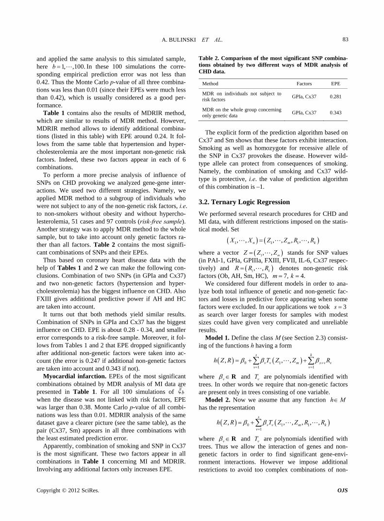
To perform a more precise analysis of influence of SNPs on CHD provoking we analyzed gene-gene inter- actions. We used two different strategies. Namely, we applied MDR m
ere not subject to any of the non-genetic risk factors, i.e. to non-smokers without obesity and without hypercho-lesterolemia, 51 cases and 97 controls (risk-free sample). Another strategy was to apply MDR method to the whole sample, but to take into account only genetic factors ra-ther than all factors. Table 2 contains the most signifi-cant combinations of SNPs and their EPEs.
Thus based on coronary heart disease data with the help of Tables 1 and 2 we can make the following con-clusions. Combination of two SNPs (in GPIa and Cx37) and two non-genetic factors (hypertension
olesterolemia) has the biggest influence on CHD. Also FXIII gives additional predictive power if AH and HC are taken into account.
It turns out that both methods yield similar results. Combination of SNPs in GPIa and Cx37 has the biggest influence on CHD. EPE is about 0.28 - 0.34, and smaller error corresponds to a risk
ws from Tables 1 and 2 that EPE dropped significantly after additional non-genetic factors were taken into ac-count (the error is 0.247 if additional non-genetic factors are taken into account and 0.343 if not).
Myocardial infarction. EPEs of the most significant combinations obtained by MDR analysis of MI data are presented in Table 1. For all 100 simulations of b when the disease was not linked with risk factors, EPE w
he
increases EPE.
Ta
E
as larger than 0.38. Monte Carlo p-value of all combi- nations was less than 0.01. MDRIR analysis of the same dataset gave a clearer picture (see the same table), as t pair (Cx37, Sm) appears in all three combinations with the least estimated prediction error.
Apparently, combination of smoking and SNP in Cx37 is the most significant. These two factors appear in all combinations in Table 1 concerning MI and MDRIR. Involving any additional factors only
ble 2. Comparison of the most significant SNP combina-tions obtained by two different ways of MDR analysis of CHD data.
Method Factors EP
MDR on individuals not subject to risk factors
GPIa, Cx37 0.281
MDR on the whole gronly gene
oup concerning tic data
G 7 PIa, Cx3 0.343
icit form of the prediction al m based
C cto nte . S ll as homozygote for of
e SNP in Cx37 provokes the disease. However wild- ty
trictions imposed on the statis-
The expl gorith onx37 and Sm shows that these famoking as we
rs exhibit irecessive allele
raction
thpe allele can protect from consequences of smoking.
Namely, the combination of smoking and Cx37 wild- type is protective, i.e. the value of prediction algorithm of this combination is –1.
3.2. Ternary Logic Regression
We performed several research procedures for CHD and MI data, with different restical model. Set
1 1 1, , , , , , ,n m kX X Z Z R R
where a vector 1, , mZ Z Z stands for SNP values (in PAI-1, GPIa, GPIIIa, FXIII, FVII, IL-6, Cx37 respec- tively) and 1, , kR R R denotes non-genetic risk factors (Ob, AH, Sm, HC), 7,m 4.k
four different
s in predictive r applications we took 3s
We considered models in order to ana- lyze both total influence of genetic and non-genetic fac- tors and losse force appearing when some factors were excluded. In ou as
nsist
, , ,Z R T Z Z R
search over larger forests for samples with modest sizes could have given very complicated and unreliable results.
Model 1. Define the class M (see Section 2.3) co - ing of the functions h having a form
s k
h 0 11 1
v v m s v vv v
where v R and vT are polynomials identified with trees. In other words we require that non-genetic factors are present only in trees consisting of one variable.
Model 2. Now we assume that any function h M represe has the ntation
0 1 1, , , , , ,s
v v m kh Z R T Z Z R R 1v
where v R and vT are polynomials identified with trees. Thus we allow the interaction of genes and non- genetic factors in order to find significant gene-envi- ronment interactions. However we impose additional
ons to torestricti avoid o complex combinations of non-
Copyright © 2012 SciRes. OJS

A. BULINSKI ET AL. 84
genetic risk factors. We do not tackle here effects of in- teractions where several non-genetic factors are involved. Namely, we consider only the trees satisfying the fol- lowing two conditions.
1) If there is a leaf containing non-genetic factor vari- able then the root of that leaf contains product operator.
2) Moreover, another branch growing from the same root is also a leaf and contains a genetic (SNP) variable.
obst e the impo
simulated annealing search of
error of 0.23 was obtained. Model 3
2 2
3 7 1 3
7
)( )
),
Z Z Z Z
with sums and products modulo 3. The non-genetic factors 2 and 4 (i.e. AH and H ) are
the most influential since the coefficients at them are the greatest ones (1.311 and 2.331). As is shown above,
. If the gene-environ- m
Models 3 and 4 have additional restrictions that poly-nomials vT 1, ,v s in (30) depend only on non- genetic factors and only on SNPs respectively. These models are considered to compare their results with ones
tained with all information taken into account, in order to demon rat rtance of genetic (resp. non-ge- netic) data for risk analysis.
Coronary heart disease. The obtained results are provided in Table 3.
EPE in Model 1 for CHD was only 0.19. For the same model we performed also fast
the optimal forest which was much more time-effi- cient, and a reasonable
application showed that non-genetic factors play an important role in CHD genesis, as classification based on non-genetic factors only gave the error less than 0.23, while usage of SNPs only (Model 4) let the error grow to 0.34.
Model 1 gave the minimal EPE. For the optimal forest 1 4, ,T R the function ,h Z R given before formula (28) with 1, ,S N is provided by
1 2 3 1
2 3 4
0.597 0.354 0.521 0.444
1.311 0.146 31 0.226
T T T R
R R R
(31)
where
2.3
1 3 4 6 7 2
2 2
2 1 3 6 7 2 4
2
3 2 2 6 7
( ( )
( ) ( ( )
2 ( )
T Z Z Z Z Z Z
T Z Z Z Z Z Z Z
T Z Z Z Z
7 ,
C
MDR yielded the same conclusionent interactions were allowed (Model 2), no consider-
able increase in predictive power has been detected. How- ever we list the pairs of SNPs and non-genetic factors present in the best forest: 7Z and 2R , 7Z and 1R ,
7Z and 4R , 5Z and 1R We see that SNP in Cx37 is of substantial importance as it appears in combination with all risk factors except for smoking.
As formula (31) is hard to i erpret, w se t nifican N via a variant of permutation test. Con-
sider a random rearrangement of the column with first SNP in CHD dataset. Calculate the EPE
nt e lect the mossig t S Ps
using these new
si
ve by MDR method.
factors play sl
mulated data and the same function h as before. The analogous procedure is done for other columns (contain- ing the values of other SNPs) and the errors found are given in Table 4 (recall that the EPE equals 0.19 if no permutation is done).
It is seen that the error increases considerably when the values of GPIa and Cx37 are permuted. The state- ment that they are the main sources of risk agrees with what was obtained abo
Myocardial infarction. For the MI dataset, under the same notation that above, the results obtained for our four models are given in Table 3. To comment them we should first note that non-genetic risk
ightly less important role compared with CHD risk: if they are used without genetic information, the error in- creases by 0.09, see Models 1 and 3 (while the same in- crease for CHD was 0.03). The function ,h Z R de- fined before (28) with 1, ,S N equals
1 2 3 1
2 3 4
1.144 0.914 0.45 0.285
0.675 0.828 0.350 0.0
T T T R
R R R
where
55
2, , T Z Z Z Z Z1 1 3 5 2 7 3 3 4 6 7T Z T Z Z .
Thus the first tree has the greatest weight (coefficient equals –1.144), the second tree (i.e. SNP in Cx37) is on the second place, and non-genetic factors are less impor-
Model 1 2 3 4
tant.
Table 3. Results of TLR.
EPE for CHD 228 0.340 0.190 0.204 0.
EPE for MI 0.305 0.331 0.391 0.365
Table 4. The SNP significance test for CHD in Model 1.
SNP permuted EPE
GPIa 0.263
Cx37 0.260
IL-6 0.226
PAI-1 0.212
G PIIIa 0.208
FXIII 0.202
FVII 0.190
Copyright © 2012 SciRes. OJS
A. BULINSKI ET AL. 85
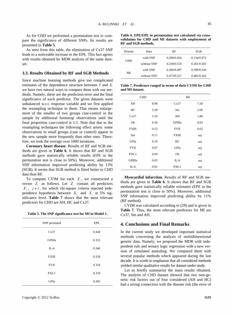
Table 6. EPE/EP ermutation test calculat cross- validation for CHD and MI datasets with em nt of RF and SGB methods.
As for CHD w ormed a permutation t com-pare the significance of different SNPs. Its res lts are presented in Tab
e machine learning methods give too complicated estimates of the dependence structure between Y and X,
-
e perf est tou
le 5. As seen from this table, the elimination of Cx37 SNP
leads to a noticeable increase in the EPE. This fact agrees with results obtained by MDR analysis of the same data-set.
3.3. Results Obtained by RF and SGB Methods
Sinc
we have two natural ways to compare them with our methods. Namely, these are the prediction error and the final significance of each predictor. The given datasets were unbalanced w.r.t. response variable and we first applied the resampling technique to them. That means enlarge-ment of the smaller of two groups case-control in the sample by additional bootstrap observations until the final proportion case:control is 1:1. Note that due to the resampling techniques the following effect arises: some observations in small groups (case or control) appear in the new sample more frequently than other ones. There-fore, we took the average over 1000 iterations.
Coronary heart disease. Results of RF and SGB me-thods are given in Table 6. It shows that RF and SGB methods gave statistically reliable results (EPE in the permutation test is close to 50%). Moreover, additional SNP information improved predicting ability by 13% (SGB). It seems that SGB method is fitted better to CHD data than RF.
To compute CVIM for each iX , we constructed a vector iZ as follows. Let iZ contain all predictors
jX , j i , for which chi-square criteria rejected inde-pendence hypothesis between jX and iX at 5% sig-nificance level. Table 7 shows that the most relevant predicto for CHD are AH, HC and Cx37.
Table 5. The SNP significance test for MI in Model 1.
SNP permuted
rs
EPE
Cx37 0.444
GPIIIa 0.353
IL-6 0.340
FXIII 0.328
FVII 0.324
PAI-1 0.319
GPIa 0.305
E in p ed viaployme
Disease Data RF SGB
with SNP 0.200/0.454 0.134/0.473 CHD
without SNP 0.230/0.510 0.261/0.503
with SNP 0.36 97 0.3 30 MI
without
0/0.4 99/0.5
SNP 0.473/0.527 0.482/0.562
Table 7. Predi ed in CV D and
CHD MI
ctors rangt.
terms of their IM for CH MI datase
AH 8.90 Cx37 7.50
HC 5.30 Sm 2.00
Cx37 5.10 AH 1.86
F
G
P
Ob 0.56 GPIIIa 0.03
XIII 0.53 FVII 0.02
Sm 0.11 FXIII 0
PIa 0.10 HC 0
FVII 0.07 GPIa 0
AI-1 0.03 Ob 0
GPIIIa 0.02 IL-6 0
IL-6 0.01 PAI-1 0
M ial infa n. Resul d SGB me-
thods ven in e 6. It s hat RF and SGB m hods gave statistically reliable estimates (EPE in the pe
we developed important statistical methods concerning the analysis of multidimensional
with inde-
of
yocard rctio ts of RF an are gi Tabl hows t
etrmutation test is close to 50%). Moreover, additional
SNP information improved predicting ability by 11% (RF method).
CVIM was calculated according to (29) and is given in Table 7. Thus, the most relevant predictors for MI are Cx37, Sm and AH.
4. Conclusions and Final Remarks
In the current study
genetic data. Namely, we proposed the MDRpendent rule and ternary logic regression with a new ver-sion of simulated annealing. We compared them with several popular methods which appeared during the last decade. It is worth to emphasize that all considered methods yielded similar qualitative results for dataset under study.
Let us briefly summarize the main results obtained. The analysis of CHD dataset showed that two non-ge- netic risk factors out of four considered (AH and HC) had a strong connection with the disease risk (the error
Copyright © 2012 SciRes. OJS
A. BULINSKI ET AL. 86
cl
tio
se requires a more detailed description of indi-vi
as well. The study can be continued anm
, R. Shimizu and V. V. Ulyanov, “Multivari-ate Statistics: High-Dimensional and Large-Sample Ap-proximations,” Wiley, Hoboken, 2010.
[2] S. Szymczak, ell, O. González- assification based on non-genetic factors only is 0.25 - 0.26 with p-value less than 0.01). Also, the classification based on SNPs only gave an error of 0.28 which is close to one obtained by means of non-genetic predictors. Moreover, the most influential SNPs were in genes Cx37 and GPIa (FXIII also entered the analysis only when AH and HC were present). EPE decreased to 0.13 when both SNP information and non-genetic risk factors were taken into account and SGB was employed. Note that exclude- ing any of the 5 remaining SNPs (all except for two most influential) from data increased the error by 0.01 - 0.02 approximately. So, while the most influential data were responsible for the situation within a large part of popu-lation, there were smaller parts where other SNPs came to effect and provided a more efficient prognosis (“small subgroups effect”). The significance of SNP in GPIa and FXIII genes was observed in our work. AH and HC in-fluence the disease risk by affecting the vascular wall, while GPIa and FXIII may improve prognosis accuracy because they introduce haemostatic aspect into analysis.
The MI dataset gave the following results. The most significant factors of MI risk were the SNP in Cx37 (more precisely, homozygous for recessive allele) and smoking with a considerable gene-environment interact-
n present. The smallest EPE of methods applied was 0.33 - 0.35 (with p-value less than 0.01). The classifica-tion based on non-genetic factors only yielded a greater error of 0.42. Thus genetic data improved the prognosis quality noticeably. While two factors were important, other SNPs considered actually did not improve the prognosis essentially, i.e. no small groups effect was ob-served.
While CHD data used in the study permitted to specify the most important predictors with EPE about 0.13, the MI data lead to less exact prognoses. Perhaps this com- plex disea
dual’s genetic characteristics and environmental fac- tors.
The conclusions given above are based on several complementary methods of modern statistical analysis. These new data mining methods allow to analyze other datasets d the
edical conclusions need to be replicated with larger datasets, in particular, involving new SNP data.
5. Acknowledgements
The work is partially supported by RFBR grant (project 10-01-00397a).
REFERENCES [1] Y. Fujikoshi
J. Biernacka, H. CordRecio, I. König, H. Zhang and Y. Sun, “Machine Learn-ing in Genome-Wide Association Studies,” Genetic Epi-demiology, Vol. 33, No. S1, 2009, pp. 51-57. doi:10.1002/gepi.20473
[3] D. Brinza, M. Schultz, G. Tesler and V. Bafna, “RAPID Detection of Gene-Gene Interaction in Genome-Wide Association Studies”, Bioinformatics, Vol. 26, No. 22, 2010, pp. 2856-2862. doi:10.1093/bioinformatics/btq529
.
[4] C. A. Stolle, I. D. Krantz, D. B. Goldstein and H. Hakonarson, “Interpretation of Associa-tion Signals and Identification of Causal Variants from Genome-Wide Association Studies,” The American Jour- nal of Human Genetics, Vol. 86, No. 5, 2010, pp. 730-742
K. Wang, S. P. Dickson,
doi:10.1016/j.ajhg.2010.04.003
[5] Y. Liang and A. Kelemen. “Statistical Advances and Challenges for Analyzing Correlated High Dimensional SNP Data in Genomic Study for Complex Diseases,” Statistics Surveys, Vol. 2, No. 1, 2008, pp. 43-60. doi:10.1214/07-SS026
[6] H. Schwender and I. Ruczinski, “Testing SNPs and Sets of SNPs for Importance in Association Studies,” Bio- statistics, Vol. 12, No. 1, 2011, pp. 18-32. doi:10.1093/biostatistics/kxq042
M. Ritchie, L. Hahn, N[7] . Roodi, R. Bailey, W. Dupont, F. Parl and J. Moore, “Multifactor-Dimensionality Red- uction Reveals High-Order Interactions among Estrogen- Metabolism Genes in Sporadic Breast Canerican Journal of Human Genetic
cer,” The Am- s, Vol. 69, No. 1, 2001,
pp. 138-147. doi:10.1086/321276
[8] D. Velez, B. White, A. Motsinger, W. Bush, M. Ritchie, S. Williams and J. Moore, “A Balanced Accuracy Fun- ction for Epistasis Modeling in Imbalanced Datasets Using Multifactor Dimensionality Reduction,” Genetic Epidemiology, Vol. 31, No. 4, 2007, pp. 306-315. doi:10.1002/gepi.20211
[9] I. Ruczinski, C. Kooperberg and M. LeBlanc, “Logic Regression,” Journal of Computational and Graphical Statiststics, Vol. 12, No. 3, 2003, pp. 475-511. doi:10.1198/1061860032238
[10] H. Schwender and K. Ickstadt, “Identification of SNP Interactions Using Logic Regression,” Biostatistics, Vol. 9, No. 1, 2008, pp. 187-198. doi:10.1093/biostatistics/kxm024
[11] L. Breiman, “Random Forests,” Machine Learning, Vol. 45, No. 1, 2001, pp. 5-32. doi:10.1023/A:1010933404324
[12] J. Friedman, “Stochastic Gradient Boosting,” Computa-tional Statistics & Data analysis, Vol. 38, No. 4, 2002, pp. 367-378. doi:10.1016/S0167-9473(01)00065-2
[13] X. Wan, C. Yang, Q. Yang, H. Xue, N. Tang and W. Yu, “Mega SNP Hunter: A Learning Approach to Detect Dis-ease Predisposition SNPs and High Level Interactions in Genome Wide Association Study,” BMC Bioinformatics, Vol. 10, 2009, p. 13. doi:10.1186/1471-2105-10-13
[14] A. Bulinski, O. Butkovsky, A. Shashkin, P. Yaskov, M. Atroshchenko and A. Khaplanov, “Statistical Methods of SNPs Analysis,” Technical Report, 2010, pp. 1-159 (in Russian).
Copyright © 2012 SciRes. OJS

A. BULINSKI ET AL.
Copyright © 2012 SciRes. OJS
87
urst
Internal Validation Techniques for Multi-
[15] G. Bradley-Smith, S. Hope, H. V. Firth and J. A. H , “Oxford Handbook of Genetics,” Oxford University Press, New York, 2010.
[16] S. Winham, A. Slater and A. Motsinger-Reif, “A Com- parison of factor Dimensionality Reduction,” BMC Bioinformatics, Vol. 11, 2010, p. 394. doi:10.1186/1471-2105-11-394
[17] A. Arlot and A. Celisse, “A Survey of Cross-Validation Procedures for Model Selection,” Statistics Surveys, Vol. 4, No. 1, 2010, pp. 40-79. doi:10.1214/09-SS054
[18] T. Hastie, R. Tibshirani and J. Friedman, “The Elements of Statistical Learning: Data Mining, Inference, and Pre- diction,” 2nd Edition, Springer, New York, 2009.
[19] R. L. Taylor and T.-C. Hu, “Strong Laws of Large Num-bers for Arrays of Rowwise Independent Random Ele-ments,” International Journal of Mathematics and Mathe- matical Sciences, Vol. 10, No. 4, 1987, pp. 805-814. doi:10.1155/S0161171287000899
[20] E. Lehmann and J. Romano, “Testing Statistical Hypo- theses,” Springer, New York, 2005.
[21] P. Golland, F. Liang, S. Mukherjee and D. Panchenko, “Permutation Tests for Classification,” Lecture NoteComputer Science, Vol. 3559, 2005
s in, pp. 501-515.
doi:10.1007/11503415_34
[22] J. Park, “Independent Rule in Classification of Multi- variate Binary Data,” Journal of Multivariate Analysis, Vol. 100, No. 10, 2009, pp. 2270-2286. doi:10.1016/j.jmva.2009.05.004
[23] S. Lee, Y. Chung, R. Elston, Y. Kim and T. Park, “Log- Linear Model-Based Multifactor Dimensionality Reduc- tion Method to Detect Gene-gene Interactions,” Bioinfor- matics, Vol. 23, No. 19, 2007, pp. 2589-2595.
doi:10.1093/bioinformatics/btm396
[24] A. Nikolaev and S. Jacobson, “Simulated AnneM. Gendreau and J.-Y. Potvin, Eds.
aling,” In: , Handbook of Meta-
aimon and L. Rokach, Eds., Data
Importance for Random
heuristics, Springer, New York, 2010, pp. 1-39.
[25] G. Biau, “Analysis of a Random Forests Model,” LSTA, LPMA, Paris, 2010.
[26] N. Chawla, “Data Mining for Imbalanced Datasets: An Overview,” In: O. MMining and Knowledge Discovery Handbook, Springer, New York, 2010, pp. 875-886.
[27] C. Strobl, A. Boulesteix, T. Kneib, T. Augustin and A. Zeileis, “Conditional Variable Forests,” BMC Bioinformatics, Vol. 9, 2008, p. 307. doi:10.1186/1471-2105-9-307
[28] A. Hirashiki, Y. Yamada, Y. Murase, Y. Suzuki, H.taoka, Y. Morimoto, T. Tajika,
Ka- T. Murohara and M. Yo-
kota, “Association of Gene Polymorphisms with Coro- nary Artery Disease in Low- or High-Risk Subjects De-fined by Conventional Risk Factors,” Journal of the Am- erican College of Cardiology, Vol. 42, No. 8, 2003, pp. 1429-1437. doi:10.1016/S0735-1097(03)01062-3
[29] A. Balatskiy, E. Andreenko and L. Samokhodskaya, “The Connexin37 Polymorphism as a New Risk Factor of MI
D. Vaughan and J. Moore,
Development,” Siberian Medical Journal, Vol. 25, No. 2, 2010, pp. 64-65 (in Russian).
[30] C. Coffey, P. Hebert, M. Ritchie, H. Krumholz, J. Ga-ziano, P. Ridker, N. Brown, “An Application of Conditional Logistic Regression and Multifactor Dimensionality Reduction for Detecting Gene- Gene Interactions on Risk of Myocardial Infarction: The Importance of Model Validation,” BMC Bioinformatics, Vol. 5, 2004, p. 49. doi:10.1186/1471-2105-5-49