Statistical methods in NLPIntroduction

Richard Johansson

January 20, 2015

-20pt

today

I course matters

I analysing numerical data with Python

I basic notions of probability

I simulating random events in Python

-20pt

overview

overview of the course

analysing numerical data in Python

basics of probability theory

randomness in Python

-20pt

why statistics in NLP and linguistics?

I in experimental evaluations:I a HMM tagger T1 is tested on a sample of 1000 words and

gets and accuracy rate of 0.92 (92%). How precise is thismeasurement?

I a Brill tagger T2 is tested on the same sample and gets anaccuracy rate of 0.94. Is the Brill tagger signicantly betterthan the HMM tagger?

-20pt

why statistics in NLP and linguistics?

I in investigations of linguistic data:I what is the probability of object fronting in Dutch?I do speakers aected by Alzheimer's disease exhibit a

signicantly smaller vocabulary?

-20pt

why statistics in NLP and linguistics?

I in language processing systems:I what is the probability of English case being translated to

Swedish kapsel?I . . . of a noun if the previous word was a verb?

I data-driven NLP systems: we specify a general model and tunespecic parameters by observing our data

-20pt

course overview

I theoretical part:I probability theoryI statistical inferenceI statistical methods in experiments

I applications in NLP:I classiers, taggers, parsers, topic modelsI machine translation (Prasanth)

-20pt

course work

I lectures in K235 or L308

I lab sessions in the new computer lab G212

I always on Tuesdays at 1012 or Thursdays at 1315

-20pt

examination

I 2 mandatory computer exercises

I 3 mandatory programming assignmentsI text categorizationI evaluationI PoS tagger implementation

I 2 optional programming assignmentsI topic modelingI machine translation

I you get a VG if you do the two optional assignments, andwrite a short essay after the second programming assignment

-20pt

deadlines

I computer exercises: a few days

I programming assignments: 2 weeks after lab session

I VG assignments: April 5

-20pt

literature

I Manning and Schütze: Foundations of Statistical NaturalLanguage Processing

I http://nlp.stanford.edu/fsnlp/

-20pt

literature linked from the web page

I Krenn and Samuelsson: The Linguist's Guide to Statistics Don't Panic!

I alternative to M&S for the theoretical part of the course

I lecture notes by Michael CollinsI for the NLP partI more in-depth than M&S

I Mitchell: Naïve Bayes and Logistic Regression

I a few other research papers

-20pt

overview

overview of the course

analysing numerical data in Python

basics of probability theory

randomness in Python

-20pt

summary statistics and plotting

I if we have some collection of data, it can be useful tosummarize the data using plots and high-level measures

I a useful skill in general when carrying out experiments

I and we'll use it in the two computer exercises

-20pt

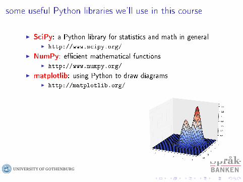
some useful Python libraries we'll use in this course

I SciPy: a Python library for statistics and math in generalI http://www.scipy.org/

I NumPy: ecient mathematical functionsI http://www.numpy.org/

I matplotlib: using Python to draw diagramsI http://matplotlib.org/

-20pt

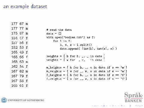
an example dataset

177 67 m

177 77 m

175 87 m

154 47 f

157 56 f

152 53 f

165 49 f

165 66 f

165 63 m

162 54 f

167 62 m

167 79 f

167 58 f

165 61 f

# read the data

data = []

with open('bodies.txt') as f:

for l in f:

h, w, s = l.split()

data.append( (int(h), int(w), s) )

heights = [ h for h, _, _ in data ]

weights = [ w for _, w, _ in data ]

m_heights = [ h for h, _, s in data if s == 'm']

m_weights = [ w for _, w, s in data if s == 'm']

f_heights = [ h for h, _, s in data if s == 'f']

f_weights = [ w for _, w, s in data if s == 'f']

-20pt

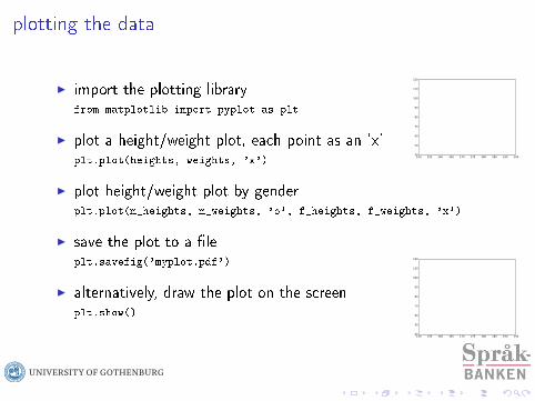
plotting the data

I import the plotting libraryfrom matplotlib import pyplot as plt

I plot a height/weight plot, each point as an 'x'plt.plot(heights, weights, 'x')

I plot height/weight plot by genderplt.plot(m_heights, m_weights, 'o', f_heights, f_weights, 'x')

I save the plot to a leplt.savefig('myplot.pdf')

I alternatively, draw the plot on the screenplt.show()

150 155 160 165 170 175 180 185 190 19540

50

60

70

80

90

100

110

120

150 155 160 165 170 175 180 185 190 19540

50

60

70

80

90

100

110

120

-20pt

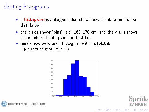
plotting histograms

I a histogram is a diagram that shows how the data points aredistributed

I the x axis shows bins, e.g. 165170 cm, and the y axis showsthe number of data points in that bin

I here's how we draw a histogram with matplotlib:plt.hist(heights, bins=10)

140 150 160 170 180 190 2000

5

10

15

20

25

30

35

40

45

-20pt

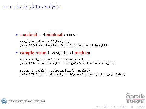
some basic data analysis

I maximal and minimal values:

max_f_height = max(f_heights)

print('Tallest female: 0 cm'.format(max_f_height))

I sample mean (average) and median:

mean_m_weight = scipy.mean(m_weights)

print('Mean male weight: 0 kgs'.format(mean_m_weight))

median_f_weight = scipy.median(f_weights)

print('Median female weight: 0 kgs'.format(median_f_weight))

-20pt

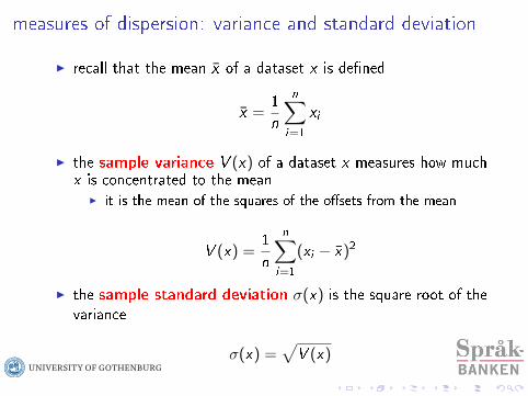
measures of dispersion: variance and standard deviation

I recall that the mean x of a dataset x is dened

x =1

n

n∑i=1

xi

I the sample variance V (x) of a dataset x measures how muchx is concentrated to the mean

I it is the mean of the squares of the osets from the mean

V (x) =1

n

n∑i=1

(xi − x)2

I the sample standard deviation σ(x) is the square root of thevariance

σ(x) =√

V (x)

-20pt

example

I low variance: data concentrated near the meanI in the extreme case: all values are identical

I high variance: data spread out

150 160 170 180 190 2000

50

100

150

200

250

300

σ = 2.9

150 160 170 180 190 2000

50

100

150

200

250

300

σ = 9.1

-20pt

variance and standard deviation in SciPy

I variance:var_height = scipy.var(heights)

I standard deviation:

std_m_weight = scipy.std(m_weights)

-20pt

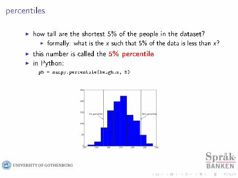
percentiles

I how tall are the shortest 5% of the people in the dataset?I formally: what is the x such that 5% of the data is less than x?

I this number is called the 5% percentileI in Python:

p5 = numpy.percentile(heights, 5)

140 150 160 170 180 190 2000

50

100

150

200

250

5% percentile 95% percentile

-20pt

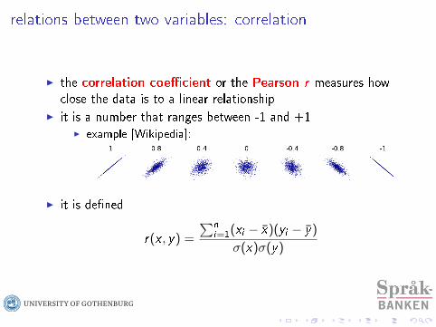
relations between two variables: correlation

I the correlation coecient or the Pearson r measures howclose the data is to a linear relationship

I it is a number that ranges between -1 and +1I example [Wikipedia]:

I it is dened

r(x , y) =

∑n

i=1(xi − x)(yi − y)

σ(x)σ(y)

-20pt

correlation example

I for the heightweight data, r = 0.87

150 155 160 165 170 175 180 185 190 19540

50

60

70

80

90

100

110

120

I with Python:correlation = scipy.stats.pearsonr(heights, weights)[0]

-20pt

overview

overview of the course

analysing numerical data in Python

basics of probability theory

randomness in Python

-20pt

what are probabilities?

I relative frequencies?I if we can repeat an experiment: how often does the event E

occur?I when we roll a die, we may say that the probability of a 4 is

1/6 because we will get a 4 approximately 1/6 of the time

I degrees of belief?I what is the probability that Elvis Presley is alive?I with which probability could Germany have won WW2?

-20pt

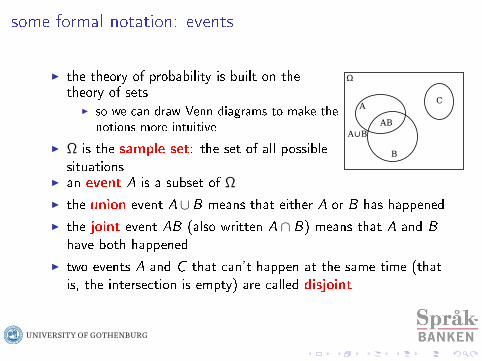
some formal notation: events

I the theory of probability is built on thetheory of sets

I so we can draw Venn diagrams to make thenotions more intuitive

I Ω is the sample set: the set of all possiblesituations

I an event A is a subset of Ω

I the union event A∪B means that either A or B has happened

I the joint event AB (also written A ∩ B) means that A and B

have both happened

I two events A and C that can't happen at the same time (thatis, the intersection is empty) are called disjoint

-20pt

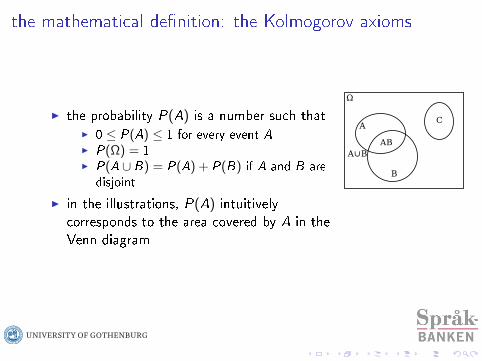
the mathematical denition: the Kolmogorov axioms

I the probability P(A) is a number such thatI 0 ≤ P(A) ≤ 1 for every event AI P(Ω) = 1I P(A ∪ B) = P(A) + P(B) if A and B are

disjoint

I in the illustrations, P(A) intuitivelycorresponds to the area covered by A in theVenn diagram

-20pt

example: Dice rolling

I A = rolling a 4; P(A) = ?

I B = rolling 3 or lower; P(B) = ?

I C = rolling an even number; P(C ) = ?

I P(A ∪ B) = P(A) + P(B)?

I P(A ∪ C ) = P(A) + P(C )?

I P(rolling 1, 2, 3, 4, 5, or 6) = ?

-20pt

some consequences

I A′ = everything but A = Ω \ A

P(A′) = 1− P(A)

P(∅) = 0

I A = rolling a 4; P(A) = ?

I A′ = not rolling 4; P(A′) = ?

I P(rolling neither 1, 2, 3, 4, 5, 6) = ?

-20pt

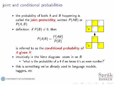
joint and conditional probabilities

I the probability of both A and B happening iscalled the joint probability, written P(AB) orP(A,B)

I denition: if P(B) 6= 0, then

P(A|B) =P(AB)

P(B)

is referred to as the conditional probability of

A given BI intuitively in the Venn diagram: zoom in on B

I what is the probability of a 4 if we know it's an even number?

I this is something we've already used in language models,taggers, etc

-20pt

example: vowels in English

I P(vowel) = 0.36

I P(vowel | previous is vowel) = 0.12

I P(vowel | previous is not vowel) = 0.50

-20pt

the multiplication rule and the chain rule

I if we rearrange the denition of the conditional probability, weget the multiplication rule

P(AB) = P(A|B) · P(B)

I if we have more than two events, this rule can be generalizedto the chain rule

P(ABC ) = P(A|BC ) · P(B|C ) · P(C )

I this decomposition is used in taggers, language models, etc

-20pt

independent events

I denition: two events A and B are independent if

P(AB) = P(A) · P(B)

I this can be rewritten in a more intuitive way: the probabilityof A does not depend on anything about B

P(A|B) = P(A)

-20pt

examples

I dice rolling:I A = rolling a 4 the rst timeI B = rolling a 4 the second time

I drawing cards:I A = drawing the ace of spades as the rst cardI B = drawing the ace of spades as the second card

-20pt

recap: the Markov assumption in language models

I unigram language model: we assume that the words occurindependently

P(w1,w2,w3) = P(w3|w2,w1) · P(w2|w1) · P(w1)= P(w3) · P(w2) · P(w1)

I bigram model: word is independent of everything but theprevious word

P(w1,w2,w3) = P(w3|w2,w1) · P(w2|w1) · P(w1)= P(w3|w2) · P(w2|w1) · P(w1)

-20pt

drawing tree diagrams (1)

-20pt

drawing tree diagrams (2)

-20pt

overview

overview of the course

analysing numerical data in Python

basics of probability theory

randomness in Python

-20pt

a brief note on random numbers

I pseudorandom numbers: generating random numbers in acomputer using a deterministic process

I usually fastI we use a starting point called the seedI if we use the same seed, we'll get the same sequence

I good for replicable experiments

I might be a security risk in some situations

I hardware random numbersI sample noise from hardware devicesI Linux: /dev/random

-20pt

basic functions for random numbers: the random library

I reset the random number generatorrandom.seed(0)

I generate a random oating-point number between 0 and 1random_float = random.random()

I generate a random integer between 1 and 6die_roll = random.randint(1, 6)

I shue the items of a list lstrandom.shuffle(lst)

I pick a random item from a list lstselection = random.choice(lst)

-20pt

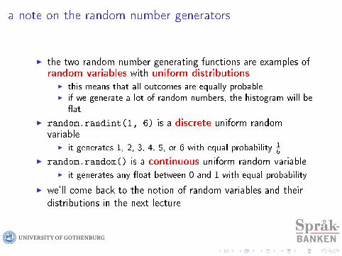
a note on the random number generators

I the two random number generating functions are examples ofrandom variables with uniform distributions

I this means that all outcomes are equally probableI if we generate a lot of random numbers, the histogram will be

at

I random.randint(1, 6) is a discrete uniform randomvariable

I it generates 1, 2, 3, 4, 5, or 6 with equal probability 1

6

I random.random() is a continuous uniform random variableI it generates any oat between 0 and 1 with equal probability

I we'll come back to the notion of random variables and theirdistributions in the next lecture

-20pt

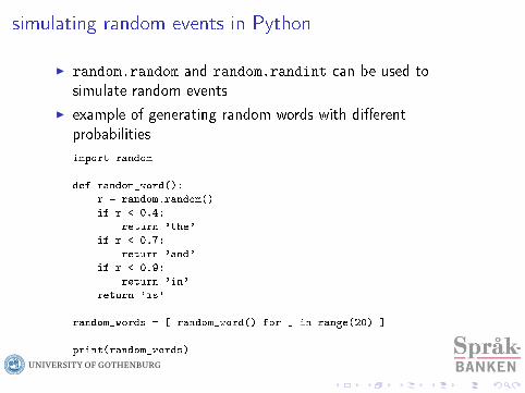
simulating random events in Python

I random.random and random.randint can be used tosimulate random events

I example of generating random words with dierentprobabilities

import random

def random_word():

r = random.random()

if r < 0.4:

return 'the'

if r < 0.7:

return 'and'

if r < 0.9:

return 'in'

return 'is'

random_words = [ random_word() for _ in range(20) ]

print(random_words)

-20pt

next lecture (Thursday)

I a few more notions from basic probability theory

I random variables and their distributions