Statistical Information Risk

Gary G. VenterGuy Carpenter Instrat

Statistical Information RiskEstimation risk

Uncertainty related to estimating parameters of distributions from data

Projection riskUncertainty arising from the possibility of future changes in the distributions

Both quantifiable to some extent

TopicsImpact of information riskEstimation risk 1 – asymptotic theoryEstimation risk 2 – Bayesian updatingEstimation risk 3 – both togetherProjection risk

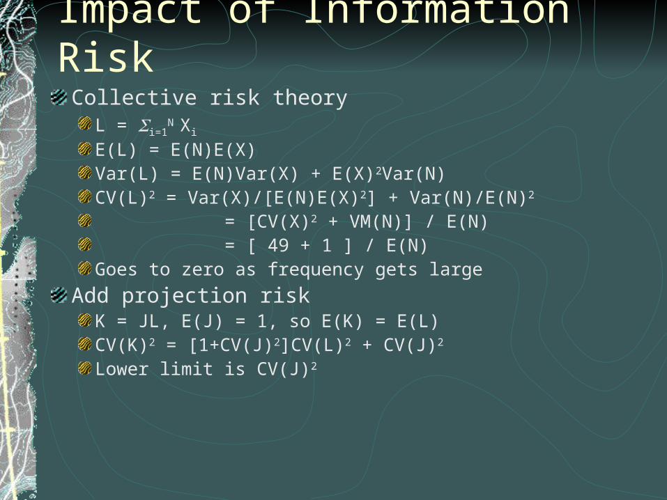
Impact of Information RiskCollective risk theory

L = i=1N Xi

E(L) = E(N)E(X)Var(L) = E(N)Var(X) + E(X)2Var(N)CV(L)2 = Var(X)/[E(N)E(X)2] + Var(N)/E(N)2 = [CV(X)2 + VM(N)] / E(N) = [ 49 + 1 ] / E(N)Goes to zero as frequency gets large

Add projection riskK = JL, E(J) = 1, so E(K) = E(L)CV(K)2 = [1+CV(J)2]CV(L)2 + CV(J)2 Lower limit is CV(J)2

Impact of Projection Risk on Aggregate CVCV(X)=7, VM(N)=1

CV(J) E(N): 2,000 20,000 200,000

0.05 16.6% 7.1% 5.2%0.03 16.1% 5.8% 3.4%0.01 15.8% 5.1% 1.9%0.00 15.8% 5.0% 1.6%

Percentiles of Lognormal Loss RatioCV(X)=7, VM(N)=1, E(LR)=65, 3 E(N)’sCV(J)=0.05 E(N)=2,000 20,000 200,000

90th 79.2 71.0 69.495th 84.1 72.8 70.899th 94.1 76.4 73.3

CV(J)=090th 78.5 69.2 66.395th 83.1 70.5 66.799th 92.5 72.9 67.4

Estimation Risk 1 – Asymptotic TheoryAt its maximum, all partial derivatives of log-likelihood function with respect to parameters are zero2nd partials are negativeMatrix of negative of expected value of 2nd partials called “information matrix”Usually evaluated by plugging maximizing values into formulas for 2nd partials Matrix inverse of this is covariance matrix of parametersDistribution of parameters is asymptotically multivariate normal with this covariance

Estimation Risk 1 – Asymptotic TheorySee Loss Models p. 63 for discussionSimulation proceeds by simulating parameters from normal, then simu-lating losses from the parametersSee Loss Models p. 613 for how to simulate multivariate normals

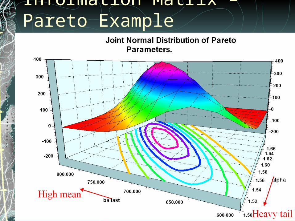
Information Matrix – Pareto Example

Estimation Risk 2 – Bayesian UpdatingBayes Theorem:

f(x|y)f(y) = f(x,y) = f(y|x)f(x)f(x|y) = f(y|x)f(x)/f(y)f(x|y) f(y|x)f(x)

Diffuse priorsf(x) 1f(x) 1/x

Estimation Risk 2 – Bayesian UpdatingFrequency Example

Poisson distribution with diffuse prior f() 1/ f(k| ) = e- k/k! f(|k) f(k| )/ e- k-1

Gamma distribution in k, 1That’s posterior; predictive distribution of next observation is mixture of Poisson by that gamma, which is negative binomialAfter n years of observation, predictive distribution is negative binomial with same mean as sample and variance = mean*(1+1/n)Parameter distribution for is gamma with mean of sample and variance = mean/nCan simulate from negative binomial or from gamma then Poisson

Estimation Risk 3 – Bayes + InformationTests developed by Rodney KrepsLikelihood function is proportional to f(data|parameters)Assume prior for parameters is proportional to 1Then likelihood function is proportional to f(parameters|data)

Likelihood Function for Small Sample Pareto Fit Scaled to Max = 1, Log Scale

Testing Assumptions of Parameter Distribution

Use information matrix to get covariance matrix of parametersThis is quadratic term of expansion of likelihood function around maxCompare bivariate normal and bivariate lognormal parameter distributions to scaled likelihood function

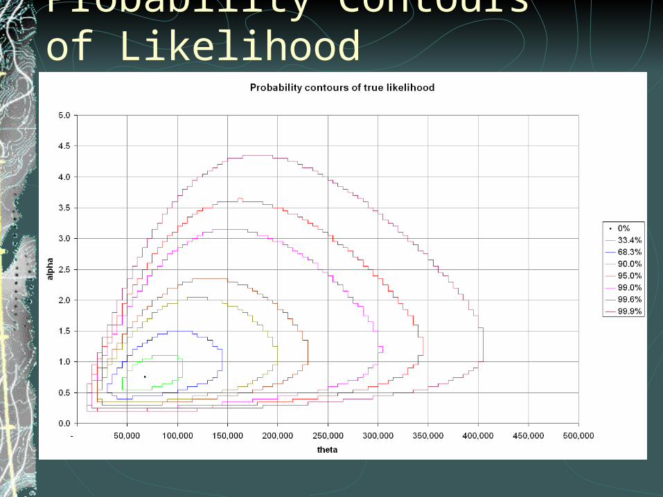
Probability Contours of Likelihood

Normal Approximation

Lognormal Approximation Contours

95th Percentile Comparison

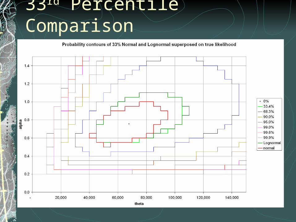
33rd Percentile Comparison

Quantifying Projection RiskRegression 100q% confidence intervals

t(q/2;N-2) is the upper 100(q/2)% point from a Student “T” distribution with N-2 degrees of freedom

Nxx

xx

NtxxYfor

Nxx

xx

NtxxYEfor

Nxxtfor

ii

Nq

ii

Nq

ii

Nq

22

2

2;2/

22

2

2;2/

222;2/

11ˆˆˆ:|

1ˆˆˆ:|

ˆˆ:

xY2

ˆ 2

N

SSE

Projection Risk Example

finis