Department of Information Technology

Statistical Football Modeling

A Study of Football Betting and Implementationof Statistical Algorithms in Premier League

Jonas Mirza, Niklas FejesSupervisor: David Sumpter

Project in Computational Science: Report

January 29, 2016

PROJECTREPORT

Contents

1 Introduction 21.1 Making money on football betting? . . . . . . . . . . . . . . . . . . . . . . 21.2 Betting and bookmaking . . . . . . . . . . . . . . . . . . . . . . . . . . . . 21.3 Problem description . . . . . . . . . . . . . . . . . . . . . . . . . . . . . . 3

2 Theory 32.1 Odds and probabilities . . . . . . . . . . . . . . . . . . . . . . . . . . . . . 32.2 Poisson and Skellam distributions in football . . . . . . . . . . . . . . . . 52.3 The Kelly Criterion . . . . . . . . . . . . . . . . . . . . . . . . . . . . . . 7

Three outcome bets . . . . . . . . . . . . . . . . . . . . . . . . . . . . . . 82.4 Multinomial Logistic Regression . . . . . . . . . . . . . . . . . . . . . . . . 9

3 Methods 113.1 Expected Goals . . . . . . . . . . . . . . . . . . . . . . . . . . . . . . . . . 11

Idea . . . . . . . . . . . . . . . . . . . . . . . . . . . . . . . . . . . . . . . 11Implementation . . . . . . . . . . . . . . . . . . . . . . . . . . . . . . . . . 12

3.2 Elo model . . . . . . . . . . . . . . . . . . . . . . . . . . . . . . . . . . . . 13Idea . . . . . . . . . . . . . . . . . . . . . . . . . . . . . . . . . . . . . . . 13Implementation . . . . . . . . . . . . . . . . . . . . . . . . . . . . . . . . . 14

3.3 Odds Bias . . . . . . . . . . . . . . . . . . . . . . . . . . . . . . . . . . . . 14Idea . . . . . . . . . . . . . . . . . . . . . . . . . . . . . . . . . . . . . . . 14Implementation . . . . . . . . . . . . . . . . . . . . . . . . . . . . . . . . . 15

3.4 Random betting model . . . . . . . . . . . . . . . . . . . . . . . . . . . . . 163.5 Data and data sources . . . . . . . . . . . . . . . . . . . . . . . . . . . . . 16

4 Results 174.1 Model comparison . . . . . . . . . . . . . . . . . . . . . . . . . . . . . . . 174.2 Odds Bias . . . . . . . . . . . . . . . . . . . . . . . . . . . . . . . . . . . . 184.3 Web application . . . . . . . . . . . . . . . . . . . . . . . . . . . . . . . . 19

5 Conclusions 19

6 Discussion 196.1 Problems . . . . . . . . . . . . . . . . . . . . . . . . . . . . . . . . . . . . 19

Selection of bookmakers . . . . . . . . . . . . . . . . . . . . . . . . . . . . 19Validation . . . . . . . . . . . . . . . . . . . . . . . . . . . . . . . . . . . . 20Odds Bias . . . . . . . . . . . . . . . . . . . . . . . . . . . . . . . . . . . . 20

6.2 Improvements . . . . . . . . . . . . . . . . . . . . . . . . . . . . . . . . . . 20

1

1 Introduction

1.1 Making money on football betting?

This report covers our work on football betting and starts with a brief introduction tothe field followed by some needed theory. Thereafter, the implementation of the threedifferent models we have been studying will be covered, to finish with our results anddiscussion.

The idea for all the models is taken from the book Soccermatics1 written by our super-visor David Sumpter.

The main goal in our work was to test and improve different betting methods andexamine the possibility to make money in the long run. This was done by buildingmathematical models, based on statistics, which exactly tell how to place the money.All our models performed better than a random-betting model and one of the modelswas able to make money during the validation period.

1.2 Betting and bookmaking

There are plenty of different scenarios that one can bet on when it comes to sports.For any given Premier League game one can easily find over 100 different types of bets,everything from who will win to who will receive the first yellow card. However, in thisproject, only bets of the type “singles” in Premier League were analyzed. A single betis a bet placed on just one selection. In football that yields win, draw or loss (1, X, 2),from a home team point of view.

A typical single bet can look something like (1.72, 3.80, 4.50) which means one have achance to win 1.72 times the money if betting on home win and so on. So how do thebookmakers set the odds? If gambling had been a fair game the odds should correspondto the estimated probability for the outcome they represent. In this case home winwill give 1.72 the money and therefore the probability for it would be its inverse 0.58.However, this is not the case and a simple example can show why. If one takes theinverse and sums up the probabilities for all the outcomes in one game one expects thesum to be equal to one, but for the bets stated above the sum is 1.07 which means thereis a 7% margin added by the bookmakers. Further on, the bookmakers have no realinterest in predicting the outcome themselves. On Wikipedia one can read:

“A bookmaker strives to accept bets on the outcome of an event in the right pro-portions so that he makes a profit regardless of which outcome prevails.”

2

1ISBN: 97814729241242https://en.wikipedia.org/wiki/Mathematics_of_bookmaking (25/1 2016)

2

This implies that the odds will be adjusted accordingly to the demand and that the givenodds rather represent the public opinion about the outcome than the “true probability”.In conclusion, if one could formulate a method that predicts the outcomes better thepublic opinion plus the bookmaker’s margin one could make money from betting.

1.3 Problem description

The idea of this project is to analyze three different betting models and examine if itis possible to use them to make money in the long run. A big part of the project wasalso to create a live web application that presents our results and shows how the modelsperform in the current and future seasons of Premier League.

A necessary condition to make money in the long run is that the model’s predictionp∗ must give a better prediction of the outcome compared to the odds b. To havea chance to succeed with this task the models need to have a statistical foundation.Therefore, the analyzed problem can be formulated as follows: Create a model that useshistorical football data and returns a set of prediction values, for (1, X, 2), that predictsthe outcome better than b.

2 Theory

2.1 Odds and probabilities

The odds we are using are given in a format known as “European style” in the gamblingcommunity, which for a fair (no-margin) bet is given as odds = 1/P(win) as described inthe introduction. While it is impossible to know exactly how the bookmakers set theirodds, we should not assume that they are setting the odds by the best possible predictionof the match outcomes. Instead, they most likely weight together their own predictions;how much money they receive in bets for each outcome; and how other bookmakers haveset their odds.

What we can do however, without confining ourselves, is to pretend that the oddsrepresent those given by a naive bookmaker who has predicted the match outcomes toher best, set the odds as the reciprocal of the probability, and scaled them down bysome percentage to take a revenue only on the winning bets. Formulating this modelmathematically gives the motivation for computing the probabilities as P(home)

P(draw)P(away)

=

1/odds1

1/oddsX1/odds2

· 1∑i∈{1,X,2} 1/oddsi

,

3

where the normalizing factor is needed in order to remove the margin from the odds. Ifthe match results were to be distributed exactly by these probabilities, we would alwayslose in the long run due to the bookmaker’s margin. This is easily seen in the followingexample:

Let p be the probability of outcome A in a game with two outcomes (A or B).The odds bA is, as previously described, set by the bookmaker as

bA = 1/p · (1−m) (1)

where m is the bookmaker’s margin such that 0 < m < 1. The expected net gainwhen betting x units is then

E[“net gain”] = p · ((bA − 1)x)− (1− p) · (−x) = (pbA − 1)x.

Inserting Equation 1 then gives us

E[“net gain”] = −mx.In the example the same equation applies for the odds on outcome B, and in general toall odds on a game with any number of outcomes. This implies that however we placeour bets the average net gain will tend towards −mx where x is the total amount webet, and we are expected to lose in the long run.

However, our assumption was that the bookmakers do not set their odds by the bestpossible predictions, so we should not assume that Equation 1 holds. If we can improvethe estimates in any way we can make a net gain on the odds.

We can study these odds probabilities by looking at the historical odds that the book-makers have set in the last years. Figure 1 shows the probabilities derived from the bestavailable odds for the 2648 games played in Premier League between 2004 and 2015.

P(home)0 0.5 1

P(away)

0

0.5

1

P(home)−P(away)-1 -0.5 0 0.5 1

P(draw)

0

0.25

0.5

0.75

Figure 1: Scatter plot of the probabilities of home win versus away win in 2648 Premier Leaguegames.

4

It is clear that the bookmakers prefer to put their probabilities close to a fixed curvein the “home-away” plane, since the probability coordinates in theory could be placedanywhere in the triangle under the dotted diagonal line between (0, 1) and (1, 0) in theleft plot.

In the left plot, the probability of draw P(draw) for a coordinate (P(home),P(away)) canbe seen as the shortest distance between the diagonal line where P(home)+P(away) = 0.This can be derived from the sum of the three possible outcomes, i.e.

P(home) + P(draw) + P(away) = 1.

The right plot in Figure 1 shows the probability for draw versus the difference betweenthe probabilities for win for either team. The transform between the two projections islinear, such that the shape of the curve is the same in both plots. The projection inthe right plot [P(home) − P(away) vs. P(draw)] is useful for visualizing how an odds-based model transform the probabilities, since the variable on the x-axis can be seen asa measure of the home team advantage on a scale from −1 to 1. Another projectionone can use is to plot P(home win | ¬draw) on the x-axis which yields a visually similarplot. In the rest of the report we have chosen to use the difference projection since it isslightly easier to use.

2.2 Poisson and Skellam distributions in football

A common way to model a football game is to assume that the expected number of goalsa team will make is given by a Poisson distribution. This assumption aligns well withthe actual match results, which can be seen from the histograms in Figure 2.

0 1 2 3 4 5 6 7 8 9

Home goals

0

500

1000

1500

2000

Number

ofgames

HistoricalPois(µH = 1.53)

0 1 2 3 4 5 6 7 8 9

Away goals

0

500

1000

1500

2000 HistoricalPois(µA = 1.12)

-6 -4 -2 0 2 4 6 8

Home goals − Away goals

0

500

1000

1500Historical

Skellam(µH ,µA)

Figure 2: Plots showing that the distribution of the number of goals in the matches in 2003–2014resembles a Poisson distribution.

The distribution of goals for the home team appears to have the same pattern, and byfurther assuming that the number of goals for the home team (X) and away team (Y )

5

are Poisson distributed, i.e.

X ∼ Pois(µ1) and Y ∼ Pois(µ2),

we get that the probability for home win and draw are

P(home) = P(X − Y > 0) and P(draw) = P(X − Y = 0).

The distribution of the difference between two independent random variables with Pois-son distribution is known as the Skellam distribution, i.e.

X ∼ Pois(µ1), Y ∼ Pois(µ2) =⇒ (X − Y ) ∼ Skellam(µ1, µ2).

This distribution can be used in a very simple model for a game, where the number ofgoals for each team are modeled as independent variables with Poisson distribution, ofexpected value µ1 and µ2. Since (X + Y ) ∼ Pois(µ1 + µ2), we can further constrain themodel by assuming that the expected value of the total number of goals µ = µ1 + µ2 isconstant. In Figure 3 the contour lines where µ are constant are shown.

P(home)−P(away)-1 -0.8 -0.6 -0.4 -0.2 0 0.2 0.4 0.6 0.8 1

P(draw)

0

0.1

0.2

0.3

0.4

0.5

µ1 + µ2 = 1.00

µ1 + µ2 = 2.00

µ1 + µ2 = 2.59

µ1 + µ2 = 3.00

µ1 + µ2 = 4.00

data

Figure 3: Blue lines have constant expected number of goals (µ1+µ2 = K). At the dotted diag-onal lines, the probability that one of the teams will make no goal is 1, and thus the probabilityof the other team winning is their probability of making at least one goal.

In Figure 3 we can see that the bookmakers set their odds approximately as the pre-dictions of this model. The contour line for µ = 2.59 is shown in the plot, which is theaverage number of goals per match over the last 10 years. The probability for draw isplaced somewhat higher than a “pure” Poisson distributed match would suggest, whichmight depend on many other factors. For example a team with a low number of expectedgoals may play defensive against a better team and aim for a draw rather than a win.In Figure 2 the histograms suggest that the probability of one team making no goals isslightly higher than predicted by the Poisson distribution, which could be a reason toslightly raise the probability of draw.

6

2.3 The Kelly Criterion

There is a well-known formula in the betting community known as the Kelly Criterion,which is an equation for computing the optimal bet to place in order to maximize theexpected outcome, given odds and outcome probabilities as input.

The Kelly Criterion is stated as follows when we have a two-outcome game where theresults are A or B, and the variables are:

pA, pB – probabilities of either outcome, such that pA + pB = 1,

BA, BB – odds (European style format),

xA, xB – fraction of payroll to bet on A or B, given that you decide to bet on one (andonly one) outcome.

The formula states that in order to maximize the long-term expected gain, the optimalfraction to bet is given as

xA =pABA − 1

BA − 1and xB =

pB BB − 1

BB − 1.

If xA ≤ 0 you should not bet on A, since you are not allowed to place a negative betwith the same odds.

The formula is easily derived by finding xA that maximizes the expected value of thelogarithm of the “net wealth when playing on A”, WA. This value is the multiplicativechange in size of the payroll, and for a game played on outcome A it is defined as

WA =

{1− xA +BA xA if win,1− xA otherwise.

The Kelly Criterion then gives the solution to the maximization problem

argmaxxA

E[log(WA)] = argmaxxA

pA log(1− xA +BA xA) + pB log(1− xA). (2)

The reason for optimizing this expected value can be derived from expected utilitytheory3 which uses the idea that the value of the gain should not be proportional tothe monetary value, but rather the utility of the money. In short, one should in eachgame try to maximize the utility (in this case the logarithm) of one’s wealth instead ofthe wealth itself. For example if your wealth is $100; losing $99 is far worse for yourlong-time betting compared to the gain you get by winning the same amount. In thiscase a 51% chance of winning would make the expected value of WA (without the utility)larger than 1, so the statistics tells you to bet as much as you can. If one instead usesthe expected value of the utility, the equations will balance out the risks over the gainsin a way that is more sensible in the long run.

3http://plato.stanford.edu/entries/rationality-normative-utility/

7

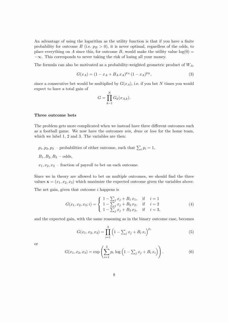
An advantage of using the logarithm as the utility function is that if you have a finiteprobability for outcome B (i.e. pB > 0), it is never optimal, regardless of the odds, toplace everything on A since this, for outcome B, would make the utility value log(0) =−∞. This corresponds to never taking the risk of losing all your money.

The formula can also be motivated as a probability-weighted geometric product of WA,

G(xA) = (1− xA +BA xA)pA (1− xA)pB , (3)

since a consecutive bet would be multiplied by G(xA), i.e. if you bet N times you wouldexpect to have a total gain of

G =

N∏k=1

Gk(xA,k).

Three outcome bets

The problem gets more complicated when we instead have three different outcomes suchas a football game. We now have the outcomes win, draw or loss for the home team,which we label 1, 2 and 3. The variables are then:

p1, p2, p3 – probabilities of either outcome, such that∑

i pi = 1,

B1, B2, B3 – odds,

x1, x2, x3 – fraction of payroll to bet on each outcome.

Since we in theory are allowed to bet on multiple outcomes, we should find the threevalues x = (x1, x2, x3) which maximize the expected outcome given the variables above.

The net gain, given that outcome i happens is

G(x1, x2, x3; i) =

1−

∑j xj +B1 x1, if i = 1

1−∑

j xj +B2 x2, if i = 2

1−∑

j xj +B3 x3, if i = 3,

(4)

and the expected gain, with the same reasoning as in the binary outcome case, becomes

G(x1, x2, x3) =

3∏i=1

(1−

∑j xj +Bi xi

)pi(5)

or

G(x1, x2, x3) = exp

(3∑

i=1

pi log(

1−∑

j xj +Bi xi

)). (6)

8

If we limit ourselves to only one bet (x1, x2, or x3), which should be positive, we findthat the optimal bet is given by the same equations as in the binary case

xi =piBi − 1

Bi − 1. (7)

If multiple xi’s are positive, we should choose the one which has the highest gainG(x1, x2, x3). It should be noted that G(x1, 0, 0) > G(0, x2, 0) does not imply thatx1 > x2; and if we have two positive xi’s the optimal combined bet is not given by theformula above.

We thus have a formula for computing the optimal fraction of one’s bankroll to placeon a 1X2-bet given that we have an estimate of the true probabilities of each outcomeand the odds received on the wager. The odds Bi are given by the bookmakers, so whatremains is to find good approximations of pi. In the rest of the report we drop the index,and denote the set of these three probabilities as p∗.

The Kelly Criterion is useful for evaluating the long-term performance of a bettingmodel, and in the project we have been using it in order to evaluate the models we haveimplemented.

2.4 Multinomial Logistic Regression

In order to use the odds to predict the actual outcomes, which we do in the Odds Biasmodel (Section 3.3), we need to use some method to fit the odds to the results. Thisproblem is non-trivial in several ways, specifically that we have three discrete outcomesin a game, that the odds themselves are not good linear predictors, and that we need tospecify a model that cannot be too general since the number of games in the last seasonsare few from a computational perspective.

We have investigated a couple of different algorithms, and the most prominent has beenmultinomial logistic regression (MNR) implemented by MATLAB’s mnrfit. The alter-natives to this method are the generalized linear models present in MATLAB (glmfit,stepwiseglm, etc.) but since these only take binary outcomes we decided to use MNRinstead of weighting together three binary models. MNR is similar to binomial logisticregression, which is the standard way to fit a predictor to a binary outcome, but insteaduses a multinomial distribution.

In order to make a fit we need a model. In short, it should take the odds for homewin, draw and away win, and output the three probabilities for each outcome. While wecould simply feed the odds directly into the MNR, this would not be able to make goodpredictions since we do not expect the odds to be linearly dependent on the probabilityof the outcomes. We therefore should preprocess the odds in some way to get a modelthat is valid through dimensional analysis. Figure 4 shows the basic flowchart for themodel.

9

odds predictors MNR probabilities

Figure 4: Flowchart for the model.

To convert the odds to predictors we take the following steps:

1. odds: The odds are taken directly from the source, see Section 3.5.

2. odds probability: The odds are converted to probabilities, by the formula assumingthat the bookmakers odds are based on a fair game. (See Section 2.1.)

3. predicting probabilities: In this step we choose which odds probabilities to usefor the prediction. In addition to the three outcome probabilities, we found thatadding P(favorite win) as a predicting variable improves the results significantly.

4. logit predictors: In the final step before the MNR we transform the probabilitiesby the logit function, defined as logit(p) = log(p/(1− p)). (See motivation below.)

In a (binomial) logistic regression, we are essentially doing a linear fit of a predictorto the logit of the outcome probabilities. Since the predictors are also probabilities,it is reasonable to apply the logit function to them before we use them, giving us thefollowing model in the binary case.

logit(p∗) = β0 + β1logit(p).

This model has the benefit that the probabilities are always in the range (0, 1), and itthus weights the variable in a more sensible way than just using the probabilities. Forexample, input probabilities of 0 or 1 will map to ±∞ (in the linear model space), andthe model will never be able to output unreasonable values such as −0.1 or 1.1. In themultinomial case the softmax function is used instead of the logistic function, and theequations are changed accordingly.

The motivation for using P(favorite win) as predicting variable comes from that we, byinspection, think that the peak in the draw probability curve (Figure 6 (a)) is lower thanit should be and that it not necessarily must be smooth for even matches. The favoritewin probability, defined as

P(favorite win) = max(P(home win),P(away win))

introduces the non-linearity seen in Figure 6 (b), and allows the MNR fit to model anon-smooth peak.

In short, the full model is then described by the following equations. Let the vectorcontaining the predictors (x1, x2, x3, . . . ) be

X =[

1 x1 x2 x3 · · ·]T,

10

and the training parameters be

β =

[β1

0 β11 β1

2 β13 · · ·

β20 β2

1 β22 β2

3 · · ·

].

Then the probabilities p are computed as

p =

exp(η1)exp(η2)

1

· 1

exp(η1) + exp(η2) + 1, where η =

[η1

η2

]= β X.

It should be noted that this equation is essentially the softmax function4.

MNR will attempt to find the parameters β such that the model predicts the trainingdata as good as possible, which is all done in Matlab’s mnrfit. There are further severaltraining parameters that can be tuned, which are discussed in MATLAB’s manual.

3 Methods

This section covers the implementation of the three models that has been studied in thisreport, namely the Expected Goals model, the Elo model, and the Odds Bias model. ACommon feature for all the three models is that they return a set of p∗. By the help ofthe Kelly criterion the models can then be evaluated and the fraction of one’s payroll tobet can be established.

3.1 Expected Goals

Idea

A rather popular model type in the football world is the Expected Goals model. Themodel attempts to predict how many goals each team will make during their encounterand estimate p∗ based on that. The model uses “shots on goal” as input data and returnsthe expected number of goals for a team. And by the use of the Skellam distribution p∗

will be obtained.

4https://en.wikipedia.org/wiki/Softmax_function

11

The reason why this model type gained ground is that models that uses “goals” as inputdata needs a very large data set in order to have a low variance. A large data set impliesthat the model takes matches from a wide time span and will therefore not be trendsecretive. If one instead uses “shots on goal” an equal large data set can be obtained injust a few matches since there are far more shots on goals compared to goals. Modelsthat are based upon expected goals can therefore be expected to be more trend sensitivecompared to goal models. In this case trend sensitivity refers to how long time it takesfor a model to adjust when a dramatic change happens in the league. A typical dramaticchange can be; a key player quits, a new coach etc.

A crucial part of this model is to be able to transform “shots on goals” into “goals” andthis was done in the following fashion. Old data that showed from where a shot hadbeen kicked and whether it was a goal or not were gathered. A specific function wasthen fitted to the data in such way that the function had the shot positions as input andreturned the probability of making a score from that very position (pg).

If one now is interested in predicting a specific encounter one simply takes the shotdata for a few matches back in time for both of the team, plug every shot into the fittedfunction and sum up the probabilities, and one ends up with the expected number of goalsfor both the teams. This numbers can then be plugged in to the Skellam distributionwhich will return p∗.

Implementation

All shot data for Premier League were loaded into MATLAB. The football pitch wasthen divided into an 40× 40 equal sized rectangular grid. A 3D histogram that showedthe relative goal frequency for every rectangle was created, see Figure 5.

It was noticed that the graph in Figure 5 reminded of a function that describes the goalangle (θ) from a certain location (xk). Let u and v denote the vectors from xk to the goalposts. Then the goal angle can be defined as θ = u·v

|u||v| . A constant c was then optimizedin such way that c · θ gave the best fit to the 3D histogram. pg was then computed aspg = c · θ.

Shots from the validation year were then loaded in MATLAB and a few games back intime were used as input to pg and summed up to determine the Expected Goal for bothteams in a given encounter. This number was fed into the Skellam distribution and p∗

was obtained.

12

Figure 5: 3D histogram of the probability to score from a given box.

3.2 Elo model

Idea

A common rating system in all types of sport is named after its creator Arpad Elo5.The system was first developed to rate chess players but has evolved through the yearsand is now used to rate everything from football to e-sports.

The idea is that every player/team has an Elo-rating, a number, corresponding to theirskill level. If a team with a high score plays against a team with a lower scorer, the betterteam i.e. the team with a higher score, is expected to win and will thus not increase theirrating by much if they win. The team with the lower score however will not be expectedto win and will be awarded a lot of points in the event they do. In this fashion theElo-table will get updated. The Elo-table can then be used to predict the outcome of agiven encounter.

Since the Elo-model was developed for chess, which is a game with binary outcomes, wemade some tweaks in order to apply it on Football. This was done by first applying thebinary Elo-model to the encounter and then use old data to estimate the probability fordraw. Finally half the probability for draw was subtracted from both the probability ofwin and lose so that the whole set sums to one.

5https://en.wikipedia.org/wiki/Elo_rating_system

13

Implementation

All match data for Premier League were loaded into MATLAB where all the teams inthe league were designated the same Elo-score. The Elo-table was then updated by theuse of all the match result data in the time interval, in the following way. Let T1 andT2 denote the teams old Elo-rating and Tn1 and Tn2 denote their new Elo-rating after agiven encounter.

If then T1 wins the encounter, their new Elo will be

Tn1 = T1 + 40

(1− 1

1 + 10T2−T1400

)and Tn2 will be

Tn2 = T1 + T2 − Tn1,

and vice versa if T2 wins.

If the match was a draw

Tn1 = T1 + 40

(1

2− 1

1 + 10T2−T1400

)and vice versa for T2.

With the updated Elo-table the probability for win, loss (W,L), for T1, can be calculatedas:

W = 1− 1

1 + 10T2−T1400

since this is the very same distribution used to score the teams with in the first place,and then L = 1−W , this given a zero probability for draw.

To get the probabilities for win, draw, and loss (p∗1, p∗X , p

∗2) one have to adjust for the

draw probability. This was done by fitting historical outcomes to historical odds by theuse of MNR. The odds were then interpreted as probabilities and P(draw) was plottedagainst P(home win | ¬draw). This plot was then used to get p∗X as a function of W

and L. p∗1 and p∗2 was then given by subtractingp∗X2 from W and L.

3.3 Odds Bias

Idea

In the other two models we have used rankings and expected goals in order to get p∗ butwhat if we use the odds to approximate p? We can easily get a set of probabilities fromthe odds as described in Section 2.1, but directly applying the Kelly Criterion to thesewill, due to the bookmaker’s margin, result in that no bet is expected to be profitable.

14

Section 2.1 also shows the distribution of these probabilities, and if we add the actualmatch outcomes after binning them, we get the plot shown in Figure 6 (a). To implementthe binning, we sort the odds by P(home)−P(away), divide them into equally sized bins,and compute the average number of draw games in each bin. This will give a good visualrepresentation of the match outcomes, and it should approximate the discrete outcomesused in the MNR.

The idea behind the Odds Bias model is that in the last few years, the trend line in theodds has not been well-aligned with the actual outcome of the matches. In Figure 6 thiscan be seen from that many of the bins for even games, where P(home)− P(away) ≈ 0,are above the odds trend line.

-1 -0.5 0 0.5 1

P(home win) − P(away win)

0.1

0.2

0.3

0.4

0.5

P(draw)

Odds probabilites

Trend line

Binned outcomes

-1 -0.5 0 0.5 1

P(home win) − P(away win)

0.1

0.2

0.3

0.4

0.5

P(draw)

Corrected probabilities

Corrected trend line

Binned outcomes

(a) Trend and odds. (b) Model fit.

Figure 6: Visualization of the odds. The odds used are the maximum of the four biggestbookmakers from 2011–2014, and each bin represents the average 30 games.

Implementation

The theory and mathematical model is described in Section 2.4. In short, we perform aregression (MNR) based on the historical odds for a few years back. We decided to usethe seasons 2011–2014, since this gives us 1520 matches to train our model on. Usingmore seasons would make the fit less sensitive to noise, but on the contrary it would notbe able to catch the trends that have appeared in the last few years.

Figure 6 (b) shows how the trend line and the probabilities are moved after the fit. Thenon-smooth peak in the middle of the fit is due to a non-linearity we introduced in orderto remove the assumption that the curve should be smooth when P(home)−P(away) = 0,see Section 2.4 for details. While this may seem to contradict the Skellam distributionbased model we discussed in Section 2.2, we are in this model trying to make a fit to theactual data, and not the theoretical model.

15

The model was trained with MATLAB’s mnrfit implementation, and the fit has shownpromising results when used in the 2015/2016 season.

3.4 Random betting model

In order to analyze the models in the Sections 3.1 to 3.3 a random betting model wasdeveloped. The model was created in order to have an information free model whichimplies that anything that performed better than this model contained some sort ofinformation.

The random betting model randomly picked a a set of p∗ from a distribution createdfrom the odds curve, the curve in Figure 1.

3.5 Data and data sources

In order to collect data about the matches we have been using several different sources.The sources we have been using for the historical odds are from football-data.co.uk6

which provides weekly updated csv files with historical odds given by many differentbookmakers, as well as maximum and average odds.

This data also contains information such as number of shots on goal, number of corners,half-time and full-time scores, number of fouls, and number of red and yellow cards.

There are some problems with this data though, and that is that different bookmakershave different ways of earning money. Just looking at the highest odds available at any ofthe over 20 sites that one can play at might be misleading, since some bookmakers requirethat you to pay a certain percentage when you deposit your money, and some mightrequest you to place a certain amount to be able to get the best odds. Therefore, for ourtraining, we have only been using the maximum odds by the four biggest bookmakers.This should ideally reduce the noise in the data, caused by odds adjusted for localmarketing offers.

We have been using clubelo.com7 to get historical Elo-ratings in addition to the ones wehave computed ourselves from the match results. This site provides an API for retrievingElo-ratings for all Premier League teams and games, as well as for most other leagues.While there are other team rankings to be found on the web, this one was the easiest touse and the difference between Elo-rankings from different sources should be small sincethe equations are the same.

6http://football-data.co.uk/englandm.php7http://clubelo.com

16

4 Results

This section starts with evaluations for all the models during the same time span, thisin order to be able to compare them. Next, we continue with further evaluations of theOdds Bias model to end with a short presentation of the web application that was built.All plots in this section shows the gain, in percent, as a function of number of games.This implies that if a validation is above the zero-line it has gained money, and if it isbelow it is losing money. Due to the nature of the Kelly criterion we will never be ableto lose more than 100%, which is why some of the plots are presented with the y-axis inlog scale.

4.1 Model comparison

The models were set up with a calibration interval from 2007–2010 and then validatedfrom 2011–2014. The odds that were used were the best odds from footballdata.co.uk.Figure 7 shows these validations, by the use of the Kelly criterion, in semi-logarithmicplots.

0 100 200 300

game number

10 -40

10 -20

10 0

10 20

log(gain)

2011

Odds bias

Elo rating

Expected goals

Random

0 100 200 300 380

game number

10 -40

10 -20

10 0

10 20

log(gain)

2012

0 100 200 300 380

game number

10 -40

10 -20

10 0

10 20

log(gain)

2013

0 100 200 300 380

game number

10 -40

10 -20

10 0

10 20

log(gain)

2014

Figure 7: Four semi-logarithmic evaluations, by the use of the Kelly criterion, of how well themodels would have performed from 2011–2014.

17

In Figure 7 it can be noticed that the Elo- and Expected Goals- models evaluation, aftera few steps, lies between the zero line and the evaluation of the random model. Furtheron the validation of the Odds Bias model lies on or above the zero line.

4.2 Odds Bias

Since the Odds Bias model evaluation is over the zero line in figure 7 the same evaluations,for 2012–2015, is presented in Figure 8 but now with linear axis.

0 100 200 300 380

game number

0%

200%

400%

600%

gain

2012

2013

2014

2015

Figure 8: Linear evaluation, by the use of the Kelly criterion, of the Odds Bias models perfor-mance from 2012 to 2015.

Note that the evaluations is above the zero line for all years except of 2013.

As expected the evaluation differed when the predictors in the regression were changed.Figure 9 shows the evaluation of two Odds Bias models with different predictors. Itshould be noted that the choice of predictors is not trivial since too many predictorswill lead to overfitting, and using linearly dependent predictors will make the MNR fitmisbehave. The calibration interval was 2011–2014 and they were validated for 2015.

0 50 100 150 200

game number

0%

100%

200%

300%

400%

gain

Premier League 2015

Model 1

Model 2

Figure 9: Linear evaluation, by the use of the Kelly criterion, of the Odds Bias models perfor-mance during 2015. The blue line corresponds to using (win, draw, lose) as predictors, and thered line corresponds to (win, draw, lose, favorite).

18

As can be seen in Figure 9 the two evaluations differ. The blue line is smoother thanthe red one but do not rise as high. The smoothness in Model 1 can be explained bythe fact that the predicted probabilities are closer to the odds probabilities, so the betswill in general be smaller. The increased profit in Model 2 comes mostly from the evenmatches, which indicates that those games are modeled better than in Model 1.

4.3 Web application

The web application that was built as a part of this project can be found at: www.

betamatics.com. It contains an evaluation of the Odds Bias model that updates everyday, as well as a table over which bets to place for the next week. There is also a“Strategies” section that briefly explains how the Odds Bias- as well as the Elo- andExpected Goal models work, and one can also read more about bookmaking and odds.

5 Conclusions

The results in Figure 7 show that the Elo- and the Expected Goals model performedbetter than a random-betting strategy, but were far from the zero line. We can thereforeconclude that both these approaches give some information but not enough to makemoney on their own.

The Odds Bias model had a clear upward trend for all the validation years except for2013 as shown in Figure 8. We can also conclude that the choice of predictors in theregression is of great importance as seen in Figure 9, and in it self is a whole subject forfuture studies.

6 Discussion

6.1 Problems

Selection of bookmakers

The data we used came from footballdata.co.uk that keeps track of roughly 20 book-makers. In the earlier stages of our work we used the best odds from all the 20 book-makers. However, this raised a problem as mentioned in Section 3.5, namely that thiscould be misleading. Further on we would need to get one account for each bookmakerin order to bet accordingly to our model, which is unrealistic. Hence, we decided to onlyuse the four biggest bookmakers.

19

Validation

The span between a random-betting model and the zero line is several orders of magni-tude which made it quite easy to validate both the Expected Goals- and the Elo model,since one of our goals was to analyze the possibility to make money. No matter how wetweaked the parameters and calibration period this models always ended up somewherein between.

The Odds Bias model was much harder to validate. Everything from small changes inpredictors to a change in the calibration periods had major implications for the result.Even though this model always, roughly, performed in the same order of magnitude, nomatter our tweaks, 0.5 and 10 time the return during a year is a big difference. Whatmade it so hard to validate was that, let us say we were to use 3 years for calibrationthat it only make sense to maximum use the two following years for validation whichcannot be regarded as sufficient time span to draw any conclusions. This because theway bookmakers set the odds; the algorithms and the margin they use, changes overtime which implies that the calibration period must be rather short, 2-3 years, and thevalidation period should be the following years.

Odds Bias

It is important to understand that the Odds Bias model does not predict the outcomeof any games. It only checks if there exist biases in the odds and bets accordingly.This approach has its weaknesses, for example the bookmakers can raise the odds on apopular team in order to attract customers. For the Odds Bias model this implies thatthese odds will not be matched to the correct data points.

Another problem is that according to the Skellam distribution the probability of drawlowers when the expected number of goals increases even though the teams roughly gotthe same chance of winning. This might lead to that the Odds Bias models sometimeover- or underestimates the probability of draw.

6.2 Improvements

Even though the Odds Bias model performs well, there is always room for improvements.

When it comes to validation, it would be preferable to develop a validation tool thatcould do a deeper analyze of the output. For example it would be useful if one could seethe frequency of different bets and the corresponding gain as well as the variance.

20

We also think it would be possible to improve the preference of the Odds Bias model bymerging it with the Elo- and the Expected Goal models in a suitable fashion. By mergingit with the Expected goal model one might be able to make a more exact estimation ofthe draw frequency. The Elo-model could serve as an indicator to find outliers is theodds given by the bookmakers.

21