statistical bootstrap test - nasa exoplanet...

Planet Detection Metrics:

Statistical Bootstrap Test

KSCI-19086-002

Jon M. Jenkins, Shawn E. Seader, and Christopher J. Burke 20 August 2015

NASA Ames Research Center Moffett Field, CA 94035

KSCI-19086-002: Statistical Bootstrap Test 8/20/2015

2 of 13

Prepared by: _________________________________________ Date 8/20/15 Shawn E. Seader, Science Operations Center

Approved by: _________________________________________ Date 8/20/15

Jon M. Jenkins, Co-I for Data Analysis

Approved by: ________________________________________ Date 8/20/15

Michael R. Haas, Science Office Director

Approved by: ________________________________________ Date 8/20/15

Steve B. Howell, Project Scientist


3 of 13

Document Control

Ownership

This document is part of the Kepler Project Documentation that is controlled by the Kepler Project Office, NASA/Ames Research Center, Moffett Field, California.

Control Level

This document will be controlled under KPO @ Ames Configuration Management system. Changes to this document shall be controlled.

Physical Location

The physical location of this document will be in the KPO @ Ames Data Center.

Distribution Requests To be placed on the distribution list for additional revisions of this document, please address your request to the Kepler Science Office:

Michael R. Haas Kepler Science Office Director MS 244-30 NASA Ames Research Center Moffett Field, CA 94035-1000 or

[email protected]


4 of 13

DOCUMENT CHANGE LOG

CHANGE DATE PAGES AFFECTED CHANGES/NOTES

May 15, 2015 All First issue

August 20, 2015 Pages 10 & 11 Changed number of values reported/plotted


5 of 13

Table of Contents 1. Introduction ............................................................................................................... 6

2. Theoretical Considerations ....................................................................................... 7

3. Column Definitions ................................................................................................. 10

4. Results ..................................................................................................................... 10

5. References ............................................................................................................... 13


6 of 13

1. Introduction

This document describes the data produced by the Statistical Bootstrap Test. There are four quantities computed for each Threshold Crossing Event (TCE) produced by the Kepler pipeline and they are available at the NExScI Exoplanet Archive1 as four separate columns in the TCE table: boot_fap, boot_mesthresh, boot_mesmean, and boot_messtd (see Section 4).

To search for transit signatures, Transiting Planet Search (TPS) employs a bank of wavelet-based matched filters that form a grid on a three-dimensional parameter space of transit duration, orbital period, and phase (Jenkins 2002; Jenkins et al. 2010). A detection statistic is calculated for each template and compared to a threshold value of η = 7.1σ. Since TPS searches the light curve by folding the single-transit detection statistics at each trial orbital period, the detection statistic is referred to as a multiple-event statistic (MES). Detections in TPS are made under the assumption that the pre-whitening filter applied to the light curve yields a time series whose underlying noise process is stationary, white, Gaussian, and uncorrelated. When the pre-whitened noise deviates from these assumptions, the detection thresholds are invalid and the false alarm probability associated with such a detection may be significantly higher than that for a signal embedded in white Gaussian noise. The Statistical Bootstrap Test, or the Bootstrap, is a way of building the distribution of the null statistics from the data so that the false alarm probability can be calculated for each TCE based on the observed distribution of the out-of-transit statistics. Consider a TCE exhibiting p transits of a given duration within its light curve. In this analysis, the light curve is viewed as one realization of a stochastic process. Further, consider the collection of all p-transit detection statistics that could be generated if we had access to an infinite number of such realizations. To approximate this distribution we formulate the single-event statistic time series for the light curve and exclude points in transit (plus some padding) for the given TCE. Bootstrap statistics are then generated by randomly drawing from the single-event statistics p times with replacement to formulate the p-transit statistic (i.e., the MES). Since the single-event statistics encapsulate the effects of local correlations in the background noise process on the detectability of transits, so does each individual bootstrap statistic. So long as the orbital period is sufficiently long (generally longer than several hours), the single-event statistics are uncorrelated and the MES can be considered to be formed by p independent random deviates from the distribution of null single-event statistics.

1 http://exoplanetarchive.ipac.caltech.edu/index.html


7 of 13

Jenkins et al. (2002) formulated a bootstrap test for establishing the confidence level in planetary transit signatures identified in transit photometry in white, but possibly non-Gaussian noise. Jenkins (2002) extended this approach to the case of non-white noise. In both cases, the bootstrap false alarm rate as a function of the MES of the detected transit signature was estimated by explicitly generating individual bootstrap statistics directly from the set of out-of-transit data. This direct bootstrap sampling approach can become extremely computationally intensive as the number of transits for a given TCE grows beyond about 15. The number of individual bootstrap statistics that can be formed from the m out-of-transit cadences of a light curve and the p transits is mp, which is ~2.9 × 1048 statistics for 10 transits and 4 years of Kepler data. An alternative, computationally efficient method was implemented by formulating the bootstrap distribution in terms of the Probability Density Function (PDF) of the single-event detection statistics. The distribution for the MES as a function of threshold was then obtained from the distribution of single-event statistics treated as a bivariate random process. 2. Theoretical Considerations The MES, Z, can be expressed as

∑∑∈∈

=SiSi

iiCZ )()( N , (1)

where S is the set of transit times that a single period and epoch pair select out, C(i) is the correlation time series formed by correlating the whitened data to a whitened transit signal template with a transit centered at the ith timestep in the set S, and N(i) is the template normalization time series. The square root of the normalization time series, √N(i), is the expected value of the MES or SNR for the reference transit pulse.2 If the observation noise process underlying the light curve is well modeled as a possibly non-white, possibly non-stationary Gaussian noise process, then the single-event statistics will be zero-mean, unit-variance Gaussian random deviates. The false alarm rate of the transit detector would then be described by the complementary distribution for a zero-mean, unit-variance Gaussian distribution:

FZ (Z ) = 12erfc Z / 2( ) , (2)

2 The inverse of √N(i) can be interpreted as the effective white Gaussian noise “seen” by the reference transit and is the definition for the combined differential photometric precision (CDPP) reported for the Kepler light curves at 3, 6, and 12 hours duration.


8 of 13

where erfc(⋅) is the standard complementary error function. If the power spectral density of the noise process is not perfectly captured by the whitener in TPS, then the null statistics will not be zero-mean, unit-variance Gaussian deviates. A bootstrap analysis allows us to obtain a data-driven approximation of the actual distribution of the null statistics, rather than relying on the assumption that the pre-whitener is perfect. The random variable Z is a function of the random variables corresponding to the correlation and normalization terms in the single-event statistic time series:

Cp = C(i)i∈S∑ and ∑

∈

=Si

p iNN )( . (3)

The joint density of Cp and Np can be determined from the joint density of the single-event statistic components C and N as

fCp ,Np(Cp,Np ) = fC,N (C,N )∗ fC,N (C,N )∗...∗ fC,N (C,N ), (4)

where ‘∗ ’ is the convolution operator and the convolution is performed p times. This follows from the fact that the bootstrap samples are constructed from independent draws from the set of null (single-event) statistics with replacement.3 Given that convolution in the time/spatial domain corresponds to multiplication in the Fourier domain, Equation (4) can be represented in the Fourier domain as

ΦCp ,Np=ΦC,N ⋅ΦC,N ⋅... ⋅ΦC,N =ΦC,N

P , (5) where ΦC,N =ℑ{ fC,N} is the Fourier transform of the joint density function fC,N . Here, the arguments of the Fourier transforms of the density functions have been suppressed for clarity. The use of two-dimensional fast Fourier transforms results in a highly tractable algorithm from a computational point of view. The implementation of Equation (5) requires that a two-dimensional histogram be constructed for the {C,N}pairs over the set of null statistics. Care must be taken to manage the size of the histogram to avoid spatial aliasing as the use of fast Fourier transforms corresponds to circular convolution. We chose to formulate the two-dimensional grid to allow for as high as p = 8 transits. The intervals covered by the

3 In this implementation, we choose to assume that the null statistics are governed by a single distribution. If this is not the case (for example, if the null statistic densities vary from quarter to quarter), then Equation (4) could be modified to account for the disparity in the relevant single-event statistics in a straightforward manner.


9 of 13

realizations (i.e., the support) for each of C and N were sampled with 256 bins, and centered in a 4096 by 4096 array. When p > 8, it is necessary to implement Equation (5) iteratively in stages after each of which the characteristic function is transformed back into the spatial domain, then bin-averaged by a factor of 2, and padded back out to the original array size. Care must also be taken to manage knowledge of the zero-point of the histogram in light of the circular convolution, as it shifts by 1/2 sample with each convolution operation in each dimension. Once the p-transit two-dimensional density function fCp ,Np

(Cp,Np ) is obtained, it can be “collapsed” into the sought-after one-dimensional density fZ (Z )by mapping the sample density for each cell with center coordinates {Ci,N j} to the corresponding coordinate

Zi, j =Ci / N j , and formulating a histogram with a resolution of, say, 0.1σ in Z by summing the resulting densities that map into the same bins in Z. Due to the use of FFTs, the precision of the resulting density function is limited to the floating-point precision of the variables and computations, which is ~2.2×10-16. For small p, the density may not reach the limiting numerical precision because of small number statistics, and for large p, round-off errors can accumulate below about 10-14. The results can be extrapolated to high MES values by fitting the mean, µ, and standard deviation, σ, of a Gaussian distribution to the empirical distribution in the region 10-4 ≤ FZ ≤ 10-13 using the standard complementary error function:

FZ (Z ) = 0.5erfc (Z −µ) / 2σ( ) . (6)

In order to model the use of χ-square vetoes (Seader et al. 2013), we pre-filtered the single-event statistic time series to remove the three most positive peaks and their “shoulders” down to 2σ. The three most negative peaks were also handled in a similar fashion to avoid biasing the mean of the null statistics in a negative direction. We also identified and removed points with a density of zero-crossings that fell below 1/4 that of the median zero-crossing density. This step removed single-event statistics in regions where the correlation term experienced strong excursions from zero due to unmitigated sudden pixel sensitivity dropouts and thermal transients near monthly and quarterly boundaries. Typically, more than 99% of the original out-of-transit single-event statistics were retained by these pre-filters. Note that the Bootstrap algorithm presented here is an improvement over the initial re-formulation presented in the 17 quarter TCE paper (Seader et al. 2015). This algorithm is used to produce the results for Data Release 24 (DR24).


10 of 13

3. Column Definitions

There are four quantities derived from the bootstrap test that are present in the TCE Table. These four quantities are defined as follows: boot_fap: The false alarm probability is defined to be the integral of the distribution of the null MES statistics above the MES of the detection. The distribution of the null MES statistics is constructed by the bootstrap test. Nominally, the null MES is Gaussian distributed with zero mean and unit variance. In reality however, due to imperfections in the whitening process, uncorrected systematics, etc., the distribution of the null MES deviates from this nominal distribution form. boot_mesthresh: The search threshold required, given the distribution of the null MES estimated from the bootstrap algorithm, to achieve the same false alarm probability as that of a 7.1 σ threshold on a Gaussian distribution with zero mean and unit variance (~6.24e-13). boot_mesmean: The mean of the best-fit Gaussian distribution to the null MES distribution estimated by the bootstrap. boot_messtd: The standard deviation of the best-fit Gaussian distribution to the null MES distribution estimated by the bootstrap. 4. Results Figure 1 shows a plot of the false alarm probability for 20367 TCEs. The red points mark the TCEs that are on KOI targets. Targets with strong harmonics and eclipsing binaries can have strong residuals that mask the true background distribution for which the bootstrap attempts to construct an estimate. When this happens, false alarm probabilities are large even for detections with large MES. In the opposite extreme, some targets have little data left after removing multiple TCEs. In cases where there is not enough data to run the bootstrap, the false alarm probability is set to -1. In some cases, the bootstrap test can’t use the data from the distribution it has constructed to interpolate for the false alarm probability, rather, it must extrapolate because the MES is simply outside the regime that the distribution covers. To do the extrapolation, a robust fit is done in log space of an error function to the Cumulative Distribution Function (CDF) of the MES. The parameters of the fit are used to calculate the false alarm probability for the MES of the detection. Features in the CDF can sometimes cause the fit to be poor, which in turn causes the fit parameters and resulting false alarm probabilities to also be poor.


11 of 13

Figure 1: The Bootstrap false alarm rates for 20,367 TCEs are plotted as a function of the multiple event statistic (MES) value. The results for TCEs on non-KOI targets are plotted with blue circles while those for KOI targets are plotted with red circles. The green curve shows the ideal behavior for Gaussian noise.

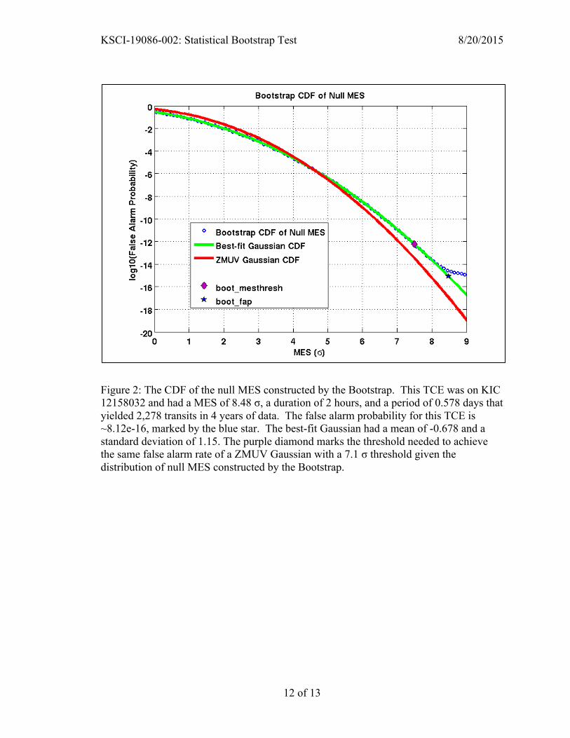
Figure 2 shows a typical bootstrap result. The TCE used for this plot was on KIC 12158032 and had a transit duration of 2 hours, an orbital period of 0.578 days, and a MES of 8.48 σ. If the MES of the detection falls below the MES corresponding to a log10(FAP) of -13.5, then the boot_fap is interpolated from the CDF of the null MES constructed by the Bootstrap, otherwise the best-fit Gaussian is used to calculate the boot_fap. In Figure 2 it is marked by the blue star and was calculated to be ~8.12e-16. This is the false alarm probability on the solid green curve corresponding to the MES of the TCE. The boot_mesthresh for this TCE is ~7.5 σ as can be seen by finding the MES corresponding to a false alarm probability of ~6.24e-13 on the best-fit Gaussian. In Figure 2 it is marked by the purple diamond. The boot_mesmean is the mean of the best-fit Gaussian and is -0.678 for this TCE. The boot_messtd is the standard deviation of the best-fit Gaussian and is 1.15 for this TCE. Note that the solid red curve shows the CDF for a Zero Mean Unit Variance (ZMUV) Gaussian. The fit of the best-fit Gaussian is done robustly in log space using the data from 1e-4 to 1e-13 to avoid the roll-off toward larger MES.


12 of 13

Figure 2: The CDF of the null MES constructed by the Bootstrap. This TCE was on KIC 12158032 and had a MES of 8.48 σ, a duration of 2 hours, and a period of 0.578 days that yielded 2,278 transits in 4 years of data. The false alarm probability for this TCE is ~8.12e-16, marked by the blue star. The best-fit Gaussian had a mean of -0.678 and a standard deviation of 1.15. The purple diamond marks the threshold needed to achieve the same false alarm rate of a ZMUV Gaussian with a 7.1 σ threshold given the distribution of null MES constructed by the Bootstrap.


13 of 13

5. References Jenkins, J. M. 2002, ApJ, 575, 493 Jenkins, J. M., Caldwell, D. A., & Borucki, W. J. 2002, ApJ, 564, 495 Jenkins, J. M., Chandrasekaran, H., McCauliff, S. D., et al. 2010, Proc SPIE, 7740, 77400D Jenkins, J.M., Twicken, J.D., Batalha, N.M., et al. 2015, Submitted to ApJ Seader, S., Tenenbaum, P., Jenkins, J. M., & Burke, C. J. 2013, ApJS, 206, 25 Seader, S., Jenkins, J. M., Tenenbaum, P., et al. 2015, ApJS, 217, 18 Tenenbaum, P., Jenkins, J. M., Seader, S., et al. 2014, ApJS, 211, 6

statistical bootstrap test - nasa exoplanet...

Documents