statistical and computational models for whole word morphology
TRANSCRIPT
Statistical and Computational Modelsfor Whole Word Morphology
Von der Fakultat fur Mathematik und Informatikder Universitat Leipzig angenommene
Dissertationzur Erlangung des akademischen GradesDoctor rerum naturalium
(Dr. rer. nat.)im Fachgebiet Informatik
vorgelegt vonMaciej Janicki, M. Sc.
geboren am 10.08.1989 in Wrocław, Polen
Die Annahme der Dissertation wurde empfohlen von:
1. Prof. Dr. Gerhard Heyer (Universitat Leipzig)
2. Prof. Dr. Uwe Quasthoff (Universitat Leipzig)
3. Dr. Krister Linden (Universitat Helsinki)
Die Verleihung des akademischen Grades erfolgt mit Bestehen derVerteidigung am 13. August 2019 mit dem Gesamtpradikat
magna cum laude.
brought to you by COREView metadata, citation and similar papers at core.ac.uk
provided by Qucosa - Publikationsserver der Universität Leipzig

ii
Abstract
The purpose of this thesis is to provide an unsupervised machine learning approachfor language morphology, in which the latter is modeled as string transformationson whole words, rather than the segmentation of words into smaller structuralunits.
The choice of a transformation-based morphology model is motivated mainlyby the realization that most Natural Language Processing methods treat wordsas basic units of language, and thus the application of morphological analysis isusually centered at describing relations between words, rather than processing sub-word units. On the other hand, segmentational approaches sometimes require an-swering questions that are both difficult and irrelevant for most applications, suchas whether to segment the German word fahig ‘able’ into fah-ig or the English sui-cide into sui-cide. Furthermore, non-concatenative phenomena like German umlautare not covered by segmentational approaches.
The whole-word-based model of morphology employed in this work is rootedin linguistic theories rejecting the notion of morpheme, particularly Whole WordMorphology. In this theory, it is words that are minimal elements of the languagecombining form and meaning. Morphology is expressed in terms of patterns de-scribing a regular interrelation in form and meaning within pairs of words. Suchformulation naturally results in a representation of the lexicon as a graph, in whichwords are vertices and pairs of words related via a productive, systematic patternare connected with an edge.
The contribution of the present thesis is twofold. Firstly, I provide a computa-tional model for Whole Word Morphology. Its foundation is a formal definition ofmorphological rule as a function mapping strings to sets of strings (as the applica-tion of a rule to a word may result in multiple outcomes or no outcome). The rulesare formulated in terms of patterns, which consist of alternating constant elements– describing parts of the word that are affected by the rule – and variable elements,
iii

iv
which stand for parts of the word unaffected by the rule. For example, the rulemapping the German word HausN.sg ‘house’ to HauserN.pl ‘houses’ has the form:/X1aX2/N.sg → /X1aX2er/N.pl, where X1 and X2 are variables, which can be in-stantiated with any string. The rules formulated this way can be easily expressedas Finite State Transducers, which enables us to use readily available, performantalgorithms for tasks like disjunction of rules or application of a rule to a word or setof words. For the task of rule induction, i.e. extracting rules from pairs of similarwords, I propose an approach based on modified versions of algorithms related toedit distance (Fast Similarity Search and the Wagner-Fischer algorithm).
Secondly, I propose a statistical model for graphs of word derivations. It isa generative model defining a joint probability distribution over the vertices andedges of the graph. The model is parameterized by a set of rules, as well as a vectorof numeric parameters, from which the probability of application of a particularrule to a particular word can be computed. Of the two inference problems for thismodel – fitting consisting of finding optimal values for the numeric parameters andmodel selection corresponding to selecting an optimal set of rules – especially fittingis considered in detail. It is realized by the Monte Carlo Expectation Maximizationalgorithm, which iteratively maximizes the expected log-likelihood of the graph.In order to approximate expected values over all possible configurations of graphedges, a sampler based on Metropolis-Hastings algorithm is developed.
Once trained, the model can be applied to a variety of tasks. The experimentspresented in the thesis include inducing lexemes (sets of word forms correspondingto the same lemma) by means of graph clustering, predicting new words to reduceout-of-vocabulary word rates and predicting part-of-speech tags for unknown wordsafter unsupervised training on a tagged dataset. Although developed for unsuper-vised training, the model can also be trained in a supervised setting, producingreasonable results in tasks like lemmatization or inflected form generation. How-ever, its main strength lies in a direct description and generalization of regularitiesamongst words encountered in unlabeled data, without referring to any linguisticnotion of ‘morphological structure’ or ‘analysis’.

Contents
1 Introduction 11.1 Theories of Morphology . . . . . . . . . . . . . . . . . . . . . . . . 2
1.1.1 Segmentational Morphology . . . . . . . . . . . . . . . . . . 31.1.2 Limitations of Segmentational Morphology . . . . . . . . . . 61.1.3 Word-Based Theories . . . . . . . . . . . . . . . . . . . . . . 9
1.2 Morphology in Natural Language Processing . . . . . . . . . . . . . 161.3 Goals and Contributions of This Thesis . . . . . . . . . . . . . . . . 20
2 A Review of Machine Learning Approaches to Morphology 232.1 Recognition of Morph Boundaries . . . . . . . . . . . . . . . . . . . 242.2 Grouping Morphologically Related Words . . . . . . . . . . . . . . . 272.3 Predicting the Properties of Unknown Words . . . . . . . . . . . . . 292.4 Discussion . . . . . . . . . . . . . . . . . . . . . . . . . . . . . . . . 31
3 Morphology as a System of String Transformations 333.1 Formalization of Morphological Rules . . . . . . . . . . . . . . . . . 333.2 Finite State Automata and Transducers . . . . . . . . . . . . . . . 36
3.2.1 Preliminaries . . . . . . . . . . . . . . . . . . . . . . . . . . 373.2.2 Compiling Morphological Rules to FSTs . . . . . . . . . . . 403.2.3 Binary Disjunction . . . . . . . . . . . . . . . . . . . . . . . 423.2.4 Computing the Number of Paths in an Acyclic FST . . . . . 453.2.5 Learning Probabilistic Automata . . . . . . . . . . . . . . . 47
3.3 Rule Extraction . . . . . . . . . . . . . . . . . . . . . . . . . . . . . 513.3.1 Finding Pairs of Similar Words . . . . . . . . . . . . . . . . 513.3.2 Extraction of Rules from Word Pairs . . . . . . . . . . . . . 543.3.3 Filtering the Graph . . . . . . . . . . . . . . . . . . . . . . . 613.3.4 Supervised and Restricted Variants . . . . . . . . . . . . . . 61
4 Statistical Modeling and Inference 634.1 Model Formulation . . . . . . . . . . . . . . . . . . . . . . . . . . . 63
4.1.1 The Basic Model . . . . . . . . . . . . . . . . . . . . . . . . 644.1.2 Distributions on Subsets of a Set . . . . . . . . . . . . . . . 654.1.3 Penalties on Tree Height . . . . . . . . . . . . . . . . . . . . 654.1.4 Part-of-Speech Tags . . . . . . . . . . . . . . . . . . . . . . 66
v

vi Contents
4.1.5 Numeric Features . . . . . . . . . . . . . . . . . . . . . . . . 674.2 Model Components . . . . . . . . . . . . . . . . . . . . . . . . . . . 68
4.2.1 Root Models . . . . . . . . . . . . . . . . . . . . . . . . . . . 694.2.2 Edge Models . . . . . . . . . . . . . . . . . . . . . . . . . . 704.2.3 Tag Models . . . . . . . . . . . . . . . . . . . . . . . . . . . 714.2.4 Frequency Models . . . . . . . . . . . . . . . . . . . . . . . . 724.2.5 Word Embedding Models . . . . . . . . . . . . . . . . . . . . 73
4.3 Inference . . . . . . . . . . . . . . . . . . . . . . . . . . . . . . . . . 754.3.1 MCMC Methods and the Metropolis-Hastings Algorithm . . 764.3.2 A MCMC Sampler for Morphology Graphs . . . . . . . . . . 794.3.3 Sampling Negative Examples . . . . . . . . . . . . . . . . . 834.3.4 Fitting the Model Parameters . . . . . . . . . . . . . . . . . 844.3.5 Model Selection . . . . . . . . . . . . . . . . . . . . . . . . . 864.3.6 Finding Optimal Branchings . . . . . . . . . . . . . . . . . . 87
5 Learning Inflectional Relations 895.1 Datasets . . . . . . . . . . . . . . . . . . . . . . . . . . . . . . . . . 905.2 Unsupervised Clustering of Inflected Forms . . . . . . . . . . . . . . 915.3 Unsupervised Lemmatization . . . . . . . . . . . . . . . . . . . . . 955.4 Supervised Lemmatization . . . . . . . . . . . . . . . . . . . . . . . 965.5 Supervised Inflected Form Generation . . . . . . . . . . . . . . . . . 99
6 Semi-Supervised Learning of POS Tagging 1036.1 A General Idea . . . . . . . . . . . . . . . . . . . . . . . . . . . . . 104
6.1.1 Intrinsic and Extrinsic Tag Guessing . . . . . . . . . . . . . 1046.1.2 Applying Tagged Rules to Untagged Words . . . . . . . . . 105
6.2 The Method . . . . . . . . . . . . . . . . . . . . . . . . . . . . . . . 1066.2.1 The Forward-Backward Algorithm for Trees . . . . . . . . . 1086.2.2 Modifications to the Sampling Algorithm . . . . . . . . . . . 1116.2.3 Extending an HMM with New Vocabulary . . . . . . . . . . 114
6.3 Evaluation . . . . . . . . . . . . . . . . . . . . . . . . . . . . . . . . 1156.3.1 Experiment Setup . . . . . . . . . . . . . . . . . . . . . . . . 1156.3.2 Evaluation Measures . . . . . . . . . . . . . . . . . . . . . . 1166.3.3 Results . . . . . . . . . . . . . . . . . . . . . . . . . . . . . . 1176.3.4 Remarks . . . . . . . . . . . . . . . . . . . . . . . . . . . . . 120
7 Unsupervised Vocabulary Expansion 1237.1 Related Work . . . . . . . . . . . . . . . . . . . . . . . . . . . . . . 1247.2 The Method . . . . . . . . . . . . . . . . . . . . . . . . . . . . . . . 124
7.2.1 Predicting Word Frequency . . . . . . . . . . . . . . . . . . 1257.2.2 Computing Word Costs from Edge Probabilities . . . . . . . 126
7.3 Evaluation . . . . . . . . . . . . . . . . . . . . . . . . . . . . . . . . 1287.3.1 Experiment Setup . . . . . . . . . . . . . . . . . . . . . . . . 1287.3.2 Results . . . . . . . . . . . . . . . . . . . . . . . . . . . . . . 129

Contents vii
8 Conclusion 137
Bibliography 141

viii Contents

List of Figures
1.1 An example analysis of relied in two-level morphology. . . . . . . . 171.2 A typical segmentational analysis of the German word beziehung-
sunfahiger. The information contained in the inner nodes (shown ingray) is lost in the segmentation. . . . . . . . . . . . . . . . . . . . 18
3.1 A scheme for converting morphological rules into FSTs. . . . . . . . 413.2 The transducer corresponding to rule (3.3). . . . . . . . . . . . . . . 413.3 The transducer corresponding to rule (3.9). . . . . . . . . . . . . . . 413.4 A comparison of running times for different disjunction strategies. . 443.5 The transducer S1 for generating a deletion neighborhood. . . . . . 523.6 The filter S2 ensuring, that no more than the half of a word is deleted. 533.7 Matrices D, Ξ, X, Y and aligned sequences u, v after executing Al-
gorithm 3.8 on the word pair (trifft, getroffen). The shaded cellscorrespond to the optimal alignment, which is extracted by Algo-rithm 3.9. . . . . . . . . . . . . . . . . . . . . . . . . . . . . . . . . 56
3.8 Rules extracted from the pair (trifft, getroffen) by Algorithm 3.10and their corresponding masks, sorted by generality. . . . . . . . . . 59
4.1 An example tree of word derivations. . . . . . . . . . . . . . . . . . 644.2 A ‘bad’ tree caused by the lack of a constraint on tree height. . . . 664.3 NN architecture for the edge model. . . . . . . . . . . . . . . . . . . 714.4 NN architecture for the root tag model. . . . . . . . . . . . . . . . . 724.5 The difference in log-frequencies between words on the left and right
side of the rule /Xen/→ /Xes/ in German. The dashed line is thebest-fitting Gaussian density. . . . . . . . . . . . . . . . . . . . . . . 73
4.6 NN architecture for the root vector model. . . . . . . . . . . . . . . 744.7 NN architecture for the edge vector model. . . . . . . . . . . . . . . 754.8 The two variants of the ‘flip’ move. The deleted edges are dashed
and the newly added edges dotted. The goal of the operation is tomake possible adding an edge from v1 to v2 without creating a cycle. 80
4.9 The trajectory of the graph sampler expressed as the cost (negativelog-likelihood) of the graph at a given iteration. The top plot showsall 10 million sampling iterations, while the bottom plot shows iter-ations from 4 million onward. The acceptance rate in this run was0.12. . . . . . . . . . . . . . . . . . . . . . . . . . . . . . . . . . . . 82
ix

x List of Figures
4.10 Convergence of MCEM fitting. The cost at the first iteration is farbeyond the scale (around 1.6 · 106). . . . . . . . . . . . . . . . . . . 86
4.11 The number of rules and possible edges during model selection. . . 88
6.1 Two possible morphology graphs corresponding to the words machen,mache, macht. What does each of them tell us about the possibletags of those words according to (6.1)? . . . . . . . . . . . . . . . . 106
6.2 The Forward-Backward computation for a linear sequence in anHMM. αv6,t = P (v1, . . . , v6, T6 = t), whereas βv6,t = P (v7, v8, v9|T6 =t). . . . . . . . . . . . . . . . . . . . . . . . . . . . . . . . . . . . . 108
6.3 The Forward-Backward computation for a tree. Also here, αv6,t =P (v1, . . . , v6, T6 = t) and βv6,t = P (v7, v8, v9|T6 = t). . . . . . . . . . 109
6.4 Adding or removing the edge (v, v′, r). . . . . . . . . . . . . . . . . 1126.5 Exchanging an edge to another with the same target node. The
change can take place within one tree (a) or involve two separatetrees (b). . . . . . . . . . . . . . . . . . . . . . . . . . . . . . . . . . 113
6.6 In case of a ‘flip’ move, the smallest subtree containing all changesis the one rooted in v3. The deleted edges are dashed, while thenewly added edges are dotted. In order to obtain the new βv3 , werecompute the backward probabilities in the whole subtree. αv3 isnot affected by the changes. (The node labels are consistent withthe definition in Fig. 4.8.) . . . . . . . . . . . . . . . . . . . . . . . 113
6.7 A special case of the ‘flip’ move, which changes the root of the tree.(a) – the tree before the move (the edge to delete is dashed, whilethe edge to be added is dotted); (b) – the tree after the move. Thenode labels agree with the ones in Fig. 4.8, with v4 = v2, v5 = v1
and v3 not existing. The difference between the two variants of ‘flip’is neutralized in this case. . . . . . . . . . . . . . . . . . . . . . . . 113
7.1 Predicted log-frequency of the hypothetical word *jedsten, as de-rived from jedes via the rule /Xes/ → /Xsten/. The frequencymodel predicts the mean log-frequency µ = 4.24 (correspondingto the frequency around 69) with standard deviation σ = 0.457.The probability of the word not occurring in the corpus (i.e. fre-quency < 1) corresponds to the area under the curve on the interval(−∞, 0), which is approximately 10−20. . . . . . . . . . . . . . . . 125
7.2 Predicted log-frequency of aufwandigsten, as derived from aufwandigesvia the rule /Xes/→ /Xsten/. The probability of log-frequency be-ing negative (i.e. the frequency being < 1) is here around 0.863(µ = −0.5, σ = 0.457). . . . . . . . . . . . . . . . . . . . . . . . . . 126
List of Tables
3.1 Commonly used semirings. ⊕log is defined by: x⊕log y = − log(e−x+e−y). . . . . . . . . . . . . . . . . . . . . . . . . . . . . . . . . . . . 38
3.2 Example rules extracted from the German Wikipedia. . . . . . . . . 60
5.1 Results of unsupervised clustering. . . . . . . . . . . . . . . . . . . 945.2 Results of unsupervised lemmatization. . . . . . . . . . . . . . . . . 975.3 Size (number of types) of the datasets used for supervised lemmati-
zation. . . . . . . . . . . . . . . . . . . . . . . . . . . . . . . . . . . 975.4 Results of supervised lemmatization. . . . . . . . . . . . . . . . . . 1005.5 Results of supervised inflected form generation. . . . . . . . . . . . 101
6.1 Different setups of the HMM tagger used in the tagging experiment. 1166.2 Lexicon evaluation with coarse-grained tags. . . . . . . . . . . . . . 1186.3 Lexicon evaluation with fine-grained tags. . . . . . . . . . . . . . . 1186.4 Tagging evaluation with coarse-grained tags. . . . . . . . . . . . . . 1196.5 Tagging evaluation with fine-grained tags. . . . . . . . . . . . . . . 120
7.1 The datasets used for evaluation. . . . . . . . . . . . . . . . . . . . 1297.2 Token-based OOV reduction rates for various numbers of generated
words. . . . . . . . . . . . . . . . . . . . . . . . . . . . . . . . . . . 1307.3 Type-based OOV reduction rates for various numbers of generated
words. . . . . . . . . . . . . . . . . . . . . . . . . . . . . . . . . . . 1317.4 Type-based OOV reduction as the percentage of the maximal re-
duction at a given size. . . . . . . . . . . . . . . . . . . . . . . . . . 134
xi

xii List of Tables

List of Algorithms
3.1 Binary disjunction. . . . . . . . . . . . . . . . . . . . . . . . . . . . . 433.2 Computing the number of paths in an acyclic DFST. . . . . . . . . . 463.3 STOCHASTIC-MERGE. . . . . . . . . . . . . . . . . . . . . . . . . 483.4 STOCHASTIC-FOLD. . . . . . . . . . . . . . . . . . . . . . . . . . . 493.5 ALERGIA-TEST. . . . . . . . . . . . . . . . . . . . . . . . . . . . . 493.6 ALERGIA-COMPATIBLE. . . . . . . . . . . . . . . . . . . . . . . . 503.7 ALERGIA. . . . . . . . . . . . . . . . . . . . . . . . . . . . . . . . . 503.8 Aligning similar words with minimum number of edit operations. . . 553.9 Extract-alignment. . . . . . . . . . . . . . . . . . . . . . . . . . 553.10 Extracting rule candidates from pairs of similar words. . . . . . . . . 58
4.1 A single iteration of the Metropolis-Hastings algorithm. . . . . . . . 794.2 Proposing the next branching in the sample. . . . . . . . . . . . . . . 814.3 Sampling negative examples of edges. . . . . . . . . . . . . . . . . . . 84
xiii

xiv List of Algorithms
Acknowledgments
As is the case with every dissertation, also this one would not have been possiblewithout support and good will of many people. First and foremost, I would like tothank my supervisors, Prof. Uwe Quasthoff and Prof. Gerhard Heyer. While theyalways supported me with advice and feedback, they also gave me a tremendousamount of freedom and trust in pursuing my own ideas. Furthermore, they securedthe financial resources, including a three-year scholarship, which gave me a plentyof time to work on this topic. I also thank my colleagues, especially Dr. IngmarSchuster, Max Bryan and Dr. Christoph Teichmann, for valuable discussions andintroducing me to some topics, notably neural networks and Markov Chain MonteCarlo. I thank Dr. Giuseppe G. A. Celano for the consultation on Latin and AncientGreek, as well as Christopher Schroder for proofreading. Finally, I thank all thecolleagues that have worked in the office P818 over the years for contributing to afriendly and productive work environment.
This thesis was completed entirely using free software. The methods describedhere were implemented in Python. All the work was done under GNU/Linux sys-tems and the text was typeset using LATEX. I could not imagine efficient workwithout tools like the various tiling window managers or the Vim text editor. Iowe much to the free software community. As to the more specialized software, Iwould like to thank the developers of OpenFST, HFST and Keras for their excellentwork.
I also thank Michał Śliwiński, a teacher from my high school, for introduc-ing me to the International Linguistics Olympiad and awakening my interest intheoretical and computational linguistics, which has shaped my whole professionalcareer. Further thanks to the rock band Linie 7ieben, of which I was a member forthe past 4 years, for providing me with pleasant distraction and a tempting careeralternative.
The period of work on this thesis saw a wedding, as well as an abrupt breakupof the marriage two years later. I am deeply grateful to all the people who supported
xv

xvi Acknowledgments
me through 2018, which was the most difficult year of my life. I particularly wantto mention my parents Anna and Andrzej, my brother Marek, and my friends fromLeipzig: Agata Barcik, Basia Kubaińska and Cyprian Zajt. Needless to say, theywere great company in better times as well.

Chapter 1
Introduction
Every good work of software starts by
scratching a developer’s personal itch.Eric Raymond, The Cathedral and the Bazaar
This thesis is concerned with the topic of machine learning of language mor-phology. The focus lies on unsupervised learning, i.e. learning from raw, observablelanguage data, without any additional labeling. This contrasts with supervisedlearning, i.e. learning from data labeled by human experts, as well as rule-basedapproaches, in which the language processing relies on manually constructed re-sources, like dictionaries and grammars. While the early history of Natural Lan-guage Processing (NLP) was dominated by rule-based approaches grounded in for-mal linguistic theories, the recent two or three decades have seen a nearly completeshift towards machine learning methods.
Despite their relatively low reliability (as compared to the two other ap-proaches), unsupervised language learning methods have been a topic of active re-search for the entire history of NLP. Their roots lie in the linguistic structuralismof the early 20th century, which placed emphasis on deriving grammatical notionsdirectly from observable language data. Concrete algorithms were presented as farback as 1950s [Harris 1955]. More recently, the rise of shared tasks like MultilingualParsing from Raw Text to Universal Dependencies [Hajic and Zeman 2017] atteststhe increasing practical significance of unsupervised methods and high expectationsplaced on them by the research community.
In addition to the practical benefits of unsupervised learning, like rapid adap-tation to new languages and domains, or the possibility of processing resource-scarce languages, for which human experts are unavailable, the research on un-supervised methods also poses interesting theoretical questions. An unsupervised
1

2 Chapter 1. Introduction
learning algorithm is expected to derive a knowledge representation from unanno-tated data, without any clue from a human annotator about what kind of represen-tation is expected – apart from the clues contained in the design of the algorithmitself, in isolation from the data. Therefore, unsupervised learning requires an es-pecially careful consideration of what should be learnt and how it can be derivedfrom observable data. It thus stimulates the research on finding plausible repre-sentations of linguistic knowledge which are as near to electronically available,machine-readable language data as possible.1 Furthermore, it might also shed lighton the process of first language acquisition by humans, which is similar (althoughnot entirely analogical) to unsupervised learning.
Correspondingly, the thesis begins by addressing the question of what repre-sentation should be learnt and how it relates to observable data. In Section 1.1, Ireview different approaches to morphology found in theoretical linguistics. Section1.2 describes how those theories are applied to derive representations of morphol-ogy used in NLP and what kinds of morphological analysis are expected in practicalapplications. It turns out that the widely adopted segmentational view suffers fromdiscrepancies: both between its strictly concatenative model of morphology and thereality of morphological phenomena, and between its objective and the use casesfor morphological analysis in NLP. Those considerations lead to the motivation forthe current thesis, which is adapting for the purposes of NLP an apparently un-derexplored and promising theory which takes a relational (rather than structural)view on morphology. This goal is elaborated in Sec. 1.3.
1.1 Theories of Morphology
Morphology is the part of language grammar concerned with individual words. Asexplained by an introductory text (emphasis original):
In linguistics morphology refers to the mental system involved inword formation or to the branch of linguistics that deals with words,their internal structure and how they are formed.
[Aronoff and Fudeman 2004, p. 2]
Morphology is usually divided into inflection, derivation and compounding,which are treated differently by many theories. However, it is difficult to formulate1For example, the research on unsupervised parsing, as well as machine learning of parsing
in general, recently contributed to the wide popularity of dependency grammar in the NLPcommunity.

1.1. Theories of Morphology 3
a clear definition distinguishing inflection from derivation. In a commonly used un-derstanding, inflection is responsible for providing the word with features requiredby the syntactic context (like e.g. case or number), whereas derivation forms newwords with new meanings. The term compounding is used for the process of creatinga new word from more than one base word (like lighthouse ← light + house).
The above quote of Aronoff and Fudeman mentions two subjects: the internalstructure of words and the process of word formation. A view shared by a largemajority (but not all) of grammar theorists is that a theory of morphology issupposed to describe both of them and that the process of word formation istightly related to the internal word structure. The latter is usually described interms of morphemes, which constitute the basic building blocks for words. Some ofthe most influential theories based on this assumption are described in Sec. 1.1.1.
Although the assumption of internal word structure seems intuitive, thereare certain phenomena in morphology which are very difficult to describe this way.Extending the basic theory to account for such cases results in a very abstract andvaguely defined notion of morpheme, which is only remotely related to the originalidea. In Sec. 1.1.2, we look into details of such problems and how they are typicallyhandled.
Finally, in Sec. 1.1.3, we turn to different theories of morphology, which makelittle or no assumptions about the internal structure of words and instead focusentirely on the process of word formation or structural similarities between words.Such theories provide the motivation and linguistic foundation for the currentthesis.
1.1.1 Segmentational Morphology
The concept of a word being composed out of smaller, meaning-bearing units datesback to the ancient Indian grammar tradition, especially to Pan. ini’s grammar ofSanskrit [Gillon 2007]. In contrast, the older European grammar tradition con-centrated on the study of words and paradigms, treating words as basic unitsof meaning. The notion of morpheme as a minimal meaningful unit of languagewas popularized by the American structuralist school in the first half of the 20thcentury in the following formulation:
A linguistic form which bears no partial phonetic-semantic resem-blance to any other form, is a simple form or morpheme.
[Bloomfield 1933, p. 161]

4 Chapter 1. Introduction
This definition is part of the structuralist approach to language. The struc-turalist school aimed to derive linguistic descriptions strictly from the structuralproperties of language. The most important criterion was the distribution of variouselements of the language and its influence on the meaning. Contrary to older tra-ditions, the structuralist school put emphasis on the spoken language, rather thanwritten, as the subject of linguistic analysis [Bloomfield 1933, p. 21]. The struc-turalist approach to morphology was further elaborated in works such as [Nida1949] and [Harris 1951].
Later interpretations of the above definition state that morphemes are min-imal signs of the language. The notion of sign, introduced by de Saussure [1916],is essential in structuralist linguistics. A sign is an entity consisting of form andmeaning, in which the connection between the two is arbitrary, i.e. one cannotbe predicted from the other. Language is thus a system of signs, as every spokenutterance has a meaning, which is related to its phonetic form only by means ofthe convention of a particular language.
The usefulness of morphemes as means of predicting the relationship betweenform and meaning of words can be illustrated by the following example:
Example 1.1. Finnishlentokoneissanikin
lento kone i ssa ni kinflight machine pl iness 1sg too
‘in my aeroplanes, too’
It is not very likely for a Finnish speaker to ever have heard exactly this word.2
After all, hardly anybody possesses multiple aeroplanes. However, understandingit will not pose any problems to the speaker, because it contains parts knownfrom many other words, like -i- (plural), -ssa ‘in’, -ni ‘my’ (possessive suffix) and-kin ‘too’. Even the word lentokone ‘aeroplane’, which is probably known to allFinnish speakers, is composed in a transparent way, so that one could understandit without having heard it before.
It can be seen from Example 1.1 that Finnish morphology is (mostly) agglu-tinative: each unit of meaning or grammatical function corresponds to one mor-pheme. The morphemes are concatenated to form words. On the other hand, wespeak of fusional morphology if multiple grammatical functions are fused in a sin-gle morpheme. For example, the Polish equivalent of ‘in planes’ is w samolotach,
2A Web search with DuckDuckGo finds no results for this word. (accessed on Jan 16, 2019)

1.1. Theories of Morphology 5
where the suffix -ach contains both ‘plural’ and ‘locative’ features, which cannotbe isolated. Languages with fusional morphology typically display fewer morphsper word, more homophony of functional morphemes (called syncretism) and morenon-concatenative phenomena.
The two fundamental models of morphology that emerged in the mid-20th cen-tury were the Item-and-Arrangement (IA) and the Item-and-Process (IP) model[Hockett 1954]. Especially the former is tightly related to the notion of morpheme:words (and ultimately, all linguistic constructions) are arrangements of morphemes.The arrangement encompasses more than just the linear ordering: also a kind ofconstituent structure is postulated. Morphology in this formulation is thus some-what similar to syntax, but operating below the word level. This analogy has beenexplored in more detail by, among others, Selkirk [1982].
In a simplified view, the IA model could be characterized as follows:
w = µ1µ2 . . . µk (1.1)
In this formulation, a word w is simply a sequence of morphemes µi. Themorphemes are realized by strings of phonemes called morphs and the concatena-tion operation is realized by grammar-wide morphophonological rules, which canchange the shape of morphs depending on their context. In order to account forthe hierarchical structure, one could additionally introduce a bracketing on thesequence of morphemes. Note that, in general, morphs are not allowed to con-tain any additional phonological information besides the string of phonemes (e.g.‘alternation markers’).
The IA model is a static description: it concentrates on identifying and de-scribing the internal structure of words. The regular similarity in form and meaningof words can then be explained by the common elements of the internal structure.
On the other hand, the Item-and-Process model describes the structure ofwords in dynamic terms: words are derived from other words (or from more ab-stract lexical items, like stems or roots) by means of processes. This model may, butdoes not have to, involve the notion of morpheme. However, there is a widespreadagreement that a process typically encompasses adding some phonological mate-rial, called process markers. The naming of some processes, like affixation (i.e. theaddition of an affix) indicates though, that morphemes are implicitly present inmost IP descriptions as well.
A schematic formulation of the IP model, analogously to (1.1), would thus

6 Chapter 1. Introduction
be the following:w = πk(πk−1(. . . π1(r) . . .)) (1.2)
A word w is derived from a root r through a series of processes πi, each ofwhich takes the output of the previous process as its input. In contrast to the IAmodel, in which everything was a morpheme, the roots and the processes in the IPmodel are fundamentally different entities.
The main problem with the IP model is that it is very difficult to define whatexactly a process may and may not do. Allowing arbitrary rewrite rules is clearlytoo strong, while restricting the processes to addition of phonological material isclearly too weak. Besides, it is not clear what exactly is the input of a process.In addition to complete existing words, ‘incomplete words’ (stems) are normallyallowed and it is difficult to define such entities precisely, as well as prove thatlanguage speakers possess an internal representation of them.
1.1.2 Limitations of Segmentational Morphology
While the intuition that stands behind the notion of morpheme is clearly seen ina case like Example 1.1, there are many kinds of similarities between words thatcannot be easily analyzed using morphemes. This usually leads to workaroundsand extensions to the basic theory: in case of the IA model, either the morphs areallowed to contain abstract, transformation-related information (which, as [Hockett1954, p. 224] points out, undermines the whole idea of Item-and-Arrangement),or too much burden is put on morphophonological rules, which are expected to‘fix’ the discrepancy between the model and the reality. In case of the IP model,the flexible notion of ‘process’ is used to encompass more and more sophisticatedtransformations. In both cases, the result is a, in my opinion, vague theory withunclearly defined concepts.
In the following, I present a few fairly common phenomena, which pose prob-lems for segmentational morphology, as well as for NLP applications built upon asegmentational theory of morphology.
Stem alternation. Stem alternation is probably the most common non-conca-tenative phenomenon in morphology: a certain sound inside the stem (often thestressed vowel) undergoes a regular transformation. Example 1.2 shows German

1.1. Theories of Morphology 7
plural formation which exhibits the well-known umlaut.
Example 1.2. Germana. Haus /haU
“s/ ‘house.nom.sg’
Hauser /hOY“z5/ ‘house.nom.pl’
b. Buch /bu:x/ ‘book.nom.sg’Bucher /by:ç5/ ‘book.nom.pl’
c. Vater /fA:t5/ ‘father.nom.sg’Vater /fE:t5/ ‘father.nom.pl’
Sound changes at morph boundaries. Some affixes trigger sound changes af-fecting the nearby phonemes. It is unclear whether the resulting alternation shouldbe modeled as part of the affix or as stem alternation. In Example 1.3, -a is thenominative suffix of many Polish feminine nouns. The locative suffix is somethinglike -je, where the first element triggers a regular consonant change. (Note thatit is not even exactly a palatalization marker in the phonological sense, since thesequences /kje/ and /gje/ are possible in Polish.) It is difficult to mark morphboundaries here, as, strictly speaking, a part of the stem and a part of the suffixmelt into a single phoneme.
Example 1.3. Polisha. droga /drOga/ ‘way-nom.sg’
drodze /drO>dzE/ ‘way-loc.sg’
b. ręka /rENka/ ‘hand-nom.sg’ręce /rEn
>tsE/ ‘hand-loc.sg’
c. strata /strata/ ‘loss-nom.sg’stracie /stra
>tCe/ ‘loss-loc.sg’
d. woda /vOda/ ‘water-nom.sg’wodzie /vO
>dýe/ ‘water-loc.sg’
e. zupa /zupa/ ‘soup-nom.sg’zupie /zupje/ ‘soup-loc.sg’
f. żaba /Zaba/ ‘frog-nom.sg’żabie /Zabje/ ‘frog-loc.sg’
Zero morphs. It is often convenient to tie some grammatical categories, like e.g.plural, to a particular morpheme that occurs in the respective form. In Example1.4b, the ‘plural’ feature is associated with the suffix -s, while the stem housedoes not carry any number feature. In case of 1.4a, the word consists of only

8 Chapter 1. Introduction
one morpheme, which is supposed to be the same stem as in 1.4b. However, theword also contains the feature ‘singular’, which would have to be located in thisonly morpheme. There are two possible conclusions for the segmentational analysis:either the stems in 1.4a and 1.4b are homophonic, but distinct morphemes, one withthe singular feature and one without (which seems absurd), or the widely acceptedstatement that the word from 1.4a contains another morpheme: a ‘singular suffix’with null phonological realization.3 Many analyses tend to the latter option, thusallowing phonologically null morphs.
Example 1.4. Englisha. house ‘house.sg’b. house-s ‘house-pl’
Cranberry morphs. The term ‘cranberry morph’ was coined by Aronoff [1976].It describes a morph that occurs only in one word, like the first part of words inExample 1.5a. The rationale behind isolating such morphs is dubious, because nowell-defined meaning can be attributed to them – their meaning is inseparably tiedto the meaning of the word they occur in. For example, the only statement thatcan be made about the meaning of cran- is that it turns a generic berry into acranberry. However, berry is clearly a morph, as can be seen from the words listedin 1.5b.
Example 1.5. Englisha. cranberry boysenberry huckleberryb. strawberry blueberry blackberry gooseberry
[Aronoff 1976, p. 10]
Case studies like that of Rainer [2003], who analyzes in detail the Spanishderivational suffix -azo, show that attributing meanings to derivational affixes isdifficult as well. Instead, he suggests to treat meaning as a property of word. Themeaning of newly coined words is attributed by analogy to one or more alreadyexisting words derived with the same affix. However, the general meaning of anaffix does not have to be specified and once the words are coined, their meaningmay evolve in an idiosyncratic way.
3In fact, there are more possible explanations: for example that the plural feature overridesthe singular. While it seems to be a plausible explanation of the example, it is very difficult toconvert it into a general principle: what is overridden by what, why and when? Is the singularfeature part of the stem or is it assigned as default if no number is explicitly marked? As each ofsuch explanations raises further questions, the notion of ‘zero morph’ is widespread.

1.1. Theories of Morphology 9
Words of foreign origin. A frequent source of borderline cases for segmentationare borrowings, in which some morphological structure of the source language isstill visible. This is well exemplified by words of Greek and Latin origin in manyEuropean languages, especially English. Example 1.6a shows words that must havebeen borrowed into English already as compounds, as their first part is not a properEnglish morpheme. 1.6b lists words that correspond to valid Latin compounds,but might be English word formations as well. Finally, the words listed in 1.6care clearly English formations, demonstrating that the suffix -cide is productive inEnglish.4 Any consistent segmentation of all three groups is going to be disputable.
Example 1.6. Englisha. — deicide
— regicide— suicide
b. bacterium bactericideherb herbicideinfant infanticide
c. computer computerciderobot roboticidesquirrel squirrelcideweed weedicide
The examples presented in this section are only a modest selection of ‘prob-lematic’ phenomena. In my opinion, those pose the most problems for automaticprocessing, at least of European languages, which are the focus of this thesis. Fur-ther such phenomena include e.g. subtraction, reduplication, transfixation or mor-phologically conditioned stress and tone alternations. They are covered in detail inlinguistic literature, especially introductory works like [Aronoff and Fudeman 2004]or monographies critical of the notion of morpheme reviewed in the next section.
1.1.3 Word-Based Theories
The problems with the notion of morpheme are well-known in theoretical linguis-tics. To my knowledge, the first thorough critique of morpheme as a ‘minimalmeaningful unit’, combined with a theory of morphology based on rewrite rules,
4For references to sources attesting the words computercide, roboticide and squirrelcide, seethe Wiktionary pages for those words (accessed on Jan 11, 2019).

10 Chapter 1. Introduction
was proposed by Aronoff [1976]. It is rooted in the tradition of Generative Gram-mar and builds upon the treatment of morphology of, among others, Chomsky[1970] and Halle [1973].
After reviewing problems with the notion of morpheme as a minimal sign,especially ‘cranberry morphs’, Aronoff postulates a word-based theory of morphol-ogy by formulating a very important principle, which will apply to other theoriesas well:
Hypothesis: All regular word-formation processes are word-based.A new word is formed by applying a regular rule to a single alreadyexisting word. [. . . ]
[Aronoff 1976, p. 21]
Thus, rules are always applied to already existing words. However, Aronoff’s theoryis only concerned with word formation (i.e. derivation), as it views inflection to bea part of syntax. Correspondingly, what is referred to as ‘word’ is in fact ‘wordminus inflectional markers’. Moreover, despite the criticism, Aronoff upholds theconcept of morpheme as motivated, albeit not essential for a theory of morphologyand under a different, extremely vague, definition:
A morpheme is a phonetic string which can be connected to a lin-guistic entity outside that string.
[Aronoff 1976, p. 15]
Aronoff [2007] reiterates his criticism of the decomposition of morphologically com-plex words and provides arguments showing that complex words are usually lexi-calized and their meaning cannot be predicted from their postulated structure.
Another theory rejecting the notion of morpheme which is rooted in Genera-tive Grammar is A-morphous Morphology [Anderson 1992]. It views lexicon asconsisting of stems, which are again defined as ‘word minus inflectional material’.Inflection and derivation are treated as fundamentally different phenomena: whileinflection is thought of as part of syntax, derivation operates inside the lexicon.Those phenomena are realized by two kinds of rewrite rules: Word Formation Rulesgenerate words (inflected forms) from stems and constraints on morphosyntacticfeatures provided by the syntactic structure, whereas Stem Formation Rules gen-erate stems from other stems and exchange no information with the syntax. Thenotion of morpheme is explicitly rejected. Moreover, it is emphasized that both
1.1. Theories of Morphology 11
kinds of rules create no internal word structure which would be available to otherparts of grammar. However, in the analysis of compounding, Anderson makes someconcessions towards segmentational morphology (which are reviewed and criticizedin detail by Starosta [2003]).
The notion of morpheme and internal word structure continues to be a topicof debate in more recent research. Hay and Baayen [2005] provide a comprehen-sive overview of the discussion. They take an interesting intermediary position:while internal word structure is motivated, it is best seen as a gradient (i.e. fuzzy)structure, rather than discrete. This in turn fits into the larger-scale idea of incor-porating the notions of probability, uncertainty and fuzziness into grammar theory,which is comprehensively presented by [Bod et al. 2003].
Hudson [1984] proposes a theory named Word Grammar, which accounts forall major levels of linguistic representation (i.e. phonology, morphology, syntaxand semantics). Although it takes a concatenative, Item-and-Arrangement viewon morphology, it is interesting here for a different reason. Firstly, it displays anapproach that came to be called pan-lexicalism: all information relevant for produc-ing valid utterances of the language is stored in the lexicon. There is no ontologicaldistinction between lexical entries and rules : rules (e.g. of syntax) are also modeledas lexical entries. Secondly, the lexicon (together with all the grammatical infor-mation) is modeled as a network (i.e. graph), which, according to Hudson, is partof an even larger ‘cognitive network’. Both ideas – pan-lexicalism and the repre-sentation of lexicon as a graph – are fundamental to the theories of morphologypresented further below and to the model of morphology adopted by this thesis.
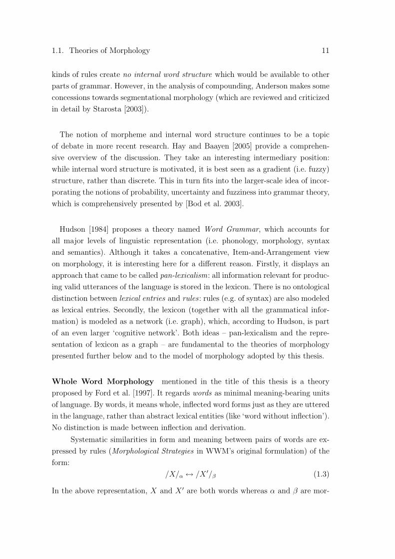
Whole Word Morphology mentioned in the title of this thesis is a theoryproposed by Ford et al. [1997]. It regards words as minimal meaning-bearing unitsof language. By words, it means whole, inflected word forms just as they are utteredin the language, rather than abstract lexical entities (like ‘word without inflection’).No distinction is made between inflection and derivation.
Systematic similarities in form and meaning between pairs of words are ex-pressed by rules (Morphological Strategies in WWM’s original formulation) of theform:
/X/α ↔ /X ′/β (1.3)
In the above representation, X and X ′ are both words whereas α and β are mor-

12 Chapter 1. Introduction
phosyntactic categories (‘part-of-speech tags’ in the language of NLP). The bidi-rectional arrow expresses that if a word fitting to the pattern on the left side ofthe rule exists, then the existence of a counterpart matching the right side is pos-tulated, and vice versa. The rule has no privileged direction and none of the wordsis said to be ‘derived’ from the other or morphologically ‘more complex’ than theother.
An example rule reflecting the relationship between French masculine andfeminine nouns like (chanteur, chanteuse) is expressed as follows:5
/Xœr/N.masc ↔ /Xøz/N.fem (1.4)
Thus, WWM provides a different answer to the fundamental question ‘whatis morphology?’:
Morphology is the study of formal relationships amongst words.
[Ford et al. 1997, p. 1]
The internal structure of words is not a subject of study here.A theory very similar to WWM was proposed as part of a larger theory of
dependency grammar called Lexicase [Starosta 1988]. The similarity was noted bythe authors of both theories, which resulted in a jointly edited volume [Singh andStarosta 2003], in which the common theory was renamed to Seamless Morphology.Starosta frequently cites Hudson and pan-lexicalism as an inspiration for his theory,which can also be seen as pan-lexicalist. In Lexicase syntax, there are no rules ofsyntax separate from the lexicon. Instead, the information about how words can becombined to form utterances is contained in the lexical entries: each word containsa frame of possible dependents (in the sense of dependency grammar).6 Rules like‘every noun can have an adjective dependent on its left’ emerge only as a methodof ‘compression’: to store redundant information efficiently, so that it does nothave to be memorized explicitly in every entry. The rules are thus not necessaryfor the functioning of the grammar and what exactly is covered by rules might beleft unclear. Starosta argues that the pan-lexicalist formulation is a more accuratemodel of human language processing than the traditional generative grammar:5The presentation given here follows exactly the one of [Ford et al. 1997]. In my opinion, it is
slightly misleading: X seems to have different meanings in (1.3) and in (1.4). Nevertheless, theintended meaning is apprehensible, at least from the example. My own version of the definitionof rule is given in Sec. 3.1.6This can be seen as an extreme counterpart of generative Phrase Structure Grammar, in
which the lexicon is contained in the grammar in form of rules generating terminals from non-terminals.

1.1. Theories of Morphology 13
[Psychological experiments] indicate that memory is far more im-portant in actual speech processing than most generative grammarianshad hitherto believed possible and the lexicon bears a much greaterburden in this respect than the rules which many of us have dedicatedour professional lives to constructing.
[Starosta 1988, p. 41]
The same approach is applied to morphology: although every word could bestored in the lexicon as a separate entry, it is more efficient to capture regularitiesin form of rules, which generate words from other words. The rules are formulatedvery similarly to those in WWM.
Compounding
Although compounding might seem to be the most articulate example of the con-catenative character of morphology, the authors of WWM make important pointsthere as well. An analysis of compounding as putting two words together to format third one, like (1.5), is rejected:
/X/+ /Y/↔ /XY/ (1.5)
Instead, the authors note that compounds come in clusters, in which at least oneof the parts is known from multiple compounds:
Facts of ‘compounding’ from various languages indicate quite clearlythat ‘compounds’ come in sets, each set anchored in some specific con-stant.
[Singh and Dasgupta 2003, p. 78]
A word that is not generally known as ‘compound-forming’ is unlikely to forma compound, even if there seems to be no reason to prevent it. This phenomenon
14 Chapter 1. Introduction
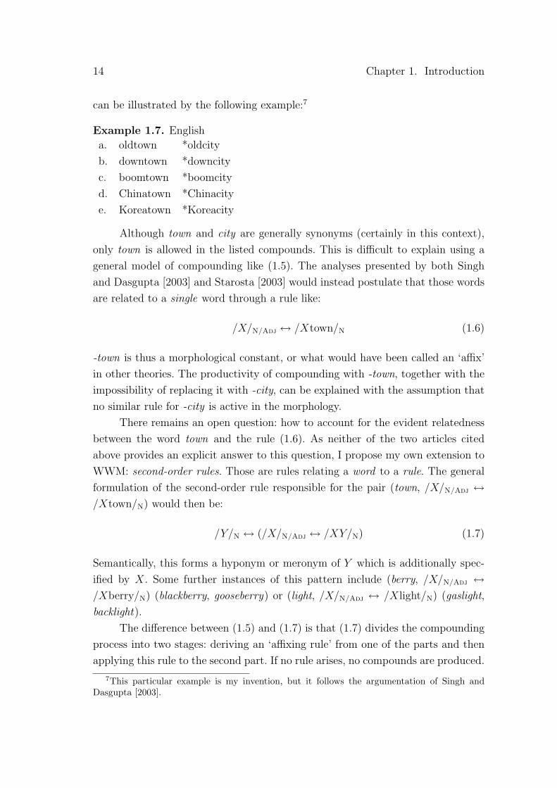
can be illustrated by the following example:7
Example 1.7. Englisha. oldtown *oldcityb. downtown *downcityc. boomtown *boomcityd. Chinatown *Chinacitye. Koreatown *Koreacity
Although town and city are generally synonyms (certainly in this context),only town is allowed in the listed compounds. This is difficult to explain using ageneral model of compounding like (1.5). The analyses presented by both Singhand Dasgupta [2003] and Starosta [2003] would instead postulate that those wordsare related to a single word through a rule like:
/X/N/Adj ↔ /Xtown/N (1.6)
-town is thus a morphological constant, or what would have been called an ‘affix’in other theories. The productivity of compounding with -town, together with theimpossibility of replacing it with -city, can be explained with the assumption thatno similar rule for -city is active in the morphology.
There remains an open question: how to account for the evident relatednessbetween the word town and the rule (1.6). As neither of the two articles citedabove provides an explicit answer to this question, I propose my own extension toWWM: second-order rules. Those are rules relating a word to a rule. The generalformulation of the second-order rule responsible for the pair (town, /X/N/Adj ↔/Xtown/N) would then be:
/Y/N ↔ (/X/N/Adj ↔ /XY/N) (1.7)
Semantically, this forms a hyponym or meronym of Y which is additionally spec-ified by X. Some further instances of this pattern include (berry, /X/N/Adj ↔/Xberry/N) (blackberry, gooseberry) or (light, /X/N/Adj ↔ /Xlight/N) (gaslight,backlight).
The difference between (1.5) and (1.7) is that (1.7) divides the compoundingprocess into two stages: deriving an ‘affixing rule’ from one of the parts and thenapplying this rule to the second part. If no rule arises, no compounds are produced.
7This particular example is my invention, but it follows the argumentation of Singh andDasgupta [2003].

1.1. Theories of Morphology 15
If a rule is created, it typically becomes productive. This accounts for the ‘manyor none’ character of compounds.
Mathematical associations
Graphs. The relational model of morphology provided by WWM is naturallyexpressed in terms of graph theory: words are vertices and morphologically relatedwords are linked by an edge. This fits well into the wider tendency of modelinglanguage structures using graphs, which is most commonly displayed in depen-dency grammar. Hudson [1984] even modeled the complete language grammar,from phonology all the way up to semantics, using graphs (albeit adopting a con-catenative model of morphology). From the point of view of mathematics andcomputer science, graphs are well-understood data structures. This greatly simpli-fies the formalization of WWM and developing algorithms for it. The research ongraph-based NLP offers some well-developed generic methods (like Chinese Whis-pers clustering) [Biemann 2007a,b] which can be transferred to morphology thanksto adopting a theory like WWM.
Pan-lexicalism and Minimum Description Length. The idea of ‘pan-lexica-lism’, prominently displayed by Starosta [1988], but attributed by him to Hudson[1984], shows a highly interesting parallel to the mathematical and philosophicalidea of Minimum Description Length [Rissanen 1978, 2005; Grunwald 2007], whichin turn has been used as a theoretical foundation for several unsupervised learningalgorithms reviewed in Chap. 2. According to the pan-lexicalists, all informationneeded to form valid utterances of the language is stored in the lexicon. Thisincludes especially syntax, expressed as constraints on dependency relations ofa word. The ‘grammar’, rather than being a component additional and externalto the lexicon, is merely a method of compressing the information stored in thelexicon by capturing regularities and eliminating redundancies. In the language ofinformation theory, the lexicon is the ‘data’ and the grammar is the ‘code’ usedto encode the data efficiently. The MDL principle provides a formal criterion forselecting ‘good’ codes by analyzing the tradeoff between the length of the encodeddata and the complexity of the code. The capability of the grammar to predictnew data arises naturally from its compression capability.
This view on the relationship between lexicon and grammar also explains theuncertainty about which information is stored explicitly in the lexicon and whichgenerated by rules. The traditional assumption that the lexicon is minimal and the

16 Chapter 1. Introduction
grammar captures all regularities seems not to be psychological reality, as notedby the Starosta quote above. In the pan-lexicalist formulation, the answer to thisquestion is less categorical: all information is stored in the lexicon, but differentspeakers might use different near-optimal ‘codes’ (i.e. grammars) in order to encodetheir lexicon efficiently. Such codes typically do not capture all redundancies. Thesingle optimal grammar (in the MDL sense) is probably not used by anyone andmight even not exist.8
With respect to morphology, this reasoning leads to a lexicon being a listof existing words (known to a certain speaker or occurring in a certain corpus)and a grammar being a ‘code’ for encoding such lists with little redundancy. Thisis the underlying concept of the probabilistic model presented in Chapter 4. Ibelieve that the combination of pan-lexicalism and MDL is a fascinating topic forfurther research as a solid theoretical foundation for unsupervised language learningalgorithms. The possibilities provided by this approach are barely scratched on thesurface with the current thesis.
1.2 Morphology in Natural Language Processing
The morphological analysis in Natural Language Processing almost always followsthe Item-and-Arrangement model. Arguably the most important reason for thisfact is that such formulation provides a clear task definition: segmenting a word intosome smaller units, which are thought to be well defined and understood. Part ofthe explanation might also be that computational approaches to morphology weredeveloped especially for the goal of processing highly agglutinating languages, likeFinnish or Turkish, which seem to fit the idealized Item-and-Arrangement modelvery well. On the other hand, in the processing of English, or even languages witha more sophisticated fusional morphology, like German or French, morphology isoften not taken into account, because the number of possible forms is manageable
8More specifically, a notion like ‘the optimal grammar of English’ might be ill-defined, asevery speaker has their own lexicon, corresponding to words and utterances that they know, withfrequency information reflecting the sample of the language that they have encountered. Thegrammar learnt by an individual speaker reflects the compression they perform to manage thelarge amount of information contained in the language sample known to them. The information-theoretic optimality of the grammar is thus local to the representation of the language as knownby a certain speaker, rather than a global property of the language. Of course, as the knowledgeof large portions of language data is shared among many speakers, so are many grammaticalgeneralizations, so it is perfectly reasonable to speak of ‘the grammar of English’ reflecting thewidely shared language competence. However, such grammar is not expected to be optimal toany single speaker in the information-theoretic sense.

1.2. Morphology in Natural Language Processing 17
Lexical representation: r e l y + e dSurface representation: r e l i E e d
Figure 1.1: An example analysis of relied in two-level morphology.
even if every word form is treated separately. In processing Germanic languages,like German or Dutch, the only part of morphology that cannot be tackled bylisting all forms is compounding, which is perfectly concatenative, so most effortis usually invested to address this phenomenon.
The segmentational morphological analysis fits well into a more general frame-work of NLP: segmenting the text into structural units on various levels (syllables,morphemes, words, phrases, sentences) and labeling the units with some addi-tional information (tagging). Furthermore, the distribution of each structural unitin the context can be analyzed. This kind of analysis is highly inspired by thestructuralist school of linguistics. Bordag and Heyer [2007] presented a formal-ized framework, in which various linguistic notions are related either by means ofconcatenation or abstraction. In this formulation, morphemes constitute a layerbetween phonemes/letters and word forms.
Two-level morphology. Computational linguists have noticed early that, evenin an agglutinative language like Finnish, morphological phenomena do not strictlyfollow the idealized concatenative model. Especially phonologically or orthographi-cally conditioned alternations at morpheme boundaries are a frequent phenomenonthat had to be accounted for by a computational model. The solution that has setthe standards for a long time is two-level morphology [Koskenniemi 1983; Kart-tunen et al. 1992; Beesley and Karttunen 2003]. It views words on two levels ofrepresentation: the surface level, which is exactly how the word is spelled, and thelexical level, at which the word is represented as a concatenation of morphs (Fig.1.1). The mapping between the two levels is usually more complicated than theobvious deletion of morph boundary symbols. It is described by a special kind ofrules, which can be compiled into a finite-state transducer. Examples of mature,open-source two-level morphological analyzers include Omorfi for Finnish [Pirinen2015], Morphisto for German [Zielinski and Simon 2008] and TRMorph for Turkish[Coltekin 2010].
Although two-level morphology was designed specifically with agglutinat-ing morphology in mind, attempts have also been made to extend it to non-concatenative morphology. In particular, Kiraz [2001] adapted the formalism to theSemitic root-and-pattern morphology by using transducers with multiple tapes.

18 Chapter 1. Introduction
beziehungsunfahiger
beziehungsunfahigADJ
erNOM.SG.MASC
BeziehungN
s
unfahigADJ
beziehV
ungNbe ziehV un
fahigADJ
fah? igADJ
Figure 1.2: A typical segmentational analysis of the German word beziehung-sunfahiger. The information contained in the inner nodes (shown in gray) is lostin the segmentation.
Figure 1.2 shows an example of morphological analysis based on a segmenta-tional theory. The German word beziehungsunfahiger is an inflected form of theadjective beziehungsunfahig ‘incapable of relationships’. This in turn is a compoundof Beziehung ‘relationship’ and unfahig ‘incapable’. The former is derived from theverb stem bezieh- ‘to relate’, which is a concatenation of the root zieh- ‘to pull,drag’ and a derivational prefix be-, the meaning of which is obscure. The adjectiveunfahig is derived from fahig ‘capable’ with the negative prefix un-. The analysisof fahig is disputable: it clearly contains a common adjectival derivational suffix-ig, but the corresponding root, *fah-, is missing from modern German.9 This isanother example of a ‘cranberry morph’. In the NLP context, such cases, whichare not as rare as they might seem, require arbitrary decisions by human anno-tators. Those influence noticeably the reference datasets and evaluation results ofautomatic segmentation algorithms.
A complete morphological analysis of the word beziehungsunfahiger consistsof the whole tree depicted in Fig. 1.2. However, the output of an automatic mor-phological analyzer (e.g. based on two-level morphology) is most often going tobe the sequence of leaf nodes of the tree: morphs labeled with some grammaticalsymbols. It is very difficult to reconstruct any meaning out of such sequence: zieh-means ‘to pull’, the meaning of be- is unspecified, un- is negation, but it is not clearwhat is negated. The inner nodes of the tree (shown in gray) contain informationon relationships between the analyzed word and other existing words. This infor-
9Diachronically, it was derived from the verb whose modern form is fangen ‘to catch’. Orig-inally being similar to the paradigm gehen-ging-gegangen, the paradigm of fangen was rebuiltbased on past forms [Kluge 1989].

1.2. Morphology in Natural Language Processing 19
mation is crucial for the proper understanding of the analyzed word. However, it islost if the task of morphological analysis is defined as segmentation into morphs.10
In contrast to the focus of morphological research, which is mostly on segmen-tation, other areas of NLP generally view words as minimal units of language andare hardly ever interested in any information below the level of word forms. This isespecially true for statistical language models nowadays employed throughout thefield of NLP, from POS tagging and parsing [Manning and Schutze 1999; Kubleret al. 2009], through machine translation and speech recognition [Koehn 2010; Je-linek 1997], to topic modeling and text mining [Feldman and Sanger 2007; Blei2012]. In result, most tools developed for morphological analysis are difficult toplug into larger pipelines and make use of.
From an application point of view, morphology is often understood in a veryreduced way: for example as compound splitting or lemmatization and inflectionalanalysis. Experiments with modeling linguistically motivated subword units, like[Creutz et al. 2007; Virpioja et al. 2007; Botha and Blunsom 2014], are rare, andeven such models often ultimately aim at predicting the occurrence of words. Theinclusion of morphology in a task like statistical machine translation usually hasthe character of pre- or post-processing and amounts to inflectional analysis and/orcompound splitting [Nießen and Ney 2000; Amtrup 2005; Popović et al. 2006;Dyer 2007]. Attempts to include productive derivational morphology in the lexiconcomponent, like [Cartoni 2009], are very rare.
Turning back to Figure 1.2, the most important information is contained inthe top part of the tree, i.e. in the branching of the root node into the lemma andthe inflectional suffix, and then the splitting of the compound. Further branchingsbecome less and less relevant the deeper we descend in the tree. Arguably, thisprioritization should be reflected in the design of computational approaches tomorphology, as well as their evaluation metrics.
Spoken vs. written language. While discussing theoretical linguistic founda-tions for natural language processing, it is important to keep in mind a significant
10Analyzers based on two-level morphology sometimes cope with this problem by includingcomplex stems into their lexica. For example, Morphisto [Zielinski and Simon 2008] lists multiplesegmentation alternatives for beziehungsunfahiger, some of them containing words like Beziehungor unfahig as single lexicon items, and some segmenting them further into morphs. This ap-proach helps retain relationships between words, but it introduces new problems: it leads to acombinatorial explosion of possible analyses and the segmentation items are in general no longermorphs.

20 Chapter 1. Introduction
difference between the two disciplines: theoretical linguistics aims to describe thelanguage as it is spoken, while NLP methods almost always work with written rep-resentations. This leads to another discrepancy: the annotation of gold standardsand training data often tries to follow guidelines based on linguistic theory, whichoriginally describe the spoken form, but the structures have to be reflected in thewritten form – in case of machine learning approaches, often by marking morphboundaries directly in the surface forms of words.
For example, it is a common case that simple concatenative phenomena ap-pear non-concatenative in writing. For example, the English pairs (embed, em-bedded) or (sit, sitting) exhibit ‘gemination’, while pairs like English (rely, relies)or Dutch (lezen, lees) ‘vowel alternation’, that are solely artifacts of orthography.Thus, because we are dealing with written language, non-concatenative morphol-ogy might be an even more common and significant issue than the traditionalgrammar would predict. Furthermore, in cases like Example 1.3, the written formsmotivate a different segmentation than the spoken forms (Locative suffix -ie inmost cases) due to phonological issues. It is unclear which segmentation shouldbe considered correct (e.g. zup-ie or zupi-e). Even in a case like English (house,houses), the spelling suggests the segmentation house-s, while the pronunciation(/haU
“s/, /haU
“zIz/) would rather speak for hous-es.
Regarding evaluation and gold standard annotation, this problem is addressedby metrics such as EMMA [Spiegler and Monson 2010], which do not evaluate thesegmentation of the surface form, but rather the sequence of morphs attributed tothe word, regardless of their labeling.
1.3 Goals and Contributions of This Thesis
The primary goal of this thesis is the application of a word-based theory of mor-phology (inspired mostly by Ford et al.’s Whole Word Morphology) in the fieldof Natural Language Processing, with emphasis on unsupervised learning of mor-phology.
In Chapter 3, I formalize the string transformations constituting morpholog-ical rules in WWM and integrate them into the Finite State Transducer calculus.Furthermore, I propose efficient algorithms for discovering morphological relationsin raw lists of words. In Chapter 4, I present a generative probabilistic model fortrees of word derivations. This is, to my knowledge, the first probabilistic model

1.3. Goals and Contributions of This Thesis 21
explicitly mentioning Whole Word Morphology as a linguistic foundation.11 Themodel is formulated as a framework with several replaceable components. In addi-tion to the model, I propose an inference method based on Markov Chain MonteCarlo sampling of branchings (directed spanning trees) of the full morphologygraph. The model is not designed with a particular task in mind (like e.g. lemma-tization). Instead, it is a general model of ‘morphological competence’ in the WWMformulation. It can be applied to various tasks and trained under various degreesof supervision. Its minimal input data are a list of words, but in case further in-formation is available, like e.g. POS tags or word embeddings, it can be optionallyused.
As I started working on this thesis, the state-of-the-art in machine learningof morphology was dominated by segmentation. Therefore, one of the goals was tolook for alternative tasks for evaluating morphology learning, which would be suit-able for segmentational and non-segmentational approaches alike and ideally bedesigned with concrete applications in mind. This situation has changed in the re-cent years: tasks like vocabulary expansion or learning tree representations are nowpresent in mainstream literature independently of my modest effort. Nevertheless,in Chapters 5, 6 and 7, I propose various methods of evaluating ‘morphologicalcompetence’ without referring to the internal structure of words. In Chap. 5, Idescribe experiments related to the learning of relational descriptions of inflection,like lemmatization or clustering of words belonging to the same lemma. Chapter 6describes a method for guessing POS tags of words unseen in a corpus and usingit to improve part-of-speech tagging. Finally, Chap. 7 evaluates the model on thetask of vocabulary expansion.
Non-goals. It should be emphasized that, despite the somewhat polemic pre-sentation in Sec. 1.1, the goal of this thesis is not to argue for the ‘right’ theory ofmorphology. The choice of WWM is dictated by the fact that it has received littleattention, while seemingly being able to solve some well-known problems of themore common approaches. In addition, the minimalism of WWM in postulatingstructures and entities and the strict, uncompromising approach of describing onlythe directly observable, fits well to the unsupervised learning paradigm.
The goal of the experiments in Chapters 5-7 is not to solve every single task
11The only computational experiment based on WWM that I am aware of is Neuvel and Fulop[2002], which consists of only rule discovery. However, an increasing number of recent papers(like e.g. Luo et al. [2017]) adopt a similar view on morphology without mentioning any linguistictheory explicitly.

22 Chapter 1. Introduction
with the highest possible accuracy, but rather to assess how well they can be solvedby a unified, whole-word-based model of ‘morphological competence’. Models spe-cialized on a single task, like supervised lemmatization, might well achieve higherevaluation scores, but are less interesting from a wider theoretical point of view.
Own previous work. A part of the material included in this thesis has beenpublished as conference papers [Janicki 2015; Sumalvico 2017]. The basic idea ofbasing the unsupervised learning of morphology on Whole Word Morphology waspursued already in my MSc thesis [Janicki 2013, 2014].

Chapter 2
A Review of Machine LearningApproaches to Morphology
In this chapter, I provide a brief review of the literature on machine learning ofmorphology. ‘Machine learning’ is understood here in a broad sense, meaning allmethods that learn a description from data. This includes both the typical machinelearning methods, like classification or probabilistic models, and approaches basedon problem-specific heuristics. Because the present thesis is mainly concerned withthe development of unsupervised learning methods, so will also be the focus of thepresentation in this chapter. However, many unsupervised approaches can easily bereused in a supervised or semi-supervised setting, so for the sake of comparison, asmall amount of space will also be given to a review of purely supervised methods.
An exhaustive survey on the unsupervised learning methods has been givenby Hammarstrom and Borin [2011]. It is not my purpose here to replicate thiswork, as this would be clearly redundant. Hence, in the following overview, I willrestrict myself to highlighting some research directions which are especially relevantfor this thesis, as well as completing the picture with the more recent importantdevelopments.
The positions in the following presentation are grouped by the key idea onwhat it means to ‘learn morphology’. The three major task formulations consideredhere are: recognition of morph boundaries (Sec. 2.1), grouping morphologicallyrelated words (Sec. 2.2) and predicting properties of unknown words (Sec. 2.3).This classification is somewhat arbitrary: especially the grouping of related wordsis often used as a preprocessing step for segmentation. In such cases, the decisionwill be made according to whether the grouping or the segmentation method is themost important contribution of the respective algorithm. The chapter concludes
23

24 Chapter 2. A Review of Machine Learning Approaches to Morphology
with a short discussion (Sec. 2.4), including a summary of the recent developmentsand trends.
2.1 Recognition of Morph Boundaries
Recognition of morph boundaries is the oldest and most common formulation ofthe morphology learning task. It consists of marking morph boundaries in surfaceforms of words and is usually evaluated by reporting the precision and recall ofmorph boundary detection.
Harris [1955, 1967] is usually cited as the first attempt to learn morphologyfrom a corpus using statistical methods. It is directly inspired by the structuralistgrammar: the underlying assumption is that morphemes can be discovered fromthe statistical peculiarities in the distribution of phonemes in words or utterances.The measure employed for this purpose is Letter Successor Variety (LSV): thenumber of different letters that can follow a letter at a given position. It is expectedto be low inside morphemes, but high at morpheme boundaries, as the differentpossibilities for the next morpheme make the next letter more unpredictable. Thisapproach has inspired a lot of further research: the measure has been refined severaltimes and tested on various languages in addition to English. Those methods arereferenced and reviewed thoroughly by [Hammarstrom and Borin 2011, sec. 3.2.1].
Linguistica [Goldsmith 2006; Lee and Goldsmith 2016] is a toolbox forunsupervised learning of language structures, with special emphasis on morphology.The morphology of a language is encoded in two parts: a set of signatures (sets ofsuffixes that can be attached to a given stem) and a pairing between stems andsignatures. As a criterion for selecting the best description, the authors employ theMinimum Description Length principle for the stem-signature coding. The searchfor the best hypothesis begins by suggesting splits into stem and suffix using LSVand proceeds by trying to improve the description length with various heuristics.The method takes a strongly simplified view on morphology: a word is assumed tobe a concatenation of a stem and a single (possibly null) suffix.
Bordag [2006, 2007, 2008] presents a line of research based on a refined versionof the LSV measure. The score for a given word is computed not on entire corpus,but only on a set of context-similar words. A combination of various weightings isproposed to adjust the LSV measure to various criteria (like the general letter and
2.1. Recognition of Morph Boundaries 25
letter n-gram frequency). Furthermore, the results of this procedure are used astraining data for a supervised learning method (PATRICIA tree classifier), whichgeneralizes the learned splitting schemes. Finally, an additional compound splittingalgorithm is applied in the last publication.
Morfessor [Creutz and Lagus 2005a,b; Virpioja et al. 2013] is a toolfor unsupervised segmentation that has been considered state-of-the-art for manyyears and still serves as a point of reference for other methods. The basic idea isto treat words as sequences of morphs chosen independently from a lexicon. Thelexicon consists of a list of morphs and a probability for each morph. In additionto the corpus probability (the joint probability of all words given the lexicon),a prior probability of the lexicon is also taken into account. The latter is basedon a character-level unigram model. The model is trained by means of MaximumA-Posteriori Likelihood estimation, combining the likelihood of the data and theprior probability of the lexicon. Simple morphotactics was subsequently added,consisting of ‘prefix’, ‘stem’ and ‘suffix’ morph types modeled by a Hidden MarkovModel [Creutz and Lagus 2005b; Gronroos et al. 2014]. Semi-supervised trainingwith a small amount of labeled training data is also possible [Kohonen et al. 2010].
Morfessor in its different varieties has been widely used as a baseline refer-ence for morphological segmentation, as well as a source of unsupervised morphsegmentation in further applications, like [Botha and Blunsom 2014; Varjokallioand Klakow 2016]. It has also been applied in speech recognition [Creutz et al.2007] and machine translation [Virpioja et al. 2007].
Poon et al. [2009] propose a log-linear model for computing the probabili-ties of word segmentations. An important point of the model is the inclusion ofmorph context features: the left and right neighbors of a morph are taken intoaccount while computing the probability of a concatenation. Priors on the numberof morphs in the lexicon and the number of morphs per word are used to controlthe learning process. The inference is done using a method called Contrastive Esti-mation [Smith and Eisner 2005]: the objective is to shift as much of the probabilitymass as possible from an artificially generated neighborhood to the observed ex-amples. A combination of Gibbs sampling and deterministic annealing is used foran efficient search in the space of possible segmentations. The learning algorithmcan be easily adjusted to the task of supervised or semi-supervised learning: thetraining segmentations are simply held fixed, instead of being sampled.

26 Chapter 2. A Review of Machine Learning Approaches to Morphology
Can [2011] uses a Dirichlet process to model the distributions of stems andsuffixes in a simplified model of morphology, in which words consist of a stem anda single suffix. The learnt segmentations are subsequently generalized by employinga probabilistic hierarchical clustering algorithm to induce sets of related suffixes,which correspond to morphological paradigms.
Spiegler [2011] presents a generative probabilistic model of words and theirsegmentations, where the latter are treated as a latent variable. The model can betrained either in the supervised setting using Maximum Likelihood estimation, or inthe unsupervised using the Expectation Maximization algorithm. Its main assump-tion is the dependence between the presence or absence of a morph boundary andcharacter transitions at various points in a word. It thus models morph boundarieswithout modeling morphs explicitly – an approach which is designed especially todeal with small training data and extensive data sparsity. Those problems occurfor the language that is the main point of interest of Spiegler’s thesis – Zulu. Themodel also achieved very good results in Arabic, scoring first in MorphoChallenge2009.
Botha and Blunsom [2013] and [Botha 2014, chap. 5] propose a segmen-tation method based on learning mildly context-sensitive grammars. Although thebasic objective of the model is segmentation into morphs, it is specifically designedto capture non-concatenative phenomena (as discontinuous morphs), targeting es-pecially Semitic root-and-pattern morphology. In order to establish the learningmethod, the Bayesian framework of Adaptor Grammars, originally designed forcontext-free grammars, is extended to handle mild context-sensitivity. The infer-ence method utilizes a sampler based on the Metropolis-Hastings algorithm. Themodel is evaluated on Arabic and Hebrew data.
MorphoChallenge [Kurimo et al. 2010] was a yearly competition takingplace between 2005 and 2010, which provided standardized tasks, datasets andevaluation measures for unsupervised morphological segmentation. In addition torecognizing morph boundaries, the task involved also the labeling of morphs, whichrequired a correct identification of allomorphs and differentiation of homonymicmorphs. For unsupervised learning algorithms, this step is actually much morechallenging than the segmentation itself and many approaches omit it entirely.
2.2. Grouping Morphologically Related Words 27
Supervised and semi-supervised morphological segmentation has alsobeen approached using general-purpose classifiers, like Memory-Based Learning[van den Bosch and Daelemans 1999] or Conditional Random Fields [Ruokolainenet al. 2013; Wurzner and Jurish 2015]. The usual setup is to classify each let-ter or gap between letters in a word. The features needed for classification areextracted from neighboring letters. The set of classes might be binary (morphboundary present/absent) or more sophisticated, distinguishing different types ofmorph boundaries. On the other hand, Cotterell et al. [2015] present a methodfor joint supervised learning of morphological segmentation, morph labeling andmorphotactics using a semi-Markov Conditional Random Field.
2.2 Grouping Morphologically Related Words
An alternative formulation of the morphology learning task is to aim at a relationaldescription which groups related words together without making claims about theirinternal structure. The concept of morphological relatedness usually encompassesinflected forms of the same lemma, but may be also extended to include wholederivational families. The algorithms used for such tasks often involve distance orsimilarity measures on words, which typically combine different kinds of similarity(e.g. orthographical and contextual) into one measure. The evaluation of suchapproaches is problematic because of a lack of standardized datasets and evaluationprocedures, as well as an unclear definition of ‘morphological relatedness’. Someauthors apply their method as a step towards learning segmentation and use thelatter task for evaluation.
Schone and Jurafsky [2000] propose an algorithm for learning the stem-suffixsegmentation involving Latent Semantic Analysis. Candidates for suffixes and pairsof related words are extracted by inserting the words into a trie and looking fornodes, at which a branching occurs. Additionally, LSA is used to compute a vectorof distributional features for each word. By means of statistical analysis of thecosine similarities of the vectors, the candidate pairs can be scored according todistributional similarity. Only pairs with a statistically significant similarity arekept. The evaluation is done by converting the results into sets of related wordsand comparing them to sets extracted from a gold standard segmentation (CELEX)by means of a clustering evaluation measure.
28 Chapter 2. A Review of Machine Learning Approaches to Morphology
Yarowsky and Wicentowski [2000]; Wicentowski [2002] propose a modelfor unsupervised alignment between inflected forms and lemmas. The model usesa combination of similarity metrics, involving orthographic and distributional sim-ilarity, word frequency ratio and a probabilistic model of word transformations.The evaluation is particularly focused on handling irregular, non-concatenativepatterns, like English irregular past tense formation. A further contribution of thiswork is a supervised, trie-based model, which learns inflection patterns from thealigned pairs.
Baroni et al. [2002] attempt to find pairs of morphologically related words us-ing a combination of orthographic similarity (expressed in terms of edit distance)and distributional similarity (measured by the mutual information of word occur-rence). The authors mention that the approach does not rely on the concatenativemodel of morphology and is able to identify pairs related by non-concatenativeoperations.
Neuvel and Fulop [2002] present an approach directly inspired by Whole WordMorphology. They attempt to learn word formation strategies by extracting align-ments from word pairs and generalizing them to patterns. The method is non-statistical: all extracted patterns with frequency larger than some fixed thresholdare considered to be morphological strategies. The extracted patterns are used tosuggest new words. In the evaluation section, the authors report only the preci-sion of the word generation experiment, stating that a plausible recall metric isimpossible to compute.
[Chan 2008, chap. 5] presents an algorithm for identifying transformationsbetween bases and inflected forms of words. The algorithm consists of groupingmorphologically related words and identifying the base word, from which all otherforms are most easily derived. A simple stem+suffix model of morphology is as-sumed. The grouping of similar words is done by means of stripping word finalcharacter n-grams of various sizes and comparing the resulting hypothetical stems.
Kirschenbaum et al. [2012]; Kirschenbaum [2013, 2015] employs a combi-nation of orthographic and distributional similarity to identify groups of potentiallyrelated words. Such groups are then segmented using a multiple sequence align-ment algorithm borrowed from bioinformatics. The segmentation model trainedthis way is subsequently used to segment infrequent words, for which the method

2.3. Predicting the Properties of Unknown Words 29
based on distributional similarity does not work because of the scarcity of statis-tically significant co-occurrences.
Narasimhan et al. [2015] and Luo et al. [2017] assume a process-basedmodel of morphology operating on whole existing words. Related words are groupedinto derivational chains [Narasimhan et al. 2015] or trees [Luo et al. 2017]. Theedges in such graphs correspond to transformational rules turning one word intoanother. A log-linear model combining orthographical and distributional featuresis used to predict edge probabilities. The distributional features involve word em-beddings obtained from the word2vec tool [Mikolov et al. 2013a]. Similarly to Poonet al. [2009], Contrastive Estimation is used for inference. The induced graphs arenot evaluated directly: they are rather used as input for further tasks, especiallysegmentation into morphs. The latter relies on the assumption that the morpho-logical rules operate by adding or removing affixes, so the strings of phonemes thatare affected by a rule can be used directly to mark morph boundaries.
Supervised methods. The supervised equivalent of grouping morphologicallyrelated words is mainly the learning of lemmatization. Chrupała et al. [2008]demonstrate how lemmatization can be formulated as a classification task andemploy a Maximum Entropy classifier to solve it. An alternative to classificationis presented by Clark [2002]. It consists of learning the mapping between lem-mas and inflected forms with a stochastic transducer trained with the ExpectationMaximization algorithm. Another transducer-based model for learning mappingsbetween lemmas and inflected forms was proposed by Linden [2008, 2009]; Lindenand Tuovila [2009].
2.3 Predicting the Properties of Unknown Words
This section presents approaches that utilize some representation of morphology inorder to solve tasks related to unknown (out-of-vocabulary) words. This representsa shift in focus compared to the approaches presented in previous sections: therepresentation of morphological knowledge is now only a means, rather than a goalin itself. In consequence, the only selection criterion for a morphology model ishow well it captures regularities in the given dataset, regardless of its linguisticplausibility.
The methods presented here might be seen as either supervised or unsuper-vised. They are supervised in that the training data are labeled with additional

30 Chapter 2. A Review of Machine Learning Approaches to Morphology
information (e.g. POS tag or word embedding) and the goal of a trained model is topredict the same kind of information for further data. However, the representationof morphology used for prediction is learnt in an unsupervised way: the trainingdata contain no information about the morphological relationships between words.
Mikheev [1997] approaches the task of predicting POS-tags for out-of-lexiconwords. He proposes a method for learning word-based prefix and suffix substitutionrules that capture systematic tag correspondences between words differing with anaffix (e.g. present and past tense verbs or infinitives and gerunds). The rules areinduced from the lexicon of a POS tagger. The probability of a rule generating aword included in the lexicon, given the conditions in which the rule can apply, istaken as a measure of reliability of the rule. An additional statistical confidenceanalysis is carried out to take account of the frequency of the rules (infrequentrules are less trustworthy). The induced rules are subsequently applied to proposepossible tags for out-of-vocabulary words. The evaluation shows an improvementin tagging performance in cases where this method is used.
Botha and Blunsom [2014] and [Botha 2014, chap. 4] present a method forfactorizing word vectors in a continuous space language model to obtain vectors forsingle morphs. They utilize word segmentations provided by Morfessor-CatMAP.The experiments conducted by the authors show that modeling sub-word unitscontributes to lower language model perplexity and improvements in both machinetranslation and word similarity tasks. The factorization method can also be appliedto other word decompositions than morph segmentation (e.g. lemma+inflection).
Soricut and Och [2015] observe that the regularities in the space of wordembeddings can be used to learn morphological rules. For example, the differencevector between car and cars is very similar to the difference between dog and dogs.The rules are learnt by extracting candidate prefix and suffix substitutions andscoring them according to how well they predict the vector of the target word. Thediscovered sets of morphologically related words are presented in form of graphs.The evaluation is done by using the method to predict vectors for low-frequencyand OOV words and computing the correlation of word similarities obtained fromsuch vectors with the human-annotated semantic similarity. Thus, the focus of thiswork lies on learning to predict the meaning of rare words, represented by a wordembedding, by applying morphological transformations leading to known words.

2.4. Discussion 31
Faruqui et al. [2016] employ a graph-based label propagation algorithm in or-der to predict part-of-speech and inflectional tags for unknown words based on sys-tematic word similarities. The morphological patterns are represented as a graph,in which words are nodes and related words are linked with an edge. The authorsapply a broad understanding of morphological relatedness: e.g. pairs of words shar-ing a common affix are also linked with an edge.
2.4 Discussion
General conclusions. The above overview of the state-of-the-art in unsuper-vised learning of morphology enables us to draw the following conclusions:
1. The research on unsupervised learning of morphological segmentation startedwith heuristics like LSV, but gradually shifted to probabilistic models. Theheuristic-based approaches seem to be no longer developed.
2. Although generative models (especially Morfessor) have been successful, therecent work tends to discriminative models, which are more flexible withrespect to the features that they can incorporate.
3. Many approaches tried to learn morphology only from the string form ofwords. It turns out that such data do not provide enough information (e.g.,as Soricut and Och [2015] point out, there is no way to distinguish pairs likebold-boldly from on-only).
4. Because of 3., it became common to incorporate distributional informationinto the training data. Recently, word embeddings became popular as a con-cise description of the word context distribution. Such information is usefulfor learning morphology and helps overcome the limitations of learning fromstring forms only.
5. Segmentation into morphs remains the main evaluation task, even for meth-ods that do not target segmentation as the primary goal in learning mor-phology (like Luo et al. [2017]). A widely accepted method of evaluation fornon-segmentational approaches is still missing, as are standardized datasets.
Influences on the present work. Inspired by the success of Morfessor andrelated approaches, Chapter 4 of this thesis presents a generative model for vocab-ularies, which involves morphology to account for structural similarities between

32 Chapter 2. A Review of Machine Learning Approaches to Morphology
words. However, instead of focusing on morph segmentation, the model presentedhere is going to learn whole-word transformations. Considering the recent research,a shift in this direction is observable. The importance of incorporating distribu-tional information, especially in form of word embeddings, will be accounted for.Additionally, the model is supposed to optionally make use of POS tags and iftrained this way, be able to suggest POS tags and lemmas for unknown words.Finally, as is the case with many probabilistic models, also semi-supervised andsupervised training will be possible in case the plausible training data are available.

Chapter 3
Morphology as a System of StringTransformations
We begin the computational adaptation of word-based morphology by formulatinga formal definition of morphological rule as a string transformation (Sec. 3.1). Fur-thermore, I present an implementation of such rules as Finite State Transducers,which provides us with a solid algorithmic basis for dealing with such transfor-mations (Sec. 3.2). Finally, in Sec. 3.3, algorithms for discovering morphologicalrules in raw text are introduced, which constitutes the first step towards learningtransformation-based morphology from data.
3.1 Formalization of Morphological Rules
The Morphological Strategies of WWM are defined as patterns that capture struc-tural similarities between pairs of words. An appropriate formal realization of thisidea would be an undirected binary relation on words. However, with the genera-tive probabilistic model of Chapter 4 in mind, we aim at a dynamic description ofwords ‘being derived from’ other words, rather than a static description of words‘being related to’ other words. For this reason, we are going to use directed rules.As rules might have multiple outcomes, or no outcome, each rule is a functionr : Σ+ 7→ 2Σ+ mapping non-empty strings onto sets of non-empty strings.1
Obviously, morphological rules may not be arbitrary functions. Just like Mor-phological Strategies in WWM, they have to be expressed in terms of patterns,consisting of constant elements, which have to be matched exactly, and variable
1As usual in the automata and string-related literature, Σ denotes a finite alphabet.
33

34 Chapter 3. Morphology as a System of String Transformations
elements (wildcards), which stand for a string preserved by the morphological rule,but varying from pair to pair.
More specifically, a morphological rule with n variables will be expressed asfollows:
/a0X1a1X2a2 . . . Xnan/ 7→ /b0X1b1X2b2 . . . Xnbn/ (3.1)
The elements ai and bi are constants (literal strings), which usually representthe differing parts of words on the left-hand and right-hand side of the rule.2 Theelements Xi are variables (wildcards), which represent the part that is preserved bythe rule, but varies from pair to pair. Additionally, the following conditions mustbe satisfied:
1. The variables must be retained in the same order on both sides of the rule.
2. For 0 < i < n, either ai or bi has to be non-empty.
Example 3.1. The transformation between German word pairs like (singen, gesun-gen), (ringen, gerungen), (trinken, getrunken) or (winken, gewunken) can be ex-pressed by the following rule:
/X1iX2/ 7→ /geX1uX2/ (3.2)
The rule could also contain more constant elements to express the necessary con-ditions for its application:
/X1inX2en/ 7→ /geX1unX2en/ (3.3)
Example 3.2. The following pattern:
/X1aX2/ 7→ /X2aX1/ (3.4)
does not constitute a valid morphological rule, because the variables are not re-tained in the same order on both sides of the rule. The corresponding string trans-formation – swapping two parts of a word separated by an ‘a’ – is unlikely to bepart of morphology of any natural language.2However, the constants ai, bi for a given position i do not have to differ. By being equal or
containing a common part, they might also represent the context necessary for the rule to apply.For example, in the rule /Xate/ 7→ /Xation/, both constants contain the common prefix ‘at’.Formulating this rule as /Xe/ 7→ /Xion/ would correspond to the same string transformation,but would extend its coverage to a few further cases, like (deplete, depletion).

3.1. Formalization of Morphological Rules 35
Example 3.3. The following pattern:
/X1iX2X3/ 7→ /geX1uX2X3/ (3.5)
does not constitute a valid morphological rule, because both a2 and b2 are empty(and n = 3). The corresponding transformation can be expressed more conciselyas /X1iX2/ 7→ /geX1uX2/.
As a conclusion from the notation (3.1), we can represent a rule with n
variables as a vector of 2n + 2 strings: 〈a0, a1, . . . , an, b0, b1, . . . , bn〉. The variablesare implicit in this representation. In practice, we will almost always use rules withone or two variables. A case of rule with zero variables, having form: /a0/→ /b0/,is also possible. This corresponds to a whole-word substitution, which is a handyway of handling irregular correspondences and suppletion in the same formalism(although it violates the precondition that a rule expresses a systematic pattern).
With each rule, we can associate a function r, which transforms a word fittingto the left-hand side of the rule into a set of corresponding words fitting to theright-hand side:
r(v) = {b0X1b1 . . . Xnbn : X1, . . . , Xn ∈ Σ+ ∧ v = a0X1a1 . . . Xnan} (3.6)
Note that the outcome of the rule application is a set of words, rather thana single word. In general, the rule application might result in multiple differentwords, because there might be different ways of splitting the word into the sequencea0X1a1 . . . Xnan. For example, the application of the rule /X1aX2/→ /X1aX2e/ tothe German word Kanal results in the set: {Kanale,Kanale}. In case the word doesnot fit to the left-hand side of the rule, the rightmost condition is never fulfilledand the result is an empty set. Thus, the function r is defined on the whole of Σ+.
Definition 3.4. Given a rule r and a set of words V , we define the derivationrelation of r on V as follows:
derr(V ) = {(v, v′) : v ∈ V ∧ v′ ∈ r(v)} (3.7)
Following Ford et al. [1997] and Neuvel and Fulop [2002], we observe thatsyntactic features (like the part-of-speech) are important information in determin-ing whether a rule can apply to a given word. Thus, we extend our definition of amorphological rule to optionally include the part-of-speech information wherever

36 Chapter 3. Morphology as a System of String Transformations
it is available. This is expressed in the following notation (cf. 3.1):
/a0X1a1X2a2 . . . Xnan/α 7→ /b0X1b1X2b2 . . . Xnbn/β (3.8)
In this notation, α and β are labels expressing part-of-speech, inflectionalinformation, or other syntactic features relevant for morphology. They are called‘tags’ and are sequences of symbols from a predefined, finite set of tags T . Forexample, a tag like N.gen.pl, meaning ‘noun genitive plural’, is composed of threesymbols: N, gen and pl. In the above rule notation, α and β are fully specifiedtags: no wildcards are allowed.3
Example 3.5. If the word pairs given in Example 3.1 are labeled with part-of-speech information, e.g. (singenV.Inf, gesungenV.PP), we can reformulate the rule(3.2) accordingly:
/X1iX2/V.Inf 7→ /geX1uX2/V.PP (3.9)
Because we are dealing with written language, some peculiarities of the or-thography might also be relevant for morphology. An example would be the Ger-man verb nominalization: in a pair like (machenV.Inf, MachenN.nom.sg), the noun ishomophonic with the verb infinitive, the only difference being the capitalization inwriting. A rule like /mX1/V.Inf 7→ /MX1/N.nom.sg does not reflect this phenomenonproperly: a separate rule would be needed for every initial letter. In such cases, it isbeneficial to isolate the capitalization feature and treat it as a separate symbol ofthe alphabet. Thus, instead of MachenN.nom.sg, we will write {CAP}machenN.nom.sg,where the multi-character symbol {CAP} reflects the capitalization of the next let-ter and is itself treated as a letter and thus part of the string. In general, we willdenote multi-character symbols in string representations by writing them insidecurly brackets. A plausible rule can then be formulated as follows:
/X1/V.Inf 7→ /{CAP}X1/N.nom.sg (3.10)
3.2 Finite State Automata and Transducers
Finite State Automata (FSAs) and Finite State Transducers (FSTs) are widelyknown theoretical devices for describing algorithms that manipulate strings. FSAs
3Allowing for wildcards in the tag transformation could allow for more powerful general-izations, e.g. employing the same rule for the genitive plural formation of nouns and adjectives.However, it would also make the computational model, as well as the machine learning algorithmsthat utilize it, more complex. Therefore, this possibility is not explored here.

3.2. Finite State Automata and Transducers 37
constitute the theoretical foundation for the common solutions of tasks like reg-ular expression matching or efficient text search. For a thorough introduction toautomata theory and its applications, see for example Hopcroft et al. [2006].
FSTs are an extension of FSAs: in addition to the input tape, they also con-tain an output tape. Thus, they reflect a relation on pairs of strings. Thanks to awell-developed calculus of standard operations, FSTs are the tool for modeling, aswell as efficient and modular implementation of complex string transformations.In the area of language processing, they have been applied to, among others, mor-phology (two-level morphology mentioned in Sec. 1.2), computational phonology[Kaplan and Kay 1994; Carson-Berndsen 1998], speech processing [Mohri et al.1996, 2002; Rybach 2014], statistical machine translation [Vogel 2005] and spellingcorrection [Pirinen 2014; Silfverberg et al. 2016].
There exist multiple software packages and libraries for manipulating au-tomata and transducers. The typical functionality involves compiling regular ex-pressions to automata, algebraic operations (disjunction, intersection, compositionetc.), optimization (determinization, minimization, ε-removal etc.) and lookup. TheXerox Finite State Tools (XFST) [Beesley and Karttunen 2003] was a widely usedsoftware package including a command language for transducer manipulation, acompiler of lexicon descriptions (lexc) and a compiler for two-level rules (twolc).The Stuttgart Finite State Transducer Tools (SFST) [Schmid 2005] is anothertoolkit, which includes a compiler for a language for building transducers, which isespecially well suited for developing morphological analyzers. OpenFST [Allauzenet al. 2007] is a C++ library and a set of command-line tools dedicated to themanipulation of weighted transducers. Finally, HFST [Linden et al. 2011] is a soft-ware library and set of command-line tools providing a unified interface to differenttransducer libraries, including SFST and OpenFST. An own transducer format isalso provided: an immutable transducer optimized for the lookup operation [Silfver-berg and Linden 2009]. Furthermore, HFST is released as free software, providesofficial and well-developed Python bindings and includes a re-implementation ofthe whole XFST functionality, extending it further to weighted transducers. All ofthe automata processing described in this thesis was done using the HFST PythonAPI, either with OpenFST backend or using HFST’s optimized lookup format.
3.2.1 Preliminaries
This section introduces the concept of a weighted finite-state transducer, alongwith the common algebraic operations. The following presentation is based mainly

38 Chapter 3. Morphology as a System of String Transformations
Semiring Set ⊕ ⊗ 0 1Boolean {0, 1} ∨ ∧ 0 1Probability R+ ∪ {+∞} + × 0 1Log R+ ∪ {−∞,+∞} ⊕log + +∞ 0Tropical R+ ∪ {−∞,+∞} min + +∞ 0
Table 3.1: Commonly used semirings. ⊕log is defined by: x⊕logy = − log(e−x+e−y).
on Mohri [2009] and may contain literal quotes thereof.The set of weights of a weighted transducer must have the algebraic structure
of a semiring, which is defined as follows:
Definition 3.6. A system (S,⊕,⊗, 0, 1) is a semiring if (S,⊕, 0) is a commutativemonoid with identity element 0, (S,⊗, 1) is a monoid with identity element 1, ⊗distributes over ⊕, and 0 is an annihilator for ⊗.
The ⊗ operation is used to compute the weight of a path from the weightsof single transitions along this path. ⊕ is used to combine the weights of differentpossible paths into a weight of a string mapping.
Table 3.1 lists the semirings commonly used as transducer weights. In theBoolean semiring, the weight simply denotes the existence of a transition or path.The probability semiring is used to combine probabilities, while the log semiring issuitable for computation involving minus log-probabilities. The tropical semiring isa variant of the log semiring applying the Viterbi approximation: the sum of pathweights is approximated by the weight of the best path.
Definition 3.7. A weighted transducer T over a semiring (S,⊕,⊗, 0, 1) is a 7-tuple T = (Σ,∆, Q, q0, F, E, ρ), where Σ is a finite input alphabet, ∆ a finiteoutput alphabet, Q is a finite set of states, q0 ∈ Q is the initial state, F ⊆ Q theset of final states, E a finite set of transitions, which are elements of Q × (Σ ∪{ε})× (∆ ∪ {ε})× S ×Q, and ρ : F 7→ S is a final weight function.4
In the above definition, ε denotes the empty symbol, which is the identityelement of string concatenation.
A path π of a transducer T is an element of E∗ with consecutive transitions(i.e. the target state of each transition in the sequence equals the source state of
4The definition given here differs from Mohri [2009] in two points. Firstly, the initial state isassumed to be unique and there is no initial weight associated with it (or the initial weight isassumed to be 1). Secondly, no multiple transitions between the same pair of states with the samesymbol pair are allowed. As Mohri [2009] states, every transducer not fulfilling those assumptionscan be converted to an equivalent one that does. The definition in the form given here is alsoencountered e.g. in Jurish [2010] and is the basis for the transducer class implemented by HFST.

3.2. Finite State Automata and Transducers 39
the following transition). We denote by p[π] the source state and by n[π] the targetstate of the path. A path π is called a cycle if p[π] = n[π]. We also define:
• PT (Q1, Q2) as the set of all paths π with p[π] ∈ Q1 ∧ n[π] ∈ Q2,
• PT (Q1, x,Q2) as the subset of PT (Q1, Q2) with input label x,
• PT (Q1, x, y,Q2) as the subset of PT (Q1, x,Q2) with output label y.
The weight T [π] of a path π is defined as the ⊗-product of the weights of itstransitions. The weight of a string pair (x, y) is defined as follows:
T (x, y) =⊕
π∈P ({q0},x,y,F )
T [π]⊗ ρ(n[π]) (3.11)
Two transducers are called equivalent if they attribute the same weights toeach pair of strings. Note that if no path in T corresponds to a pair (x, y), thenT (x, y) = 0.
An unweighted transducer can be regarded as a weighted transducer overthe Boolean semiring, in which every transition and final state has weight 1. Aweighted automaton can be regarded as a weighted transducer, in which the inputand output symbol of every transition are equal. The recognition of a language isthen equivalent to mapping this language onto itself.
An ε-transition is a transition with ε as both input and output symbol. Atransducer is called ε-free if it contains no ε-transitions. Every transducer can beconverted into an equivalent ε-free transducer by an operation called ε-removal.5
A transducer is deterministic if it contains no two transitions with equalsource state, input and output symbol. Every transducer can be converted into anequivalent deterministic transducer by the determinization operation. As the worst-case complexity of the determinization algorithm is exponential in the number ofstates [Hopcroft et al. 2006], the computational cost of this operation may beprohibitive for some transducers. However, most transducers used in practice arepossible to determinize within reasonable time and space.
A transducer is called minimal if no equivalent transducer with a smallernumber of states exists. Every transducer can be converted into a minimal trans-ducer by the minimization algorithm.
5For a description of algorithms realizing the operations mentioned here, see Mohri [2009]. Alldescribed operations are implemented in the HFST library and its backend libraries.
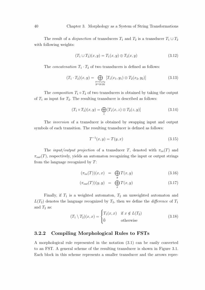
40 Chapter 3. Morphology as a System of String Transformations
The result of a disjunction of transducers T1 and T2 is a transducer T1 ∪ T2
with following weights:
(T1 ∪ T2)(x, y) = T1(x, y)⊕ T2(x, y) (3.12)
The concatenation T1 · T2 of two transducers is defined as follows:
(T1 · T2)(x, y) =⊕
x=x1x2y=y1y2
[T1(x1, y1)⊗ T2(x2, y2)] (3.13)
The composition T1 ◦ T2 of two transducers is obtained by taking the outputof T1 as input for T2. The resulting transducer is described as follows:
(T1 ◦ T2)(x, y) =⊕z
[T1(x, z)⊗ T2(z, y)] (3.14)
The inversion of a transducer is obtained by swapping input and outputsymbols of each transition. The resulting transducer is defined as follows:
T−1(x, y) = T (y, x) (3.15)
The input/output projection of a transducer T , denoted with πin(T ) andπout(T ), respectively, yields an automaton recognizing the input or output stringsfrom the language recognized by T :
(πin(T ))(x, x) =⊕y
T (x, y) (3.16)
(πout(T ))(y, y) =⊕x
T (x, y) (3.17)
Finally, if T1 is a weighted automaton, T2 an unweighted automaton andL(T2) denotes the language recognized by T2, then we define the difference of T1
and T2 as:
(T1 \ T2)(x, x) =
T1(x, x) if x /∈ L(T2)
0 otherwise(3.18)
3.2.2 Compiling Morphological Rules to FSTs
A morphological rule represented in the notation (3.1) can be easily convertedto an FST. A general scheme of the resulting transducer is shown in Figure 3.1.Each block in this scheme represents a smaller transducer and the arrows repre-
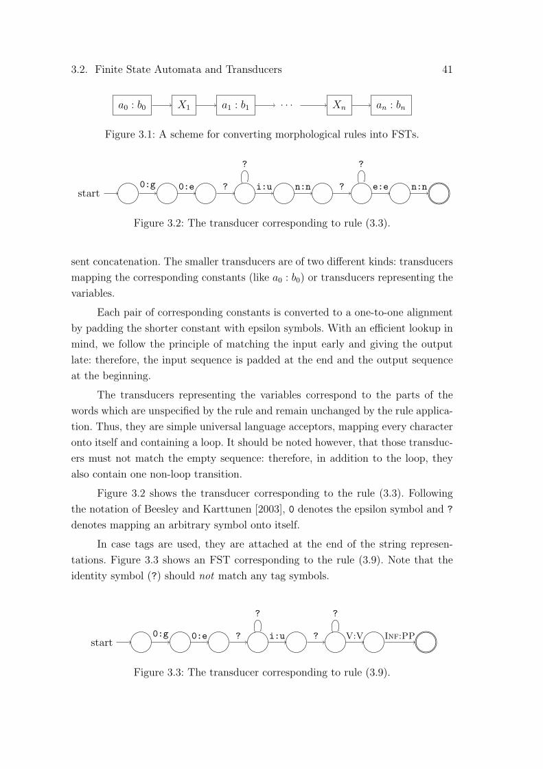
3.2. Finite State Automata and Transducers 41
a0 : b0 X1 a1 : b1 . . . Xn an : bn
Figure 3.1: A scheme for converting morphological rules into FSTs.
start0:g 0:e ?
?
i:u n:n ?
?
e:e n:n
Figure 3.2: The transducer corresponding to rule (3.3).
sent concatenation. The smaller transducers are of two different kinds: transducersmapping the corresponding constants (like a0 : b0) or transducers representing thevariables.
Each pair of corresponding constants is converted to a one-to-one alignmentby padding the shorter constant with epsilon symbols. With an efficient lookup inmind, we follow the principle of matching the input early and giving the outputlate: therefore, the input sequence is padded at the end and the output sequenceat the beginning.
The transducers representing the variables correspond to the parts of thewords which are unspecified by the rule and remain unchanged by the rule applica-tion. Thus, they are simple universal language acceptors, mapping every characteronto itself and containing a loop. It should be noted however, that those transduc-ers must not match the empty sequence: therefore, in addition to the loop, theyalso contain one non-loop transition.
Figure 3.2 shows the transducer corresponding to the rule (3.3). Followingthe notation of Beesley and Karttunen [2003], 0 denotes the epsilon symbol and ?denotes mapping an arbitrary symbol onto itself.
In case tags are used, they are attached at the end of the string represen-tations. Figure 3.3 shows an FST corresponding to the rule (3.9). Note that theidentity symbol (?) should not match any tag symbols.
start0:g 0:e ?
?
i:u ?
?
V:V Inf:PP
Figure 3.3: The transducer corresponding to rule (3.9).
42 Chapter 3. Morphology as a System of String Transformations
3.2.3 Binary Disjunction
In further applications, we will often use a transducer corresponding to the dis-junction of all known morphological rules. While building large transducers usingdisjunction, we have to be careful about when to minimize. On one hand, it isdesirable to operate on minimized transducers as often as possible. On the otherhand, minimization can be a costly operation – especially for large transducersdue to its high theoretical complexity6 – so we should try to keep the number oftimes it has to be called low and the size of the transducers it is called on small.Hence, the following two straightforward strategies for disjuncting a large numberof transducers are both inefficient:
1. Applying all disjunctions first and minimizing the resulting transducer.
2. Disjuncting with one transducer at a time and applying minimization aftereach disjunction.
Instead, I propose a strategy inspired by the well-known algorithm of binaryexponentiation. The idea is to always apply minimization on a disjunction of twominimized transducers of equal size in order to obtain a minimal transducer twicethat size. By ‘size’, I mean the number of elementary transducers (from the inputdata) contained in the given transducer.
Algorithm 3.1 presents the binary disjunction procedure. It utilizes two stacks:S1 for storing intermediary transducers, and S2 for storing their correspondingsizes. Note that the sizes are always powers of two, because a disjunction of twotransducers of equal size yields a transducer twice as large. At each step of theiteration, we check whether the top of the stack contains two transducers of equalsize (we assume that the functions First and Second return the top and next-to-top element without removing it from the stack). If so, we remove them fromthe stack and replace them with their minimized disjunction (lines 6-7). If not, wepush an additional transducer from the input data to the stack with size 1 (lines10-12). In case there are no more transducers left, the loop terminates.
After executing the loop in lines 4-17, S1 contains transducers, the sizes ofwhich are different powers of two (together they make up the binary representationof n). The resulting transducer is a disjunction of all that are left on the stack.This disjunction is computed in lines 19-21. As it typically involves only severaltransducers, it is sufficient to minimize only once after performing all disjunctions.6By minimization, I mean here the operation that yields a minimal deterministic transducer
equivalent to the given one. Determinization is thus implicitly part of minimization. The worst-case complexity of determinization is exponential.

3.2. Finite State Automata and Transducers 43
Algorithm 3.1: Binary disjunction.Input: Transducers T1, T2, . . . , Tn to disjunct.Output: T =
⋃i Ti
1 S1 ← Stack() ;2 S2 ← Stack() ;3 i← 1 ;4 while True do5 if Size(S2) 2 ∧ First(S2) = Second(S2) then6 Push(S1,Minimize(Pop(S1) ∪Pop(S1))) ;7 Push(S2,Pop(S2) +Pop(S2)) ;8 else9 if i ¬ n then10 Push(S1, Ti) ;11 Push(S2, 1) ;12 i← i+ 1 ;13 else14 break ;15 end16 end17 end18 T ← Pop(S1) ;19 while ¬Empty(S1) do20 T ← T ∪Pop(S1) ;21 end22 T ←Minimize(T) ;23 return T

44 Chapter 3. Morphology as a System of String Transformations
100 200 300 400 500 600 700 800 900 1000
0
20
40
Number of transducers
Dis
junc
tion
tim
e(s
ec.)
naive-1 (minimize once)naive-2 (minimize every time)
binary
1000 2000 3000 4000 5000 6000 7000 8000 9000
0
2,000
4,000
Number of transducers
Dis
junc
tion
tim
e(s
ec.)
naive-1 (minimize once)naive-2 (minimize every time)
binary
Figure 3.4: A comparison of running times for different disjunction strategies.

3.2. Finite State Automata and Transducers 45
Figure 3.4 presents computation times of the two naıve strategies and thebinary disjunction for different numbers of transducers. The difference is very clear:for the largest input, which consisted of 8970 transducers (each corresponding toa morphological rule), binary disjunction needed only 31.8 seconds, compared to5080 sec. and 968 sec. for the two naıve strategies.
3.2.4 Computing the Number of Paths in an Acyclic FST
For the purpose of the probabilistic model developed in Sec. 4.1, we will need tobe able to compute the number of distinct paths in an acyclic7 transducer. As thistask is not covered in the standard libraries and extracting all paths in order tocount them is clearly wasteful, we will develop a dynamic programming algorithmfor this purpose.
Let si,q denote the number of distinct paths of length i ending in state q. Thisnumber can be computed using the following recursive formula:
s0,q =
1 if q = q0
0 otherwise(3.19)
s(i+1),q =∑
(q′,a,b,w,q′′)∈Eq′′=q
si,q′ (3.20)
The number of paths of length i+1 ending in state q is thus the number of paths oflength i leading to states, from which q can be reached by one transition, multipliedby the number of transitions leading from such states to q. The number of pathsnpaths can be obtained by summing si,q for all final states:
npaths =∑i
∑q∈F
si,q (3.21)
In practice, we do not need to keep all the values si,q. At each iteration, weonly need the values from the previous iteration. We thus denote the value forstate q from the previous iteration with sq and the value computed at the currentiteration with s′q.
Algorithm 3.2 presents the complete pseudocode. As we do not know themaximum path length, the iteration proceeds until s′q = 0 for every state. Wedenote the set of transitions leaving state q of the transducer T with TrT (q) andthe target state of a transition t with tgt(t).
7This question is not relevant for cyclic transducers, as they have an infinite number of paths.

46 Chapter 3. Morphology as a System of String Transformations
Algorithm 3.2: Computing the number of paths in an acyclic DFST.Input: An acyclic DFST T = (Σ,∆, Q, q0, F, E, ρ).Output: npaths = |PT ({q0}, F )|.npaths ← 0 ;sq0 ← 1 ;changed← true ;sq ← 0 for each q ∈ Q \ {q0} ;while changed dochanged← false ;s′q ← 0 for each q ∈ Q ;for q ∈ Q do
if sq > 0 thenfor t ∈ TrT (q) do
z ← tgt(t) ;s′z ← s′z + sq ;changed← true ;
endend
endfor q ∈ F do
npaths ← npaths + s′q ;endsq ← s′q for each q ∈ Q ;
endreturn npaths

3.2. Finite State Automata and Transducers 47
The time complexity of the algorithm is O(nm), where n is the number ofstates and m is the maximum path length. This holds under the assumption thatthe function Tr(·) operates in constant time, which can be achieved by hashing.The space complexity is O(n), as we store the values sq and s′q for every state.
3.2.5 Learning Probabilistic Automata
Probabilistic automata, i.e. weighted automata over the probability semiring, de-fine probability distributions over regular languages. The learning of such automatais a statistical inference problem, in which the automaton is reconstructed from asample from its distribution. This section presents one particular algorithm suitedfor this task, called ALERGIA [de la Higuera and Thollard 2000; de la Higuera2010].
ALERGIA is a representative of the group of state-merging algorithms : itbegins by constructing an automaton exactly reflecting the sample distribution, theso-called prefix tree acceptor. Then, pairs of similar states are identified and merged,which results in a generalization of the distribution. In order to identify whether thestates can be merged, the so-called ALERGIA test (Algorithm 3.5) is used, whichchecks whether the differences in transition probabilities are statistically significant.Provided that the sample is indeed generated from a probabilistic automaton,ALERGIA is proven to identify the ‘true’ automaton in the limit (i.e. for arbitrarilylarge sample sizes) with probability one [de la Higuera and Thollard 2000].
The following presentation of the ALERGIA algorithm is based on de laHiguera [2010]. We will start by defining a frequency automaton, which can beused to reflect a multiset of strings:
Definition 3.8. A deterministic frequency finite automaton (DFFA) is a tupleA = (Σ, Q, Ifr,Ffr, δfr) where Σ is the alphabet, Q is a finite set of states, Ifr :Q 7→ N is the initial state frequency function, Ffr : Q 7→ N is the final statefrequency function, and δfr : Q×Σ×Q 7→ N is the transition frequency function.
A frequency automaton is similar to a weighted automaton in that eachtransition and final state is labeled with a weight, in this case a natural numberrepresenting frequency. The following property requires that the sum of frequenciesentering a state equals the sum of frequencies leaving it, which is necessary if theweights are supposed to reflect frequency:
Definition 3.9. A DFFA A = (Σ, Q, Ifr,Ffr, δfr) is said to be well defined if∀q ∈ Q : Ifr(q) +
∑q′∈Qa∈Σ
δfr(q′, a, q) = Ffr(q) +∑q′∈Qa∈Σ
δfr(q, a, q′).

48 Chapter 3. Morphology as a System of String Transformations
A DFFA can be easily converted into a probabilistic automaton by dividingthe frequency of each transition or final state by the sum of frequencies leaving thestate (including its final frequency). The latter value will be called state frequencyand written as FREQ(q).
The sample, from which the distribution will be learned, will be representedby a special kind of automaton, called frequency prefix tree acceptor, which isdefined as follows:
Definition 3.10. Let S be a multiset of strings from Σ∗ and Pref(S) denote theset of prefixes of strings from S. The frequency prefix tree acceptor FPTA(S) is theDFFA (Σ, Q, Ifr,Ffr, δfr) where:
• Q = {qu : u ∈ Pref(S)},
• Ifr(qε) = |S|,
• ∀ua ∈ Pref(S), δfr(qu, a, qua) = |S|uaΣ∗ ,
• ∀u ∈ Pref(S),Ffr(qu) = |S|u.
The key element of a state-merging algorithm is merging a pair of stateswhich are deemed to be indistinguishable. This is realized by the STOCHASTIC-MERGE operation (Algorithm 3.3). The state q′ is merged into q by transferringthe incoming transition, together with its frequency, to q. Then, the subtree rootedin q′ has to be merged with the one rooted in q. This is realized by the recursiveoperation STOCHASTIC-FOLD (Algorithm 3.4).
Algorithm 3.3: STOCHASTIC-MERGE.Input: a DFFA A, 2 states q, q′ to be mergedOutput: A updated, with q and q′ mergedLet (qf , a) be such that δA(qf , a) = q′;n← δfr(qf , a, q′);δA(qf , a)← q;δfr(qf , a, q)← n;δfr(qf , a, q′)← 0;return STOCHASTIC-FOLD(A, q, q′)
We use the algorithm ALERGIA-COMPATIBLE (Algorithm 3.6) to deter-mine whether two states can be merged. The algorithm calls ALERGIA-TEST(Algorithm 3.5) on the final frequencies of the states and on the frequencies of

3.2. Finite State Automata and Transducers 49
Algorithm 3.4: STOCHASTIC-FOLD.Input: a DFFA A, 2 states q and q′
Output: A updated, where subtree in q′ is folded into qFfr(q)← Ffr(q) + Ffr(q′);for a ∈ Σ such that δA(q′, a) is defined do
if δA(q, a) is defined thenδfr(q, a, δA(q, a))← δfr(q, a, δA(q, a)) + δfr(q′, a, δA(q′, a));A ← STOCHASTIC-FOLD(A, δA(q, a), δA(q′, a));
elseδA(q, a)← δA(q′, a);δfr(q, a, δA(q, a))← δfr(q′, a, δA(q′, a))
endendreturn A
each outgoing transition. The test states whether the difference between frequen-cies is statistically insignificant. The theoretical foundation for the formula is theHoeffding bound [de la Higuera 2010, p. 199]: if the frequencies f1, f2 are generatedfrom the same Binomial distribution, the test is passed with probability at least(1−α)2. Two states can be merged if the test is passed for all frequencies. Smallervalues of α mean laxer bounds on the difference between frequencies generatedfrom the same distribution, and thus easier merging.
Algorithm 3.5: ALERGIA-TEST.Input: f1, n1, f2, n2, α > 0Output: a Boolean indicating whether f1
n1and f2
n2are sufficiently close
γ ←∣∣∣ f1n1− f2
n2
∣∣∣;return
[γ <
(√1n1
+√
1n2
)·√
12 ln 2
α
]
We can now turn to the description of the ALERGIA algorithm (Algorithm3.7). Given a sample S of strings, it starts by building a prefix tree acceptor forthis sample. Subsequently, certain states are marked as Red or Blue. The Redstates are the ones which are certainly going to be part of the resulting automaton.The Blue states are candidates for merging with a Red state. Initially, the setof Red states consists only of the initial state, corresponding to the empty prefix,while the set of Blue states consists of all the children of the initial state.
The algorithm proceeds by iteratively choosing a Blue state qb and attempt-ing to merge it with one of the Red states. If no merge is possible, qb is ‘promoted’,i.e. it becomes itself a Red state. At the end of each iteration, the set of Blue

50 Chapter 3. Morphology as a System of String Transformations
Algorithm 3.6: ALERGIA-COMPATIBLE.Input: an FFA A, two states qu, qv, α > 0Output: qu and qv compatible?Correct← true;if ¬ALERGIA-TEST(FPA(qu),FREQA(qu),FPA(qv),FREQA(qv), α) then
Correct← false;endfor a ∈ Σ do
if ¬ALERGIA-TEST(δfr(qu, a),FREQA(qu), δfr(qv, a),FREQA(qv), α)then
Correct← false;end
endreturn Correct
states is updated to include all children of Red states, which are not Red statesthemselves. The loop terminates if there are no Blue states left.
The parameter t0 denotes the minimum frequency of a state to be consideredfor merging. For states with low frequency, we assume to have too little informationto make any statistically informed decision on whether to merge them. In order toavoid overgeneralization, we leave such states out.
Algorithm 3.7: ALERGIA.Input: a sample S, α > 0, t0Output: an FFA AA ← FPTA(S) ;Red← {qε} ;Blue← {qa : a ∈ Σ ∩Pref(S)} ;while CHOOSE qb from Blue such that FREQ(qb) t0 do
if ∃qr ∈ Red : ALERGIA-COMPATIBLE(A, qr, qb, α) thenA ← STOCHASTIC-MERGE(A, qr, qb)
elseRed← Red ∪ {qb}
endBlue← {qua : ua ∈ Pref(S) ∧ qu ∈ Red} \Red
endreturn A

3.3. Rule Extraction 51
3.3 Rule Extraction
The first step to learning systematic structural correspondences between words isthe extraction of candidate patterns from pairs of words which are likely to bemorphologically related, i.e. sufficiently similar in terms of string edit distance.This task will be achieved in two stages: finding pairs of similar words (Sec. 3.3.1)and extraction of rules from word pairs (Sec. 3.3.2). The result of those two stepscombined is a directed graph, in which words are vertices and the postulated mor-phological relations edges. A filtering of the graph according to some simple criteria(Sec. 3.3.3) removes a lot of noise and greatly diminishes the density of the graph.Placing further restrictions on admissible graph edges can introduce a certain de-gree of supervision, up to fully supervised training (Sec. 3.3.4).
3.3.1 Finding Pairs of Similar Words
For the task of finding pairs of similar words, we employ a slightly modified versionof the FastSS algorithm [Bocek et al. 2007]. In its original version, the algorithmfinds all pairs of words with Levenshtein distance8 at most k in a given wordlist. It works by creating a deletion neighborhood for each word, consisting of allsubstrings obtainable by performing up to k deletions on the given word. The wordsare subsequently grouped according to the substrings (e.g. by sorting or hashing).Finally, the Levenshtein distance is computed for each pair of words sharing asubstring. For small k (¬ 3), the algorithm has been shown to outperform severalalternative approaches, like Neighborhood Generation or n-gram cosine similarity,among others.
For the purpose of discovering potential morphological rules, it is reasonableto modify the notion of edit distance. Firstly, morphological rules usually oper-ate on groups of consecutive letters, rather than single letters independently, sodeletion or substitution of a segment of consecutive letters should yield higher sim-ilarity than deletion or substitution of the same number of non-consecutive letters.Secondly, although we are going to permit word-internal alternations, more changeshould be permitted at the beginning and at the end of words, since that is wheremost morphological rules operate. Bearing in mind the representation (3.1), let laffix
denote the maximum length of a morphological constant at the beginning or the
8The Levenshtein distance, a.k.a. string edit distance [Levenshtein 1966; Wagner and Fischer1974] between two strings is the minimum number of elementary edit operations, i.e. deletions,insertions or substitutions of a single symbol, needed to transform one of the strings into theother.

52 Chapter 3. Morphology as a System of String Transformations
0start 1 2 3 4 5
6789
10 11 12 13 14 15
?:δ ?:δ ?:δ ?:δ ?:δ
0
0
0
0
0
?
?
?:δ?:δ?:δ
0
0
0?
?
?:δ ?:δ ?:δ ?:δ ?:δ
0
0
0
0
0
Figure 3.5: The transducer S1 for generating a deletion neighborhood.
end of a word (a0, b0, an, bn in (3.1)), linfix the maximum length of a morphologicalconstant inside the word (ai, bi for 0 < i < n in (3.1)) and kmax the maximumnumber of variables. In order to generate pairs which are related by a rule satisfy-ing this constraint, we obtain the following constraints on a deletion environment:deleting up to laffix consecutive letters at the beginning and end of the word, andup to linfix consecutive letters in at most kmax − 1 slots inside the word. The usualsetting for those parameters, which covers a vast majority of morphological rulesencountered in practice, is laffix = 5, linfix = 3, kmax = 2.
Such settings allow for deletion of up to 13 letters in total, so that even formiddle-length words it would consider all pairs to be similar. In order to preventthis, we introduce an additional constraint: the total amount of deleted charactersmust be smaller than half of the word’s length. In this way, we can consider longaffixes, but only if enough of the word is still left to form a recognizable stem.
With all those constraints, computing a deletion neighborhood of a word becomesa complex operation. It is therefore helpful to visualize and implement it usingtransducers. We will construct the transducer S mapping words to their deletion
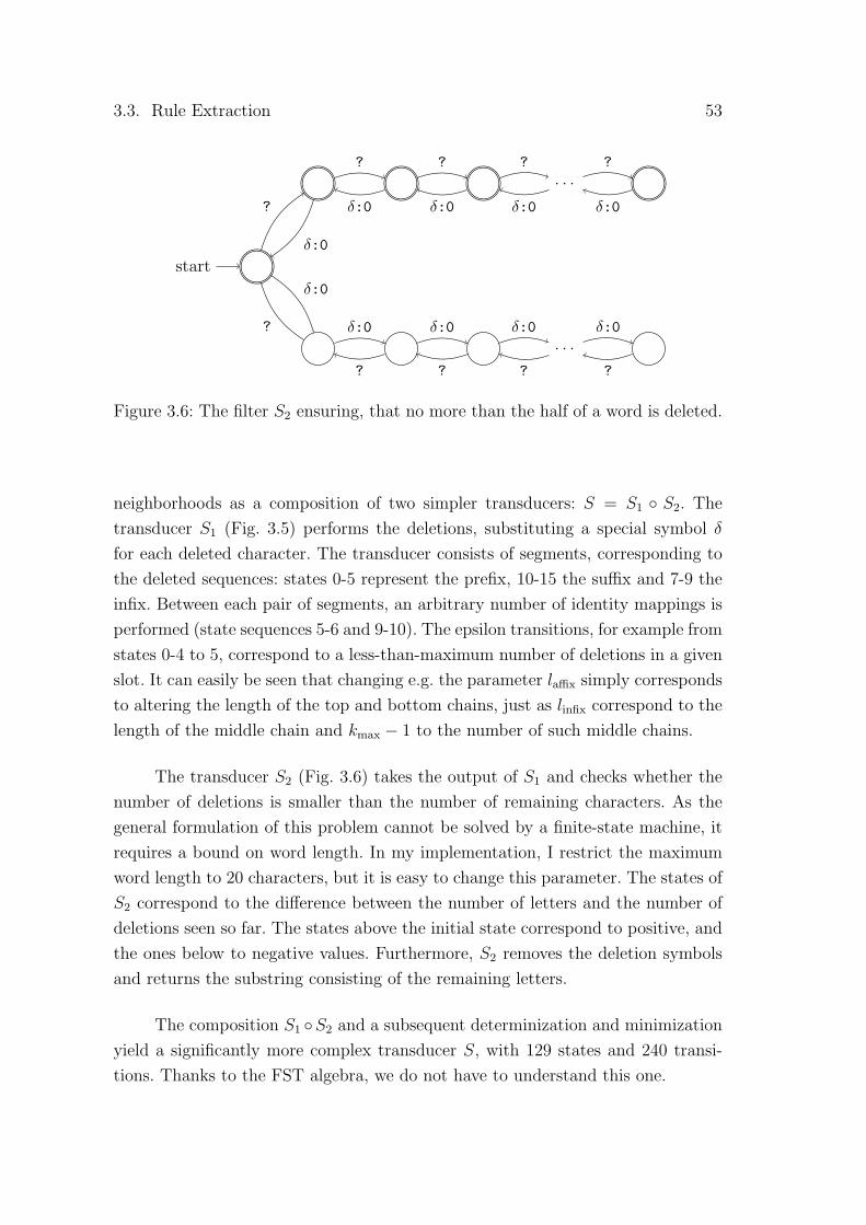
3.3. Rule Extraction 53
start
. . .
. . .
????
?
?
? ? ? ?
δ:0δ:0δ:0δ:0
δ:0
δ:0
δ:0 δ:0 δ:0 δ:0
Figure 3.6: The filter S2 ensuring, that no more than the half of a word is deleted.
neighborhoods as a composition of two simpler transducers: S = S1 ◦ S2. Thetransducer S1 (Fig. 3.5) performs the deletions, substituting a special symbol δfor each deleted character. The transducer consists of segments, corresponding tothe deleted sequences: states 0-5 represent the prefix, 10-15 the suffix and 7-9 theinfix. Between each pair of segments, an arbitrary number of identity mappings isperformed (state sequences 5-6 and 9-10). The epsilon transitions, for example fromstates 0-4 to 5, correspond to a less-than-maximum number of deletions in a givenslot. It can easily be seen that changing e.g. the parameter laffix simply correspondsto altering the length of the top and bottom chains, just as linfix correspond to thelength of the middle chain and kmax − 1 to the number of such middle chains.
The transducer S2 (Fig. 3.6) takes the output of S1 and checks whether thenumber of deletions is smaller than the number of remaining characters. As thegeneral formulation of this problem cannot be solved by a finite-state machine, itrequires a bound on word length. In my implementation, I restrict the maximumword length to 20 characters, but it is easy to change this parameter. The states ofS2 correspond to the difference between the number of letters and the number ofdeletions seen so far. The states above the initial state correspond to positive, andthe ones below to negative values. Furthermore, S2 removes the deletion symbolsand returns the substring consisting of the remaining letters.
The composition S1 ◦S2 and a subsequent determinization and minimizationyield a significantly more complex transducer S, with 129 states and 240 transi-tions. Thanks to the FST algebra, we do not have to understand this one.

54 Chapter 3. Morphology as a System of String Transformations
We can now generate all pairs of similar words from a lexicon automaton L byperforming the following composition:
P = (L ◦ S) ◦ (L ◦ S)−1 (3.22)
There are various ways to implement this in practice. Computing the compositiondirectly is usually not feasible because of high memory complexity. One possibilityis to use S for substring generation, but otherwise proceed as in the original FastSSalgorithm: store the words and substrings in an index structure, either on disk orin memory, then retrieve words for each substring. Another possibility is to useS to generate substrings for a given word and then look the substrings up inthe transducer (L ◦ S)−1 to obtain similar words. The latter composition can becomputed statically. While the second approach is significantly slower, it has anadvantage in providing a way to retrieve all words w′ similar to a given word w atonce. It is thus better suited for parallelization, especially in case the pairs (w,w′)are subject to further processing.
3.3.2 Extraction of Rules from Word Pairs
Given a pair (w,w′) of string-similar words, we want to extract morphological rulesmodeling the difference between those words. For this purpose, we first align thewords on character-to-character basis and then attribute each character mappingeither to a morphological constant or a variable.
Algorithm 3.8 is used to compute the optimal alignment between two words.It is a variant of the well-known dynamic programming algorithm for computingedit distance [Wagner and Fischer 1974]. In addition to the distance matrix D,three further matrices are used. Ξ remembers the last edit operation at each point.It can be used to reconstruct the optimal alignment after having computed the editdistance. Beginning in the bottom right corner, the arrows in Ξ show the optimalpath. The matrices X and Y contain the character that is consumed respectivelyfrom word w or w′ by the current edit operation.
After building the matrices D,Ξ, X, Y , the function Extract-alignment(Algorithm 3.9) walks the path from the bottom right to the top left corner byfollowing the arrows in matrix Ξ. At each step, a pair of characters from thecorresponding cells in matrices X and Y is picked as an element of the alignment.
The workings of Algorithm 3.8 are illustrated in Figure 3.7. In an actualimplementation, there is no need to store the matrices Ξ, X, Y explicitly, as the

3.3. Rule Extraction 55
Algorithm 3.8: Aligning similar words with minimum number of editoperations.
Input: w,w′ – string-similar wordsOutput: u, v – sequences of characters representing the optimal alignmentd0,0 ← 0 ; x0,0 ← ε ; y0,0 ← ε ; ξ0,0 ← ‘?’ ;for i← 1 to |w|+ 1 do
d0,i ← d0,(i−1) + 1 ; xj,i ← wi ; yj,i ← ε ; ξj,i ← ‘← ’ ;endfor j ← 1 to |w′|+ 1 do
dj,0 ← d(j−1),0 + 1 ; xj,i ← ε ; yj,i ← w′j ; ξj,i ← ‘ ↑ ’ ;for i← 1 to |w|+ 1 do
dj,i ← min[d(j−1),i + 1, dj,(i−1) + 1, d(j−1),(i−1) + δ(wi, w′j)
];
if dj,i = d(j−1),(i−1) + δ(wi, w′j) thenxj,i ← wi ; yj,i ← w′j ; ξj,i ← ‘↖ ’ ;
else if dj,i = dj,(i−1) + 1 thenxj,i ← wi ; yj,i ← ε ; ξj,i ← ‘← ’ ;
elsexj,i ← ε ; yj,i ← w′j ; ξj,i ← ‘ ↑ ’ ;
endend
endu, v ← Extract-alignment(X, Y,Ξ, |w|, |w′|) ;return u, v
Algorithm 3.9: Extract-alignment.Input: X, Y,Ξ, n,mOutput: u, v – alignmenti← n ; j ← m ; k ← 0 ;while i > 0 or j > 0 do
uk ← xj,i ; vk ← yj,i ; k ← k + 1 ; i′ ← i ;if ξj,i ∈ {↖,←} then
i← i− 1 ;endif ξj,i′ ∈ {↖, ↑} then
j ← j − 1 ;end
endreturn reverse(u),reverse(v)
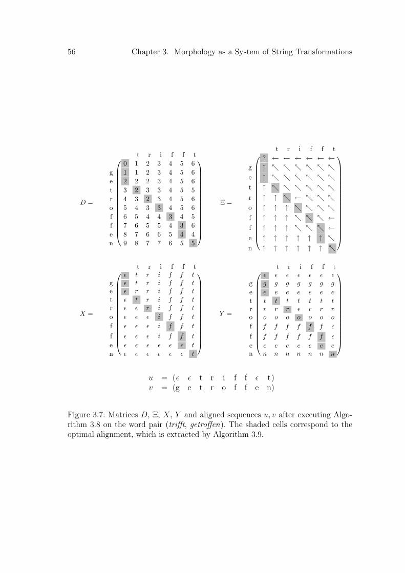
56 Chapter 3. Morphology as a System of String Transformations
D =
t r i f f t
0 1 2 3 4 5 6g 1 1 2 3 4 5 6e 2 2 2 3 4 5 6t 3 2 3 3 4 5 5r 4 3 2 3 4 5 6o 5 4 3 3 4 5 6f 6 5 4 4 3 4 5f 7 6 5 5 4 3 6e 8 7 6 6 5 4 4n 9 8 7 7 6 5 5
Ξ =
t r i f f t
? ← ← ← ← ← ←g ↑ ↖ ↖ ↖ ↖ ↖ ↖e ↑ ↖ ↖ ↖ ↖ ↖ ↖t ↑ ↖ ↖ ↖ ↖ ↖ ↖r ↑ ↑ ↖ ← ↖ ↖ ↖o ↑ ↑ ↑ ↖ ↖ ↖ ↖f ↑ ↑ ↑ ↖ ↖ ↖ ←f ↑ ↑ ↑ ↖ ↖ ↖ ←e ↑ ↑ ↑ ↑ ↑ ↑ ↖n ↑ ↑ ↑ ↑ ↑ ↑ ↖
X =
t r i f f t
ε t r i f f tg ε t r i f f te ε r r i f f t
t ε t r i f f tr ε ε r i f f t
o ε ε ε i f f t
f ε ε ε i f f t
f ε ε ε i f f t
e ε ε ε ε ε ε t
n ε ε ε ε ε ε t
Y =
t r i f f t
ε ε ε ε ε ε εg g g g g g g g
e e e e e e e e
t t t t t t t tr r r r ε r r ro o o o o o o o
f f f f f f f ε
f f f f f f f ε
e e e e e e e en n n n n n n n
( )u = ε ε t r i f f ε t( )v = g e t r o f f e n
Figure 3.7: Matrices D, Ξ, X, Y and aligned sequences u, v after executing Algo-rithm 3.8 on the word pair (trifft, getroffen). The shaded cells correspond to theoptimal alignment, which is extracted by Algorithm 3.9.

3.3. Rule Extraction 57
values on the optimal path can be easily reconstructed while walking through D.However, they are shown here for the purpose of presentation and simplifying thepseudocode.
Given the alignment, we construct rules by turning sequences of identity map-pings into variables. As identity mappings may also be parts of constants (describ-ing the context in which a rule applies), many different rules can be extractedfrom a single pair. In order to compute them, we will use an auxiliary object calledmask. A mask is a sequence of dashes and asterisks, like --**-**--. Applied to analignment, it expresses that mappings at a position marked with a dash are partsof a constant, while mappings at a position marked with an asterisk are parts ofa variable. Thus, applied to the mapping (u, v) from Figure 3.7, the above maskyields the rule /X1iX2t/→ /geX1oX2en/.
Algorithm 3.10 extracts the rules from a pair of words using the alignmentalgorithm described above. As converting a mask to a rule, realized by the func-tion Make-Rule-From-Mask, is straightforward, the description of this step isskipped. Thus, the algorithm describes computing the different masks from a givenalignment. The parameters kmax, laffix, linfix are used with the same meaning as inprevious section.
The masks are computed incrementally on prefixes of the alignment. A pri-ority queue is used to store the unfinished masks. Each queue item is a sextuple〈s, i, k, lx, ly, z〉, with s being the current mask prefix, i the position in the alignmentto be considered next, k the current number of variables (consecutive sequences ofasterisks), lx and ly the lengths of the currently constructed constants (respectivelyon the left and right side) and z a Boolean variable stating, whether the currentlyconstructed constant is a suffix (i.e. if z = True, no more asterisks are allowed).
Initially, the queue contains one item, corresponding to an empty mask (line3). In each iteration, one element is taken from the queue and considered. If i > |u|,the whole alignment has been processed and s contains a complete mask. In thiscase, the resulting rule is added to the result set (line 7). Otherwise, the nextcharacter pair in the alignment (ui, vi) is considered and either a dash or an asteriskis appended to the mask. As there might be multiple possible results of this step,each possibility is added to the queue for further processing. The various cases arisefrom the requirement on the mask to comply with the restrictions kmax, laffix, linfix.
First, let us consider the case where ui = vi (lines 9-27). The pair (ui, vi)can then be added either to a constant or to a variable. The first two subcasesconsider appending the pair to either a prefix (lines 10-12) or a suffix (lines 13-15).

58 Chapter 3. Morphology as a System of String Transformations
Algorithm 3.10: Extracting rule candidates from pairs of similar words.Input: w,w′ – string-similar words; kmax – max. number of variables;
linfix, laffix – max. length of infixes/affixes.Output: R – a set of rules extracted from (w,w′)
1 u, v ← Align(w,w′);2 q ← Queue(); R← ∅;3 Enqueue(q, 〈ε, 1, 0, 0, 0,False〉);4 while not Empty(q) do5 〈s, i, k, lx, ly, z〉 ← Dequeue(q);6 if i > |u| then7 R← R ∪ {Make-Rule-From-Mask(u, v, s)};8 else9 if ui = vi then10 if k = 0 ∧max{lx, ly} < laffix then11 Enqueue(q, 〈s · ‘-’, i+ 1, k, lx + 1, ly + 1, z〉);12 end13 if k > 0 ∧max{lx, ly} < laffix then14 Enqueue(q, 〈s · ‘-’, i+ 1, k, lx + 1, ly + 1,True〉);15 end16 if not z then17 if k > 0 ∧max{lx, ly} < linfix then18 Enqueue(q, 〈s · ‘-’, i+ 1, k, lx + 1, ly + 1, z〉);19 end20 if si−1 6= ‘*’ then21 if k < kmax then22 Enqueue(q, 〈s · ‘*’, i+ 1, k + 1, 0, 0, z〉);23 end24 else25 Enqueue(q, 〈s · ‘*’, i+ 1, k, 0, 0, z〉);26 end27 end28 else29 if (k = 0 ∧max{lx, ly} < laffix) ∨max{lx, ly} < linfix then30 Enqueue(q, 〈s · ‘-’, i+ 1, k, lx + 1− δ(ui, ε), ly + 1− δ(vi, ε), z〉);31 else if max{lx, ly} < laffix then32 Enqueue(q, 〈s · ‘-’, i+ 1, k, lx + 1− δ(ui, ε), ly + 1−
δ(vi, ε),True〉);33 end34 end35 end36 return R

3.3. Rule Extraction 59
u ε ε t r i f f ε tv g e t r o f f e n
/X1iX2t/→ /geX1oX2en/ – – * * – * * – –/X1ifX2t/→ /geX1ofX2en/ – – * * – – * – –/X1iX2ft/→ /geX1oX2fen/ – – * * – * – – –/X1riX2t/→ /geX1roX2en/ – – * – – * * – –/tX1iX2t/→ /getX1oX2en/ – – – * – * * – –/tX1iX2ft/→ /getX1oX2fen/ – – – * – * – – –/X1riX2ft/→ /geX1roX2fen/ – – * – – * – – –/X1rifX2t/→ /geX1rofX2en/ – – * – – – * – –
/Xifft/→ /geXoffen/ – – * * – – – – –/triXt/→ /getroXen/ – – – – – * * – –
/tX1ifX2t/→ /getX1ofX2en/ – – – * – – * – –/triXft/→ /getroXfen/ – – – – – * – – –/tXifft/→ /getXoffen/ – – – * – – – – –
Figure 3.8: Rules extracted from the pair (trifft, getroffen) by Algorithm 3.10 andtheir corresponding masks, sorted by generality.
Furthermore, it can also be added to an infix (lines 17-19) or to a variable (lines20-27). The latter two subcases are only possible if z is false, as an infix mustbe followed by a variable (otherwise it would be a suffix) and the last subcaseitself extends a variable, i.e. adds an asterisk to the mask. In the last subcase, wealso distinguish whether the variable has to be newly created (lines 21-23), or analready existing variable is extended (lines 24-26).
The second major case is ui 6= vi (lines 28-34). Then, the pair (ui, vi) can onlybe added to a constant. The two subcases ensure that the currently constructedconstant does not exceed the maximum length. The first subcase (lines 29-30)accounts for a prefix or an infix and the second (lines 31-32) for a suffix.
In lines 30 and 32, δ(·, ·) denotes the Kronecker delta, which is 1 if botharguments are equal and 0 otherwise. This is due to the fact that adding an epsilonto a constant does not increase its length (as nothing is added). Those terms canbe skipped in the case ui = vi, because the alignment must not contain pairs (ε, ε).
As the case ui = vi has two possible outcomes (adding either a dash or anasterisk), concern may arise whether the algorithm has exponential complexity.However, the limitation of at most kmax sequences of consecutive asterisks and atmost linfix consecutive dashes between asterisks greatly constrain the number ofpossibilities, especially as those parameters are typically set to very small values(kmax = 2, linfix = 3). With such settings, no runtime problems arise.
Figure 3.8 illustrates the results of Algorithm 3.10 for the pair (trifft, getrof-

60 Chapter 3. Morphology as a System of String Transformations
rank rule frequency example
1 /Xn/→ /X/ 8555 Epoche → Epochen2 /X/→ /Xn/ 8555 Epochen → Epoche3 /Xen/→ /Xe/ 7465 aufgehenden → aufgehende4 /Xe/→ /Xen/ 7465 aufgehende → aufgehenden5 /Xen/→ /X/ 6030 Abkurzungen → Abkurzung6 /X/→ /Xen/ 6030 Abkurzung → Abkurzungen7 /Xe/→ /X/ 5640 niedrige → niedrig8 /X/→ /Xe/ 5640 niedrig → niedrige9 /Xs/→ /X/ 4917 Erdbebens → Erdbeben
10 /X/→ /Xs/ 4917 Erdbeben → Erdbebens. . .
53 /Xen/→ /Xt/ 1194 nutzen → nutzt54 /Xen/→ /Xes/ 1194 einfachen → einfaches
. . .746 /X1aX2/→ /X1oX2/ 196 unterbrachen → unterbrochen747 /X1tX2/→ /X1mX2/ 195 warten → warmen748 /X1nX2/→ /X1lX2/ 195 Zahnen → Zahlen749 /X1mX2/→ /X1tX2/ 195 warmen → warten750 /X1lX2/→ /X1nX2/ 195 Zahlen → Zahnen751 /X1geX2t/→ /X1X2en/ 195 zugefugt → zufugen752 /{CAP}X1X2/→ /X1schX2/ 195 Allergie → allergische753 /X1schX2/→ /{CAP}X1X2/ 195 allergische → Allergie754 /X1aX2er/→ /X1aX2/ 195 Hauser → Haus755 /X1aX2/→ /X1aX2er/ 195 Haus → Hauser756 /gX/→ /ausgX/ 194 gegraben → ausgegraben757 /ausgX/→ /gX/ 194 ausgegraben → gegraben
Table 3.2: Example rules extracted from the German Wikipedia.
fen). The parameter values are set to laffix = 5, linfix = 3, kmax = 2. All rulessatisfying those requirements are extracted. The rules describe the transformationwithin the word pair with various degrees of generality: the more asterisks a maskcontains, the more general is the resulting rule.
Table 3.2 shows example rules extracted from a corpus of 1 million sentencesfrom German Wikipedia, where only word types with frequency of at least 8 wereconsidered. It can be seen in the bottom of the table that patterns consisting ofa single letter substitution and corresponding to accidental word similarity canbe fairly frequent and get mixed with correct and important morphological rules,like the one deriving Hauser from Haus. For this reason, frequency alone is not agood criterion for determining whether a pattern is truly morphological. This is themotivation for the probabilistic model that will be presented in the next chapter.

3.3. Rule Extraction 61
3.3.3 Filtering the Graph
The graph extracted by the above two steps contains a lot of noise. Infrequentpatterns either correspond to accidental string similarity, or are very specific, likethe last rule in Fig. 3.8. For learning morphology however, only highly regular,general and frequent patterns are of interest. In order to filter out most of thenoise, the criteria listed below are applied.
Minimum rule frequency. In order to be considered candidate for a morpho-logical rule, a pattern has to be supported by a sufficient number of examples.Especially patterns occurring only once are poor candidates. In my experiments, Iusually set this threshold to a value between 3 and 10.
Maximum number of rules. In many practical cases, capturing all rules is notreally important. The number of rules (or, equivalently, edges) may however affectthe runtime and resource usage of statistical inference algorithms used in furtherprocessing. For this reason, it is beneficial to keep the number of rules bounded.The rules are selected according to frequency: restricting the maximum numberto n results in keeping only the n most frequent rules. This parameter is usuallyset to 10, 000, which results in acceptable processing times, while the likelihood ofmissing an important morphological rule is still very low. However, the plausiblevalue might depend on the size of the training data.
Maximum number of edges per word pair. As Figure 3.8 illustrates, oneword pair can yield many rules, most of them being too specific and thus useless. Incase the overspecific rules are frequent, they may survive the two previous filteringsteps and even have harmful effects on further processing, by taking irrelevantdetails into account. In order to prevent that, we allow only the top-n rules foreach word pair, ordered by frequency. This parameter is usually set to between3 and 5. For supervised learning, slightly higher values may be appropriate inorder to capture irregularities and exceptions. On the other hand, higher valuesfor unsupervised learning result in harmful random overfitting.
3.3.4 Supervised and Restricted Variants
Supervised training. The approach for extracting candidate edges describedso far can be easily modified for the task of supervised learning. In this variant,instead of a plain list of words, we obtain a list of word pairs (w,w′), where w′ is

62 Chapter 3. Morphology as a System of String Transformations
supposed to be derived from w. We then simply skip the FastSS step and applyAlgorithm 3.10 directly to the pairs provided by the training data. The result is alist of triples (w,w′, r), with (w,w′) belonging to the training data and r being arule.
Left and right restrictions. The supervised training approach described aboveis equivalent to placing a restriction on admissible edges. Only edges (w,w′, r), forwhich (w,w′) belong to the training data, are allowed.
A similar, but more lax restriction can also be formulated: let VL denote theset of words which are allowed on the left side of rules, and VR the set of wordswhich are allowed on the right side. Then, we can filter the extracted edges byallowing only edges (w,w′, r) satisfying: w ∈ VL ∧ w′ ∈ VR. A canonical examplefor this variant is learning lemmatization from an unlemmatized corpus, when anadditional list of lemmas is provided, as it is done in Sec. 5.3. In this case, VL is thelist of lemmas and VR are the word forms from the corpus that are not containedin VL.
Chapter 4
Statistical Modeling and Inference
The purpose of this chapter is to define a generative probabilistic model of vo-cabularies (sets of words) together with their morphological analysis, much like itis done by Morfessor [Creutz and Lagus 2005a]. However, instead of segmentingwords, the morphological relationships will be expressed as an application of awhole-word rule. In consequence, the morphological analysis takes the form of adirected graph – more specifically, a branching, i.e. a directed forest. The modelis inspired by the Minimum Description Length1 principle: high probability is at-tributed to analyses that make use of morphological rules to eliminate redundanciesamong related words.
In Sec. 4.1 I provide a high-level description of the model. For some of itscomponents, multiple functions are possible – proposals for them are described inSec. 4.2. Finally, in Sec. 4.3, I describe inference methods used to fit the modelparameters to the data.
4.1 Model Formulation
Our present aim is to introduce a probabilistic model defining a probability dis-tribution over graphs such as the one depicted in Figure 4.1, which describe thederivation relation between words. The vertices of the graph are words, while theedges are triplets consisting of a source word, a target word and a rule. The modelthus defines a joint probability of vertices and edges.
The graph illustrates a view on the structure of the lexicon, in which only
1However, the use of continuous parameter spaces makes it difficult to apply MDL directly,so the actual inference is based on the somewhat related methods of Maximum Likelihood andMaximum A-Posteriori likelihood.
63

64 Chapter 4. Statistical Modeling and Inference
relation related relate
relates
relations
relational
correlation
relatedness
/Xtion/→ /Xted/ /Xed/→ /Xe/
/Xed/→ /Xes/
/X/→ /Xs/
/X/→ /Xal/
/X/→/corX/
/X/→ /Xness/
Figure 4.1: An example tree of word derivations.
the root words are listed explicitly. The edges correspond to the information thata rule applies to a certain word. From an information-theoretic perspective, thisresults in a compression of information compared to the case where each word hadto be listed explicitly and independently. The redundancy arising from structuralsimilarities between related words is thus avoided.
4.1.1 The Basic Model
Let V denote the set of vertices of the graph, R the set of known morphologicalrules, E ⊂ V × V × R the set of labeled edges and V0 ⊆ V the set of root nodes.Furthermore, let θ = 〈θroot, θedge〉 denote parameters of the model components,which will be explained in Sec. 4.2. The joint probability of vertices and edgesgiven rules and model parameters is defined as follows:
P (V,E|R,θ) ∝∏v∈V0
λV Proot(v|θroot)
×∏v∈V
∏r∈R
∏v′∈r(v)
pedge(v, v′, r|θedge) if (v, v′, r) ∈ E
1− pedge(v, v′, r|θedge) if (v, v′, r) /∈ E
(4.1)
The model consists of two components: a root distribution Proot and an edgeprobability function pedge. The root distribution is a probability distribution overstrings, defined over whole of Σ+. It is used to generate the root words in thegraph. Each word in the graph generates a set of possible edges, which may ariseby applying a known rule to the word in consideration to derive a new word.The edge probability function pedge assigns a probability to a possible edge. Notethat pedge is not itself a probability distribution: it does not sum to one over all

4.1. Model Formulation 65
possible edges. Rather, for each possible edge (v, v′, r), pedge generates a Bernoullidistribution with success probability pedge(v, v′, r|θedge). λV is a hyperparametercorresponding to the expected number of root nodes. Its inclusion is explained inSec. 4.1.2.
4.1.2 Distributions on Subsets of a Set
Let A be a countable set and f : A 7→ [0, 1] be a probability distribution functionon A. Then we can define a probability distribution g on finite subsets of A in thefollowing way:
g(A) ∝ P (S = |A|) · |A|! ·∏a∈A
f(a) (4.2)
The model consists of drawing a size S of the set and then drawing S elementsaccording to f . The factorial term is due to the fact that the elements can be chosenin any order. Note that the right side of (4.2) does not sum to one over all finitesubsets, because the set elements are drawn with replacement, but multisets arenot included in the domain. However, for our purposes it is sufficient to know thedistribution up to a normalizing constant.
If we assume that the set size S has Poisson distribution, the formula furtherreduces to:
g(A) ∝ e−λλ|A|
|A|!· |A|! ·
∏a∈A
f(a) ∝∏a∈A
λf(a) (4.3)
with λ being the expected set size. In this formulation, we can also view λ as anarbitrarily defined marginal cost of adding one more element to the set. Especiallyif we want to model a preference of small sets (e.g. when modeling the set of mor-phological rules), even λ < 1 might be a reasonable choice. In this interpretation,it obviously does not have to reflect the expected set size in real data. Rather, asusual in Bayesian statistics, we use the hyperparameters to control the behavior ofthe model and drive it into the desired direction.
4.1.3 Penalties on Tree Height
The model defined by (4.1) contains one serious flaw: the edge probability is inde-pendent of the depth in the tree, at which the edge occurs. Thus, while Fig. 4.1presents a desirable picture of a tree with small height, the trees actually producedby the model too often resemble the one depicted in Fig. 4.2: the derivations arearranged almost in a chain, producing a tree with unnecessarily large height and

66 Chapter 4. Statistical Modeling and Inference
relation relations relational correlation
related relates relate
relatedness
/X/→ /Xs/ /Xs/→ /Xal/ /Xal/→ /corX/
/corXion/→ /Xed/
/Xed/→ /Xes/ /Xs/→ /X/
/X/→/Xness/
Figure 4.2: A ‘bad’ tree caused by the lack of a constraint on tree height.
small mean node degree. There is no incentive for the model to prefer the tree fromFig. 4.1 over the one from Fig. 4.2. While this may not matter for some applications(like vocabulary expansion), it might be fatal for others, especially those involvinggraph clustering.
The solution proposed here is, admittedly, going to be an ad-hoc one. Itconsists of introducing an additional parameter (let us call it α), which is a numberbetween 0 and 1. For each node in the graph being at depth d, there is a probability(1 − αd), that this node is a leaf. Thus, if the node contains outgoing edges, anadditional factor αd has to be included in the calculations.
4.1.4 Part-of-Speech Tags
The model formulated so far takes only string forms of words into account. Thereare two different ways to modify the model so that it includes POS tags, as shownin rule (3.9). For both of them, let T denote a finite set of possible tags. Thepresumably most obvious way is to treat pairs (v, t) of a word (character string)v ∈ Σ+ and a tag t ∈ T as graph vertices. The rules are then functions Σ+×T 7→2Σ+×T and the edges are quintuples 〈v, t, v′, t′, r〉 representing the derivation of atagged word (v′, t′) from (v, t) with the rule r. Let θ contain all numeric parameters,i.e. in this case θ = 〈θroot, θroottag, θedge〉. The model is then formulated as follows:
P (V,E|R, θ) =∏
(v,t)∈V0
Proot(v|θroot)Proottag(t|v, θroottag)
×∏
(v,t)∈V
∏r∈R
∏(v′,t′)∈r(v,t)
pedge(v, t, v′, t′, r|θedge) if (v, t, v′, t′, r) ∈ E
1− pedge(v, t, v′, t′, r|θedge) if (v, t, v′, t′, r) /∈ E(4.4)

4.1. Model Formulation 67
Proottag is an additional model component: a distribution of tag given the stringform of a word, provided that it is a root in the graph. The tags of non-root nodesare determined by the rule that derives the respective node. Note that the model inthis formulation permits tag ambiguity: each pair of a word form and a tag yieldsa different node. All tagged models employed in Chap. 5 use this formulation.
Another way of formulating a model with tags is to group the tags of all wordsin a separate variable, named T . In this variant, nodes and edges are defined as in(4.1), i.e. there is one graph node per word form (i.e. string). The rules, however,are tagged as in (4.4). T ∈ T V is a vector indexed by elements of V , attributinga tag to each word. Thus, Tv denotes the tag of word v. The graph probability iscomputed in the same way as previously, yielding the following formula:
P (V, T,E|R, θ) ∝∏v∈V0
Proot(v|θroot)Proottag(Tv|v, θroottag)
×∏v∈V
∏r∈R
∏(v′,t′)∈r(v,Tv)
t′=Tv′
pedge(v, v′, r|θedge) if (v, v′, r) ∈ E
1− pedge(v, v′, r|θedge) if (v, v′, r) /∈ E
(4.5)
Although this formulation might seem less intuitive, it is useful if tags are to betreated as latent variables, as in the approach developed in Sec. 6.2. Contrary tothe previous variant, no tag ambiguity is allowed here: the graph contains one nodeper word and T assigns one tag to each node.
4.1.5 Numeric Features
Also numeric word features can be incorporated into the generative model. Thetwo features easily obtainable from unannotated corpora are word frequency andword embeddings.
Let K ∈ NV be a vector of frequencies for words from V . To simplify thenotation, we will denote the frequency of words v, v′ with k, k′ (instead of Kv, Kv′).Then, K has the following probability distribution:
P (K|V,E, θrootfreq, θedgefreq) =∏v∈V0
Prootfreq(k|θrootfreq)
×∏
(v,v′,r)∈EPedgefreq(k′|k, r, θedgefreq)
(4.6)
Similarly, for word embeddings, let us assume that each word v has an asso-ciated d-dimensional vector of real numbers. Let X ∈ RV×d be a matrix of feature

68 Chapter 4. Statistical Modeling and Inference
values and x, x′ the feature vectors associated with words v, v′, respectively. Theprobability density for X is expressed as follows:
f(X|V,E, θrootvec, θedgevec) =∏v∈V0
frootvec(x|θrootvec)∏
(v,v′,r)∈Efedgevec(x′|x, r, θedgevec)
(4.7)
In case further numeric features are available, they could be included usingthe same pattern. In general, we always need two distributions: one for modelingthe feature values of root nodes and another for modeling the feature values ofderived nodes given the value of the respective feature for the source node and thederiving rule. Because the model introduced here is generative, the feature valuesof derived nodes have to be modeled explicitly. Discriminative models, like the oneof Luo et al. [2017], allow more flexibility in this regard, as it is possible to model aone-dimensional similarity measure (like cosine similarity) of the source and targetvector, instead of modeling whole vectors.
High-dimensional numeric features correspond to the product of a large num-ber of one-dimensional densities, which may yield very small likelihoods. Therefore,it is sometimes beneficial to multiply their contribution to the overall log-likelihoodby a weight, which reduces the influence of the feature. For example, 30-dimensionalword embeddings are weighted in the experiments with weight 0.1, so that theircontribution is equivalent to a three-dimensional feature.
4.2 Model Components
The model introduced in the previous section consists of various component func-tions, like Proot, pedge etc. For each of those functions, multiple alternatives can beconsidered. As each of the components can be changed independently of others,this produces a large number of possible configurations. Thus, not all of them areevaluated in the subsequent chapters.
Some of the models utilize neural networks to model complex transformationsin a flexible, trainable way. Those should be understood as ‘naıve’, proof-of-conceptmodels. Not much work was invested in the network architectures, as this wouldinflate the scope of this thesis. The networks were implemented using the keras2
library in Python.
The neural network models for edge probabilities and edge word embeddingsproduce embeddings for morphological rules, which could be interesting on their
2www.keras.io

4.2. Model Components 69
own. Similar rule embeddings in the edge model correspond to rules that are ap-plied to similar groups of words, which could be used to learn paradigms. Similarrule embeddings in the edge vector model mean rules that conduct a similar trans-formation on the word embedding, which could be used to detect groups of ruleswith equivalent function (e.g. regular and irregular past tense formation). Thosehypotheses were however not examined in the present work and remain topic forfurther research.
4.2.1 Root Models
The root models define the probability distribution Proot(v|θroot) of drawing theword v as a root of a tree. It is a distribution over arbitrary strings and it providesa general model of how the words of the language in question look like: which char-acters are used, character frequencies, basic phonotactics etc., while simultaneouslyavoiding to model morphology in any way.
Unigram Root Model
The simplest idea for a root model is to define a probability of each characterindependently. The probability of a character sequence (i.e. a word) is then theproduct of the probabilities of their characters. In order to obtain a valid probabilitydistribution, we have to use a special symbol ‘#’ as an end marker. The resultingmodel is defined formally as follows:
Θroot = ∆Σ∪{‘#’} (4.8)
Proot(v = c1c2 . . . cn|θroot) = θroot(‘#’)n∏i=1
θroot(ci) (4.9)
Θroot is the parameter space of the model – in this case, it is equal to ∆Σ∪{‘#’}, i.e.a simplex indexed with the characters from the alphabet. Each parameter valueθroot is a vector of probabilities for each character, summing to 1.
For practical reasons, it is useful to introduce a special symbol in the alphabetcorresponding to an ‘unknown’ symbol and attribute some small probability to it.While computing the probabilities, all symbols from outside the alphabet in thestring are converted to this unknown symbol. In this way, the model assigns nonzeroprobability to any character sequence.

70 Chapter 4. Statistical Modeling and Inference
ALERGIA Root Model
A probability distribution that makes statistically plausible generalizations fromthe training vocabulary can be obtained by applying the ALERGIA algorithm(Sec. 3.2.5). The resulting θroot is a Deterministic Probabilistic Automaton (DPA)defining a distribution over strings. The parameter space Θroot is in this case thespace of all DPAs over the given alphabet.
Although the ALERGIA algorithm generalizes from the given sample, theresulting automaton still places a lot of restrictions on the possible words, i.e. itmight attribute zero probabilities even to well-formed words of the learnt language.It is thus helpful to interpolate it with the unigram model, using a very smallweight (e.g. 0.01) for the latter. This again ensures that every character sequenceis assigned a non-zero probability.
4.2.2 Edge Models
The edge models define a function pedge : V × V × R 7→ [0, 1], which attributes a‘success’ probability to each edge. This is the only model component that is not aprobability distribution.
Simple Edge Model
The ‘simple’ edge model attributes a fixed probability to each rule, independent ofthe word to which the rule is applied. It is thus formulated as follows:
Θedge = [0, 1]R (4.10)
pedge(v, v′, r) = θedge(r) (4.11)
Neural Network Edge Model
A slightly more sophisticated idea for an edge model is to take into account thefeatures of the source word (i.e. the word, to which the rule is applied), in additionto the rule. The source word is represented by a binary vector of letter n-gram fea-tures. The resulting edge probability is predicted by a small neural network shownin Fig. 4.3. The n-grams used as features are usually the top-100 most frequentword-initial or word-final n-grams across the whole corpus. The dimensionality ofthe internal layers (shown in brackets) is intentionally very small in order to avoidoverfitting. Note that in a trivial case of using the embedding layer of size 1 and

4.2. Model Components 71
n-gramsof v
r id
DENSE(5)
EMBEDDING(5)
DENSE(5)
DENSE(1)
Figure 4.3: NN architecture for the edge model.
skipping the n-gram part, the NN model reduces to the ‘simple’ model. θedge arein this case the weights of the network.
4.2.3 Tag Models
The tag models are responsible for the distribution Proottag(t|v, θroottag) of a POStag t given the string form of the word v. Only a distribution for the tags of the rootnodes is needed, as the tags of derived words are determined by the deriving rule.The tag is not decomposed into single tag symbols, e.g. <NN><NOM><FEM><SING> isone tag. The set of all possible tags is denoted by T .
Simple Tag Model
The simple tag model attributes a fixed probability to each possible tag, regardlessof the string form of the word:
Θedge = [0, 1]T (4.12)
Proottag(t|v, θroottag) = θroottag(t) (4.13)
RNN
The RNN tag model uses a neural network with a recurrent layer (Fig. 4.4) topredict the tag probabilities from the string form of the word. It consumes thecharacters of the word one by one, embeds them and feeds them to the recurrentlayer. The softmax-activated layer at the end produces a probability distributionover tags. θroottag are the weights of the network.
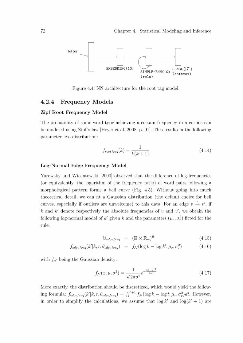
72 Chapter 4. Statistical Modeling and Inference
letter
EMBEDDING(10)SIMPLE-RNN(10)(relu)
DENSE(|T |)(softmax)
Figure 4.4: NN architecture for the root tag model.
4.2.4 Frequency Models
Zipf Root Frequency Model
The probability of some word type achieving a certain frequency in a corpus canbe modeled using Zipf’s law [Heyer et al. 2008, p. 91]. This results in the followingparameter-less distribution:
frootfreq(k) =1
k(k + 1)(4.14)
Log-Normal Edge Frequency Model
Yarowsky and Wicentowski [2000] observed that the difference of log-frequencies(or equivalently, the logarithm of the frequency ratio) of word pairs following amorphological pattern forms a bell curve (Fig. 4.5). Without going into muchtheoretical detail, we can fit a Gaussian distribution (the default choice for bellcurves, especially if outliers are unwelcome) to this data. For an edge v r→ v′, ifk and k′ denote respectively the absolute frequencies of v and v′, we obtain thefollowing log-normal model of k′ given k and the parameters (µr, σ2
r) fitted for therule:
Θedgefreq = (R× R+)R (4.15)
fedgefreq(k′|k, r, θedgefreq) = fN (log k − log k′;µr, σ2r) (4.16)
with fN being the Gaussian density:
fN (x;µ, σ2) =1√
2πσ2e−(x−µ)2
2σ2 (4.17)
More exactly, the distribution should be discretized, which would yield the follow-ing formula: fedgefreq(k′|k, r, θedgefreq) =
∫ k′+1k′ fN (log k − log t;µr, σ2
r)dt. However,in order to simplify the calculations, we assume that log k′ and log(k′ + 1) are

4.2. Model Components 73
−8 −6 −4 −2 0 2 4 6 8
0
0.1
0.2
0.3
0.4
Landen:Landes
Kreuzen:Kreuzes
abrupten:abruptes
dichten:dichtes kurzen:kurzes
fertigen:fertiges
gleichen:gleiches
log k − log k′
Pro
babi
lity
dens
ity
Figure 4.5: The difference in log-frequencies between words on the left and rightside of the rule /Xen/ → /Xes/ in German. The dashed line is the best-fittingGaussian density.
sufficiently close that the Gaussian density at both those points is roughly equal.
4.2.5 Word Embedding Models
The inclusion of word embeddings in the model is motivated by the observationthat some morphological transformations (e.g. plural or comparative formation)correspond to a regular shift of the word vector [Mikolov et al. 2013b].
Gaussian Root Vector Model
The simplest way to model our uncertainty about some vectors of real values isto use a multivariate Gaussian distribution. The string form of the word is nottaken into account. The model is then defined by the formulas given below, withθrootvec = 〈µ, σ2〉, both µ and σ2 being d-dimensional vectors.
Θrootvec = Rd × Rd+ (4.18)
frootvec(x|v, θrootvec) = fMN (x;µ, diag(σ2)) (4.19)
with fMN being the multivariate Gaussian density:
fMN (x;µ,Σ) =1√
det(2πΣ)e−12 (x−µ)Σ−1(x−µ) (4.20)

74 Chapter 4. Statistical Modeling and Inference
letter
EMBEDDINGSIMPLE-RNN(relu)
DENSE(tanh)
DENSE(linear)
Figure 4.6: NN architecture for the root vector model.
As the components of an embedding vector are the outcome of dimensionalityreduction, it is reasonable to assume their independence of each other. Thus, weuse a diagonal covariance matrix, which simplifies the calculations significantly.
Gaussian Edge Vector Model
The underlying assumption of the Gaussian edge vector model is that applying arule r to a word with embedding vector x yields a shifted vector x+µr, where µr isthe constant shift attributed to the rule. The difference between the observed andthe expected vector is modeled as a Gaussian variable with zero mean and varianceσ2. In order to avoid overfitting (especially for rare rules), the variance is global tothe whole model, rather than local for each rule. Thus, θedgevec = 〈{µr : r ∈ R}, σ2〉.This yields the following model:
Θedgevec = (Rd)R × Rd+ (4.21)
fedgevec(x′|x, r, θedgevec) = fMN (x′ − x;µr, diag(σ2)) (4.22)
RNN Root Vector Model
The RNN root vector model models the distribution of embedding vectors for rootwords using the neural network architecture depicted in Fig. 4.6. The vector ispredicted from the string form of the word, which is fed to the network letter byletter.
In order to convert the predicted vector into a distribution, we again usea multivariate Gaussian distribution. The ‘error’, i.e. the difference between thepredicted and the observed vector, is modeled as a Gaussian variable with zeromean and covariance matrix diag(σ2). The model parameters θedgevec thus consistof the weights of the network and the variance vector σ2.

4.3. Inference 75
x
r id
EMBEDDING(100)
DENSE(linear)
Figure 4.7: NN architecture for the edge vector model.
Neural Network Edge Vector Model
The NN edge vector model (Fig. 4.7) is a way to model more sophisticated trans-formations carried out on word embeddings by morphological rules. The input tothe network is the vector of the source word, as well as the rule, which is embeddedinto a 100-dimensional vector space. The predicted output vector is computed bya single linear layer from both those values. In this way, instead of simple addition,more sophisticated ways of combining both values can be represented. The differ-ence between the predicted and the observed vector is modeled as above, with azero-mean Gaussian.
4.3 Inference
The inference methods on the model presented here are based on sampling fromthe distribution of graph edges, as the edges are a latent variable. In general,this problem fits into the framework of learning in presence of hidden data, whichis formulated as follows: let X be the observed data, Y be the latent variablecorresponding to the hidden data, and θ be the model parameter. The modeldefines the joint distribution P (X, Y |θ). If X and Y are discrete, like in the caseof graph structures, the likelihood is expressed as follows:
L(θ;X) = P (X|θ) =∑Y
P (X, Y |θ) (4.23)
A usual goal is finding a parameter θ that maximizes the likelihood. This canbe achieved by the Expectation Maximization (EM) algorithm [Dempster et al.1977], which is based on the statement that maximizing the likelihood of the ob-

76 Chapter 4. Statistical Modeling and Inference
served data is equivalent to maximizing the following expected value:
EY |X,θ logP (X, Y |θ) (4.24)
The maximization can be achieved by picking a θ0 at random and iterating thefollowing computation:
θi = arg maxθ
EY |X,θi−1 logP (X, Y |θ) (4.25)
In many cases, computing the expected value directly is not possible, becauseit requires summing over all possible values of Y , which might be computationallyprohibitive. Therefore, sampling approaches are often used to approximate the ex-pectation. In particular, Markov chain Monte Carlo (MCMC) methods, that com-pute the next point of the sample from the previous point, are useful for complexmodels.
Sec. 4.3.1 contains a theoretical introduction to MCMC methods with focuson the Metropolis-Hastings (MH) algorithm. In Sec. 4.3.2, I develop a samplerbased on the MH algorithm which can be used to draw samples of morphologygraphs in the model presented in Sec. 4.1. As some model components may requirenegative examples, i.e. possible edges leading to non-existent vertices, for fitting,I describe a method of sampling such examples in Sec. 4.3.3. The graph samplercan be used for optimizing the model parameters (Sec. 4.3.4), as well as for modelselection, i.e. finding the optimal set of morphological rules needed to explain thedata (Sec. 4.3.5). Section 4.3.6 briefly mentions a different inference procedure,which is based on finding a single best graph, instead of computing expectations.
4.3.1 MCMC Methods and the Metropolis-Hastings Algo-
rithm
The following introduction is based on Robert and Casella [2005]. Some definitionsand theorems contain references to their direct counterparts in the source work.The proofs of the theorems are skipped here, as they can be found in the references.However, for the purposes of this thesis, we will consider only the case of Markovchains with a finite state space. This is sufficient for our applications and greatlysimplifies the presentation of the theoretical foundations.
Let X be a finite set of states and f be a probability distribution over X .In the following, we will be interested in drawing large samples x(0), x(1), . . . , x(n),which are representative of f . In particular, we will use the sample to approximate
4.3. Inference 77
expected values of the form:
Efh(X) =∑x∈X
f(x)h(x) ≈ 1n
n∑i=0
h(x(i)) (4.26)
In order to achieve a good approximation, the sample need not necessarilybe independent. In fact, we will work with samples, in which each point dependson the previous one. Such sample is the outcome of a Markov chain.
Definition 4.1. Given a transition matrix K, a sequence X0, X1, . . . , Xn, . . . ofrandom variables is a Markov chain, denoted by (Xn), if, for any t, the conditionaldistribution of Xt given Xt−1, Xt−2, . . . , X0 is the same as the distribution of Xt
given Xt−1; that is:
P (Xt|X0, X1, . . . , Xt−1) = P (Xt|Xt−1) = K(Xt−1, X) (4.27)
In the case of a finite state space,K is simply a matrix of dimensions |X |×|X |.However, I will use the notation K(x, y) instead of kxy for better readability. AsK(x, y) is the probability of a transition from x to y, it has to satisfy the condition∀x∈X
∑y∈X K(x, y) = 1
Definition 4.2. A (discrete) Markov chain (Xn) is irreducible if all states com-municate, namely if:
P (τy <∞|X0 = x) > 0 ∀x, y ∈ X (4.28)
τy being the first time y is visited.
Definition 4.3. A probability distribution π over X is called the stationary dis-tribution of a Markov chain with transition matrix K if it satisfies the followingcondition for every x ∈ X :
π(x) =∑y∈X
π(y)K(y, x) (4.29)
The stationary distribution gives the chain the following property: if Xn ∼ π,then also Xn+1 ∼ π. In particular, if X0 ∼ π, it follows by induction that all X’sare distributed according to π.
Definition 4.4. A Markov chain with transition matrix K satisfies the detailed

78 Chapter 4. Statistical Modeling and Inference
balance condition if there exists a function f satisfying:
K(y, x)f(y) = K(x, y)f(x) (4.30)
for every (x, y).
Theorem 4.5 (Robert and Casella 2005, Th. 6.46, adjusted to the finite case).Suppose that a Markov chain with transition matrix K satisfies the detailed bal-ance condition with π a probability distribution. Then, the distribution π is thestationary distribution of the chain.
Definition 4.6 (Robert and Casella 2005, Def. 7.1). A Markov chain Monte Carlo(MCMC) method for the simulation of a distribution f is any method producingan ergodic Markov chain (Xn) whose stationary distribution is f .
In great simplification, a Markov chain with finite state space is ergodic if thestationary distribution exists and is independent of the starting point. The detailsof this concept are not further relevant here, because in the following we are going toconsider one particular MCMC method. Summarizing the above introduction, thefoundation of MCMC methods is the convergence of an irreducible Markov chainto a stationary distribution, which justifies using the chain for drawing samplesfrom this distribution.
We will now turn to a very general MCMC method called the Metropolis-Hastings(MH) algorithm [Metropolis et al. 1953; Hastings 1970]. This algorithm can beused to construct a Markov chain having an arbitrary probability distribution f
as its stationary distribution. The main advantage is that sampling directly fromf is not at all necessary. Instead, sample points are sampled from an instrumentaldistribution q(·|x), which might be completely unrelated to f .
Algorithm 4.1 presents a single iteration of the MH algorithm, computingthe t+ 1-st point of the sample from the previous one. The proposed new point issampled from the instrumental distribution q(·|x(t)). Then, the algorithm decidesrandomly whether to accept it. In case of rejection, the chain stays at the currentstate.
The acceptance probability α is the key point of the algorithm, which com-bines the distributions f and q. Importantly, it does not require knowing f exactly:as it only involves ratios, it is sufficient that f is known up to a multiplicative con-stant. In case q is symmetric, i.e. q(x|y) = q(y|x), the second ratio is droppedcompletely.

4.3. Inference 79
Algorithm 4.1: A single iteration of the Metropolis-Hastings algorithm.Generate Yt ∼ q(y|x(t)) ;
α← min{f(Yt)f(x(t))
q(x(t)|Yt)q(Yt|x(t)) , 1
};
Generate U ∼ Bernoulli (α) ;if U = 1 then
x(t+1) ← Ytelse
x(t+1) ← x(t)
end
Theorem 4.7 (Robert and Casella 2005, Th. 7.2). The Markov chain induced bythe Metropolis-Hastings algorithm satisfies the detailed balance condition wrt. thetarget distribution f .
Corollary 4.8. The distribution f is stationary wrt. the Markov chain inducedby the Metropolis-Hastings algorithm.
4.3.2 A MCMC Sampler for Morphology Graphs
The graph sampler described in this section has been proposed in [Sumalvico 2017].It is inspired by similar approaches for dependency parsing [Marecek 2012; Teich-mann 2014], which also use MCMC samplers for graphs. The key idea is to con-struct a proposal distribution which conducts a small change in the graph, likeadding or removing a single edge.
Let E denote the set of all possible edges that were found in the preprocessingstep described in Sec. 3.3. We will be interested in subsets E ⊆ E forming branch-ings, i.e. directed forests. The well-formedness conditions for a branching are thatthe graph contains no cycles and every node has at most one incoming edge.
Let E(t) denote the t-th branching in the sample. We will now formulate theproposal distribution q(·|E(t)), which can be used to propose the next branching.The main idea is to choose an edge from E with uniform probability and change itsstatus in E, i.e. remove it if it is present, or add it if it is absent. Removing an edgealways preserves the branching properties: the target node of the removed edgesimply becomes a root. However, adding an edge can create a cycle or break theproperty of every node having at most one incoming edge. In this case, additionalchanges shall be proposed to repair the branching properties.
Let v1 denote the source node and v2 the target node of the edge that issupposed to be added. Furthermore, let v3 denote the current parent of v2, if it

80 Chapter 4. Statistical Modeling and Inference
v3 v2 v5 . . . v4 v1 v3 v2 v5 . . . v4 v1
Figure 4.8: The two variants of the ‘flip’ move. The deleted edges are dashed andthe newly added edges dotted. The goal of the operation is to make possible addingan edge from v1 to v2 without creating a cycle.
exists. If v2 already contains an incoming edge, but v1 is not a descendent of v2, theproposal is to add the edge v1 → v2 and remove the edge v3 → v2. Note that in somesettings, the same pair of vertices might be connected with multiple edges, labeledby different rules. In this case, v3 might be equal to v1. The procedure remains thesame: the newly added edge is simply exchanged for the current incoming edge ofv2.
If v1 is a descendent of v2, adding an edge v1 → v2 would create a cycle. Inorder to avoid that, I propose a change called ‘flip’, which is illustrated in Fig. 4.8.Here, v4 denotes the parent of v1 and v5 denotes the direct child of v2 on the pathleading to v1. As in the previous case, the overlapping of some of those nodes doesnot change the procedure. The move has two variants, each of which consisting ofadding and removing two edges. In the first variant, we ‘cut out’ v1 (together withthe whole subtree rooted in it) from its current place and insert it between v3 andv2. In the second variant, we ‘cut out’ v2 and move it (together with all its childrenexcept v5) in a proper place to be the child of v1.
Algorithm 4.2 presents the procedure for proposing the next branching. If a‘flip’ operation is required, the variant is chosen randomly with equal probability.Note that a ‘flip’ move might be impossible if the other edge to be added (v3 → v1
in the first and v3 → v5 in the second variant) is not available in E . In this case,the functions FLIP-* leave the current branching unchanged.
The choice of the next branching is uniquely determined by the choice of theedge (v1, v2, r) to be changed and, in case of the ‘flip’ move, the value of U . A movethat adds or removes a single edge can be reversed by selecting the same edge again.A move that exchanges edges can be reversed by selecting the previously removededge to be added again. Finally, each ‘flip’ move can be reversed by another ‘flip’move. FLIP-1 is reversed by selecting v4 → v1 to be added and applying FLIP-2,while variant 2 can be reversed by selecting v2 → v5 and applying FLIP-1. Inconclusion, the proposal distribution is symmetric.

4.3. Inference 81
Algorithm 4.2: Proposing the next branching in the sample.Input: E(t) – current branching; E – set of all possible edgesOutput: Y (t) – a proposal for the next branchingChoose an edge (v1, v2, r) randomly from E ;if (v1, v2, r) ∈ E(t) then
Y (t) ← E(t) \ {(v1, v2, r)} ;else if v2 is ancestor of v1 then
Generate U ∼ Bernoulli(12) ;
if U = 1 thenY (t) ← FLIP-1(E(t), E , v1, v2, r) ;
elseY (t) ← FLIP-2(E(t), E , v1, v2, r) ;
endelse if parent(v2) 6= nil then
Let v3, r′ be so that (v3, v2, r
′) ∈ E(t) ;Y (t) ← E(t) ∪ {(v1, v2, r)} \ {(v3, v2, r
′)} ;else
Y (t) ← E(t) ∪ {(v1, v2, r)} ;endreturn Y (t)
The acceptance probability is thus calculated as follows:
α∗ = exp[c(E(t))− c(Y (t))
](4.31)
= exp
∑(v1,v2,r)∈E(t)\Y (t)
c(v1, v2, r)−∑
(v1,v2,r)∈Y (t)\E(t)c(v1, v2, r)
(4.32)
with the final acceptance probability being: α = min{α∗, 1}.Note that the chain constructed this way is irreducible, because every branch-
ing can be reached from every other with nonzero (albeit very small) probabilityby first deleting all edges of the old branching and then adding all edges of thenew branching.
Proposing the next branching has very low computational complexity: O(h),where h is the maximum height of a tree in the branching. The only operation thatis not performed in constant time is checking for cycles and determining v5. If thetree height is kept low (for which, as described in Sec. 4.1.3, there are good reasons),the time complexity of proposing the next branching is as good as constant. Thisenables us to draw large samples in the order of magnitude of millions or billionsbranchings independently of |E|, and thus input data.

82 Chapter 4. Statistical Modeling and Inference
Figure 4.9: The trajectory of the graph sampler expressed as the cost (negativelog-likelihood) of the graph at a given iteration. The top plot shows all 10 millionsampling iterations, while the bottom plot shows iterations from 4 million onward.The acceptance rate in this run was 0.12.
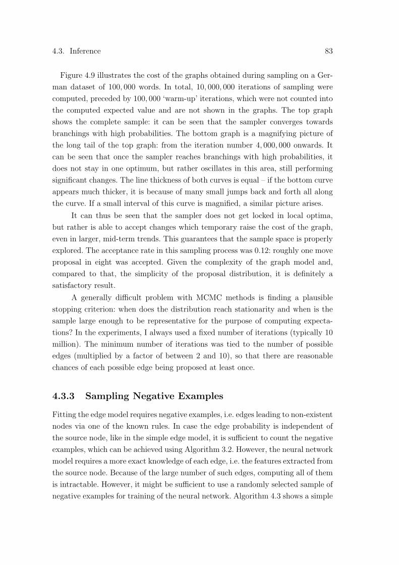
4.3. Inference 83
Figure 4.9 illustrates the cost of the graphs obtained during sampling on a Ger-man dataset of 100, 000 words. In total, 10, 000, 000 iterations of sampling werecomputed, preceded by 100, 000 ‘warm-up’ iterations, which were not counted intothe computed expected value and are not shown in the graphs. The top graphshows the complete sample: it can be seen that the sampler converges towardsbranchings with high probabilities. The bottom graph is a magnifying picture ofthe long tail of the top graph: from the iteration number 4, 000, 000 onwards. Itcan be seen that once the sampler reaches branchings with high probabilities, itdoes not stay in one optimum, but rather oscillates in this area, still performingsignificant changes. The line thickness of both curves is equal – if the bottom curveappears much thicker, it is because of many small jumps back and forth all alongthe curve. If a small interval of this curve is magnified, a similar picture arises.
It can thus be seen that the sampler does not get locked in local optima,but rather is able to accept changes which temporary raise the cost of the graph,even in larger, mid-term trends. This guarantees that the sample space is properlyexplored. The acceptance rate in this sampling process was 0.12: roughly one moveproposal in eight was accepted. Given the complexity of the graph model and,compared to that, the simplicity of the proposal distribution, it is definitely asatisfactory result.
A generally difficult problem with MCMC methods is finding a plausiblestopping criterion: when does the distribution reach stationarity and when is thesample large enough to be representative for the purpose of computing expecta-tions? In the experiments, I always used a fixed number of iterations (typically 10million). The minimum number of iterations was tied to the number of possibleedges (multiplied by a factor of between 2 and 10), so that there are reasonablechances of each possible edge being proposed at least once.
4.3.3 Sampling Negative Examples
Fitting the edge model requires negative examples, i.e. edges leading to non-existentnodes via one of the known rules. In case the edge probability is independent ofthe source node, like in the simple edge model, it is sufficient to count the negativeexamples, which can be achieved using Algorithm 3.2. However, the neural networkmodel requires a more exact knowledge of each edge, i.e. the features extracted fromthe source node. Because of the large number of such edges, computing all of themis intractable. However, it might be sufficient to use a randomly selected sample ofnegative examples for training of the neural network. Algorithm 4.3 shows a simple

84 Chapter 4. Statistical Modeling and Inference
method to generate such a sample. The number of generated edges (n) is usuallya multiple of the number of possible edges (|E|), typically twice as much.
Algorithm 4.3: Sampling negative examples of edges.Input: V,R, E , nOutput: S – a sample of random edges from outside ES ← ∅;while |S| < n do
Choose v randomly from V ;Choose r randomly from R;if r(v) 6= ∅ then
Choose v′ randomly from r(v);if (v, v′, r) /∈ S ∧ (v, v′, r) /∈ E then
S ← S ∪ {(v, v′, r)};end
endendreturn S
Because we are using only a subset of negative edges for training the neuralnetwork, they have to be weighted accordingly to the number of edges they repre-sent. If kr is the number of generated edges labeled with rule r, nr is the numberof possible edges (from E) labeled with r and mr is the total number of timesr can be applied, each negative edge obtains the weight mr−nr
kr. Algorithm 4.3 is
quite a naıve sampling approach: it is easy to see that the probability of selectinga particular edge is not uniform (as it depends on |r(v)|).
4.3.4 Fitting the Model Parameters
Using the sampler introduced in Sec. 4.3.2, we can generate samples E(1), E(2), . . .
from the conditional distribution P (E|V,R, θ). Such samples can be used to ap-proximate expected values of functions over E. This enables us to apply the MonteCarlo Expectation Maximization (MCEM) algorithm [Wei and Tanner 1990] to findthe maximum likelihood estimates of the model parameters. We aim to iterativelymaximize the following expected value (cf. 4.25):
θi = arg maxθ
EE|V,R,θi−1 logP (V,E|R, θ) (4.33)
In the expectation step, besides the global log-likelihood, we also compute theexpected relative frequency of each edge, i.e. the fraction of branchings in which

4.3. Inference 85
this edge appears. Those values constitute the edge weights used for fitting. Theroot weights can be easily obtained from the edge weights: the root weight of nodev, i.e. the fraction of branchings in which it is a root, is one minus the sum ofweights of all its incoming edges.
In the maximization step, the parameters of each model component are fitto maximize the likelihood of the sample. This is easy in case of most models.In the simple edge model, the ML estimate for rule probability is n
m, where n is
the expected frequency of the rule (in this case, the sum of weights of all edgeslabeled with this rule) and m is the number of times the rule can be applied.The latter can be computed by applying Algorithm 3.2 to the composition of thelexicon and rule transducer. The Gaussian models can be fit to weighted samplesby using weighted averages in estimation and the neural network models acceptweighted samples as training data as well. In the latter case, the fitting consists ofa complete, multi-epoch neural network training.
For fitting the neural edge model, we use the edge weights as targets, ratherthan sample weights. The training objective of the network is to predict for eachedge the probability that it is included in a branching. In order to do it correctly,we also need to generate a weighted sample of non-existent edges with the methoddescribed in Sec. 4.3.3 and include it in the training data passed to the network.
The only model that poses problems for weighted fitting is the ALERGIA rootmodel: it can only accept integer weights (interpreted as frequencies). However, theroot model does not change significantly across fitting iterations, so we skip themaximization step for it.
The initial parameter value θ0 is usually chosen randomly in the EM algo-rithm. However, in this case, we can easily guess a more-or-less reasonable value:it is the value fit to the full graph, i.e. when all edge and root weights are set to 1.We call this a ‘naıve fit’. Using this value as θ0 speeds up the convergence of thealgorithm, because we already start in a region yielding relatively high likelihood.
Figure 4.10 shows the expected branching costs (minus log-likelihoods) ob-tained during the MCEM estimation. The first iteration, which is out of scale inthe graph’s Y axis, uses the parameters obtained via naıve fitting. The algorithmconverges quickly: there is not much change after the 10th iteration, comparedto the first 10. As I could not decide for any stopping criterion, and in order tomaintain greater control of the duration of the estimation, I use a fixed number ofiterations (typically 5) in the experiments.

86 Chapter 4. Statistical Modeling and Inference
2 4 6 8 10 12 14 16 18 201.06
1.07
1.08
1.09
1.1
1.11·106
Iteration
Exp
.gr
aph
cost
Figure 4.10: Convergence of MCEM fitting. The cost at the first iteration is farbeyond the scale (around 1.6 · 106).
4.3.5 Model Selection
In addition to finding optimal parameters θ for a given rule set R, we can alsoattempt to optimize the rule set itself by deleting unnecessary rules. This wouldcorrespond to finding the following maximum:
R = arg maxR′⊆R
∫ΘEE|V,R′,θ logP (V,E|R′, θ)dθ (4.34)
In [Sumalvico 2017], I proposed to search for the optimal rule set using simu-lated annealing [Kirkpatrick et al. 1983; Besag 2004]. For each rule, a score was com-puted based on the expected contribution of this rule to the graph log-likelihood.Those scores were used to propose the next rule set, so that rules with low scoreshad smaller chances of surviving to the next iteration. Then, the expected log-likelihood of the graph given the next rule set was computed and the rule set waseither accepted or rejected.
Although this approach improved the evaluation results in [Sumalvico 2017],further experiments led to the conclusion that it is much too complicated for thebenefit that it offers. Furthermore, its theoretical foundation is dubious: becauseeach iteration requires a complete run of MCMC graph sampler, only a few iter-ations of annealing can be executed – typically up to 20, which is much too littleto expect convergence of the annealing algorithm. Finally, the integration over Θ

4.3. Inference 87
is only tractable for the simple edge model and even there it is quite complicatedto implement. Thus, I decided to abandon this approach.
Model selection can be also done in a simpler, although less theoretically soundway. To begin with, we replace the integral in (4.34) with a maximum. In thisway, we can use regular fitting and sampling to evaluate a rule set. Furthermore,instead of attempting to search for the optimal rule set, we restrict ourselves todeletion of rules that appear useless after each sampling and fitting iteration. Forthis purpose, we define the score of a rule as follows:
score(r) = − log λRPrule(r)+∑
e=(v,v′,r)∈Ewe [logProot(v′|θroot)− log pedge(v, v′, r|θedge)]
(4.35)The first term is a new model component: a rule model, defining a probabilitydistribution over arbitrary rules. We use a very simple unigram model over pairs ofinput-output symbols in the subsequent transitions of the rule’s FST. The term λR
is due to the fact that we draw sets of rules from this distribution (see Sec. 4.1.2).The second term is the log-likelihood we gain by using the rule r to derive words,rather than having those words as roots. we is the sample weight of edge e. Aftereach iteration, the rules with negative scores are deleted. The rule model introducesa cost of having an additional rule in the model, which has to be compensated bythis rule’s usefulness.
Figure 4.11 illustrates the outcomes of model selection after each iteration.The rule set is typically reduced to roughly half its original size. The edges la-beled with the deleted rules are also deleted from E . The number of possible edgesdecreases more slowly than the number of rules because the deleted rules are typi-cally infrequent. However, the set E of possible edges is also substantially reduced.For most experiments, evaluation results are virtually unaffected by model selec-tion, but the net benefit of applying it is a smaller model, and therefore fastercomputation times.
4.3.6 Finding Optimal Branchings
Previous sections described drawing large samples of branchings and using themto estimate model parameters. This corresponds to the variant of the ExpectationMaximization algorithm often called ‘soft EM’, which utilizes full expected values.Another commonly used variant is ‘hard EM’ [Samdani et al. 2012], in whichthe inference would be based on a single optimal graph. Although I previously

88 Chapter 4. Statistical Modeling and Inference
0 2 4 6 8 10 12 14 16 18 200
2,000
4,000
6,000
8,000
Iteration
rule
s
0
0.2
0.4
0.6
0.8
1·106
edge
s
rules edges
Figure 4.11: The number of rules and possible edges during model selection.
experimented with the hard-EM algorithm [Janicki 2015], I found that taking asingle optimal graph is insufficient. Especially for rare rules, the difference betweenfrequencies 0, 1 or 2 was very significant, but no intermediary values were possible.However, as the edge costs in the model are local and independent of each other,the optimum branching can be found using Chu-Liu-Edmonds algorithm [Tarjan1977].

Chapter 5
Learning Inflectional Relations
In order to assess the practical usability of the model described in the previouschapter, I evaluate it on several different tasks related to inflection. Although themorphology learning method developed in this thesis is not especially targetedtowards inflection – in fact, the evaluation results of the unsupervised experimentspresented in this chapter suffer from the confusion of inflection and derivation,which is a consequence of Whole Word Morphology’s theoretical assumptions –there are practical reasons for evaluating the quality of inflectional analysis.
The first and most important reason is that inflectional analysis is a well-defined task. In the most common formulation, it consists of assigning a lemmaand an inflectional tag (a bundle of values of inflectional features, like case, number,person etc.) to words in text. This chapter concentrates especially on lemmatiza-tion and related tasks, like generating inflected forms from lemmas or identifyinginflected forms of the same lemma. For such kind of problems, methods basedon string transformations on word types seem appropriate. Inflectional taggingrequires a different kind of approach: it is best done on the token basis, takingthe local context of a token into account. A method targeting the tagging task incombination with morphology is presented in Chap. 6.
Another reason for an evaluation on inflection-related tasks is the availabil-ity of datasets. Lemmatized and tagged corpora are easily available. In contrast,there is no standardized task and annotation scheme for learning derivation, orinflection combined with derivation, especially in a relational formulation, i.e. fo-cusing on relations between words, rather than internal word structure.1 Finally,
1The tree annotation provided by the CELEX lexical database [Baayen et al. 1995] comesclose to being the right annotation for this kind of problems. Unfortunately, it is only availablefor three closely related languages (English, German and Dutch), all exhibiting a fairly simpleinflectional and derivational morphology.
89
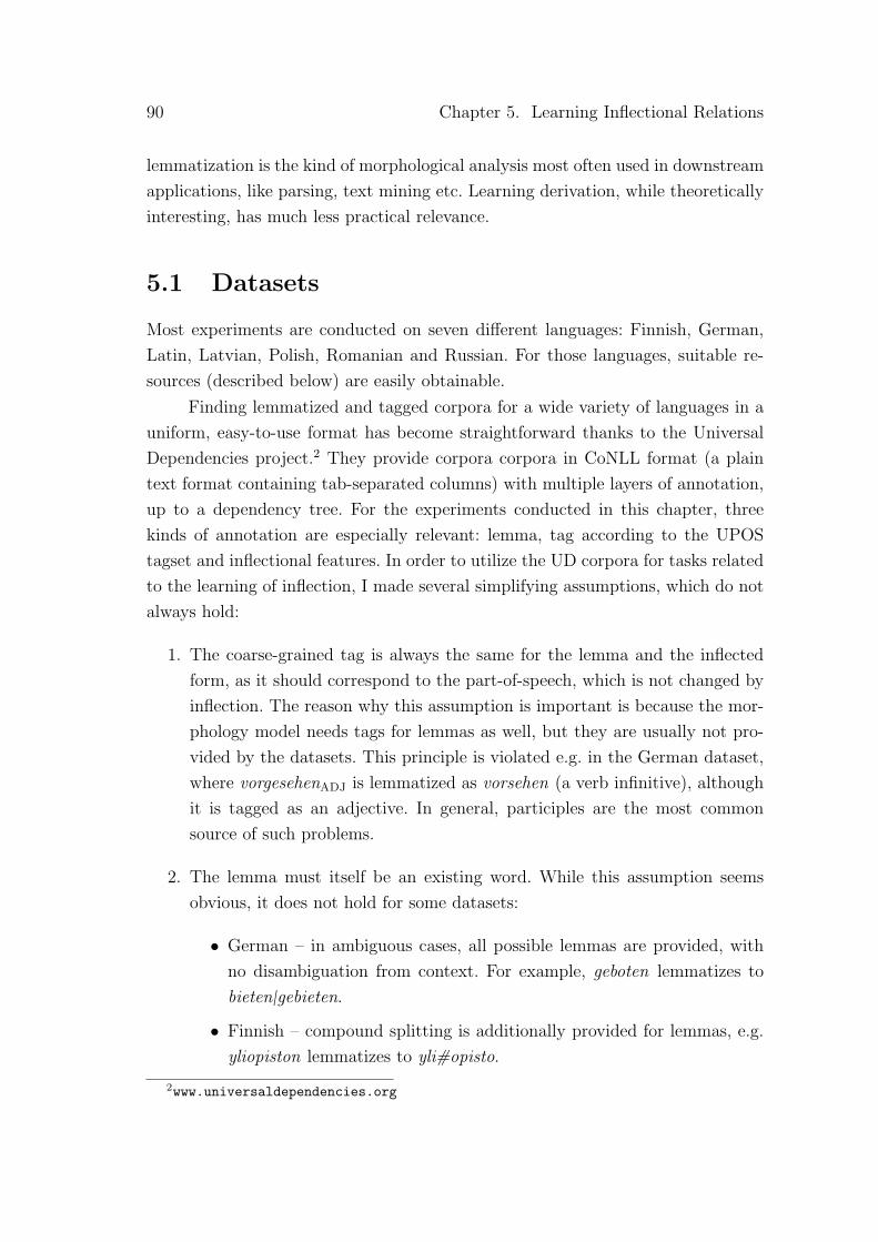
90 Chapter 5. Learning Inflectional Relations
lemmatization is the kind of morphological analysis most often used in downstreamapplications, like parsing, text mining etc. Learning derivation, while theoreticallyinteresting, has much less practical relevance.
5.1 Datasets
Most experiments are conducted on seven different languages: Finnish, German,Latin, Latvian, Polish, Romanian and Russian. For those languages, suitable re-sources (described below) are easily obtainable.
Finding lemmatized and tagged corpora for a wide variety of languages in auniform, easy-to-use format has become straightforward thanks to the UniversalDependencies project.2 They provide corpora corpora in CoNLL format (a plaintext format containing tab-separated columns) with multiple layers of annotation,up to a dependency tree. For the experiments conducted in this chapter, threekinds of annotation are especially relevant: lemma, tag according to the UPOStagset and inflectional features. In order to utilize the UD corpora for tasks relatedto the learning of inflection, I made several simplifying assumptions, which do notalways hold:
1. The coarse-grained tag is always the same for the lemma and the inflectedform, as it should correspond to the part-of-speech, which is not changed byinflection. The reason why this assumption is important is because the mor-phology model needs tags for lemmas as well, but they are usually not pro-vided by the datasets. This principle is violated e.g. in the German dataset,where vorgesehenADJ is lemmatized as vorsehen (a verb infinitive), althoughit is tagged as an adjective. In general, participles are the most commonsource of such problems.
2. The lemma must itself be an existing word. While this assumption seemsobvious, it does not hold for some datasets:
• German – in ambiguous cases, all possible lemmas are provided, withno disambiguation from context. For example, geboten lemmatizes tobieten|gebieten.
• Finnish – compound splitting is additionally provided for lemmas, e.g.yliopiston lemmatizes to yli#opisto.
2www.universaldependencies.org

5.2. Unsupervised Clustering of Inflected Forms 91
• Latin – additional disambiguation information is provided for lemmas,e.g. occides lemmatizes to occido#1.
While the latter two cases seem to provide useful additional information,the proper conversion of the datasets would require some effort and exper-tise – e.g. on the first sight it is unclear whether the Finnish lemmas canalways be converted to real words just by deleting the separator, or whetherthe distinction in Latin data is relevant to morphology or only semantic. Ingeneral, I decided against language-specific preprocessing and excluded thoselanguages from lemmatization experiments.
3. A word that is lemma of other words is also its own lemma, i.e. lemmatiza-tion does not form chains or cycles. This is again violated in German, e.g.vorgeseheneADJ is lemmatized to vorgesehen, but vorgesehenADJ to vorsehen.Other datasets contain similar cases.
As a source of plain, unannotated corpora employed for fully unsupervised train-ing, I utilize the Leipzig Corpora Collection3 [Biemann et al. 2007]. For the mostlanguages, the standard-sized corpora of 1 million sentences coming from Wikipediaare used. Exceptions are Latin, where the full Wikipedia is used, and Latvian,where a 1 million sentence corpus of news crawled from the Internet is used in-stead. Both exceptions are due to small sizes of Wikipedias in those languages(both around 300k sentences).
5.2 Unsupervised Clustering of Inflected Forms
Given only an unannotated corpus or a list of words, the only kind of inflectionalanalysis that can be realistically expected is the clustering of inflected forms comingfrom the same lemma. As the choice of a certain inflectional form as citation formis more or less arbitrary (e.g. verb infinitive in many languages, but 1st personsingular in Latin and Greek, 3rd person singular in Hungarian etc.), it is, in myopinion, not possible to establish reliable criteria allowing for automatic discoveryof lemmas.4
3corpora.uni-leipzig.de4Attempts have been made to determine the lemma based on, for example, the frequency of
inflectional categories [Chan 2008] or efficiency of a grammar deriving inflected forms from alemma [Albright 2002]. However, the former concentrates on identifying some base form, fromwhich other forms can be derived, but which is not necessarily the lemma accepted in the lan-guage’s grammar. The latter concentrates on theoretical linguistic aspects and does not provide

92 Chapter 5. Learning Inflectional Relations
Experiment setup. In order to identify clusters of morphologically relatedwords (which will mostly be different inflected forms of the same lemma), I employthe Chinese Whispers graph clustering algorithm [Biemann 2006].
As weights of the edges in the morphology graph, I use the expected edgefrequencies determined during sampling. They have a useful property: the sumof weights of all incoming edges in a node, plus the expected frequency of thatnode being a root, equals one. In other words, the incoming edges are mutuallyexclusive events. This gives a straightforward probabilistic interpretation to theweight-adding done by Chinese Whispers: it corresponds to the event of the parentnode of the considered node being in a certain cluster. Furthermore, the event of anode being a root is treated as a loop edge: it contributes its weight to the proposalof staying in the current cluster. In this way, nodes that have incoming edges canstill remain singletons (which would have been impossible without loops).
The experiments were carried out in several different variants in order toassess the influence of various model configurations on the overall performance.All experiments employ the ALERGIA root model. The labels ‘single’ and ‘neural’correspond to the edge model used, ‘-freq’ to an additional frequency model and‘-emb’ to an additional word embedding model (word embeddings with 30 dimen-sions were trained with word2vec). The models used for embeddings were the onesbased on neural networks, Gaussian models were left out of the evaluation.
All experiments consisted of 5 iterations of model selection followed by an-other 5 iterations of fitting. A single sampling step consisted of 100,000 warm-upiterations and 10,000,000 sampling iterations while training. The final sampling,which determines the expected frequencies of edges using the trained model, con-tained 100,000,000 sampling iterations. Apart from the variants using an embed-ding model, all other variants used a parameter α = e−2 to control the tree height(see Sec. 4.1.3). The variants with embeddings used no such functionality (i.e.α = 1), as the tree height is sufficiently limited by the expensive, unpredictablechanges in word embeddings.
Experiments for all languages were done using the same parameter values,which were mostly guessed before the experiments as reasonable defaults. I delib-erately avoided the fine-tuning of parameters to each dataset separately.
Baselines. As I am not aware of any publicly available algorithm implementationsolving exactly the same task, the usefulness of the approach developed here will bedemonstrated through a comparison to simple baselines. The most naıve approach
empirical results on corpora.

5.2. Unsupervised Clustering of Inflected Forms 93
possible is to place every word in a separate cluster, which is called ‘bl-singleton’.The other baseline, ‘bl-logfreq’, consists of applying the Chinese Whispers algo-rithm to a morphology graph, in which the edges are weighted by the logarithmfrequency of the rule. This roughly corresponds to the approach taken by Janicki[2013].5
Evaluation measure. As a clustering evaluation measure, I use BCubed [Amigóet al. 2009], which provides results in the usual form of precision, recall and F1-score. Note that the reason why ‘bl-singleton’ sometimes achieves apparently goodresults (especially for German) is that the gold standard contains many singletonclusters. For once, many rare words occur in the corpus only in one inflected form.Furthermore, there are many types, which do not correspond to real words of thelanguage (e.g. numbers, foreign words, abbreviations etc.). I deliberately did notexclude such cases from the test data.
Results. The results are shown in Table 5.1. In general, no consistent improve-ment over the ‘bl-logfreq’ baseline can be observed. The results range from a sig-nificant improvement (Latvian, Russian) over slight improvement (German, Ro-manian), no difference (Polish) up to a slight decrease (Latin). On the other hand,the good performance of the singleton baseline for German is an exception, as forall other datasets this baseline performs poorly.
Most results suffer from low precision, meaning that the clusters tend to betoo large. The main reason for this is the inability of the model to distinguishbetween inflection and derivation. Especially in cases where there is not enough in-flected forms to form a stable cluster, words related through derivation are clusteredtogether instead. However, in Latin, a language with particularly large inflectionalparadigms, a contrary trend is observed: some paradigms are so large that they aresplit into several clusters. A further reason for low precision are accidental similar-ities between short words. The probabilistic model helps to rule out some of suchpatterns (especially through model selection), but not all of them. Such similaritiescan form ‘bridges’ between unrelated clusters, leading to their merging.
No significant difference can be observed between the simple and the neural
5Janicki [2013] contained an additional step consisting of clustering the outgoing edges ofeach node and splitting nodes according to edge clusters. This step greatly improved the results(especially precision). However, it is a feature of the clustering algorithm, which could be appliedregardless of the weighting. The main point of the evaluation provided here is to compare theweights obtained in sampling to log-frequencies, so the details of the clustering algorithm areorthogonal to this comparison.

94 Chapter 5. Learning Inflectional Relations
Language Model Prec. Rec. F1
German
bl-singleton 100.0 % 81.2 % 89.6 %bl-logfreq 70.5 % 97.4 % 81.8 %simple 78.6 % 95.9 % 86.4 %simple-freq 77.7 % 96.2 % 86.0 %neural 77.9 % 95.9 % 86.0 %simple-emb 70.8 % 97.0 % 81.9 %neural-emb 69.6 % 97.3 % 81.1 %
Latin
bl-singleton 100.0 % 27.9 % 43.7 %bl-logfreq 74.4 % 74.0 % 74.2 %simple 80.0 % 61.1 % 69.3 %simple-freq 79.1 % 61.7 % 69.3 %neural 80.3 % 61.2 % 69.5 %simple-emb 67.3 % 67.7 % 67.5 %neural-emb 68.5 % 67.4 % 68.0 %
Latvian
bl-singleton 100.0 % 48.2 % 65.0 %bl-logfreq 46.5 % 80.2 % 58.9 %simple 76.8 % 82.9 % 79.7 %simple-freq 76.2 % 82.6 % 79.3 %neural 77.1 % 83.5 % 80.1 %simple-emb 69.4 % 86.5 % 77.0 %neural-emb 69.2 % 87.0 % 77.1 %
Polish
bl-singleton 100.0 % 47.7 % 64.6 %bl-logfreq 76.0 % 86.0 % 80.7 %simple 81.2 % 80.4 % 80.8 %simple-freq 80.7 % 80.8 % 80.7 %neural 81.0 % 80.5 % 80.7 %simple-emb 80.6 % 80.8 % 80.7 %neural-emb 80.7 % 80.7 % 80.7 %
Romanian
bl-singleton 100.0 % 50.0 % 66.7 %bl-logfreq 73.0 % 92.0 % 81.4 %simple 79.5 % 87.8 % 83.4 %simple-freq 78.3 % 88.4 % 83.0 %neural 79.8 % 88.3 % 83.8 %simple-emb 71.5 % 90.0 % 79.7 %neural-emb 71.9 % 90.2 % 80.0 %
Russian
bl-singleton 100.0 % 34.7 % 51.6 %bl-logfreq 51.8 % 76.3 % 61.7 %simple 78.5 % 84.8 % 81.5 %simple-freq 76.4 % 85.2 % 80.6 %neural 78.2 % 84.8 % 81.4 %simple-emb 68.7 % 86.1 % 76.4 %neural-emb 70.3 % 85.8 % 77.3 %
Table 5.1: Results of unsupervised clustering.

5.3. Unsupervised Lemmatization 95
edge model, as well as between the variant with and without a frequency model.The models with word embeddings perform slightly worse because of their lack ofpenalty on tree height – the assumption that using the embeddings as an additionalfeature can restrict the tree height equally well, does not hold.
5.3 Unsupervised Lemmatization
As justified in the previous section, I do not think that a completely unsupervisedlemmatization is possible, as the choice of lemmas is to a certain degree arbitrary.However, an experiment with very little supervision is possible: in addition to anunlemmatized corpus, we provide the algorithm with a list of lemmas. The list isnot necessarily complete: lemmas for some forms from the corpus may be missing.The task of the algorithm is to assign the inflected forms from the corpus to thecorrect lemma from the provided list (if the correct lemma is available), then tolearn lemmatizing rules from those assignments and finally to apply the learnt rulesto generate missing lemmas.
Experiment setup. I use whole Universal Dependencies corpora for both train-ing and testing. For training, the list of unlemmatized types from the corpus isprovided, either without part-of-speech tags or with coarse-grained tags. The listof lemmas provided additionally contains only words that themselves appear inthe corpus as tokens, so a fair amount of lemmas is missing. For training, I usethe ‘left and right’ restrictions described in Sec. 3.3.4: only edges leading from alemma to an inflected form (i.e. a form appearing in the corpus which is not itselfa lemma) are allowed. I use the ALERGIA root model and either simple or neuraledge model. For the experiments with tagged data, the simple root tag model isused.
Back-formation. A trained model can generate missing lemmas through back-formation. The idea is that the root cost (i.e. the negative log-probability accordingto the distribution Proot) of an inflected form might be larger that the cost of alemma plus the cost of an edge deriving the inflected form from the lemma. Thisis especially likely if POS tags are used: the training data contain mostly rootswith tags characteristic to lemmas, so the distribution Proottag will attribute highprobabilities to such tags and very low probabilities to tags characteristic to in-flected forms. Therefore, for each inflected form that is supposed to be lemmatized,the learnt rules are applied to generate all possible lemmas. The cost of an edge

96 Chapter 5. Learning Inflectional Relations
corresponding to each rule is computed. Furthermore, if the lemma is not presentin the training vocabulary, its cost as a root is added to the cost of the analysis.Formally:
lemma(v) = arg minr∈R
v′∈r−1(v)
[− ln pedge(v′, v, r|θedge)− (1− 1V (v′)) lnProot(v′|θroot)]
(5.1)1V (·) is the indicator function of set V , i.e. 1 if the argument belongs to V and0 otherwise. In case a tagged model is used, the last term must be additionallymultiplied by Proottag(t′|v′, θroottag).
Baseline. The baseline of this experiment consists of extracting candidate rulesbetween lemmas and inflected forms and using the most frequent rule for eachform to match it to a lemma. Inflected forms, for which no rules are extracted (e.g.because the true lemma is missing) are left unmatched. Using the most frequentrule is superior to using the rule with minimum edit distance, because the lattermethod would be prone to accidental word similarities (like substituting the firstletter) which are not common patterns.
Results. The evaluation results are shown in Table 5.2. While the results onuntagged datasets are mixed, on tagged datasets at least the simple edge modelprovides a consistent slight improvement (with the exception of Latvian, wherethe result is equal to the baseline). The neural edge model performs in generalsignificantly worse. This is not surprising: in the unsupervised setting, where thetraining data are not reliable, a more flexible model runs more into the risk ofoverfitting to wrong examples.
5.4 Supervised Lemmatization
In the supervised lemmatization experiment, a lemmatized corpus is split intotwo parts: the training and testing data. The training corpus is used to learn amorphology model, which is then applied to lemmatize words from the testingcorpus. For supervised training, we use the method described in Sec. 3.3.4.
For the experiments described in this section, 30% of the corpus (more ex-actly: the first 30% running tokens)6 is taken as training data. From the remaining
6The split is deterministic on purpose. A random split would have made the evaluation muchmore expensive, because each experiment would have to be repeated multiple times. As the split
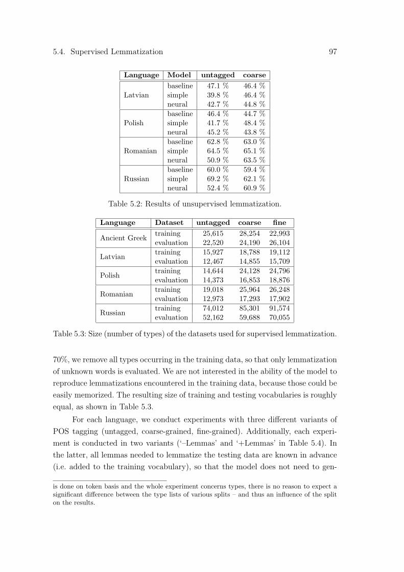
5.4. Supervised Lemmatization 97
Language Model untagged coarse
Latvianbaseline 47.1 % 46.4 %simple 39.8 % 46.4 %neural 42.7 % 44.8 %
Polishbaseline 46.4 % 44.7 %simple 41.7 % 48.4 %neural 45.2 % 43.8 %
Romanianbaseline 62.8 % 63.0 %simple 64.5 % 65.1 %neural 50.9 % 63.5 %
Russianbaseline 60.0 % 59.4 %simple 69.2 % 62.1 %neural 52.4 % 60.9 %
Table 5.2: Results of unsupervised lemmatization.
Language Dataset untagged coarse fine
Ancient Greektraining 25,615 28,254 22,993evaluation 22,520 24,190 26,104
Latviantraining 15,927 18,788 19,112evaluation 12,467 14,855 15,709
Polishtraining 14,644 24,128 24,796evaluation 14,373 16,853 18,876
Romaniantraining 19,018 25,964 26,248evaluation 12,973 17,293 17,902
Russiantraining 74,012 85,301 91,574evaluation 52,162 59,688 70,055
Table 5.3: Size (number of types) of the datasets used for supervised lemmatization.
70%, we remove all types occurring in the training data, so that only lemmatizationof unknown words is evaluated. We are not interested in the ability of the model toreproduce lemmatizations encountered in the training data, because those could beeasily memorized. The resulting size of training and testing vocabularies is roughlyequal, as shown in Table 5.3.
For each language, we conduct experiments with three different variants ofPOS tagging (untagged, coarse-grained, fine-grained). Additionally, each experi-ment is conducted in two variants (‘–Lemmas’ and ‘+Lemmas’ in Table 5.4). Inthe latter, all lemmas needed to lemmatize the testing data are known in advance(i.e. added to the training vocabulary), so that the model does not need to gen-
is done on token basis and the whole experiment concerns types, there is no reason to expect asignificant difference between the type lists of various splits – and thus an influence of the spliton the results.

98 Chapter 5. Learning Inflectional Relations
erate lemmas on its own, only choose the right one. The former case correspondsto ‘normal’ supervised training, i.e. nothing from the testing dataset is known inadvance. In this case, the model attempts to generate the missing lemmas throughback-formation. The model configurations used in the experiments are same as inthe previous section.
Baseline. Supervised lemmatization can be formulated as a classification prob-lem, as shown for example by Chrupała et al. [2008]. In this formulation, the classis the lemmatizing rule (or, equivalently, the rule deriving the inflected form fromthe lemma). The features used to predict the class are the word’s POS tag andletter n-grams.
As the system described by Chrupała et al. [2008] was geared towards jointlemmatization and POS tagging, it would have been incompatible with my exper-iments: it operated on token basis and made use of local context features. Instead,I apply a heavily simplified version of this approach as baseline: I use a MaximumEntropy classifier7 to predict the word’s lemmatizing rule from the POS tag (ifpresent) and n-grams at the beginning and at the end of the word of lengths from1 to 5. In order to restrict the number of features to a manageable size, I use the1000 most frequent n-grams.
Results. The type-based accuracy of various setups is shown in Table 5.4. Apartfrom the untagged case without knowing lemmas in advance, all setups clearlyoutperform the baseline. The former case shows that an unlabeled string form of aword is usually not enough for reliable lemmatization. The presence of POS-tags,even coarse-grained, improves the situation significantly.
As in other experiments, also here it turns out that the neural edge modeloffers no benefit over the simple edge model. This is unexpected, as the greaterflexibility of the neural model ought to be an advantage especially in supervisedlearning, where tighter fitting of the model to the training examples is beneficial.
The results for Ancient Greek are a clear outlier. Perhaps the most importantreason for this is the polytonic orthography, which, together with accent shifts inmorphological paradigms, greatly complicates the inflection.8 Moreover, the An-cient Greek verb morphology is complicated compared to other considered lan-guages: the paradigms are large and many possible transformations are rare or not7More specifically, I use the classifier LogisticRegression implemented in the Python pack-
age scikit-learn. This is identical to the baseline I used in [Janicki 2015].8In addition to accent shifts in morphological paradigms, even the same word form can occur
with different accent types depending on its context in the sentence [Smyth 1920, p. 37].

5.5. Supervised Inflected Form Generation 99
present in training data at all. Also suppletion seems to be more common thanin the other languages. Finally, it seems to me that some irregularities are due tonon-standard historical spellings: for example, the word Θρῄκης ‘Thrace.gen’ islemmatized as Θρᾴκη, instead of Θρῄκη postulated by the model. Wiktionary9 ex-plains that the former is the standard form and the latter is a ‘poetic’ variant. Theannotators of the corpus seemingly decided to use standard spellings for lemmas incases where inflected forms are spelled in a non-standard way. This is understand-able from the point of view of corpus annotation, but it makes inflection appearmore irregular than it actually is.
In the variant where the lemmas are not known in advance (the left halfof the table), the results with fine-grained tags are significantly higher than forcoarse-grained tags. It turns out that coarse-grained tags are not enough to lem-matize properly as inflectional affixes may be ambiguous. For example, the Polishmasculine animate noun kot ‘cat’ has following forms: kot ‘cat-nom.sg’, kota ‘cat-gen.sg’, koty ‘cat-nom.pl’. Compare this to the paradigm of lina ‘rope’, which isa feminine noun: lina ‘rope-nom.sg’, liny ‘rope-gen.sg’, lin ‘rope-gen.pl’. Thus,only knowing that the word is a noun ending in -a does not provide enough clueto determine the lemma.
The right half of the table shows the results in the case where all lemmas areknown in advance. The results illustrate an important difference between my modeland the baseline classifier: there is no straightforward way to make the classifierbenefit from knowing the lemmas in advance. On the other hand, my model directlybenefits from it by changing the costs computed by (5.1) accordingly, which hasa high impact on the performance. Thus, the graph-based model provides an easyway to boost up the accuracy of the lemmatizer by feeding it with additional lexicalresources.
5.5 Supervised Inflected Form Generation
Inflected form generation is the reverse of lemmatization: given a lemma and desiredtag, for example (machen<VERB>, <VERB><PART>), the model is supposed to producethe suitable inflected form, in this case gemacht. As the desired inflected form hasto be exactly specified, only fine-grained tags make sense in this context. Then,the learnt rules are used to generate all possible inflections from the given lemmas.
9https://en.wiktionary.org/wiki/%CE%98%CF%81%E1%BF%84%CE%BA%CE%B7 accessed onDec 11, 2018.

100 Chapter 5. Learning Inflectional Relations
Language Model–Lemmas +Lemmas
untagged coarse fine untagged coarse fine
AncientGreek
baseline 26.2 % 30.9 % 35.5 % 26.2 % 31.0 % 35.4 %simple 24.0 % 33.2 % 35.6 % 36.2 % 41.7 % 39.2 %neural 23.1 % 25.4 % 32.0 % 35.0 % 40.1 % 39.0 %
Latvianbaseline 52.1 % 61.5 % 71.7 % 52.3 % 61.3 % 72.0 %simple 45.0 % 60.7 % 77.2 % 76.8 % 83.7 % 80.3 %neural 47.7 % 56.8 % 74.8 % 76.6 % 83.4 % 80.1 %
Polishbaseline 54.0 % 60.9 % 69.2 % 54.1 % 60.9 % 69.1 %simple 55.1 % 69.9 % 79.2 % 81.6 % 87.7 % 82.7 %neural 57.3 % 63.1 % 77.1 % 82.3 % 87.5 % 82.7 %
Romanianbaseline 57.7 % 70.7 % 74.3 % 58.4 % 70.4 % 74.1 %simple 61.4 % 74.0 % 82.7 % 83.1 % 92.5 % 90.6 %neural 64.2 % 72.1 % 81.9 % 83.7 % 92.3 % 90.6 %
Russianbaseline 60.2 % 65.7 % 74.9 % 60.1 % 65.7 % 75.0 %simple 58.5 % 72.0 % 79.1 % 80.4 % 87.5 % 84.9 %neural 57.9 % 69.6 % 78.6 % 80.9 % 87.5 % 84.6 %
Table 5.4: Results of supervised lemmatization.
The obtained list is filtered to include only the entries matching the desired POStag.
The baseline is similar to the one used in the previous experiment: a maximumentropy classifier utilizing prefix and suffix character n-grams and POS tag. Thedifference is that the n grams are now extracted from the lemma, while the tagused for classification is the tag of the desired word.
Results The results of the experiment are shown in Table 5.5. Because of theproblems described in the previous section, Ancient Greek was excluded from thisexperiment. The results show a slight advantage of my model (especially with thesimple edge model) over the baseline, with the exception of Russian. Bearing inmind that the Russian corpus is significantly larger than others, this differencemight be a characteristic of the size of the training data rather than language.Nevertheless, the results of all methods are similar.
Note that while a classifier has to be trained for each task separately, thegraph-based models used to solve this task are exactly the same as those usedfor lemmatization. It is satisfactory to see that a general model of ‘morphologicalcompetence’ achieves similar, or even slightly better scores, than baseline modelsdedicated to a single task.

5.5. Supervised Inflected Form Generation 101
Language Model Accuracy
Latvianbaseline 70.9 %simple 73.4 %neural 72.4 %
Romanianbaseline 85.8 %simple 88.9 %neural 84.1 %
Polishbaseline 80.1 %simple 82.8 %neural 81.5 %
Russianbaseline 87.0 %simple 85.4 %neural 84.9 %
Table 5.5: Results of supervised inflected form generation.

102 Chapter 5. Learning Inflectional Relations

Chapter 6
Semi-Supervised Learning ofPOS Tagging
Part-of-speech tagging is nowadays commonly thought of as a solved problem, withaccuracy scores easily achieving 95% or more. However, such results are typicallyreported for English or other resource-rich European languages, for which largeamounts of high-quality training data are available. Those languages also tendto have a simple morphology and utilize small to mid-sized tagsets. However, formany other languages, the reality is different: training data are expensive or notavailable, more fine-grained tagsets are needed and complex morphology accountsfor large numbers of OOV words in corpora. Straka and Strakova [2017] presenta contemporary evaluation of state-of-the-art POS tagging for a very wide varietyof languages. The scores for tagging with UPOS1 tagset lie below 90% for manylanguages. The lack of sufficient amounts of training data is undoubtedly one ofthe main reasons for such results.
In this chapter, I attempt to improve the POS tagging in a setting whereonly a small amount of labeled training data is available, as well as a significantlylarger corpus of unlabeled text. I train a bigram Hidden Markov Model on thelabeled part of the corpus and subsequently apply Baum-Welch estimation on theunlabeled part. Additionally, I use the labeled corpus to learn morphological rules,which are then applied to guess the possible tags of the words from the unlabeledpart. For the latter step, I modify the graph sampler developed in Sec. 4.3.2 totreat the unknown tags as latent features which influence edge probabilities.
The choice of a bigram HMM for tagging is clearly suboptimal. However,
1The tagset used in the Universal Dependencies project. It is very coarse-grained, containinge.g. only a single tag for nouns and verbs, respectively.
103
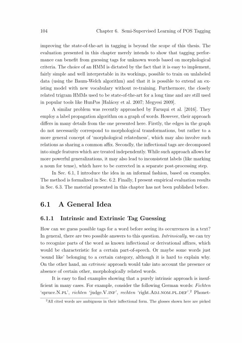
104 Chapter 6. Semi-Supervised Learning of POS Tagging
improving the state-of-the-art in tagging is beyond the scope of this thesis. Theevaluation presented in this chapter merely intends to show that tagging perfor-mance can benefit from guessing tags for unknown words based on morphologicalcriteria. The choice of an HMM is dictated by the fact that it is easy to implement,fairly simple and well interpretable in its workings, possible to train on unlabeleddata (using the Baum-Welch algorithm) and that it is possible to extend an ex-isting model with new vocabulary without re-training. Furthermore, the closelyrelated trigram HMMs used to be state-of-the-art for a long time and are still usedin popular tools like HunPos [Halacsy et al. 2007; Megyesi 2009].
A similar problem was recently approached by Faruqui et al. [2016]. Theyemploy a label propagation algorithm on a graph of words. However, their approachdiffers in many details from the one presented here. Firstly, the edges in the graphdo not necessarily correspond to morphological transformations, but rather to amore general concept of ‘morphological relatedness’, which may also involve suchrelations as sharing a common affix. Secondly, the inflectional tags are decomposedinto single features which are treated independently. While such approach allows formore powerful generalizations, it may also lead to inconsistent labels (like markinga noun for tense), which have to be corrected in a separate post-processing step.
In Sec. 6.1, I introduce the idea in an informal fashion, based on examples.The method is formalized in Sec. 6.2. Finally, I present empirical evaluation resultsin Sec. 6.3. The material presented in this chapter has not been published before.
6.1 A General Idea
6.1.1 Intrinsic and Extrinsic Tag Guessing
How can we guess possible tags for a word before seeing its occurrences in a text?In general, there are two possible answers to this question. Intrinsically, we can tryto recognize parts of the word as known inflectional or derivational affixes, whichwould be characteristic for a certain part-of-speech. Or maybe some words just‘sound like’ belonging to a certain category, although it is hard to explain why.On the other hand, an extrinsic approach would take into account the presence orabsence of certain other, morphologically related words.
It is easy to find examples showing that a purely intrinsic approach is insuf-ficient in many cases. For example, consider the following German words: Fichten‘spruce.N.pl’, richten ‘judge.V.inf’, rechten ‘right.Adj.nom.pl.def’.2 Phonet-2All cited words are ambiguous in their inflectional form. The glosses shown here are picked

6.1. A General Idea 105
ically and orthographically they are very similar and all include an inflectionalsuffix -en, which is highly ambiguous in German. The knowledge that Germannouns are always capitalized does not provide much of a clue, because wordsbelonging to any other part-of-speech may also occur capitalized. Even worse,many further similar words are ambiguous in their meaning and part-of-speech,e.g. Dichten (‘density.N.pl’ or capitalized ‘dense.Adj.nom.pl.def’ or ‘compose(e.g. a poem).V.inf’), schlichten (‘simple.Adj.nom.pl.def’ or ‘mediate.V.Inf’).
The situation becomes diametrically different if we take into account mor-phologically related words. For example, we might observe words like richtet orrichtete, which together with richten look unambiguously like a verb paradigm.Similarly, the occurrence of a form like rechtes can convince us that rechten is anadjective, because verbs do not take the suffix -es. For ambiguous forms, we willlikely find parts of different paradigms, for example schlichtet (verb) and schlichtes(adjective), which will allow us to notice the ambiguity. Of course, in order to con-duct such analysis, we have to know which affix configurations are characteristicfor which part of speech. This is the part that we are going to learn from labeleddata.
6.1.2 Applying Tagged Rules to Untagged Words
Let us assume that we have learned a morphology model on tagged data. Now weare presented with a new set of words, possibly containing many words not presentin the original training set. In this section, we will show how the trained model canbe applied to derive guesses for tags in the new vocabulary. The approach followsthe idea sketched in the previous section: the tag of the word will be determinedby the neighboring words, together with the knowledge about the morphologycontained in tagged rules.
To illustrate the approach with a minimal example, let us assume that ourtagset consists of only three tags:NN,VVINF andVVFIN, and that the untaggedvocabulary consists of the German words machen, mache, macht. We compute theedge probabilities for every edge that is possible according to the model, underevery tagging. For example, the model might determine that the following threeedges are possible (i.e. the corresponding tagged rules are included in the model)
as examples.

106 Chapter 6. Semi-Supervised Learning of POS Tagging
(a) machen mache
macht
(b) machen mache
macht
/Xen/ → /Xe/ /Xen/ → /Xe/
/Xen/ → /Xt/
Figure 6.1: Two possible morphology graphs corresponding to the words machen,mache, macht. What does each of them tell us about the possible tags of thosewords according to (6.1)?
and give following probabilities for them:
pedge(machenNN,macheNN, /Xen/NN → /Xe/NN) = 0.3
pedge(machenVVINF,macheVVFIN, /Xen/VVINF → /Xe/VVFIN) = 0.01 (6.1)
pedge(machenVVINF,machtVVFIN, /Xen/VVINF → /Xt/VVFIN) = 0.2
Using those values, we can reason about the possible taggings based on an untaggedgraph. Consider the two graphs shown in Fig. 6.1. What does each of them sayabout the possible taggings?
Graph 6.1a is consistent with either {machenNN, macheNN} or {machenVVINF,macheVVFIN}, since the only edge in this graph is possible with both labelings. Notethat the edge containing noun labels has much higher probability, so this graphsuggests a strong preference for the noun hypothesis. It does not say anythingabout the possible tags of macht. On the other hand, the only tagging consistentwith the graph 6.1b is {machenVVINF, macheVVFIN, machtVVFIN}, since the edgebetween machen and macht is only possible if machen is a verb infinitive. It isimportant to notice that adding an edge between machen and macht diametricallychanged the possible taggings for mache, although it is not touched by the edgein question. This illustrates how the graph model captures dependencies betweenthe tags across a whole paradigm, although the edge probabilities are local.
6.2 The Method
Recall from Sec. 4.1.4 that a morphology model trained on tagged data defines aprobability distribution P (V, T,E|R, θ) over tagged graphs, consisting of words V ,edges E and tag assignments T = {Tv : v ∈ V }, given the rulesR and model param-eters θ. The tags of root nodes are predicted by a distribution Proottag(t|v, θroottag),which takes into account the string form of the word, v, and distribution parametersθroottag.
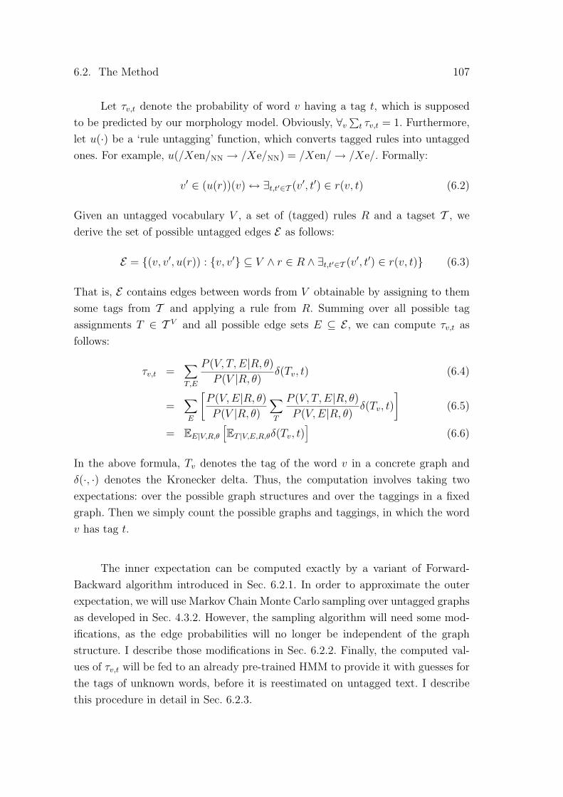
6.2. The Method 107
Let τv,t denote the probability of word v having a tag t, which is supposedto be predicted by our morphology model. Obviously, ∀v
∑t τv,t = 1. Furthermore,
let u(·) be a ‘rule untagging’ function, which converts tagged rules into untaggedones. For example, u(/Xen/NN → /Xe/NN) = /Xen/→ /Xe/. Formally:
v′ ∈ (u(r))(v)↔ ∃t,t′∈T (v′, t′) ∈ r(v, t) (6.2)
Given an untagged vocabulary V , a set of (tagged) rules R and a tagset T , wederive the set of possible untagged edges E as follows:
E = {(v, v′, u(r)) : {v, v′} ⊆ V ∧ r ∈ R ∧ ∃t,t′∈T (v′, t′) ∈ r(v, t)} (6.3)
That is, E contains edges between words from V obtainable by assigning to themsome tags from T and applying a rule from R. Summing over all possible tagassignments T ∈ T V and all possible edge sets E ⊆ E , we can compute τv,t asfollows:
τv,t =∑T,E
P (V, T,E|R, θ)P (V |R, θ)
δ(Tv, t) (6.4)
=∑E
[P (V,E|R, θ)P (V |R, θ)
∑T
P (V, T,E|R, θ)P (V,E|R, θ)
δ(Tv, t)]
(6.5)
= EE|V,R,θ[ET |V,E,R,θδ(Tv, t)
](6.6)
In the above formula, Tv denotes the tag of the word v in a concrete graph andδ(·, ·) denotes the Kronecker delta. Thus, the computation involves taking twoexpectations: over the possible graph structures and over the taggings in a fixedgraph. Then we simply count the possible graphs and taggings, in which the wordv has tag t.
The inner expectation can be computed exactly by a variant of Forward-Backward algorithm introduced in Sec. 6.2.1. In order to approximate the outerexpectation, we will use Markov Chain Monte Carlo sampling over untagged graphsas developed in Sec. 4.3.2. However, the sampling algorithm will need some mod-ifications, as the edge probabilities will no longer be independent of the graphstructure. I describe those modifications in Sec. 6.2.2. Finally, the computed val-ues of τv,t will be fed to an already pre-trained HMM to provide it with guesses forthe tags of unknown words, before it is reestimated on untagged text. I describethis procedure in detail in Sec. 6.2.3.
108 Chapter 6. Semi-Supervised Learning of POS Tagging
v1 v2 v3 v4 v5 v6 v7 v8 v9
Figure 6.2: The Forward-Backward computation for a linear sequence in an HMM.αv6,t = P (v1, . . . , v6, T6 = t), whereas βv6,t = P (v7, v8, v9|T6 = t).
6.2.1 The Forward-Backward Algorithm for Trees
In order to compute τv,t = ET |V,E,R,θδ(Tv, t) for a fixed graph (V,E), let us recall thewell-known Forward-Backward algorithm used for Hidden Markov Models.3 TheHMMs employed for POS tagging operate on sentences, which are linear sequencesof words (Fig. 6.2). The summing over all possible tag sequences is tackled byintroducing the so-called forward probability (usually written as α) and backwardprobability (β), which are defined as follows:
αvi,t = P (v1, . . . , vi, Ti = t) (6.7)
βvi,t = P (vi+1, . . . , vn|Ti = t) (6.8)
It is easy to see that the product of both, αvi,tβvi,t, gives us the probability ofthe whole sequence and the node vi having tag t. This can be used to derive τvi,t:
τvi,t =αvi,tβvi,t∑t′ αvi,t′βvi,t′
(6.9)
The point of forward-backward computation is that, due to the Markov prop-erty of HMMs, the forward and backward probability can be computed with recur-sive formulas, thus avoiding the combinatorial explosion caused by summing overall possible tag sequences:
αvi,t =∑t′αvi−1,t′P (t|t′)P (vi|t) (6.10)
βvi,t =∑t′P (t′|t)P (vi+1|t′)βvi+1,t′ (6.11)
The general idea of forward-backward computation can be extended beyondlinear sequences, which are a special case of trees, to arbitrary trees.4 In this case,the backward probability of a node is the probability of the subtree rooted in it,
3See for example Manning and Schutze [1999] or Jelinek [1997] for an introduction to HMMsand the Forward-Backward algorithm.4I was unable to find any publications describing a generalization of Forward-Backward com-
putation to tree models. I do not believe that this is my innovation, though. I would be gratefulfor any hints on this topic from reviewers and readers.
6.2. The Method 109
v1
v2
v3
v4
v5
v6
v7
v8
v9
Figure 6.3: The Forward-Backward computation for a tree. Also here, αv6,t =P (v1, . . . , v6, T6 = t) and βv6,t = P (v7, v8, v9|T6 = t).
given a tag, while the forward probability is the probability of the rest of the treeand the tag (Fig. 6.3). Note that the forward probability involves not only thepath leading from the root to the node in question (v1, v2, v4, v6 in Fig. 6.3), butalso all side branches sprouting from this path (v3, v5).
In order to derive recursive formulas similar to (6.10)–(6.11) for the tree case,let us introduce a concept of transition matrix in this case. A transition matrixT (v,v′,r) associated with an untagged edge (v, v′, r) is a matrix corresponding toedge probabilities for every possible tagging of the source and target node. Morespecifically:
T(v,v′,u(r))t,t′ =
pedge(v, t, v′, t′, r)1− pedge(v, t, v′, t′, r)
(6.12)
Continuing the example from 6.1.2, the probabilities in (6.1) yield the follow-ing transition matrix:
T (machen,mache,/Xen/→/Xe/) =
NN VVINF VVFIN
NN0.3
1−0.3 0 0VVINF 0 0 0.01
1−0.01
VVFIN 0 0 0
(6.13)
Furthermore, let λv,t be the probability that the node v with tag t is a leaf,i.e. it has no outgoing edges. This value can be computed as follows:5
λv,t =∏r∈R
∏(v′,t′)∈r(v,t)
[1− pedge(v, t, v′, t′, r)] (6.14)
5Two things can be said about the λ-values: they are extremely expensive to compute, becausethey involve a product over all hypothetical edges, also those leading to non-existent words, andthey are of virtually no importance, since they tend to differ only slightly from tag to tag. As theterms of the product are mostly numbers very close to 1, although they are many, the result isstill going to be fairly close to 1. Thus, although I include this value in the formulas for the sakeof soundness of the theory, I actually ignored it in experiments, setting λv,t = 1 everywhere.
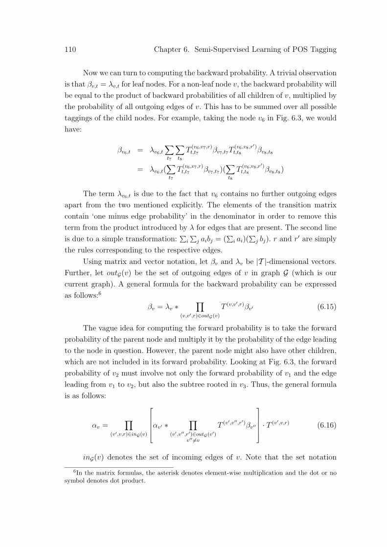
110 Chapter 6. Semi-Supervised Learning of POS Tagging
Now we can turn to computing the backward probability. A trivial observationis that βv,t = λv,t for leaf nodes. For a non-leaf node v, the backward probability willbe equal to the product of backward probabilities of all children of v, multiplied bythe probability of all outgoing edges of v. This has to be summed over all possibletaggings of the child nodes. For example, taking the node v6 in Fig. 6.3, we wouldhave:
βv6,t = λv6,t∑t7
∑t8
T(v6,v7,r)t,t7 βv7,t7T
(v6,v8,r′)t,t8 βv8,t8
= λv6,t(∑t7
T(v6,v7,r)t,t7 βv7,t7)(
∑t8
T(v6,v8,r′)t,t8 βv8,t8)
The term λv6,t is due to the fact that v6 contains no further outgoing edgesapart from the two mentioned explicitly. The elements of the transition matrixcontain ‘one minus edge probability’ in the denominator in order to remove thisterm from the product introduced by λ for edges that are present. The second lineis due to a simple transformation:
∑i
∑j aibj = (
∑i ai)(
∑j bj). r and r′ are simply
the rules corresponding to the respective edges.
Using matrix and vector notation, let βv and λv be |T |-dimensional vectors.Further, let outG(v) be the set of outgoing edges of v in graph G (which is ourcurrent graph). A general formula for the backward probability can be expressedas follows:6
βv = λv ∗∏
(v,v′,r)∈outG(v)
T (v,v′,r)βv′ (6.15)
The vague idea for computing the forward probability is to take the forwardprobability of the parent node and multiply it by the probability of the edge leadingto the node in question. However, the parent node might also have other children,which are not included in its forward probability. Looking at Fig. 6.3, the forwardprobability of v2 must involve not only the forward probability of v1 and the edgeleading from v1 to v2, but also the subtree rooted in v3. Thus, the general formulais as follows:
αv =∏
(v′,v,r)∈inG(v)
αv′ ∗ ∏(v′,v′′,r′)∈outG(v′)
v′′ 6=v
T (v′,v′′,r′)βv′′
· T (v′,v,r) (6.16)
inG(v) denotes the set of incoming edges of v. Note that the set notation
6In the matrix formulas, the asterisk denotes element-wise multiplication and the dot or nosymbol denotes dot product.

6.2. The Method 111
and the outer product is only for notational convenience, as the set is always asingleton. In this case, it means: ‘pick v′, that is the parent node of v’. The innerproduct goes over all children of v′ except for v and includes the edges leading tothem and the probabilities of the subtrees rooted in them. Finally, the last productcorresponds to the edge leading from v′ to v.
The last remaining issue is the forward probability of root nodes. It is simplyequal to the probability of the root node defined by the model, which we call ρv,tand compute as follows:
ρv,t = Proot(v|θroot)Proottag(t|v, θroottag) (6.17)
Thus, αv = ρv for root nodes.
6.2.2 Modifications to the Sampling Algorithm
As we have seen in the analysis of Fig. 6.1, adding an edge typically has conse-quences for the whole subtree, in which the edge is added. The values τv for allnodes in the subtree may change, which in turn changes the probability of all edgesin the subtree. This behavior constitutes a significant difference compared to thegeneral sampling algorithm, in which the edge probabilities were independent ofthe graph structure and the cost of a change could be easily computed from thecost of added and removed edges (cf. 4.32). Nevertheless, we can apply the samesampler as the one developed in Sec. 4.3.2.
Observe that for every node v, the value∑t αv,tβv,t is the probability of whole
subtree, to which v belongs. This property – being able to compute the probabilityof a whole subgraph using the values of a single node – is crucial in evaluating thesampler moves.
Adding or removing a single edge. Consider the graph in Fig. 6.4, to whichthe edge (v, v′, r) is supposed to be added. Without this edge, we have two separatetrees with a total probability expressed by (
∑t αv,tβv,t)(
∑t αv′,tβv′,t). After adding
this edge, we obtain a single tree. As v obtains a new child node, βv will change.Let β′v denote the new value, which can be computed as follows:
β′v = βv ∗ T (v,v′,r)βv′ (6.18)
Note that neither αv nor βv′ is affected by adding this edge. The probability of thenew tree is simply
∑t αv,tβ
′v,t. If the move is accepted, the β values of all nodes on

112 Chapter 6. Semi-Supervised Learning of POS Tagging
.
.
.
v
.
v′
.
.
.
.
..
r
Figure 6.4: Adding or removing the edge (v, v′, r).
the path from the root to v have to be updated, as well as the α values of all nodesexcept for this path.
Deleting an edge involves a very similar computation. In this case, the prob-ability of the graph before deletion is
∑t αv,tβv,t, whereas the probability after
deletion is (∑t αv,tβ
′v,t)(
∑t ρv′,tβv,t). Here, β′v,t is the updated backward probability
of v excluding the deleted edge.
Other moves. When exchanging a single edge to another one with the sametarget node, we already need to be careful, as two distinct cases arise: either thechange takes place within one tree, or it involves two separate trees (Fig. 6.5).If we proceeded as in the previous paragraph, those cases would require differentformulas. Instead of conducting such a detailed analysis of the changes, we applya more general (and, admittedly, more computationally expensive) approach, thatcovers the ‘flip’ moves as well.
First, we group all edges that are to be changed (added or deleted) accordingto the tree, to which they belong (more specifically, according to the root of thetree, to which the edge’s source node currently belongs). In each tree, we look for aminimum subtree that contains all the changes (Fig. 6.6). We build a copy of thissubtree with all changes applied and recompute the forward probability for its rootand the backward probabilities for the whole subtree. Finally, we use the (newlycomputed) forward and backward probability of the subtree root to determine theprobability of the whole tree after changes.
Note that the ‘flip’ move can change the root of a tree (Fig. 6.7). It is thusimportant to correctly recognize the root of the modified tree and to recomputeits forward probability, as it changes is this case.
A note on numerical issues. As the computation of acceptance probabilitiesnow involves probabilities of whole trees, the numbers are typically very small.Furthermore, the occurrence of addition and dot product in formulas means that

6.2. The Method 113
(a) .
v3
v1
v2
(b) .
v3
v1
v2
Figure 6.5: Exchanging an edge to another with the same target node. The changecan take place within one tree (a) or involve two separate trees (b).
.
v3
.
v2
.
v5
v4
.
v1
.
..
Figure 6.6: In case of a ‘flip’ move, the smallest subtree containing all changes is theone rooted in v3. The deleted edges are dashed, while the newly added edges aredotted. In order to obtain the new βv3 , we recompute the backward probabilitiesin the whole subtree. αv3 is not affected by the changes. (The node labels areconsistent with the definition in Fig. 4.8.)
(a) v2 v1 (b) v1 v2
Figure 6.7: A special case of the ‘flip’ move, which changes the root of the tree.(a) – the tree before the move (the edge to delete is dashed, while the edge to beadded is dotted); (b) – the tree after the move. The node labels agree with theones in Fig. 4.8, with v4 = v2, v5 = v1 and v3 not existing. The difference betweenthe two variants of ‘flip’ is neutralized in this case.

114 Chapter 6. Semi-Supervised Learning of POS Tagging
the operations cannot be carried out on log-probabilities instead. This means thatat some point (with sufficiently large trees) the floating point computations willeventually result in zeros, although in theory the tree probability is nonzero.
If a probability of the proposed graph is zero, it does not pose much of aproblem: such graph simply will not be accepted, as the acceptance probabilitywill be zero. A problem arises if the probability of the current graph turns outto be zero. In this case, we obtain a zero in the denominator of the formula foracceptance probability (see Algorithm 4.1) regardless of the proposed tree. Thissituation can arise when multiplying the probabilities of two separate trees. Eventhough probabilities of both trees are nonzero (otherwise they would not have beenaccepted), their product may be zero, i.e. smaller than the machine epsilon.7 Tosolve this problem, we introduce an artificial bound on the probability of trees:trees with a total probability smaller than some ε are never accepted. ε is chosento be at least the square root of the machine epsilon, so the product of probabilitiesof two trees is still always greater than 0.
6.2.3 Extending an HMM with New Vocabulary
The guessed tag probabilities τv,t are fed to a Hidden Markov Model before re-estimating its parameters on untagged text. Recall that an HMM possesses threekinds of parameters: initial probabilities (probability of starting in a given state),transition probabilities (probability of a state given the previous state) and emis-sion probabilities (probability of emitting a certain output symbol given the currentstate). Only the emission probabilities are affected by the extension of the vocab-ulary.
The emission probabilities in an HMM are the probabilities8 P (w|t) of aword w given a tag t. First, we convert the values in an already trained HMM toprobability of tag given a word, i.e. P (t|w), using the Bayes formula:
P (t|w) =P (w|t)P (t)∑t′ P (w|t′)P (t′)
(6.19)
7The machine epsilon is the smallest number greater than zero that can be represented as afloating-point number at a given precision. When using double precision, like the type float64in the NumPy library, this number equals 5 · 10−324.8This presentation takes a shortcut by calling HMM parameters directly probabilities. I as-
sumed that the reader is already familiar with HMMs and statistical modeling in general, so noconfusion should arise. However, such simplifications should be used with caution, especially whenintroducing statistical models, because they can obscure the understanding of what probabilityactually is.
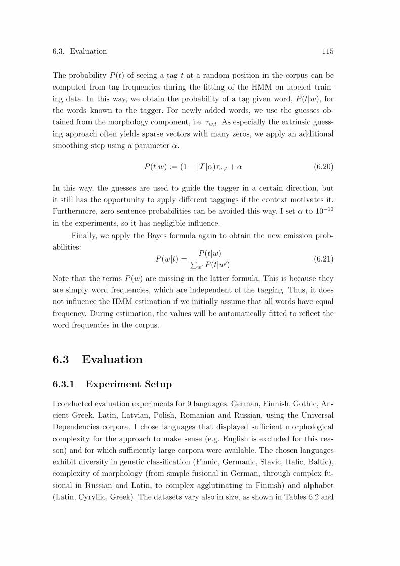
6.3. Evaluation 115
The probability P (t) of seeing a tag t at a random position in the corpus can becomputed from tag frequencies during the fitting of the HMM on labeled train-ing data. In this way, we obtain the probability of a tag given word, P (t|w), forthe words known to the tagger. For newly added words, we use the guesses ob-tained from the morphology component, i.e. τw,t. As especially the extrinsic guess-ing approach often yields sparse vectors with many zeros, we apply an additionalsmoothing step using a parameter α.
P (t|w) := (1− |T |α)τw,t + α (6.20)
In this way, the guesses are used to guide the tagger in a certain direction, butit still has the opportunity to apply different taggings if the context motivates it.Furthermore, zero sentence probabilities can be avoided this way. I set α to 10−10
in the experiments, so it has negligible influence.
Finally, we apply the Bayes formula again to obtain the new emission prob-abilities:
P (w|t) =P (t|w)∑w′ P (t|w′)
(6.21)
Note that the terms P (w) are missing in the latter formula. This is because theyare simply word frequencies, which are independent of the tagging. Thus, it doesnot influence the HMM estimation if we initially assume that all words have equalfrequency. During estimation, the values will be automatically fitted to reflect theword frequencies in the corpus.
6.3 Evaluation
6.3.1 Experiment Setup
I conducted evaluation experiments for 9 languages: German, Finnish, Gothic, An-cient Greek, Latin, Latvian, Polish, Romanian and Russian, using the UniversalDependencies corpora. I chose languages that displayed sufficient morphologicalcomplexity for the approach to make sense (e.g. English is excluded for this rea-son) and for which sufficiently large corpora were available. The chosen languagesexhibit diversity in genetic classification (Finnic, Germanic, Slavic, Italic, Baltic),complexity of morphology (from simple fusional in German, through complex fu-sional in Russian and Latin, to complex agglutinating in Finnish) and alphabet(Latin, Cyryllic, Greek). The datasets vary also in size, as shown in Tables 6.2 and

116 Chapter 6. Semi-Supervised Learning of POS Tagging
1 Fitting on the training set.2 1 + estimation on the development set.3 2 + extension of the vocabulary with random initialization.4 2 + extension of the vocabulary with intrinsic tag guesses.5 2 + extension of the vocabulary with extrinsic tag guesses.6 2 + extension of the vocabulary with gold standard tag guesses.
Table 6.1: Different setups of the HMM tagger used in the tagging experiment.
6.3.Each corpus is randomly split into training, development and testing dataset
in proportions 10%:80%:10%. An HMM tagger is fitted to the (labeled) trainingdata using ML estimation. The training dataset is also used to learn tagged mor-phological rules. Then, we remove the labels from the development corpus andre-estimate the HMM on this corpus using Baum-Welch algorithm. This step isperformed in several configurations: either with or without vocabulary expansion.In the latter case, all types occurring in the development corpus, but not knownto the HMM (i.e. not occurring in the training corpus) are added to the vocabu-lary before the estimation. Finally, the tagging accuracy is assessed on the testingdataset. The details of the possible configurations are shown in Table 6.1.
For each corpus, two kinds of datasets are prepared: with coarse-grained andfine-grained tags. In the former case, the UPOS tagset is used, which amounts toaround 15 tags for every language. In the latter, all inflectional information pro-vided by the corpus annotation is additionally included. For example, in the Latincorpus, we have tokens like beati<ADJ> in the coarse-grained and beati<ADJ><NOM><POS><MASC><PLUR> in the fine-grained case.
The extrinsic tag guessing approach developed in the previous section is com-pared to intrinsic guesses. Those are provided directly by the distribution Proottag,which, in this case, uses a character-based recurrent neural network to predict theword’s tag from its string form (see Sec. 4.2.3).
6.3.2 Evaluation Measures
Two kinds of evaluation are performed: lexicon and tagging evaluation. In the firstcase, the quality of tag guesses for unknown words, τv, is measured directly. Itis desirable for those values to not only predict the correct tag for unambiguouswords, but also to handle ambiguity correctly, which means providing probabilitiesthat correspond to the expected frequency of a word with the certain tag. Wederive the gold standard data from the labels in the development set using the

6.3. Evaluation 117
following formula:τv,t =
nv,t∑t′ nv,t′
(6.22)
with nv,t being the number of occurrences of word v with tag t in the developmentset. This way, true ambiguities (with roughly equal frequency of different taggings)are treated differently than rare taggings, which may result from tagging errors orsome obscure, infrequent meanings. The accuracy is computed as follows:
accuracy =1|V |
∑v∈V
∑t
min{τv,t, τv,t} (6.23)
It is intentionally a very demanding measure: it achieves 100% for a given wordonly if the probability mass is distributed exactly according to the corpus frequencyof the tagging variants, which is virtually impossible for ambiguous words. Hence,low scores according to this measure are not surprising and do not necessarilyrepresent a bad-quality tagging. I decided for this measure, because it is easier tointerpret than e.g. KL-divergence.
In the tagging evaluation, we evaluate the impact of providing tag guesseson a real POS-tagging task. The evaluation measure used there is the standardaccuracy, i.e. the percentage of correctly tagged tokens.
6.3.3 Results
Tables 6.2 and 6.3 show the results of the lexicon evaluation, as well as someinformation about the sizes of the datasets. The first three columns show thenumber of distinct tags found in the training set, the size (number of types) of thetraining set and the size of the development set. Note that the sizes for the samelanguage in both tables differ slightly: firstly, fine-grained tags would yield moretypes from the same corpus because of more possible taggings per word. Secondly,the tables describe distinct experiments with different random splits of the data.Thus, the datasets in Table 6.3 are typically slightly larger, but the reverse case isalso possible.
The results show clearly that the extrinsic method outperforms the intrinsicin predicting possible tags for a given word type. Probably the most importantreason for that is that the intrinsic method always makes unsharp predictions –it never attributes the whole probability mass to a single tag. On the other hand,the extrinsic method often makes unambiguous predictions because of the absenceof rules allowing for alternatives (a phenomenon illustrated in Fig. 6.1). Thus, the
118 Chapter 6. Semi-Supervised Learning of POS Tagging
Language #tags #train #devel Intrinsic ExtrinsicAncient Greek 14 7.7k 34k 60.7 % 66.0 %Finnish 15 10k 49k 50.7 % 64.3 %German 16 10k 45k 61.6 % 67.6 %Gothic 13 2.1k 7.6k 48.3 % 66.1 %Latin 14 7k 26k 54.4 % 70.4 %Latvian 17 5.1k 23k 50.6 % 64.6 %Polish 15 5.6k 28k 58.7 % 69.5 %Romanian 16 7.8k 30k 54.0 % 70.5 %Russian 16 30k 110k 68.2 % 76.9 %
Table 6.2: Lexicon evaluation with coarse-grained tags.
Language #tags #train #devel Intrinsic ExtrinsicAncient Greek 481 8.2k 34k 22.9 % 30.0 %Finnish 906 10k 48k 25.5 % 41.1 %German 519 11k 45k 15.4 % 21.0 %Gothic 333 2k 7.7k 15.7 % 30.8 %Latin 632 7.5k 26k 23.6 % 44.8 %Latvian 501 5.1k 23k 24.0 % 36.8 %Polish 394 5.9k 28k 19.6 % 31.5 %Romanian 185 7.7k 30k 24.1 % 30.1 %Russian 597 33k 110k 33.0 % 52.2 %
Table 6.3: Lexicon evaluation with fine-grained tags.

6.3. Evaluation 119
Language 1 2 3 4 5 6Ancient Greek 66.9 % 74.2 % 73.2 % 78.9 % 79.1 % 85.7 %Finnish 60.6 % 74.4 % 72.8 % 79.5 % 82.3 % 83.8 %German 77.1 % 75.5 % 83.1 % 84.9 % 85.1 % 83.6 %Gothic 76.8 % 77.0 % 80.3 % 81.9 % 82.8 % 86.5 %Latin 74.3 % 80.8 % 81.6 % 82.5 % 86.6 % 85.6 %Latvian 67.0 % 72.3 % 73.1 % 79.6 % 80.3 % 84.8 %Polish 71.5 % 78.7 % 74.5 % 78.1 % 84.2 % 82.9 %Romanian 78.5 % 84.6 % 85.3 % 88.0 % 88.4 % 87.0 %Russian 80.9 % 87.7 % 87.7 % 90.3 % 90.5 % 91.4 %
Table 6.4: Tagging evaluation with coarse-grained tags.
latter achieves better scores especially on correctly tagged unambiguous words.
The comparison of tagging accuracies is shown in Tables 6.4 and 6.5. Thecolumns correspond to the tagger configurations explained in Table 6.1. In general,a rise of the score from left to right is to be expected.
The difference between columns 1 and 2 illustrates the influence of reesti-mating the trained model on unlabeled data without adding the OOV words tothe vocabulary. Interestingly, this results in an improvement in case of the coarse-grained tagset, but in a decline when using the fine-grained tagset, both significant.However, adding the OOV words from the development set to the vocabulary, evenwith randomly initialized probabilities (column 3), further improves the accuracy(with a few exceptions), so that the result is consistently better than column 1.Column 4 introduces intrinsic tag guessing as initial probabilities for newly addedwords, rather than random values. This results in a further improvement, espe-cially significant for Finnish, Ancient Greek and Latvian (both coarse-grained andfine-grained).
The most important comparison in this evaluation is between column 4 and5. This illustrates the benefit of using extrinsic tag guessing (column 5), ratherthan intrinsic. This results in a consistent improvement, ranging from very slightto significant. The most significant improvements are shown in bold. Finally, col-umn 6 displays what one might expect to be the upper bound on the accuracy: theone that would be achieved if tags were guessed perfectly (i.e. as τv). Surprisingly,it is not always the highest value in a row. It looks as if taking into account somewrong taggings during Baum-Welch estimation could accidentally improve the es-timation, because the wrong tag might also have occurred in the given context.This seems especially plausible for cases like common and proper nouns, which areoften confused. However, any speculation in such a case is not of much value.

120 Chapter 6. Semi-Supervised Learning of POS Tagging
Language 1 2 3 4 5 6Ancient Greek 56.6 % 46.4 % 56.9 % 62.8 % 63.8 % 69.9 %Finnish 53.5 % 37.7 % 56.7 % 65.1 % 67.5 % 71.7 %German 59.4 % 49.8 % 58.7 % 61.8 % 62.0 % 63.1 %Gothic 63.6 % 55.0 % 65.9 % 67.7 % 67.8 % 73.9 %Latin 59.0 % 49.3 % 61.7 % 66.0 % 68.7 % 73.4 %Latvian 58.5 % 47.1 % 59.4 % 65.7 % 66.8 % 71.3 %Polish 55.4 % 43.7 % 57.5 % 62.5 % 62.7 % 67.9 %Romanian 71.2 % 71.3 % 75.9 % 76.4 % 76.1 % 82.4 %Russian 73.1 % 65.4 % 73.6 % 78.0 % 78.9 % 81.3 %
Table 6.5: Tagging evaluation with fine-grained tags.
Although the results speak consistently in favor of using extrinsic tag guess-ing, as well as using tag guessing at all, the benefits are somewhat less clear thanI expected. Especially in the case of fine-grained tags, my expectation was that,due to the discrete nature of morphological rules, at least the tags of unambiguouswords would be identified mostly correctly. This was supposed to greatly improvethe Baum-Welch estimation, as instead of considering many hundred possible tags,the correct one is already known, which turns the estimation into almost supervisedlearning. However, I underestimated the impact of the small size of training cor-pus on the morphology component. Most fine-grained tags are very rare, so manymorphological rules related to such forms are not learnt. As the set of possibletags is finite, this problem could perhaps be less significant if larger corpora wereavailable for both training and development.
6.3.4 Remarks
The main limitation of the approach presented here is that it fails to captureregularities that do not change the surface form, like e.g. the relationship betweenthe German verb infinitive and 3rd person plural, which always correspond to thesame surface form.9 The untagged graph contains one node per surface form, soedges preserving the surface form would have to be loops, which are not possible inthe current model. Any further work on this approach should address this problem.
The task presented here is a neat example of the usefulness of treating inflec-tion and derivation uniformly, as WWM does. Both inflectional and derivationalregularities can provide clues about the word’s lexical category and inflectional
9Or a large portion of English verb inflection. This is another reason why this approachcurrently does not make sense for a language like English.

6.3. Evaluation 121
form.Perhaps the forward-backward computation on morphology graphs presented
in this chapter could be generalized to predicting other latent word features thatare affected by morphological rules in a regular way, or applied in a different graphmodel.
An adjustment of the approach presented here to fully unsupervised learningof morphological paradigms is also imaginable. In this variant, we would start withrandom transition matrices and an untrained root tag distribution and fit bothusing an expectation-maximization approach based on sampled frequencies. Thiswould be similar to the approach taken by Chan [2006], but with an improvedmodel of morphological transformations.10 On the other hand, it would almostcertainly constitute an improvement over my early attempts to learn morpholog-ical paradigms [Janicki 2013]. However, some problems remain to be solved: forexample, in the semi-supervised case, the transition matrices are sparse. In thefully unsupervised case, they would be dense, which would make the computationsprohibitive for large numbers of tags. A small number of tags would however fail todistinguish different inflectional forms, which in inflected languages, like Polish orLatin, behave very differently in the graph representation (i.e. take edges labeledwith different rules). Thus, the fully unsupervised case remains a topic for furtherwork.
10Chan [2006] uses a very simple model, in which every word form is derived from the base viaa single suffix change

122 Chapter 6. Semi-Supervised Learning of POS Tagging

Chapter 7
Unsupervised VocabularyExpansion
One of the signs of mastering the morphology of a given language is the abilityto utter or anticipate words that one has never heard before. In an unsupervisedlearning setting, this corresponds to taking a list of words as input and suggestingfurther words as output. Recent works call this task vocabulary expansion [Rasooliet al. 2014; Varjokallio and Klakow 2016].1 The practical applications of vocabu-lary expansion include especially tasks like speech recognition or optical characterrecognition (OCR), in which words listed in some lexicon have to be recognized ina noisy representation.
As an evaluation task for unsupervised learning of morphology, vocabularyexpansion has a huge advantage: it is theory-agnostic. Instead of discovering someunderlying representation that has to be consistent with a certain linguistic theory,like segmentation or lemmatization, we predict the mere existence of words. Byusing out-of-vocabulary rate reduction as evaluation measure, we can replace thequestion of the existence of a word by the question of its occurrence in a certaincorpus, thus further simplifying the evaluation. In this way, we can use unannotatedcorpora as both training and evaluation data. The linguistic agnosticism makes thistask suitable for comparing different approaches to morphology, e.g. segmentationvs. word-based.
1This should not be confused with lexicon expansion, which usually means predicting somefeatures for new words, more in the spirit of Chap. 6. In Janicki [2015], I erroneously used theterm lexicon expansion while referring to vocabulary expansion.
123

124 Chapter 7. Unsupervised Vocabulary Expansion
7.1 Related Work
Chan [2008] observed that inflected forms of a lexeme have a frequency distribu-tion exhibiting the general tendency of Zipf’s law (although there are not enoughdata points to establish the Zipf’s law in a stricter sense): a few forms tend tobe common, while many more are rare. For middle and low frequency lexemes,this means that the rare forms are expected to be missing, especially in smallercorpora. This phenomenon creates a large number of words that will typically notbe observed in the training corpus, while they can be anticipated from observedwords with knowledge of the language’s morphology.
As an evaluation task for unsupervised learning of morphology, vocabularyexpansion has been used already by Neuvel and Fulop [2002] for their Whole WordMorphology model. Similarly to the present work, they needed an evaluation mea-sure that was agnostic of the underlying model of morphology, unlike segmentation.More recently, vocabulary expansion was approached as a separate task by Rasooliet al. [2014]. They apply a state-of-the-art unsupervised morphological segmenta-tion method (Morfessor) and subsequently induce a finite grammar (implementedas an FST) from the obtained segmentations. This line of research was further ex-plored by Varjokallio and Klakow [2016], who train language models (N-gram andRNN) on the segmentations and use them to sample new words. Both approachesare evaluated by measuring the reduction of out-of-vocabulary (OOV) word rateon a separate corpus.
My own preliminary work on the graph-based morphology model also in-volved evaluation through vocabulary expansion [Janicki 2015; Sumalvico 2017]. Ireported precision at various sizes of generated vocabulary, measured against com-plete lists of correct words in a given language. As such lists are difficult to findand rarely really complete, OOV rate reduction seems more suited as an evaluationmeasure and will be used in this chapter.
7.2 The Method
Given a vocabulary V and a morphology model 〈R, θ〉 trained on this vocabulary,we can compile two transducers: TV , accepting all words from the lexicon, andTR, being a disjunction of all known morphological rules. Then, we can apply thefollowing transformation in order to compute TN , an automaton that accepts newwords:
TN = πout(TV ◦ TR) \ TV (7.1)

7.2. The Method 125
−10 −8 −6 −4 −2 0 2 4 6 8 10
0
0.2
0.4
0.6
0.8
log fjedsten
Pro
babi
lity
dens
ity
Figure 7.1: Predicted log-frequency of the hypothetical word *jedsten, as derivedfrom jedes via the rule /Xes/→ /Xsten/. The frequency model predicts the meanlog-frequency µ = 4.24 (corresponding to the frequency around 69) with standarddeviation σ = 0.457. The probability of the word not occurring in the corpus (i.e.frequency < 1) corresponds to the area under the curve on the interval (−∞, 0),which is approximately 10−20.
Subsequently, we analyze all words produced by TN by computing possible edgesderiving them from known words. For each edge, we compute its cost using thetrained model. Finally, we compute the cost of adding the word to the vocabularyfrom the edge costs.
Additionally, we can use the frequency model developed in Sec. 4.2.4 to pre-dict the frequency of newly generated words. This can be included in the edgecosts: the generated words should have low frequencies, so that their absence fromthe training corpus is well-motivated. Sec. 7.2.1 explains this aspect in more detail,while Sec. 7.2.2 shows how word costs are computed from edge costs.
7.2.1 Predicting Word Frequency
A word frequency model, such as the one developed in Sec. 4.2.4, may be helpfulin the task of predicting unseen words. The words that we aim at lie in a certainfrequency range: they are too infrequent to be observed in the training corpus, butfrequent enough to be expected in the (usually larger) development corpus.
Modeling word frequency is expected to help avoid a common mistake: ap-plying highly productive rules to very frequent words. For example, the Germanadjective jeder ‘each’ displays a typical adjective paradigm: jeder, jede, jedes, je-den, jedem etc. However, comparative or superlative forms, like *jedere or *jedsten,do not exist. Using the frequency model, we can easily conclude that such formsindeed do not exist, instead of just happening not to occur in the corpus. Consider

126 Chapter 7. Unsupervised Vocabulary Expansion
−10 −8 −6 −4 −2 0 2 4 6 8 10
0
0.5
1
log faufwandigsten
Pro
babi
lity
dens
ity
Figure 7.2: Predicted log-frequency of aufwandigsten, as derived from aufwandigesvia the rule /Xes/ → /Xsten/. The probability of log-frequency being negative(i.e. the frequency being < 1) is here around 0.863 (µ = −0.5, σ = 0.457).
deriving the word *jedsten from jedes using the rule /Xes/→ /Xsten/. jedes has acorpus frequency of 114 and the mean difference of log-frequencies between sourceand target word fitted for the rule is 0.5. This yields the predicted mean frequencyof exp(ln 114 − 0.5) ≈ 69 (Fig. 7.1). Hence, if the word existed, it would have tobe observed.
A different situation arises if the base word is rare. Consider applying thesame rule to aufwandiges, which occurs only once in the training corpus. Theresulting aufwandigsten has a predicted mean frequency of exp(ln 1 − 0.5) ≈ 0.6,so it is quite likely to be missing from the corpus (Fig. 7.2). Admittedly, thismethod does not always work: there are many rare adjectives that cannot formsuperlative as well. However, in this way we are able to filter out at least somefalse positives with small chances of losing a true positive.
When considering the occurrence of a word in another corpus, rather than itsexistence, we might want to modify the integration interval. Instead of computingthe probability of corpus frequency being smaller than 1, which amounts to inte-grating over the interval (−∞, ln 1), we set the minimum frequency as well. Forexample integrating over the interval (ln 0.1, ln 1) gives us the probability, that theword is not observed in the given training corpus, but will be observed in a tentimes larger corpus. This is the approach that I took in the evaluation experiments.
7.2.2 Computing Word Costs from Edge Probabilities
We will now turn to computing the cost of adding a new word v to the vocabulary.A usual way of deriving a new word is applying a known and productive rule to an
7.2. The Method 127
already known word. However, especially in the absence of POS tags, this approachis likely to overgenerate massively: we apply a rule every time the pattern on itsleft-hand side is matched, regardless of the part-of-speech and inflectional form ofthe source word. In this way, we quickly end up adding for instance verb suffixesto nouns. In the worst case, the pattern on the left-hand side of the rule is just/X/, which results in applying the rule to every known word.
Recall from Sec. 6.1.1 that several possible base words give a much betterindication of the part-of-speech and paradigm type of the derived word than justone. As in Whole Word Morphology there is no concept of a ‘base word’ or ‘lemma’,we are likely to find many different rules, by which a proposed new word can bederived from various known words. In the remainder of this section, I present amethod of computing costs for new words that takes into account all possibleways of deriving a word. Each possible derivation lowers the cost of the resultingword. Thus, the more known words ‘support’ a proposed new word, the cheaper itbecomes.
Formally, the cost of adding a new word v to the vocabulary equals the followinglog-likelihood change:
cost(v) = − logP (V ∪ {v}|R)
P (V |R)= − log
∑E P (V ∪ {v}, E|R)∑
E P (V,E|R)(7.2)
The sum goes over all edges that can be created using words from the given vo-cabulary and rules from R.
Let p0 denote the root probability of the newly added word v and p1, . . . , pn
denote the probabilities of edges that derive v from some word in V using some rulein R. It is easy to see that the probability of each graph not containing v (i.e. thegraphs considered in the denominator of (7.2)) will contain the term
∏ni=1(1− pi):
the considered edges are possible (the source node is in V and the deriving rule isin R), but not present, since the node v is not present. Let us draw this term infront of the sum and call the rest of the sum Z:
∑E
P (V,E|R) =n∏i=1
(1− pi)Z (7.3)
Z contains the probabilities of edges not involving v, summed over all possiblegraph structures.
Now let us turn to the graphs containing v, which form the numerator of(7.2). In order to make the computation tractable, we will consider only graphs,

128 Chapter 7. Unsupervised Vocabulary Expansion
in which v is a leaf node. In this case, it is either a root node, or is derived by oneof the edges. Note that for each graph not containing v, there is exactly one graphcontaining v as a root (simply the same graph, plus v as a root). Furthermore, eachgraph containing v as a root, contains the term: p0
∏ni=1(1−pi). On the other hand,
for each graph not containing v and each possible edge deriving v, there is exactlyone graph containing this extra edge. If v is derived with the k-th edge, the graphprobability contains the term:
∏k−1i=1 (1− pi)pk
∏ni=k+1(1− pi) = pk
1−pk∏ni=1(1− pi).
In result, by considering in the numerator only graphs, in which v is a leaf,we obtain the following approximation for (7.2):
cost(v) = − log
(p0 +
∑nj=1
pj1−pj
)∏ni=1(1− pi)Z∏n
i=1(1− pi)Z= − log
p0 +n∑j=1
pj1− pj
(7.4)
Thus, the cost of adding a word can be obtained by simply summing the proba-bilities of different ways of deriving it, and taking the negative logarithm of theresult. In practice, p0 is usually several orders of magnitude smaller than the edgeprobabilities, so it can be safely omitted.
7.3 Evaluation
7.3.1 Experiment Setup
Four different configurations are evaluated wrt. the methods presented in this chap-ter. On one hand, using as many edges as possible (‘COMBINED’) to compute thecost of a new word in the way presented in Sec. 7.2.2 is compared to using justthe edge with the highest probability (‘SINGLE’). Both cases are further split intwo by either using a frequency model (‘-FREQ’) or omitting it. In case the fre-quency model is used, the interval for the frequency of proposed words is set to[0.1, 2]. The model components used are the ALERGIA root model (Sec. 4.2.1)and the simple edge model (Sec. 4.2.2). All models were trained by 5 iterations offitting, without model selection. In order to speed up the computation, rules with− log p > 8 are discarded and the maximum cost of generated words is set to 6.This results in around 2 to 5 million unique new words, depending on the datasetand model variant.
Baseline. The present approach is compared to a simplified version of the methodpresented by Varjokallio and Klakow [2016]: segmenting the training corpus with

7.3. Evaluation 129
LanguageTraining corpus Development corpusTypes Tokens Types Tokens Token OOV Type OOV
German 218,043 1,935,822 972,596 17,430,771 8.03 % 84.74 %Finnish 276,798 1,430,189 1,225,944 12,850,115 13.82 % 84.49 %Latin 77,777 411,148 321,336 3,671,912 13.63 % 82.46 %Latvian 169,876 1,855,796 598,446 16,690,119 5.41 % 77.80 %Polish 214,856 1,730,214 788,680 15,569,684 7.80 % 78.88 %Romanian 176,539 2,262,719 622,247 20,377,801 4.69 % 77.69 %Russian 231,818 1,756,566 889,958 15,852,287 8.52 % 80.33 %
Table 7.1: The datasets used for evaluation.
Morfessor [Virpioja et al. 2013] and training an RNN language model on the morphsequences using the RNNLM toolkit [Mikolov et al. 2010; Mikolov 2012]. While theauthors found that a linear interpolation of an RNN and an n-gram language modelyielded slightly better results, the difference was rather minor, as illustrated by Fig-ure 1 in Varjokallio and Klakow’s paper. The setup used for both tools is basedon the original paper: the parameter α for Morfessor is set to 0.8 and the RNNmodel uses 50 classes and a hidden layer of size 20. I sampled 100 million wordsfrom the RNN model, which, depending on the language, yielded between 5.4 and7.7 million unique new words.
Datasets. As in Section 5.2, I used the corpora from the Leipzig Corpora Collec-tion for the experiments. The size of the corpora was 1 million sentences, except forthe Latin dataset, which was smaller (around 243k sentences). The corpora wererandomly split into training and development datasets in proportion 1:9. Table 7.1presents some statistics about the vocabulary of the resulting datasets.
Evaluation measure. The evaluation measure used in the experiments is theout-of-vocabulary rate reduction: it measures, how much the rate of out-of-vocabularywords decreases after vocabulary expansion. If OOVbase denotes the OOV rate be-fore expansion (one of the two last columns of Table 7.1) and OOVexp the OOVrate after expansion, the reduction is given by the following formula:
OOVreduction =OOVbase −OOVexp
OOVbase(7.5)
7.3.2 Results
Tables 7.2 and 7.3 present the OOV reduction rates for various numbers of gener-ated words. Two sizes are particularly interesting: 200k, which corresponds roughly

130 Chapter 7. Unsupervised Vocabulary Expansion
Language Model 10k 50k 100k 200k 500k 1M
German
COMBINED+FREQ 1.85% 4.75% 7.99% 11.41% 17.48% 21.97%COMBINED 1.88% 5.45% 8.13% 11.78% 17.23% 21.50%SINGLE+FREQ 0.86% 3.66% 5.82% 8.83% 15.49% 20.87%SINGLE 1.19% 4.11% 6.94% 10.59% 15.52% 19.65%Morfessor+RNNLM 0.21% 1.30% 2.54% 4.54% 8.68% 11.98%
Finnish
COMBINED+FREQ 2.31% 6.86% 9.89% 14.84% 22.04% 28.45%COMBINED 2.39% 6.95% 10.32% 15.61% 23.25% 29.39%SINGLE+FREQ 0.90% 3.52% 6.30% 10.24% 17.94% 25.92%SINGLE 1.05% 4.20% 6.89% 11.73% 19.66% 26.65%Morfessor+RNNLM 0.53% 2.29% 3.91% 6.27% 10.75% 14.58%
Latin
COMBINED+FREQ 7.67% 18.75% 25.70% 33.66% 42.56% 47.56%COMBINED 7.27% 19.43% 26.21% 33.39% 42.94% 47.77%SINGLE+FREQ 3.17% 13.21% 20.67% 30.35% 41.08% 46.71%SINGLE 4.49% 14.84% 21.80% 30.55% 41.12% 46.93%Morfessor+RNNLM 0.82% 3.82% 6.70% 10.84% 19.02% 25.23%
Latvian
COMBINED+FREQ 5.81% 16.30% 23.55% 32.14% 43.35% 50.97%COMBINED 5.62% 15.80% 22.89% 31.03% 42.84% 50.72%SINGLE+FREQ 2.39% 9.89% 16.96% 26.75% 40.24% 49.35%SINGLE 2.60% 10.86% 17.96% 26.67% 39.76% 48.50%Morfessor+RNNLM 0.49% 2.19% 4.40% 8.30% 16.41% 23.69%
Polish
COMBINED+FREQ 4.69% 13.27% 19.18% 26.77% 37.55% 44.24%COMBINED 4.58% 13.07% 19.20% 26.56% 37.17% 44.32%SINGLE+FREQ 1.97% 8.94% 14.50% 22.09% 34.93% 42.88%SINGLE 2.38% 9.41% 14.67% 21.91% 34.25% 42.97%Morfessor+RNNLM 0.27% 1.24% 2.70% 5.57% 12.06% 19.40%
Romanian
COMBINED+FREQ 4.25% 11.96% 17.87% 24.36% 32.15% 37.80%COMBINED 4.25% 12.36% 17.67% 23.66% 32.28% 38.09%SINGLE+FREQ 2.11% 8.63% 14.20% 21.23% 30.10% 35.94%SINGLE 2.67% 10.07% 14.50% 20.57% 29.88% 36.09%Morfessor+RNNLM 0.62% 2.56% 4.38% 7.11% 12.47% 17.32%
Russian
COMBINED+FREQ 4.39% 12.93% 18.90% 26.00% 36.65% 43.77%COMBINED 4.41% 12.49% 18.31% 25.56% 36.24% 43.32%SINGLE+FREQ 1.97% 7.30% 13.12% 21.38% 34.08% 42.41%SINGLE 2.02% 8.14% 14.01% 21.99% 33.13% 41.51%Morfessor+RNNLM 0.58% 2.53% 4.45% 7.53% 14.32% 20.49%
Table 7.2: Token-based OOV reduction rates for various numbers of generatedwords.

7.3. Evaluation 131
Language Model 10k 50k 100k 200k 500k 1M
German
COMBINED+FREQ 0.61% 1.94% 3.44% 5.39% 9.16% 12.48%COMBINED 0.57% 2.03% 3.33% 5.28% 8.74% 11.99%SINGLE+FREQ 0.35% 1.59% 2.67% 4.20% 8.03% 11.76%SINGLE 0.43% 1.68% 2.90% 4.76% 7.77% 10.71%Morfessor+RNNLM 0.10% 0.56% 1.15% 2.18% 4.68% 6.84%
Finnish
COMBINED+FREQ 0.68% 2.63% 4.26% 7.10% 11.94% 16.73%COMBINED 0.67% 2.52% 4.23% 7.14% 12.31% 17.08%SINGLE+FREQ 0.39% 1.61% 2.96% 5.07% 9.61% 15.19%SINGLE 0.39% 1.72% 2.98% 5.40% 10.10% 14.97%Morfessor+RNNLM 0.19% 0.94% 1.72% 2.94% 5.42% 7.71%
Latin
COMBINED+FREQ 2.77% 9.00% 13.86% 20.08% 28.23% 33.53%COMBINED 2.41% 8.85% 13.60% 19.46% 28.43% 33.70%SINGLE+FREQ 1.50% 6.80% 11.39% 18.02% 26.93% 32.70%SINGLE 1.80% 7.03% 11.27% 17.61% 26.80% 32.82%Morfessor+RNNLM 0.44% 2.14% 3.84% 6.54% 12.34% 17.17%
Latvian
COMBINED+FREQ 1.71% 6.49% 10.74% 16.59% 25.74% 32.99%COMBINED 1.53% 5.91% 9.87% 15.33% 24.82% 32.45%SINGLE+FREQ 0.98% 4.45% 8.14% 13.77% 23.49% 31.53%SINGLE 0.94% 4.39% 7.92% 12.94% 22.49% 30.35%Morfessor+RNNLM 0.28% 1.23% 2.46% 4.80% 9.91% 14.59%
Polish
COMBINED+FREQ 1.36% 5.33% 8.77% 13.75% 21.91% 27.58%COMBINED 1.18% 4.78% 8.07% 12.73% 20.92% 27.38%SINGLE+FREQ 0.83% 3.97% 6.94% 11.57% 20.40% 26.54%SINGLE 0.85% 3.79% 6.37% 10.42% 18.87% 26.30%Morfessor+RNNLM 0.13% 0.65% 1.41% 2.91% 6.57% 10.97%
Romanian
COMBINED+FREQ 1.39% 4.96% 8.24% 12.63% 18.83% 23.79%COMBINED 1.25% 4.88% 7.85% 11.76% 18.77% 23.95%SINGLE+FREQ 0.91% 3.90% 6.75% 10.75% 17.41% 22.34%SINGLE 0.96% 4.07% 6.48% 10.04% 17.03% 22.44%Morfessor+RNNLM 0.29% 1.28% 2.26% 3.83% 7.17% 10.40%
Russian
COMBINED+FREQ 1.20% 4.88% 8.24% 12.82% 21.07% 27.39%COMBINED 1.07% 4.32% 7.36% 11.91% 20.07% 26.55%SINGLE+FREQ 0.79% 3.20% 6.02% 10.59% 19.28% 26.37%SINGLE 0.73% 3.15% 5.86% 10.22% 17.86% 24.99%Morfessor+RNNLM 0.24% 1.15% 2.12% 3.74% 7.49% 11.26%
Table 7.3: Type-based OOV reduction rates for various numbers of generatedwords.

132 Chapter 7. Unsupervised Vocabulary Expansion
to doubling the size of the training vocabulary (with the exception of Latin, where100k is nearer), as well as 1M, which is around the size of the development corpusvocabulary for most languages.
Comparison between segmentation and Whole Word models. The re-sults show a very clear advantage of the Whole Word Morphology model over theMorfessor+RNNLM model. The latter is outperformed by at least factor 2 for allvocabulary sizes, and for small sizes the difference is sometimes as high as factor10 (e.g. Polish token-based 50k). There are multiple reasons for such a difference,which all amount to the fact that segmentation-based morphology models like Mor-fessor are not well-suited for vocabulary expansion. When taking the segmentationview of morphology, an accurate model of morphotactics is crucial in predictingwhich words can be formed. However, morphotactics is overlooked by models likeMorfessor, which rather put emphasis on explaining the words that they are given.Using language models such as RNNLM as a model for morphotactics is a dubioussolution, as the analogy between words in a sentence and morphs in a word seemsquite far-fetched. On the other hand, the Whole Word Morphology approach ofgenerating words from other existing words seems suitable for this task. It putsemphasis on generating missing inflected forms, rather than forming compoundsor long chains of affixes. The ‘combined’ model prioritizes proposals that are sup-ported by multiple existing words, thus minimizing the risk of applying a rule ona wrong base word. In general, the WWM approach tries to be ‘safe’ and stay asclose to the known vocabulary as possible, exploring only the nearest neighbor-hood. In contrast, the ‘disassemble and reassemble’ approach of the segmentationmodel frequently produces words that are much more unlike anything seen in thetraining set. It is however necessary to note that the Whole Word approach worksbest for fusional morphologies and might run into trouble in highly agglutinatinglanguages.
Finally, there is one more difference: the FST implementation of the WholeWord model makes it possible to discard proposals with high costs through simplethresholds. By doing so, we can compute all proposals with cost smaller than somethreshold and subsequently sort them by cost. On the other hand, best-first searchin models like RNNLM is not readily available (although probably possible), sowe have to generate through sampling. Some high-probability candidates might beoverlooked in this process.

7.3. Evaluation 133
Comparison of different Whole Word models. Slightly surprising is the factthat the frequency model turned out to be irrelevant in this task. It is yet unclearwhether this is due to wrong parameter values, insufficient fitting, or simply lackof necessity of modeling the frequency. Cases like jedes → *jedsten might turn outto be so rare that they do not impact the results. On the other hand, they couldbe countered by failing to generate some existing words because of their atypicalfrequency patterns.
The ‘COMBINED’ models perform consistently better than ‘SINGLE’. How-ever, the difference is in most cases not critical, indicating that either many gener-ated words are supported by only a single existing word or that the differences inedge probabilities are so large that (7.4) is often dominated by a single term. Thelatter is indeed often the case.
There is a clear difference between the results for German and Finnish andother languages. German and Finnish are indeed different from the rest in thatthey make heavy use of concatenative morphology (especially compounding) andmany OOV words are compounds. Additionally, the German inflectional morphol-ogy is fairly limited compared to the other languages (including Finnish). Thisaccounts for lower difference between the performance of ‘SINGLE’ and ‘COM-BINED’ models for German.
On the other hand, the five other languages all exhibit highly fusional mor-phology and extensive inflection. As my model aims primarily at generating missinginflected forms of words, for which other inflected forms are known, it is no sur-prise that it works best for languages, in which missing inflections, rather than e.g.compounds, contribute most significantly to OOV rates. Interestingly, this phe-nomenon can be also observed for the Morfessor+RNNLM approach, although toa smaller extent. While this model has little difficulty with generating new com-pounds, this strategy is less likely to produce words occurring in the developmentcorpus than just exchanging an inflectional affix.
Comparison to maximum OOV reduction. The OOV reduction rates aresomewhat difficult to interpret for small numbers of generated words: for instance,is 0.61% for German 10k-word experiment a good or bad result? For this reason, itis helpful to consider a different evaluation metric: the ratio of the achieved OOVreduction to the maximum achievable type-based OOV reduction at a given size.For example, assuming that all 10, 000 generated words occur in the developmentdataset, we can still achieve only 10,000
972,596·0.8474 ≈ 1.21% type-based OOV reduction.The value in the denominator is the number of OOV types in the development

134 Chapter 7. Unsupervised Vocabulary Expansion
Language Model 10k 50k 100k 200k 500k 1M
GermanCOMBINED+FREQ 50.4 % 32.0 % 28.4 % 22.2 % 15.1 % 12.5 %Morfessor+RNNLM 8.0 % 9.3 % 9.5 % 9.0 % 7.7 % 6.8 %
FinnishCOMBINED+FREQ 70.4 % 54.5 % 44.1 % 36.8 % 24.7 % 17.3 %Morfessor+RNNLM 20.0 % 19.5 % 17.8 % 15.2 % 11.2 % 8.0 %
LatinCOMBINED+FREQ 73.5 % 47.7 % 36.7 % 26.6 % 28.2 % 33.5 %Morfessor+RNNLM 11.7 % 11.3 % 10.2 % 8.7 % 12.3 % 17.2 %
LatvianCOMBINED+FREQ 79.5 % 60.4 % 50.0 % 38.6 % 25.7 % 33.0 %Morfessor+RNNLM 13.0 % 11.4 % 11.4 % 11.2 % 9.9 % 14.6 %
PolishCOMBINED+FREQ 84.4 % 66.3 % 54.6 % 42.8 % 27.3 % 27.6 %Morfessor+RNNLM 8.2 % 8.0 % 8.8 % 9.1 % 8.2 % 11.0 %
RomanianCOMBINED+FREQ 67.0 % 48.0 % 39.8 % 30.5 % 18.8 % 23.8 %Morfessor+RNNLM 14.1 % 12.4 % 10.9 % 9.3 % 7.2 % 10.4 %
RussianCOMBINED+FREQ 85.7 % 69.8 % 58.9 % 45.8 % 30.1 % 27.4 %Morfessor+RNNLM 17.3 % 16.4 % 15.1 % 13.4 % 10.7 % 11.3 %
Table 7.4: Type-based OOV reduction as the percentage of the maximal reductionat a given size.
dataset, which can be computed from values given in Table 7.1. Thus, in this case,almost exactly half of the generated words contributed to the OOV reduction.
Formally, let NOOV denote the number of OOV words in the dataset andNgenerated the number of generated words. The maximum achievable reduction iscomputed as follows:
OOVmax. reduction =min{Ngenerated, NOOV}
NOOV(7.6)
Table 7.4 presents the ratios of achieved to maximum achievable OOV reduction.In other words, the numbers represent the percentage of generated types that areencountered in the development dataset. Only the best Whole Word Morphologymodel was compared to Morfessor+RNNLM.
The scores for the Whole Word Morphology model, especially in the lowsizes, are very high: the vast majority of predicted words is indeed encountered.This result could be utilized in a manually post-corrected vocabulary expansion. Ifincreasing the vocabulary size is computationally expensive because of complexityissues (e.g. in a speech recognition system operating in real-time), we do not wantto introduce garbage into our vocabulary. In this case, it is imaginable that eachsuggested new word would have to be approved by a human. The lists taken formanual inspection would necessarily be relatively short: several thousand to severaltens of thousands words. The results in Table 7.4 suggest that roughly between

7.3. Evaluation 135
a half and three quarters of words present in such a list would be correct, whichmakes the manual inspection worth the effort.

136 Chapter 7. Unsupervised Vocabulary Expansion

Chapter 8
Conclusion
And furthermore, my son, be admonished: of
making many books there is no end; and much
study is a weariness of the flesh.Ecclesiastes 12:12
This thesis presented a computational and statistical model of morphologyinspired by linguistic theories rejecting the notion of morpheme, with special em-phasis on Whole Word Morphology. The adaptation of WWM to Natural Lan-guage Processing was motivated by two main reasons: the inherent difficulty ofsegmentational methods of morphological analysis in handling non-concatenativephenomena (like German umlaut) and their overemphasis on difficult and irrele-vant questions (like whether or not to segment cranberry morphs or how to markmorph boundaries blurred by morphophonological processes or orthography). Fur-thermore, whereas segmentational approaches have proved successful in handlingagglutinative morphology, there seems to exist a gap for fusional morphology, forwhich a word-based approach is better suited.
The proposed computational model consisted of a formal definition of a mor-phological rule operating on whole existing words, along with the implementationof such rules as Finite State Transducers. The natural data structure to repre-sent a morphologically annotated lexicon in this formalism is a labeled graph.Furthermore, I presented performant algorithms for extracting candidates for mor-phological rules and graph edges from unannotated corpora.
In order to assess the productivity of morphological rules and eliminate un-necessary ones, a probabilistic model for morphology graphs was introduced. Itis designed with unsupervised training in mind, whereas the additional possibil-ity of supervised training arises as a by-product. The fitting of model parameters
137

138 Chapter 8. Conclusion
is done using Monte Carlo Expectation Maximization (MCEM), with expectedvalues approximated by a graph sampler implementing the Metropolis-Hastingsalgorithm. Although no formal analysis of convergence and plausible stopping cri-teria was done, an informal analysis confirms the capability of this approach toexplore high-probability regions of the sample space.
Evaluation tasks and results. Finding plausible evaluation methods for thelearning approach was challenging, as the underlying theory rejects any notionsof ‘word structure’ or ‘analysis’. The only plausible evaluation is thus explainingwords (their features or mere existence) in terms of other words, without explic-itly referring to any representation of linguistic knowledge like segmentation orderivation trees. The evaluation on various tasks related to inflection, presentedin Chap. 5, was already problematic, as the theory does not distinguish betweeninflection and derivation. However, it was attempted because of the high useful-ness of such tasks. Somewhat unsurprisingly, the model did not provide a clear,consistent advantage over simple baselines on such tasks.
In Chapter 6, we examined the capability of the model to suggest POS tagsfor unknown words based on their morphological relationships to one another anduse those suggestions to improve a tagger by re-training it on unannotated text.The results showed that the guessing of tags for OOV words significantly improvestagging results and that the graph-based morphology model proposes significantlybetter tags than a character-based recurrent neural network, yielding a tiny, butconsistent improvement in tagging accuracy. The question of reproducing this im-provement for state-of-the-art tagging methods and applying it to improve taggersfor resource-scarce languages offers a promising direction for further research.
Finally, in Chapter 7, we evaluated the model on the task of vocabulary ex-pansion. This was the most theory-agnostic evaluation task: it utilized only infor-mation directly observable in unannotated corpora (word existence and frequency)for both training and evaluation. The model scored its best results there, out-performing a state-of-the-art approach based on segmentation by a clear margin.The inspection of results showed that the methods work in fundamentally differ-ent ways: while the segmentation-based approach essentially coins new words bycombining random morphs, the whole-word approach typically applies small andwell-motivated changes to known words. As vocabulary expansion has importantreal-world applications, it is presumably the area where the methods developed inthis thesis can most likely prove themselves useful.
In general, we can conclude the evaluation by stating that the whole-word

139
model works best for tasks that are consistent with the assumptions of WholeWord Morphology, i.e. do not require or evaluate any explicit representation oflinguistic knowledge (like segmentation), treat all words equally (no ‘lemmas’, no‘complex’ words being derived from ‘simpler’ base words) and do not discriminatebetween different types of morphology (like inflection and derivation). Such taskstend to have simple and theory-agnostic gold standards, typically consisting onlyof directly observable data (POS tagging being an acceptable exception, as it iswidespread and rarely disputed). The tasks described in Chapters 6 and 7 fulfillthose requirements.
Main directions for further work. The requirement on this work to be com-pleted by one person in a limited period of time imposed obvious limitations onits scope. Many possibilities were not explored in full detail, leaving room for im-provements and further research.
Although theoretical foundations for including compounding in a WholeWord Morphology description were laid in Sec. 1.1.3, second-order rules were notimplemented. Their inclusion in the probabilistic model poses problems, as theywould make the dependency between the vocabulary and the rule set circular.However, the necessity of including compounding in a morphology model is clear.
The lack of constraint on tree height or explicit model of node degree leadsto unintuitive graphs (‘chains’) – a problem which is described in Sec. 4.1.3. Thead-hoc solution proposed there is unsatisfactory. This problem needs more carefulconsideration.
The graph model is formulated as a framework with replaceable components.The catalog of components proposed in Sec. 4.2 is by no means exhaustive andsome components (especially those based on neural networks) were designed hastily,without much consideration given to their architecture. Especially the failure ofthe neural edge model to offer an improvement over the simple model, despitebeing able to capture individual word features relevant for the probability of ruleapplication, requires further inspection (and perhaps a better proposal for suchmodel).
Although the model makes it possible to include word embeddings in thedata, the experiments carried out in this thesis showed no benefit of doing so. Thepossibilities offered by word embeddings should be studied in more detail. Also the(hypothetical) capability of the model to predict embeddings for unknown words,as well as its application to improving OOV-word handling in neural languagemodels, should be evaluated. Furthermore, the neural network edge and embedding

140 Chapter 8. Conclusion
models produce embedding vectors for morphological rules as by-product. Thosecould turn out to be useful as well, e.g. for discovering paradigms or identifying‘synonymous’ rules.

Bibliography
Adam Albright. The Identification of Bases in Morphological Paradigms. PhD thesis,University of California, Los Angeles, 2002.
Cyril Allauzen, Michael Riley, Johan Schalkwyk, Wojciech Skut, and Mehryar Mohri.OpenFst: A general and efficient weighted finite-state transducer library. In Proceedingsof the 12th International Conference on Implementation and Application of Automata(CIAA 2007), pages 11–23, 2007.
Enrique Amigó, Julio Gonzalo, Javier Artiles, and Felisa Verdejo. A comparison ofextrinsic clustering evaluation metrics based on formal constraints. Inf. Retr., 12(4):461–486, 2009.
Jan W. Amtrup. Morphology in machine translation systems: Efficient integration offinite state transducers and feature structure descriptions. Machine Translation, 18:213–235, 2005.
Stephen R. Anderson. A-Morphous Morphology. 1992.
Mark Aronoff. Word Formation in Generative Grammar. MIT Press, 1976.
Mark Aronoff. In the beginning was the word. Language, 83(4):803–830, 2007.
Mark Aronoff and Kirsten Fudeman. What is Morphology? Fundamentals of Linguistics.Wiley, 2004.
R. H. Baayen, R. Piepenbrock, and L. Gulikers. The CELEX lexical database (CD-ROM), release 2, 1995.
Marco Baroni, Johannes Matiasek, and Harald Trost. Unsupervised discovery of morpho-logically related words based on orthographic and semantic similarity. In Proceedingsof the 6th Workshop of the ACL Special Interest Group on Phonology, volume 6, pages48–57, 2002.
Kenneth R. Beesley and Lauri Karttunen. Finite State Morphology. Center for the Studyof Language and Information, 2003.
Julian Besag. An introduction to Markov Chain Monte Carlo methods. In Mark Johnson,Sanjeev P. Khudanpur, Mari Ostendorf, and Roni Rosenfeld, editors, MathematicalFoundations of Speech and Language Processing, pages 247–270. Springer-Verlag NewYork, Inc., 2004.
141

142 Bibliography
Chris Biemann. Chinese Whispers - an efficient graph clustering algorithm and its ap-plication to natural language processing problems. In Proceedings of TextGraphs: TheFirst Workshop on Graph Based Methods for Natural Language Processing, 2006.
Chris Biemann. Unsupervised natural language processing using graph models. In Pro-ceedings of the NAACL-HLT 2007 Doctoral Consortium, pages 37–40, 2007a.
Chris Biemann, Gerhard Heyer, Uwe Quasthoff, and Matthias Richter. The LeipzigCorpora Collection: Monolingual corpora of standard size. In Proceedings of CorpusLinguistics 2007, Birmingham, UK, 2007.
Christian Biemann. Unsupervised and Knowledge-free Natural Language Processing inthe Structure Discovery Paradigm. PhD thesis, University of Leipzig, 2007b.
David M. Blei. Probabilistic topic models. Communications of the ACM, 55(4):77–84,April 2012.
Leonard Bloomfield. Language. University of Chicago Press, 1933.
Thomas Bocek, Ela Hunt, and Burkhard Stiller. Fast Similarity Search in Large Dictio-naries. Technical report, University of Zurich, 2007.
Rens Bod, Jennifer Hay, and Stefanie Jannedy, editors. Probabilistic Linguistics. MITPress, 2003.
Stefan Bordag. Two-step approach to unsupervised morpheme segmentation. In Pro-ceedings of the PASCAL Challenges Workshop on Unsupervised Segmentation of Wordsinto Morphemes, Venice, Italy, April 2006.
Stefan Bordag. Elements of Knowledge-free and Unsupervised Lexical Acquisition. PhDthesis, University of Leipzig, 2007.
Stefan Bordag. Unsupervised and knowledge-free morpheme segmentation and analysis.In Carol Peters, Valentin Jijkoun, Thomas Mandl, Henning Muller, Douglas W. Oard,Anselmo Penas, Vivien Petras, and Diana Santos, editors, Advances in Multilingualand Multimodal Information Retrieval, pages 881–891. 2008.
Stefan Bordag and Gerhard Heyer. A structuralist framework for quantitative linguis-tics. In Alexander Mehler and Reinhard Kohler, editors, Aspects of Automatic TextAnalysis, volume 209 of Studies in Fuzziness and Soft Computing. Springer, 2007.
Jan A. Botha and Phil Blunsom. Adaptor grammars for learning non-concatenativemorphology. In Proceedings of the 2013 Conference on Empirical Methods in NaturalLanguage Processing, pages 345–356, Seattle, Washington, 2013.
Jan A. Botha and Phil Blunsom. Compositional morphology for word representations andlanguage modeling. In Proceedings of the 31st International Conference on MachineLearning, Beijing, China, 2014.
Jan Abraham Botha. Probabilistic Modelling of Morphologically Rich Languages. PhDthesis, University of Oxford, 2014.

Bibliography 143
Burcu Can. Statistical Models for Unsupervised Learning of Morphology and POS Tag-ging. PhD thesis, University of York, 2011.
Julie Carson-Berndsen. Time Map Phonology, volume 5 of Text, Speech and LanguageTechnology, chapter Finite State Techniques in Computational Phonology. Springer,Dordrecht, 1998.
Bruno Cartoni. Lexical morphology in machine translation: a feasibility study. In Pro-ceedings of the 12th Conference of the European Chapter of the ACL, pages 130–138,2009.
Cagrı Coltekin. A freely available morphological analyzer for Turkish. In LREC 2010,Seventh International Conference on Language Resources and Evaluation, 2010.
Erwin Chan. Learning probabilistic paradigms for morphology in a latent class model. InProceedings of the Eighth Meeting of the ACL Special Interest Group on ComputationalPhonology at HLT-NAACL 2006, pages 69–78, New York City, USA, June 2006.
Erwin Chan. Structures and Distributions in Morphology Learning. PhD thesis, Univer-sity of Pennsylvania, 2008.
Noam Chomsky. Remarks on nominalization. In Roderic A. Jacobs and Peter S. Rosen-baum, editors, Readings in English Transformational Grammar. Georgetown Univer-sity School of Language, 1970.
Grzegorz Chrupała, Georgiana Dinu, and Josef van Genabith. Learning morphology withmorfette. In Proceedings of the Sixth International Conference on Language Resourcesand Evaluation (LREC’08), pages 2362–2367, 2008.
Alexander Clark. Memory-based learning of morphology with stochastic transducers. InProceedings of the 40th Annual Meeting of the Association for Computational Linguis-tics, Philadelphia, PA, USA, 2002.
Ryan Cotterell, Thomas Muller, Alexander Fraser, and Hinrich Schutze. Labeled mor-phological segmentation with semi-markov models. In Proceedings of CoNLL 2015,2015.
Mathias Creutz and Krista Lagus. Unsupervised morpheme segmentation and morphol-ogy induction from text corpora using Morfessor 1.0. Technical report, University ofHelsinki, 2005a.
Mathias Creutz and Krista Lagus. Inducing the morphological lexicon of a natural lan-guage from unannotated text. In Proceedings of the International and InterdisciplinaryConference on Adaptive Knowledge Representation and Reasoning (AKRR’05), 2005b.
Mathias Creutz, Teemu Hirsimaki, Mikko Kurimo, Antti Puurula, Janne Pylkkonen,Vesa Siivola, Matti Varjokallio, Ebru Arısoy, Murat Saraclar, and Andreas Stolcke.Analysis of morph-based speech recognition and the modeling of out-of-vocabularywords across languages. In Proceedings of NAACL HLT 2007, 2007.

144 Bibliography
Colin de la Higuera. Grammatical Inference: Learning Automata and Grammars. Cam-bridge University Press, New York, NY, USA, 2010.
Colin de la Higuera and Franck Thollard. Identification in the limit with probabilityone of stochastic deterministic finite automata. In Grammatical Inference: Algorithmsand Applications – 5th international colloquium, ICGI 2000, pages 141–156. Springer,2000.
Ferdinand de Saussure. Course in General Linguistics. Philosophical Library, New York,1916.
Arthur P. Dempster, Nan M. Laird, and Donald B. Rubin. Maximum likelihood fromincomplete data via the EM algorithm. Journal of the Royal Statistical Society. SeriesB. Methodological, 39(1):1–38, 1977.
Christopher J. Dyer. The ‘noisier channel’: translation from morphologically complexlanguages. In Proceedings of the Second Workshop on Statistical Machine Translation,Prague, 2007. Association for Computational Linguistics.
Manaal Faruqui, Ryan T. McDonald, and Radu Soricut. Morpho-syntactic lexicon gen-eration using graph-based semi-supervised learning. Transactions of the Associationfor Computational Linguistics, 4:1–16, 2016.
Ronen Feldman and James Sanger. The Text Mining Handbook. Cambridge UniversityPress, 2007.
Alan Ford, Rajendra Singh, and Gita Martohardjono. Pace Pan. ini: Towards a word-based theory of morphology. American University Studies. Series XIII, Linguistics, Vol.34. Peter Lang Publishing, Incorporated, 1997.
Brendan S. Gillon. Pan. ini’s as.t.adhyayı and linguistic theory. Journal of Indian Philos-ophy, 35(5-6):445–468, Dec 2007.
John Goldsmith. An algorithm for the unsupervised learning of morphology. NaturalLanguage Engineering, 12(4):353–371, 2006.
Peter D. Grunwald. The Minimum Description Length Principle. MIT Press, 2007.
Stig-Arne Gronroos, Sami Virpioja, Peter Smit, and Mikko Kurimo. Morfessor FlatCat:An HMM-based method for unsupervised and semi-supervised learning of morphology.In Proceedings of COLING 2014, the 25th International Conference on ComputationalLinguistics: Technical Papers, pages 1177–1185, Dublin, Ireland, 2014.
Jan Hajic and Dan Zeman, editors. Proceedings of the CoNLL 2017 Shared Task: Multi-lingual Parsing from Raw Text to Universal Dependencies, Vancouver, Canada, August3-4, 2017, 2017. Association for Computational Linguistics.
Morris Halle. Prolegomena to a theory of word formation. Linguistic Inquiry, 4(1), 1973.
Peter Halacsy, Andras Kornai, and Csaba Oravecz. Hunpos – an open source trigramtagger. In Proceedings of the ACL 2007 Demo and Poster Sessions, pages 209–212,Prague, 2007.

Bibliography 145
Harald Hammarstrom and Lars Borin. Unsupervised learning of morphology. Computa-tional Linguistics, 37(2):309–350, 2011.
Zellig S. Harris. Structural Linguistics. The University of Chicago Press, 1951.
Zellig S. Harris. From phoneme to morpheme. Language, 31(2):190–222, 1955.
Zellig S. Harris. Morpheme boundaries within words: Report on a computer test. Trans-formations and Discourse Analysis Papers, 73, 1967.
Wilfred K. Hastings. Monte carlo sampling methods using markov chains and theirapplications. Biometrika, 57(1):97–109, 1970.
Jennifer B. Hay and R. Harald Baayen. Shifting paradigms: gradient structure in mor-phology. TRENDS in Cognitive Sciences, 9(7), July 2005.
Gerhard Heyer, Uwe Quasthoff, and Thomas Wittig. Text Mining: Wissensrohstoff Text.W3L Verlag, 2008.
Charles F. Hockett. Two models of grammatical description. Word, 10:210–234, 1954.
John E. Hopcroft, Rajeev Motwani, and Jeffrey D. Ullman. Introduction to AutomataTheory, Languages, and Computation (3rd Edition). Addison-Wesley Longman Pub-lishing Co., Inc., Boston, MA, USA, 2006.
Richard Hudson. Word Grammar. Basil Blackwell, 1984.
Maciej Janicki. Unsupervised learning of a-morphous inflection with graph clustering.In Proceedings to RANLP 2013 Student Workshop, Hissar, Bulgaria, 2013.
Maciej Janicki. Graphbasiertes unuberwachtes Lernen von Morphologie. MSc thesis,University of Leipzig, 2014.
Maciej Janicki. A multi-purpose Bayesian model for word-based morphology. In CerstinMahlow and Michael Piotrowski, editors, Systems and Frameworks for ComputationalMorphology – Fourth International Workshop, SFCM 2015. Springer, 2015.
Frederick Jelinek. Statistical Methods for Speech Recognition. MIT Press, 1997.
Bryan Jurish. Efficient online k-best lookup in weighted finite-state cascades. In ThomasHanneforth and Gisbert Fanselow, editors, Language and Logos: Studies in theoreticaland computational linguistics, pages 1–16. De Gruyter, 2010.
Ronald M. Kaplan and Martin Kay. Regular models of phonological rule systems. Com-putational Linguistics, 20(3):331–378, 1994.
Lauri Karttunen, Ronald M. Kaplan, and Annie Zaenen. Two-level morphology withcomposition. In Proceedings of COLING-92, pages 141–148, Nantes, France, 1992.
George Anton Kiraz. Computational Nonlinear Morphology: With Emphasis on SemiticLanguages. Cambridge University Press, New York, NY, USA, 2001.

146 Bibliography
Scott Kirkpatrick, Daniel C. Gelatt, and Mario P. Vecchi. Optimization by simulatedannealing. Science, 220(4598):671–680, 1983.
Amit Kirschenbaum. Unsupervised segmentation for different types of morphologicalprocesses using multiple sequence alignment. In 1st International Conference on Sta-tistical Language and Speech Processing, SLSP, pages 152–163, Tarragona, Spain, 2013.
Amit Kirschenbaum. To split or not, and if so, where? Theoretical and empirical as-pects of unsupervised morphological segmentation. In Alexander Gelbukh, editor,Computational Linguistics and Intelligent Text Processing, pages 139–150. SpringerInternational Publishing, 2015.
Amit Kirschenbaum, Peter Wittenburg, and Gerhard Heyer. Unsupervised morphologicalanalysis of small corpora: First experiments with kilivila. In Frank Seifart, GeoffreyHaig, Nikolaus P. Himmelmann, Dagmar Jung, Anna Margetts, and Paul Trilsbeek,editors, Potentials of Language Documentation: Methods, Analyses and Utilization,pages 25–31. 2012.
Friedrich Kluge. Etymologisches Worterbuch der deutschen Sprache. de Gruyter, Berlin,22. edition, 1989.
Philipp Koehn. Statistical Machine Translation. Cambridge University Press, 2010.
Oskar Kohonen, Sami Virpioja, and Krista Lagus. Semi-supervised learning of concate-native morphology. In Proceedings of the 11th Meeting of the ACL Special InterestGroup on Computational Morphology and Phonology, pages 78–86, Uppsala, Sweden,2010.
Kimmo Koskenniemi. Two-Level Morphology: A General Computational Model for Word-Form Recognition and Production. PhD thesis, University of Helsinki, 1983.
Mikko Kurimo, Sami Virpioja, Ville Turunen, and Krista Lagus. Morpho challenge2005-2010: Evaluations and results. In Proceedings of the 11th Meeting of the ACL-SIGMORPHON, ACL 2010, pages 87–95, 2010.
Sandra Kubler, Ryan McDonald, and Joakim Nivre. Dependency Parsing. SynthesisLectures on Human Language Technologies. Morgan & Claypool Publishers, 2009.
Jackson Lee and John Goldsmith. Linguistica 5: Unsupervised learning of linguisticstructure. In Proceedings of the 2016 Conference of the North American Chapterof the Association for Computational Linguistics: Demonstrations, pages 22–26, SanDiego, California, June 2016. Association for Computational Linguistics.
Vladimir I. Levenshtein. Binary codes capable of correcting deletions, insertions, andreversals. Soviet Physics Doklady, 10(8):707–710, 1966.
Krister Linden. A probabilistic model for guessing base forms of new words by anal-ogy. In CICling-2008, 9th International Conference on Intelligent Text Processing andComputational Linguistics, Haifa, Israel, February 2008.

Bibliography 147
Krister Linden. Entry generation by analogy – encoding new words for morphologicallexicons. Northern European Journal of Language Technology, 1:1–25, 2009.
Krister Linden and Jussi Tuovila. Corpus-based lexeme ranking for morphologicalguessers. In Proceedings of the Workshop on Systems and Frameworks for Compu-tational Morphology (SFCM), Zurich, Switzerland, 2009.
Krister Linden, Erik Axelson, Sam Hardwick, Tommi A. Pirinen, and Miikka Silfverberg.HFST – framework for compiling and applying morphologies. In Cerstin Mahlow andMichael Piotrowski, editors, Systems and Frameworks for Computational Morphology– Second International Workshop, SFCM 2011. Springer, 2011.
Jiaming Luo, Karthik Narasimhan, and Regina Barzilay. Unsupervised learning of mor-phological forests. Transactions of the Association for Computational Linguistics, 5:353–364, 2017.
Christopher D. Manning and Hinrich Schutze. Foundations of Statistical Natural Lan-guage Processing. MIT Press, 1999.
David Marecek. Unsupervised Dependency Parsing. PhD thesis, Charles University inPrague, 2012.
Beata B. Megyesi. The open source tagger HunPoS for Swedish. In Proceedings of the17th Nordic Conference of Computational Linguistics (NODALIDA), 2009.
Nicholas Metropolis, Arianna W. Rosenbluth, Marshall N. Rosenbluth, Augusta H.Teller, and Edward Teller. Equation of state calculations by fast computing machines.Journal of Chemical Physics, 21(6):1087–1092, 1953.
Andrei Mikheev. Automatic rule induction for unknown-word guessing. ComputationalLinguistics, 23(3):405–423, 1997.
Tomas Mikolov, Kai Chen, Greg Corrado, and Jeffrey Dean. Efficient estimation of wordrepresentations in vector space. In Neural Information Processing Systems (NIPS),2013a.
Tomas Mikolov, Wen-tau Yih, and Geoffrey Zweig. Linguistic regularities in continuousspace word representations. In Proceedings of NAACL-HLT 2013, 2013b.
Tomas Mikolov. Statistical Language Models Based on Neural Networks. PhD thesis,Brno University of Technology, 2012.
Tomas Mikolov, Martin Karafiat, Lukas Burget, Jan Cernocky, and Sanjeev Khudanpur.Recurrent neural network based language model. In 11th Annual Conference of theInternational Speech Communication Association 2010 (INTERSPEECH 2010), pages1045–1048, 2010.
Mehryar Mohri. Weighted automata algorithms. In Manfred Droste, Werner Kuich, andHeiko Vogler, editors, Handbook of Weighted Automata, Monographs in TheoreticalComputer Science. An EATCS Series. Springer-Verlag Berlin Heidelberg, 2009.

148 Bibliography
Mehryar Mohri, Fernando Pereira, and Michael Riley. Weighted automata in text andspeech processing. In 12th European Conference on Artificial Intelligence (ECAI 96),1996.
Mehryar Mohri, Fernando Pereira, and Michael Riley. Weighted finite-state transducersin speech recognition. Computer Speech & Language, 16(1):69–88, 2002.
Karthik Narasimhan, Regina Barzilay, and Tommi Jaakkola. An unsupervised method foruncovering morphological chains. Transactions of the Association for ComputationalLinguistics, 3:157–167, 2015.
Sylvain Neuvel and Sean A Fulop. Unsupervised learning of morphology without mor-phemes. In Proceedings of the ACL-02 workshop on Morphological and phonologicallearning - Volume 6, MPL ’02, pages 31–40, Stroudsburg, PA, USA, 2002. Associationfor Computational Linguistics.
Eugene A. Nida. Morphology: The Descriptive Analysis of Words. University of MichiganPress, Ann Arbor, 1949.
Sonja Nießen and Hermann Ney. Improving SMT quality with morpho-syntactic analysis.In Proceedings of the 18th Conference on Computational Linguistics (COLING ’00),volume 2, pages 1081–1085, Saarbrucken, Germany, 2000.
Tommi A. Pirinen. Weighted Finite-State Methods for Spell-Checking and Correction.PhD thesis, University of Helsinki, 2014.
Tommi A. Pirinen. Development and use of computational morphology of Finnish inthe open source and open science era: Notes on experiences with Omorfi development.SKY Journal of Linguistics, 28:381–393, 2015.
Hoifung Poon, Colin Cherry, and Kristina Toutanova. Unsupervised morphological seg-mentation with log-linear models. In Human Language Technologies: The 2009 AnnualConference of the North American Chapter of the ACL, pages 209–217, 2009.
Maja Popović, Daniel Stein, and Hermann Ney. Statistical machine translation of Ger-man compound words. In FinTAL - 5th International Conference on Natural LanguageProcessing, 2006.
Franz Rainer. Semantic fragmentation in word-formation: The case of Spanish -azo. InSingh and Starosta [2003], pages 197–211.
Mohammad Sadegh Rasooli, Thomas Lippincott, Nizar Habash, and Owen Rambow.Unsupervised morphology-based vocabulary expansion. In 52nd Annual Meeting ofthe Association for Computational Linguistics, pages 1349–1359, 2014.
Jorma Rissanen. Modeling by shortest data description. Automatica, 14(5):465–471,1978.
Jorma Rissanen. An introduction to the MDL principle, 2005. URL http://www.mdl-research.net/jorma.rissanen/pub/Intro.pdf.

Bibliography 149
Christian P. Robert and George Casella. Monte Carlo Statistical Methods (SpringerTexts in Statistics). Springer-Verlag New York, Inc., Secaucus, NJ, USA, 2005.
Teemu Ruokolainen, Oskar Kohonen, Sami Virpioja, and Mikko Kurimo. Supervisedmorphological segmentation in a low-resource learning setting using conditional ran-dom fields. In CoNLL, 2013.
David Rybach. Investigations on Search Methods for Speech Recognition using WeightedFinite-State Transducers. PhD thesis, RWTH Aachen, 2014.
Rajhans Samdani, Ming-Wei Chang, and Dan Roth. Unified expectation maximization.In 2012 Conference of the North American Chapter of the Association for Computa-tional Linguistics: Human Language Technologies, pages 688–698, 2012.
Helmut Schmid. A programming language for finite state transducers. In Proceedingsof the 5th International Workshop on Finite State Methods in Natural Language Pro-cessing (FSMNLP 2005), Helsinki, Finland, 2005.
Patrick Schone and Daniel Jurafsky. Knowledge-free induction of morphology using latentsemantic analysis. In Proceedings of the 2nd Workshop on Learning Language in Logicand the 4th Conference on Computational Natural Language Learning – CoNLL ’00,pages 67–72, Stroudsburg, PA, USA, 2000.
Elisabeth O. Selkirk. The syntax of words. MIT Press, 1982.
Miikka Silfverberg and Krister Linden. HFST runtime format – a compacted trans-ducer format allowing for fast lookup. In Finite-State Methods and Natural LanguageProcessing - FSMNLP 2009 Eight International Workshop, 2009.
Miikka Silfverberg, Pekka Kauppinen, and Krister Linden. Data-driven spelling correc-tion using weighted finite-state methods. In Proceedings of the ACL Workshop onStatistical NLP and Weighted Automata, pages 51–59, Berlin, Germany, 2016.
Rajendra Singh and Probal Dasgupta. On so-called compounds. In Singh and Starosta[2003], pages 77–89.
Rajendra Singh and Stanley Starosta, editors. Explorations in Seamless Morphology.SAGE Publications, New Delhi, 2003.
Noah A. Smith and Jason Eisner. Contrastive estimation: Training log-linear modelson unlabeled data. In Proceedings of the 43rd Annual Meating of the Association forComputational Linguistics, 2005.
Herbert Weir Smyth. A Greek Grammar for Colleges. American Book Company, 1920.
Radu Soricut and Franz Josef Och. Unsupervised morphology induction using wordembeddings. In NAACL 2015, pages 1626–1636, 2015.
Sebastian Spiegler. Machine Learning for the Analysis of Morphologically Complex Lan-guages. PhD thesis, University of Bristol, 2011.
150 Bibliography
Sebastian Spiegler and Christian Monson. EMMA: A novel evaluation metric for morpho-logical analysis. In Proceedings of the 23rd International Conference on ComputationalLinguistics (COLING 2010), pages 1029–1037, Beijing, 2010.
Stanley Starosta. The Case for Lexicase: An Outline of Lexicase Grammatical Theory.Open linguistics series. Pinter Publishers, 1988.
Stanley Starosta. Do compounds have internal structure? A seamless analysis. In Singhand Starosta [2003], pages 116–147.
Milan Straka and Jana Strakova. Tokenizing, pos tagging, lemmatizing and parsing ud2.0 with udpipe. In Proceedings of the CoNLL 2017 Shared Task: Multilingual Parsingfrom Raw Text to Universal Dependencies, pages 88–99, 2017.
Maciej Sumalvico. Unsupervised learning of morphology with graph sampling. In Pro-ceedings to RANLP 2017, Varna, Bulgaria, 2017.
Robert E. Tarjan. Finding optimum branchings. Networks, 7(1):25–35, 1977.
Christoph Teichmann. Markov Chain Monte Carlo Sampling for Dependency Trees. PhDthesis, University of Leipzig, 2014.
Antal van den Bosch and Walter Daelemans. Memory-based morphological analysis. InProceedings of the 37th Annual Meeting of the Association for Computational Linguis-tics, pages 285–292, 1999.
Matti Varjokallio and Dietrich Klakow. Unsupervised morph segmentation and statisticallanguage models for vocabulary expansion. In Proceedings of the 54th Annual Meetingof the Association for Computational Linguistics, pages 175–180, 2016.
Sami Virpioja, Jakko J. Vayrynen, Mathias Creutz, and Markus Sadeniemi. Morphology-aware statistical machine translation based on morphs induced in an unsupervisedmanner. In Proceedings of the Machine Translation Summit XI, pages 491–498, Copen-hagen, Denmark, 2007.
Sami Virpioja, Peter Smit, Stig-Arne Gronroos, and Mikko Kurimo. Morfessor 2.0:Python implementation and extensions for Morfessor baseline. Technical report, AaltoUniversity, Helsinki, 2013. URL http://urn.fi/URN:ISBN:978-952-60-5501-5.
Stephan Vogel. Statistical Machine Translation with Cascaded Probabilistic Transducers.PhD thesis, RWTH Aachen, 2005.
Robert A. Wagner and Michael J. Fischer. The string-to-string correction problem.Journal of the ACM, 21(I):168–173, 1974.
Greg C. G. Wei and Martin A. Tanner. A Monte Carlo Implementation of the EM Algo-rithm and the Poor Man’s Data Augmentation Algorithms. Journal of the AmericanStatistical Association, 85(411):699–704, 1990.
Richard Wicentowski. Modeling and Learning Multilingual Inflectional Morphology in aMinimally Supervised Framework. PhD thesis, Johns Hopkins University, Baltimore,Maryland, USA, 2002.

Bibliography 151
Kay-Michael Wurzner and Bryan Jurish. Dsolve – morphological segmentation for Ger-man using conditional random fields. In Cerstin Mahlow and Michael Piotrowski, ed-itors, Systems and Frameworks for Computational Morphology – Fourth InternationalWorkshop, SFCM 2015, pages 94–103, 2015.
David Yarowsky and Richard Wicentowski. Minimally supervised morphological analysisby multimodal alignment. In Proceedings of the 38th Annual Meeting of the Associationfor Computational Linguistics, pages 207–216, 2000.
Andrea Zielinski and Christian Simon. Morphisto – an open source morphological an-alyzer for German. In Finite State Methods and Natural Language Processing, 7thInternational Workshop, FSMNLP 2008, Ispra, Italy, 2008.

152 Bibliography

Bibliographische Daten
Autor: Maciej JanickiTitel: Statistical and Computational Models for Whole Word Morphology173 Seiten, 30 Abbildungen, 16 Tabellen, 13 Algorithmen
Das Ziel dieser Arbeit ist die Formulierung eines Ansatzes zum maschinellenLernen von Sprachmorphologie, in dem letztere als Zeichenkettentransformationenauf ganzen Wortern, und nicht als Zerlegung von Wortern in kleinere stukturelleEinheiten, modelliert wird. Der Beitrag besteht aus zwei wesentlichen Teilen: zumeinen wird ein Rechenmodell formuliert, in dem morphologische Regeln als Funk-tionen auf Zeichenketten definiert sind. Solche Funktionen lassen sich leicht zuendlichen Transduktoren ubersetzen, was eine solide algorithmische Grundlagefur den Ansatz liefert. Zum anderen wird ein statistisches Modell fur Graphenvon Wortableitungen eingefuhrt. Die Inferenz in diesem Modell erfolgt mithilfedes Monte Carlo Expectation Maximization-Algorithmus und die Erwartungswerteuber Graphen werden durch einen Metropolis-Hastings-Sampler approximiert. DasModell wird auf einer Reihe von praktischen Aufgaben evaluiert: Clustering flek-tierter Formen, Lernen von Lemmatisierung, Vorhersage von Wortart fur unbekan-nte Worter, sowie Generierung neuer Worter.
153

154

Wissenschaftlicher Werdegang
2015-2018 Promotionsstipendium: Landesinnovationsstipendium aus den Mittelndes Europaischen Sozialfonds (ESF).Thema: Statistisches Lernen wortbasierter Morphologie.Betreuer: Prof. Dr. Uwe Quasthoff, Prof. Dr. Gerhard Heyer.
seit 2014 Promotionsstudent an der Universitat Leipzig, Institut fur Informatik,Abteilung Automatische Sprachverarbeitung;
Leitung von Lehrveranstaltungen:
• Linguistische Informatik (Ubung und teilweise Vorlesung),• Text Mining: Wissensrohstoff Text (Ubung),• Algorithmen und Datenstrukturen 1 (Ubung),• Anwendungen Linguistische Informatik (Seminar – Betreuung von Grup-
penprojekten).
Teilnahme und Veroffentlichung an internationalen Fachtagungen: RANLP2013, SFCM 2015, RANLP 2017, LREC 2018.
2012-2014 Masterstudium Informatik mit Erganzungsfach Linguistik an der Uni-versitat Leipzig; DAAD-Stipendium fur auslandische Studierende;Abschlussnote: 1,2Titel der Masterarbeit: Graphbasiertes unuberwachtes Lernen von Morpholo-gie.Betreuer: Prof. Dr. Uwe Quasthoff
2008-2012 Bachelorstudium Informatik an der Technischen Universitat Wrocław,Polen (Wrocław University of Technology);Abschlussnote: celujący (lobenswert)Titel der Bachelorarbeit: Usługa sieciowa do rozpoznawania nazw własnych zwykorzystaniem akwizycji wiedzy z dostępnych zasobów elektronicznych (Webservice for the recognition of proper names based on the knowledge extractionfrom available electronic resources).Betreuer: Dr. Maciej Piasecki
2008 Abitur am Allgemeinbildenden Lyzeum Nr. 3 in Wrocław, Polen;Wahlfacher: Mathematik, Physik.
155

156

Selbstandigkeitserklarung
Hiermit erklare ich, die vorliegende Dissertation selbstandig und ohne unzulassigefremde Hilfe angefertigt zu haben. Ich habe keine anderen als die angefuhrtenQuellen und Hilfsmittel benutzt und samtliche Textstellen, die wortlich oder sin-ngemaß aus veroffentlichten oder unveroffentlichten Schriften entnommen wurden,und alle Angaben, die auf mundlichen Auskunften beruhen, als solche kenntlichgemacht. Ebenfalls sind alle von anderen Personen bereitgestellten Materialienoder erbrachten Dienstleistungen als solche gekennzeichnet.
Leipzig, den
157