statistical analysis with missing...

Praise for the First Edition ofStatistical Analysis with Missing Data

“An important contribution to the applied statistics literature . . . I give thebook high marks for unifying and making accessible much of the past andcurrent work in this important area.” —William E. Strawderman, Rutgers University

“This book . . . provide[s] interesting real-life examples, stimulating end-of-chapter exercises, and up-to-date references. It should be on every appliedstatistician’s bookshelf.” —The Statistician

“The book should be studied in the statistical methods department in everystatistical agency.” —Journal of Official Statistics

Statistical analysis of data sets with missing values is a pervasive problem for which stan-dard methods are of limited value. The first edition of Statistical Analysis with MissingData has been a standard reference on missing-data methods. Now, reflecting extensivedevelopments in Bayesian methods for simulating posterior distributions, this SecondEdition by two acknowledged experts on the subject offers a thoroughly up-to-date, reor-ganized survey of current methodology for handling missing-data problems.

Blending theory and application, authors Roderick Little and Donald Rubin review historicalapproaches to the subject and describe rigorous yet simple methods for multivariate analy-sis with missing values. They then provide a coherent theory for analysis of problems basedon likelihoods derived from statistical models for the data and the missing-data mechanismand apply the theory to a wide range of important missing-data problems.

The new edition now enlarges its coverage to include:

Expanded coverage of Bayesian methodology, both theoretical and computational, andof multiple imputation

Analysis of data with missing values where inferences are based on likelihoods derivedfrom formal statistical models for the data-generating and missing-data mechanisms

Applications of the approach in a variety of contexts including regression, factor analy-sis, contingency table analysis, time series, and sample survey inference

Extensive references, examples, and exercises

RODERICK J.A. LITTLE, PHD, is Professor and Chair of Biostatistics at the University of Michigan.DONALD B. RUBIN, PHD, is the Chair of the Department of Statistics at Harvard University.

STATISTICALANALYSIS

WITHMISSING

DATARoderick J. A. Little& Donald B. Rubin

S E C O N D E D I T I O N

WILEY SERIES INPROBABILITY AND STATISTICS

Statistical Analysis withMissing Data

Second Edition

WILEY SERIES IN PROBABILITY AND STATISTICS

Established by WALTER A. SHEWHART and SAMUEL S. WILKS

Editors: David J. Balding, Peter Bloomfield, Noel A. C. Cressie,

Nicholas I. Fisher, Iain M. Johnstone, J. B. Kadane, Louis M. Ryan,

David W. Scott, Adrian F. M. Smith, Jozef L. Teugels

Editors Emeriti: Vic Barnet, J. Stuart Hunder, David G. Kendall

A complete list of the titles in this series appears at the end of this volume.


Second Edition

RODERICK J. A. LITTLE

DONALD B. RUBIN

A JOHN WILEY & SONS, INC., PUBLICATION

Copyright # 2002 by John Wiley & Sons, Inc. All rights reserved.

Published by John Wiley & Sons, Inc., Hoboken, New Jersey.

Published simultaneously in Canada

No part of this publication may be reproduced, stored in a retrieval system or transmitted in any form or by

any means, electronic, mechanical, photocopying, recording, scanning or otherwise, except as permitted

under Sections 107 or 108 of the 1976 United States Copyright Act, without either the prior written

permission of the Publisher, or authorization through payment of the appropriate per-copy fee to the

Copyright Clearance Center, Inc., 222 Rosewood Drive, Danvers, MA 01923, 978-750-8400, fax 978-

750-4470, or on the web at www.copyright.com. Requests to the Publisher for permission should be

addressed to the Permissions Department, John Wiley & Sons, Inc., 111 River Street, Hoboken, NJ 07030,

(201) 748-6011, fax (201) 748-6008, e-mail: [email protected].

Limit of Liability=Disclaimer of Warranty: While the publisher and author have used their best efforts in

preparing this book, they make no representations or warranties with respect to the accuracy or

completeness of the contents of this book and specifically disclaim any implied warranties of

marchantability or fitness for a aprticular purpose. No warranty may be created or extended by sales

representatives or written sales materials. The advice and strategies contained herein may not be suitable

for your situation. You should consult with a professional where appropriate. Neither the publisher nor

author shall be liable for any loss of profit or any other commercial damages, including but not limited to

special, incidental, consequential, or other danages.

For general information on our other products and services please contact our Customer Care Department

within the U.S. at 877-762-2974, outside the U.S. at 317-572-3993 or fax 317-572-4002.

Wiley also publishes its books in a variety of electronic formats. Some content that appears in print,

however, may not be available in electronic format.

Library of Congress Cataloging-in-Publication Data

Little, Roderick J. A.

Statistical analysis with missing data = Roderick J Little, Donald B. Rubin. - - 2nd ed.

p. cm. - - (Wiley series in probability and statistics)

‘‘A Wiley-Interscience publication.’’

Includes bibliographical references and index.

ISBN 0-471-18386-5 (acid-free paper)

1. Mathematical statistics. 2. Missing observations (Statistics) I Rubin, Donald B. II.

Title. III. Series

QA276 .L57 2002

519.5- -dc21 2002027006

ISBN 0-471-18386-5

Printed in the United States of America.

20 19 18 17 16 15 14

Contents

Preface xiii

PART I OVERVIEW AND BASIC APPROACHES

1. Introduction 3

1.1. The Problem of Missing Data, 3

1.2. Missing-Data Patterns, 4

1.3. Mechanisms That Lead to Missing Data, 11

1.4. A Taxonomy of Missing-Data Methods, 19

2. Missing Data in Experiments 24

2.1. Introduction, 24

2.2. The Exact Least Squares Solution with Complete Data, 25

2.3. The Correct Least Squares Analysis with Missing Data, 27

2.4. Filling in Least Squares Estimates, 28

2.4.1. Yates’s Method, 28

2.4.2. Using a Formula for the Missing Values, 29

2.4.3. Iterating to Find the Missing Values, 29

2.4.4. ANCOVA with Missing-Value Covariates, 30

2.5. Bartlett’s ANCOVA Method, 30

2.5.1. Useful Properties of Bartlett’s Method, 30

2.5.2. Notation, 30

2.5.3. The ANCOVA Estimates of Parameters and Missing

Y Values, 31

2.5.4. ANCOVA Estimates of the Residual Sums of Squares

and the Covariance Matrix of bb, 31

v

2.6. Least Squares Estimates of Missing Values by ANCOVA

Using Only Complete-Data Methods, 33

2.7. Correct Least Squares Estimates of Standard Errors and One

Degree of Freedom Sums of Squares, 35

2.8. Correct Least Squares Sums of Squares with More Than One

Degree of Freedom, 37

3. Complete-Case and Available-Case Analysis, Including

Weighting Methods 41


3.2. Complete-Case Analysis, 41

3.3. Weighted Complete-Case Analysis, 44

3.3.1. Weighting Adjustments, 44

3.3.2. Added Variance from Nonresponse Weighting, 50

3.3.3. Post-Stratification and Raking To Known Margins, 51

3.3.4. Inference from Weighted Data, 53

3.3.5. Summary of Weighting Methods, 53

3.4. Available-Case Analysis, 53

4. Single Imputation Methods 59


4.2. Imputing Means from a Predictive Distribution, 61

4.2.1. Unconditional Mean Imputation, 61

4.2.2. Conditional Mean Imputation, 62

4.3. Imputing Draws from a Predictive Distribution, 64

4.3.1. Draws Based on Explicit Models, 64

4.3.2. Draws Based on Implicit Models, 66

4.4. Conclusions, 72

5. Estimation of Imputation Uncertainty 75


5.2. Imputation Methods that Provide Valid Standard Errors

from a Single Filled-in Data Set, 76

5.3. Standard Errors for Imputed Data by Resampling, 79

5.3.1. Bootstrap Standard Errors, 79

5.3.2. Jackknife Standard Errors, 81

5.4. Introduction to Multiple Imputation, 85

5.5. Comparison of Resampling Methods and Multiple

Imputation, 89

vi CONTENTS

PART II LIKELIHOOD-BASED APPROACHES TO THE

ANALYSIS OF MISSING DATA

6. Theory of Inference Based on the Likelihood Function 97

6.1. Review of Likelihood-Based Estimation for Complete Data, 97

6.1.1. Maximum Likelihood Estimation, 97

6.1.2. Rudiments of Bayes Estimation, 104

6.1.3. Large-Sample Maximum Likelihood and Bayes

Inference, 105

6.1.4. Bayes Inference Based on the Full Posterior

Distribution, 112

6.1.5. Simulating Draws from Posterior Distributions, 115

6.2. Likelihood-Based Inference with Incomplete Data, 117

6.3. A Generally Flawed Alternative to Maximum Likelihood:

Maximizing Over the Parameters and the Missing Data, 124

6.3.1. The Method, 124

6.3.2. Background, 124

6.3.3. Examples, 125

6.4. Likelihood Theory for Coarsened Data, 127

7. Factored Likelihood Methods, Ignoring the Missing-Data

Mechanism 133


7.2. Bivariate Normal Data with One Variable Subject to

Nonresponse: ML Estimation, 133

7.2.1. ML Estimates, 135

7.2.2. Large-Sample Covariance Matrix, 139

7.3. Bivariate Normal Monotone Data: Small-Sample Inference, 140

7.4. Monotone Data With More Than Two Variables, 143

7.4.1. Multivariate Data With One Normal Variable Subject

to Nonresponse, 143

7.4.2. Factorization of the Likelihood for a General Monotone

Pattern, 144

7.4.3. Computation for Monotone Normal Data via the Sweep

Operator, 148

7.4.4. Bayes Computation for Monotone Normal Data via

the Sweep Operator, 155

7.5. Factorizations for Special Nonmonotone Patterns, 156

CONTENTS vii

8. Maximum Likelihood for General Patterns of Missing Data:

Introduction and Theory with Ignorable Nonresponse 164

8.1. Alternative Computational Strategies, 164

8.2. Introduction to the EM Algorithm, 166

8.3. The E and M Steps of EM, 167

8.4. Theory of the EM Algorithm, 172

8.4.1. Convergence Properties, 172

8.4.2. EM for Exponential Families, 175

8.4.3. Rate of Convergence of EM, 177

8.5. Extensions of EM, 179

8.5.1. ECM Algorithm, 179

8.5.2. ECME and AECM Algorithms, 183

8.5.3. PX-EM Algorithm, 184

8.6. Hybrid Maximization Methods, 186

9. Large-Sample Inference Based on Maximum Likelihood

Estimates 190

9.1. Standard Errors Based on the Information Matrix, 190

9.2. Standard Errors via Methods that do not Require

Computing and Inverting an Estimate of the Observed

Information Matrix, 191

9.2.1. Supplemental EM Algorithm, 191

9.2.2. Bootstrapping the Observed Data, 196

9.2.3. Other Large Sample Methods, 197

9.2.4. Posterior Standard Errors from Bayesian Methods, 198

10. Bayes and Multiple Imputation 200

10.1. Bayesian Iterative Simulation Methods, 200

10.1.1. Data Augmentation, 200

10.1.2. The Gibbs’ Sampler, 203

10.1.3. Assessing Convergence of Iterative Simulations, 206

10.1.4. Some Other Simulation Methods, 208

10.2. Multiple Imputation, 209

10.2.1. Large-Sample Bayesian Approximation of the

Posterior Mean and Variance Based on a Small

Number of Draws, 209

10.2.2. Approximations Using Test Statistics, 212

10.2.3. Other Methods for Creating Multiple

Imputations, 214

viii CONTENTS

PART III LIKELIHOOD-BASED APPROACHES TO THE ANALYSIS OF

INCOMPLETE DATA: SOME EXAMPLES

11. Multivariate Normal Examples, Ignoring the Missing-Data

Mechanism 223


11.2. Inference for a Mean Vector and Covariance Matrix with

Missing Data Under Normality, 223

11.2.1. The EM Algorithm for Incomplete Multivariate

Normal Samples, 226

11.2.2. Estimated Asymptotic Covariance Matrix of

ðy� yyÞ, 226

11.2.3. Bayes Inference for the Normal Model via Data

Augmentation, 227

11.3. Estimation with a Restricted Covariance Matrix, 231

11.4. Multiple Linear Regression, 237

11.4.1. Linear Regression with Missing Values Confined

to the Dependent Variable, 237

11.4.2. More General Linear Regression Problems with

Missing Data, 239

11.5. A General Repeated-Measures Model with Missing Data, 241

11.6. Time Series Models, 246

11.6.1. Introduction, 246

11.6.2. Autoregressive Models for Univariate Time Series

with Missing Values, 246

11.6.3. Kalman Filter Models, 248

12. Robust Estimation 253


12.2. Robust Estimation for a Univariate Sample, 253

12.3. Robust Estimation of the Mean and Covariance Matrix, 255

12.3.1. Multivariate Complete Data, 255

12.3.2. Robust Estimation of the Mean and Covariance

Matrix from Data with Missing Values, 257

12.3.3. Adaptive Robust Multivariate Estimation, 259

12.3.4. Bayes Inferences for the t Model, 259

12.4. Further Extensions of the t Model, 260

13. Models for Partially Classified Contingency Tables, Ignoring

the Missing-Data Mechanism 266


CONTENTS ix

13.2. Factored Likelihoods for Monotone Multinomial Data, 267


13.2.2. ML Estimation for Monotone Patterns, 268

13.2.3. Precision of Estimation, 275

13.3. ML and Bayes Estimation for Multinomial Samples

with General Patterns of Missing Data, 278

13.4. Loglinear Models for Partially Classified Contingency

Tables, 281

13.4.1. The Complete-Data Case, 281

13.4.2. Loglinear Models for Partially Classified Tables, 285

13.4.3. Goodness-of-Fit Tests for Partially Classified

Data, 289

14. Mixed Normal and Non-normal Data with Missing Values,

Ignoring the Missing-Data Mechanism 292


14.2. The General Location Model, 292

14.2.1. The Complete-Data Model and Parameter

Estimates, 292

14.2.2. ML Estimation with Missing Values, 294

14.2.3. Details of the E Step Calculations, 296

14.2.4. Bayes Computations for the Unrestricted

General Location Model, 298

14.3. The General Location Model with Parameter Constraints, 300


14.3.2. Restricted Models for the Cell Means, 300

14.3.3. Loglinear Models for the Cell Probabilities, 303

14.3.4. Modifications to the Algorithms of Sections 14.2.2

and 14.2.3 for Parameter Restrictions, 303

14.3.5. Simplifications when the Categorical Variables

are More Observed than the Continuous

Variables, 305

14.4. Regression Problems Involving Mixtures of Continuous

and Categorical Variables, 306

14.4.1. Normal Linear Regression with Missing Continuous

or Categorical Covariates, 306

14.4.2. Logistic Regression with Missing Continuous or

Categorical Covariates, 308

14.5. Further Extensions of the General Location Model, 309

15. Nonignorable Missing-Data Models 312


x CONTENTS

15.2. Likelihood Theory for Nonignorable Models, 315

15.3. Models with Known Nonignorable Missing-Data

Mechanisms: Grouped and Rounded Data, 316

15.4. Normal Selection Models, 321

15.5. Normal Pattern-Mixture Models, 327

15.5.1. Univariate Normal Pattern-Mixture Models, 327

15.5.2. Bivariate Normal Pattern-Mixture Models

Identified via Parameter Restrictions, 331

15.6. Nonignorable Models for Normal Repeated-Measures

Data, 336

15.7. Nonignorable Models for Categorical Data, 340

References 349

Author Index 365

Subject Index 371

CONTENTS xi

Preface

The literature on the statistical analysis of data with missing values has flourished

since the early 1970s, spurred by advances in computer technology that made

previously laborious numerical calculations a simple matter. This book aims to

survey current methodology for handling missing-data problems and present a like-

lihood-based theory for analysis with missing data that systematizes these methods

and provides a basis for future advances. Part I of the book discusses historical

approaches to missing-value problems in three important areas of statistics: analysis

of variance of planned experiments, survey sampling, and multivariate analysis.

These methods, although not without value, tend to have an ad hoc character,

often being solutions worked out by practitioners with limited research into theore-

tical properties. Part II presents a systematic approach to the analysis of data with

missing values, where inferences are based on likelihoods derived from formal

statistical models for the data-generating and missing-data mechanisms. Part III

presents applications of the approach in a variety of contexts, including ones invol-

ving regression, factor analysis, contingency table analysis, time series, and sample

survey inference. Many of the historical methods in Part I can be derived as exam-

ples (or approximations) of this likelihood-based approach.

The book is intended for the applied statistician and hence emphasizes examples

over the precise statement of regularity conditions or proofs of theorems. Never-

theless, readers are expected to be familiar with basic principles of inference based

on likelihoods, briefly reviewed in Section 6.1. The book also assumes an under-

standing of standard models of complete-data analysis—the normal linear model,

multinomial models for counted data—and the properties of standard statistical

distributions, especially the multivariate normal distribution. Some chapters

assume familiarity in particular areas of statistical activity—analysis of variance

for experimental designs (Chapter 2), survey sampling (Chapters 3, 4, and 5), or

loglinear models for contingency tables (Chapter 13). Specific examples also intro-

duce other statistical topics, such as factor analysis or time series (Chapter 11). The

discussion of these examples is self-contained and does not require specialized

knowledge, but such knowledge will, of course, enhance the reader’s appreciation

xiii

of the main statistical issues. We have managed to cover about three-quarters of the

material in the book in a 40-hour graduate statistics course.

When the first edition of this book was written in the mid-l980s, a weakness in the

literature was that missing-data methods were mainly confined to the derivation of

point estimates of parameters and approximate standard errors, with interval estima-

tion and testing based on large-sample theory. Since that time, Bayesian methods for

simulating posterior distributions have received extensive development, and these

developments are reflected in the second edition. The closely related technique of

multiple imputation also receives greater emphasis than in the first edition, in recog-

nition of its increasing role in the theory and practice of handling missing data,

including commercial software. The first part of the book has been reorganized to

improve the flow of the material. Part II includes extensions of the EM algorithm, not

available at the time of the first edition, and more Bayesian theory and computation,

which have become standard tools in many areas of statistics. Applications of the

likelihood approach have been assembled in a new Part III. Work on diagnostic tests

of model assumptions when data are incomplete remains somewhat sketchy.

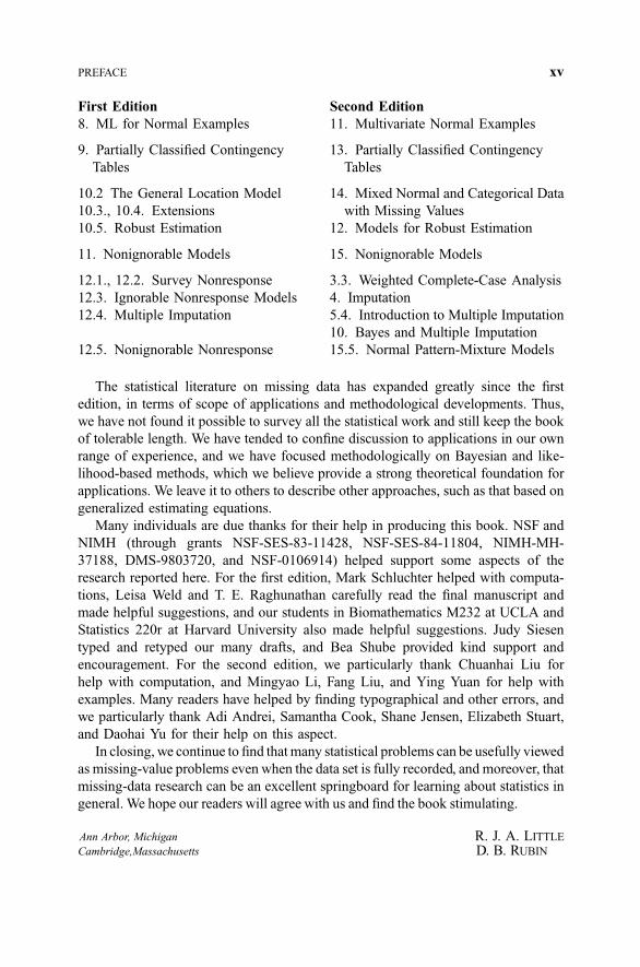
Because the second edition has some major additions and revisions, we provide a

map showing where to locate the material originally appearing in Edition 1.

First Edition

1. Introduction

2. Missing Data in Experiments

3.2. Complete-Case Analysis

3.3. Available-Case Analysis

3.4. Filling in the Missing Values

4.2., 4.3. Randomization Inference with

and without Missing Data

4.4. Weighting Methods

4.5. Imputation Procedures

4.6. Estimation of Sampling Variance

with Nonresponse

5. Theory of Inference Based on the

Likelihood Function

6. Factored Likelihood Methods

7. Maximum Likelihood for General

Patterns of Missing Data

Second Edition

1. Introduction

2. Missing Data in Experiments

3.2. Complete-Case Analysis

3.4. Available-Case Analysis

4.2. Imputing Means from a Predictive

Distribution

Omitted

3.3. Weighted Complete-Case Analysis

4. Imputation

5. Estimation of Imputation Uncertainty

6. Theory of Inference Based on the

Likelihood Function

7. Factored Likelihood Methods,

Ignoring the Missing-Data

Mechanism

8. Maximum Likelihood for General

Patterns

9.1. Standard Errors Based on the

Information Matrix.

xiv PREFACE

The statistical literature on missing data has expanded greatly since the first

edition, in terms of scope of applications and methodological developments. Thus,

we have not found it possible to survey all the statistical work and still keep the book

of tolerable length. We have tended to confine discussion to applications in our own

range of experience, and we have focused methodologically on Bayesian and like-

lihood-based methods, which we believe provide a strong theoretical foundation for

applications. We leave it to others to describe other approaches, such as that based on

generalized estimating equations.

Many individuals are due thanks for their help in producing this book. NSF and

NIMH (through grants NSF-SES-83-11428, NSF-SES-84-11804, NIMH-MH-

37188, DMS-9803720, and NSF-0106914) helped support some aspects of the

research reported here. For the first edition, Mark Schluchter helped with computa-

tions, Leisa Weld and T. E. Raghunathan carefully read the final manuscript and

made helpful suggestions, and our students in Biomathematics M232 at UCLA and

Statistics 220r at Harvard University also made helpful suggestions. Judy Siesen

typed and retyped our many drafts, and Bea Shube provided kind support and

encouragement. For the second edition, we particularly thank Chuanhai Liu for

help with computation, and Mingyao Li, Fang Liu, and Ying Yuan for help with

examples. Many readers have helped by finding typographical and other errors, and

we particularly thank Adi Andrei, Samantha Cook, Shane Jensen, Elizabeth Stuart,

and Daohai Yu for their help on this aspect.

In closing, we continue to find that many statistical problems can be usefully viewed

as missing-value problems even when the data set is fully recorded, and moreover, that

missing-data research can be an excellent springboard for learning about statistics in

general. We hope our readers will agree with us and find the book stimulating.

Ann Arbor, Michigan R. J. A. LITTLE

Cambridge,Massachusetts D. B. RUBIN

First Edition

8. ML for Normal Examples

9. Partially Classified Contingency

Tables

10.2 The General Location Model

10.3., 10.4. Extensions

10.5. Robust Estimation

11. Nonignorable Models

12.1., 12.2. Survey Nonresponse

12.3. Ignorable Nonresponse Models

12.4. Multiple Imputation

12.5. Nonignorable Nonresponse

Second Edition

11. Multivariate Normal Examples

13. Partially Classified Contingency

Tables

14. Mixed Normal and Categorical Data

with Missing Values

12. Models for Robust Estimation

15. Nonignorable Models

3.3. Weighted Complete-Case Analysis

4. Imputation

5.4. Introduction to Multiple Imputation

10. Bayes and Multiple Imputation

15.5. Normal Pattern-Mixture Models

PREFACE xv


Second Edition

P A R T I

Overview and BasicApproaches

C H A P T E R 1

Introduction

1.1. THE PROBLEM OF MISSING DATA

Standard statistical methods have been developed to analyze rectangular data sets.

Traditionally, the rows of the data matrix represent units, also called cases, observa-

tions, or subjects depending on context, and the columns represent variables

measured for each unit. The entries in the data matrix are nearly always real

numbers, either representing the values of essentially continuous variables, such

as age and income, or representing categories of response, which may be ordered

(e.g., level of education) or unordered (e.g., race, sex). This book concerns the

analysis of such a data matrix when some of the entries in the matrix are not

observed. For example, respondents in a household survey may refuse to report

income. In an industrial experiment some results are missing because of mechanical

breakdowns unrelated to the experimental process. In an opinion survey some indi-

viduals may be unable to express a preference for one candidate over another. In the

first two examples it is natural to treat the values that are not observed as missing, in

the sense that there are actual underlying values that would have been observed if

survey techniques had been better or the industrial equipment had been better

maintained. In the third example, however, it is less clear that a well-defined candi-

date preference has been masked by the nonresponse; thus it is less natural to treat

the unobserved values as missing. Instead the lack of a response is essentially an

additional point in the sample space of the variable being measured, which identifies

a ‘‘no preference’’ or ‘‘don’t know’’ stratum of the population.

Most statistical software packages allow the identification of nonrespondents by

creating one or more special codes for those entries of the data matrix that are not

observed. More than one code might be used to identify particular types of non-

response, such as ‘‘don’t know,’’ or ‘‘refuse to answer,’’ or ‘‘out of legitimate range.’’

Some statistical packages typically exclude units that have missing value codes for

any of the variables involved in an analysis. This strategy, which we term a

‘‘complete-case analysis,’’ is generally inappropriate, since the investigator is usually

interested in making inferences about the entire target population, rather than the

3

portion of the target population that would provide responses on all relevant vari-

ables in the analysis. Our aim is to describe a collection of techniques that are more

generally appropriate than complete-case analysis when missing entries in the data

set mask underlying values.

1.2. MISSING-DATA PATTERNS

We find it useful to distinguish the missing-data pattern, which describes which

values are observed in the data matrix and which values are missing, and the miss-

ing-data mechanism (or mechanisms), which concerns the relationship between

missingness and the values of variables in the data matrix. Some methods of analy-

sis, such as those described in Chapter 7, are intended for particular patterns of

missing data and use only standard complete-data analyses. Other methods, such as

those described in Chapters 8–10, are applicable to more general missing-data

patterns, but usually involve more computing than methods designed for special

patterns. Thus it is beneficial to sort rows and columns of the data according to

the pattern of missing data to see if an orderly pattern emerges. In this section we

discuss some important patterns, and in the next section we formalize the idea of

missing-data mechanisms.

Let Y ¼ ðyijÞ denote an ðn � KÞ rectangular data set without missing values, with

ith row yi ¼ ðyi1; . . . ; yiK Þ where yij is the value of variable Yj for subject i. With

missing data, define the missing-data indicator matrix M ¼ ðmijÞ, such that mij ¼ 1

if yij is missing and mij ¼ 0 if yij is present. The matrix M then defines the pattern of

missing data. Figure 1.1 shows some examples of missing-data patterns. Some

methods for handling missing data apply to any pattern of missing data, whereas

other methods are restricted to a special pattern.

EXAMPLE 1.1. Univariate Missing Data. Figure 1.1a illustrates univariate missing

data, where missingness is confined to a single variable. The first incomplete-data

problem to receive systematic attention in the statistics literature has the pattern of

Figure 1.1a, namely, the problem of missing data in designed experiments. In the

context of agricultural trials this situation is often called the missing-plot problem.

Interest is in the relationship between a dependent variable YK , such as yield of crop,

on a set of factors Y1; . . . ; YK�1, such as variety, type of fertilizer, and temperature,

all of which are intended to be fully observed. (In the figure, K ¼ 5.) Often a

balanced experimental design is chosen that yields orthogonal factors and hence a

simple analysis. However, sometimes the outcomes for some of the experimental

units are missing (for example because of lack of germination of a seed, or because

the data were incorrectly recorded). The result is the pattern with YK incomplete and

Y1; . . . ; YK�1 fully observed. Missing-data techniques fill in the missing values of YK

in order to retain the balance in the original experimental design. Historically

important methods, reviewed in Chapter 2, were motivated by computational

simplicity and hence are less important in our era of high-speed computers, but

they can still be useful in high-dimensional problems.

4 INTRODUCTION

EXAMPLE 1.2. Unit and Item Nonresponse in Surveys. Another common pattern is

obtained when the single incomplete variable YK in Figure 1.1a is replaced by a set

of variables YJþ1; . . . ; YK , all observed or missing on the same set of cases (see

Figure 1.1b, where K ¼ 5 and J ¼ 2). An example of this pattern is unit

nonresponse in sample surveys, where a questionnaire is administered and a

subset of sampled individuals do not complete the questionnaire because of

noncontact, refusal, or some other reason. In that case the survey items are the

incomplete variables, and the fully observed variables consist of survey design

variables measured for respondents and nonrespondents, such as household location

or characteristics measured in a listing operation prior to the survey. Common

techniques for addressing unit nonresponse in surveys are discussed in Chapter 3.

Figure 1.1. Examples of missing-data patterns. Rows correspond to observations, columns to variables.

1.2. MISSING-DATA PATTERNS 5

Survey practitioners call missing values on particular items in the questionnaire item

nonresponse. These missing values typically have a haphazard pattern, such as that

in Figure 1.1d. Item nonresponse in surveys is typically handled by imputation

methods as discussed in Chapter 4, although the methods discussed in Part II of the

book are also appropriate and relevant. For other discussions of missing data in the

survey context, see Madow and Olkin (1983), Madow, Nisselson, and Olkin (1983),

Madow, Olkin, and Rubin (1983), Rubin (1987a) and Groves et al. (2002).

EXAMPLE 1.3. Attrition in Longitudinal Studies. Longitudinal studies collect

information on a set of cases repeatedly over time. A common missing-data problem

is attrition, where subjects drop out prior to the end of the study and do not return.

For example, in panel surveys members of the panel may drop out because they

move to a location that is inaccessible to the researchers, or, in a clinical trial, some

subjects drop out of the study for unknown reasons, possibly side effects of drugs, or

curing of disease. The pattern of attrition is an example of monotone missing data,

where the variables can be arranged so that all Yjþ1; . . . ; YK are missing for cases

where Yj is missing, for all J ¼ 1; . . . ;K � 1 (see Figure 1.1c for K ¼ 5). Methods

for handling monotone missing data can be easier than methods for general patterns,

as shown in Chapter 7 and elsewhere.

In practice, the pattern of missing data is rarely monotone, but is often close to

monotone. Consider for example the data pattern in Table 1.1, which was obtained

from the results of a panel study of students in 10 Illinois schools, analyzed by

Marini, Olsen, and Rubin (1980). The first block of variables was recorded for all

Table 1.1 Patterns of Missing Data across Four Blocks of Variables: 0 ¼ observed,

1 ¼ missing).

Variables

Variables Measured

Measured Only for

for All Initial

Adolescent Follow-Up Follow-Up Parent Number

Variables, Respondents, Respondents, Variables, of Percentage

Pattern Block 1 Block 2 Block 3 Block 4 Cases of Cases

A 0 0 0 0 1594 36.6

B 0 0a 0a 1 648 14.9

C 0 0 1 0b 722 16.6

D 0 0a 1 1 469 10.8

E 0 1 1 0b 499 11.5

F 0 1 1 1 420 9.6

Total 4352 100:0

Source: Marini, Olsen, and Rubin 1980.aObservations falling outside monotone pattern 2 (block 1 more observed than block 4; block 4 more

observed than block 2; block 2 more observed than block 3).bObservations falling outside monotone pattern 1 (block 1 more observed than block 2; block 2 more

observed than block 3; block 3 more observed than block 4).

6 INTRODUCTION

individuals at the start of the study, and hence is completely observed. The second

block consists of variables measured for all respondents in the follow-up study, 15

years later. Of all respondents to the original survey, 79% responded to the follow-

up, and thus the subset of variables in block 2 is regarded as 79% observed. Block 1

variables are consequently more observed than block 2 variables. The data for the

15-year follow-up survey were collected in several phases, and for economic reasons

the group of variables forming the third block were recorded for a subset of those

responding to block 2 variables. Thus, block 2 variables are more observed than

block 3 variables. Blocks 1, 2, and 3 form a monotone pattern of missing data. The

fourth block of variables consists of a small number of items measured by a ques-

tionnaire mailed to the parents of all students in the original adolescent sample. Of

these parents, 65% responded. The four blocks of variables do not form a monotone

pattern. However, by sacrificing a relatively small amount of data, monotone patterns

can be obtained. The authors analyzed two monotone data sets. First, the values of

block 4 variables for patterns C and E (marked with the letter b) are omitted, leaving

a monotone pattern with block 1 more observed than block 2, which is more

observed than block 3, which is more observed than block 4. Second, the values

of block 2 variables for patterns B and D and the values of block 3 variables for

pattern B (marked with the letter a) are omitted, leaving a monotone pattern with

block 1 more observed than block 4, which is more observed than block 2, which is

more observed than block 3. In other examples (such as the data in Table 1.2,

discussed in Example 1.6 below), the creation of a monotone pattern involves the

loss of a substantial amount of information.

EXAMPLE 1.4. The File-Matching Problem, with Two Sets of Variables Never

Jointly Observed. With large amounts of missing data, the possibility that variables

are never observed together arises. When this happens, it is important to be aware of

the problem since it implies that some parameters relating to the association between

these variables are not estimable from the data, and attempts to estimate them may

yield misleading results. Figure 1.1e illustrates an extreme version of this problem

that arises in the context of combining data from two sources. In this pattern, Y1

Table 1.2 Data Matrix for Children in a Survey Summarized by the Pattern of Missing

Data: 0 ¼ observed, 1 ¼ missing.

Variables

N of Children

Pattern Age Gender Weight 1 Weight 2 Weight 3 with Pattern

A 0 0 0 0 0 1770

B 0 0 0 0 1 631

C 0 0 0 1 0 184

D 0 0 1 0 0 645

E 0 0 0 1 1 756

F 0 0 1 0 1 370

G 0 0 1 1 0 500


represents a set of variables that is common to both data sources and fully-observed,

Y2 a set of variables observed for the first data source but not the second, and Y3 a set

of variables observed for the second data source but not the first. Clearly there is no

information in this data pattern about the partial associations of Y2 and Y3 given Y1;

in practice, analyses of data with this pattern typically make the strong assumption

that these partial associations are zero. This pattern is discussed further in Section

7.5.

EXAMPLE 1.5. Latent-Variable Patterns with Variables that are Never Observed. It

can be useful to regard certain problems involving unobserved ‘‘latent’’ variables as

missing-data problems where the latent variables are completely missing, and then

apply ideas from missing-data theory to estimate the parameters. Consider, for

example, Figure 1.1f , where X represents a set of latent variables that are completely

missing, and Y a set of variables that are fully observed. Factor analysis can be

viewed as an analysis of the multivariate regression of Y on X for this pattern—that

is, a pattern with none of the regressor variables observed! Clearly, some assump-

tions are needed. Standard forms of factor analysis assume the conditional inde-

pendence of the components of Y given X . Estimation can be achieved by treating

the factors X as missing data. If values of Y are also missing according to a

haphazard pattern, then methods of estimation can be developed that treat both X

and the missing values of Y as missing. This example is examined in more detail in

Section 11.3.

We make the following key assumption throughout the book:

Assumption 1.1: missingness indicators hide true values that are meaningful

for analysis.

Assumption 1.1 may seem innocuous, but it has important implications for the

analysis. When the assumption applies, it makes sense to consider analyses that

effectively predict, or ‘‘impute’’ (that is, fill in) the unobserved values. If, on the

other hand, Assumption 1.1 does not apply, then imputing the unobserved values

makes little sense, and an analysis that creates strata of the population defined by the

missingness indicator is more appropriate. Example 1.6 describes a situation with

longitudinal data on obesity where Assumption 1.1 clearly makes sense. Example

1.7 describes the case of a randomized experiment where it makes sense for one

outcome variable (survival) but not for another (quality of life). Example 1.8

describes a situation in opinion polling where Assumption 1.1 may or may not

make sense, depending on the specific setting.

EXAMPLE 1.6. Nonresponse in a Binary Outcome Measured at Three Time

Points. Woolson and Clarke (1984) analyze data from the Muscatine Coronary

Risk Factor Study, a longitudinal study of coronary risk factors in schoolchildren.

Table 1.2 summarizes the data matrix by its pattern of missing data. Five variables

(gender, age, and obesity for three rounds of the survey) are recorded for 4856

cases—gender and age are completely recorded, but the three obesity variables are

sometimes missing with six patterns of missingness. Since age is recorded in five

8 INTRODUCTION

categories and the obesity variables are binary, the data can be displayed as counts in

a contingency table. Table 1.3 displays the data in this form, with missingness of

obesity treated as a third category of the variable, where O ¼ obese, N ¼ not obese,

and M ¼ missing. Thus the pattern MON denotes missing at the first round, obese at

the second round, and not obese at the third round, and other patterns are defined

similarly.

Woolson and Clarke analyze these data by fitting multinomial distributions over

the 33 � 1 ¼ 26 response categories for each column in Table 1.3. That is, missing-

ness is regarded as defining strata of the population. We suspect that for these data it

Table 1.3 Number of Children Classified by Population and Relative Weight Category

in Three Rounds of a Survey

Males Females

Age Group Age Group

Response

Categorya 5–7 7–9 9–11 11–13 13–15 5–7 7–9 9–11 11–13 13–15

NNN 90 150 152 119 101 75 154 148 129 91

NNO 9 15 11 7 4 8 14 6 8 9

NON 3 8 8 8 2 2 13 10 7 5

NOO 7 8 10 3 7 4 19 8 9 3

ONN 0 8 7 13 8 2 2 12 6 6

ONO 1 9 7 4 0 2 6 0 2 0

OON 1 7 9 11 6 1 6 8 7 6

OOO 8 20 25 16 15 8 21 27 14 15

NNM 16 38 48 42 82 20 25 36 36 83

NOM 5 3 6 4 9 0 3 0 9 15

ONM 0 1 2 4 8 0 1 7 4 6

OOM 0 11 14 13 12 4 It 17 13 23

NMN 9 16 13 14 6 7 16 8 31 5

NMO 3 6 5 2 1 2 3 1 4 0

OMN 0 1 0 1 0 0 0 1 2 0

OMO 0 3 3 4 1 1 4 4 6 1

MNN 129 42 36 18 13 109 47 39 19 11

MNO 18 2 5 3 1 22 4 6 1 1

MON 6 3 4 3 2 7 1 7 2 2

MOO 13 13 3 1 2 24 8 13 2 3

NMM 32 45 59 82 95 23 47 53 58 89

OMM 5 7 17 24 23 5 7 16 37 32

MNM 33 33 31 23 34 27 23 25 21 43

MOM 11 4 9 6 12 5 5 9 1 15

MMN 70 55 40 37 15 65 39 23 23 14

MMO 24 14 9 14 3 19 13 8 10 5

Source: Woolson and Clarke (1984).aNNN indicates not obese in 1977, 1979, and 1981; O indicates obese, and M indicates missing in a given

year.


makes good sense to regard the nonrespondents as having a true underlying value for

the obesity variable. Hence we would argue for treating the nonresponse categories

as missing value indicators and estimating the joint distribution of the three dichot-

omous outcome variables from the partially missing data. Appropriate methods

for handling such categorical data with missing values effectively impute the

values of obesity that are not observed, and are described in Chapter 12. The

methods involve quite straightforward modifications of existing algorithms for cate-

gorical data analysis currently available in statistical software packages. For an

analysis of these data that averages over patterns of missing data, see Ekholm and

Skinner (1998).

EXAMPLE 1.7. Causal Effects of Treatments with Survival and Quality of Life

Outcomes. Consider a randomized experiment with two drug treatment conditions,

T ¼ 0 or 1, and suppose that a primary outcome of the study is survival (D ¼ 0) or

death (D ¼ 1) at one year after randomization to treatment. For participant i, let

Dið0Þ denote the one-year survival status if assigned treatment 0, and Dið1Þ survival

status if assigned treatment 1. The causal effect of treatment 1 relative to treatment 0

on survival for participant i is defined as Dið1Þ � Dið0Þ. Estimation of this causal

effect can be considered a missing-data problem, in that only one treatment can be

assigned to each participant, so Dið1Þ is unobserved (‘‘missing’’) for participants

assigned treatment 0, and Dið1Þ is unobserved (‘‘missing’’) for participants assigned

treatment 1. Individual causal effects are unobserved, but randomization allows for

unbiased estimation of average causal effects for a sample or population (Rubin,

1978a), which can be estimated from this missing-data perspective. The survival

outcome under the treatment not received can be legitimately modeled as ‘‘missing

data’’ in the sense of Assumption 1.1, since one can consider what the survival

outcome would have been under the treatment not assigned, even though this

outcome is never observed. For more applications of this ‘‘potential outcome’’

formulation to inference about causal effects, see, for example, Angrist, Imbens, and

Rubin (1996), Barnard et al. (1998), Hirano et al. (2000), and Frangakis and Rubin

(1999, 2001, 2002).

Rubin (2000) discusses the more complex situation where a ‘‘quality-of-life

health indicator’’ Y ðY > 0Þ is also measured as a secondary outcome for those

still alive one year after randomization to treatment. For participants who die

within a year of randomization, Y is undefined in some sense or ‘‘censored’’ due

to death—we think it usually makes little sense to treat these outcomes as missing

values as in Assumption 1.1, given that quality of life is a meaningless concept for

people who are not alive. More specifically, let DiðT Þ denote the potential one-year

survival outcome for participant i under treatment T , as before. The potential

outcomes on D can be used to classify the patients into four groups:

1. Those who would live under either treatment assignment, LL ¼

fijDið0Þ ¼ Dið1Þ ¼ 0g

2. Those who would die under either treatment assignment, DD ¼

fijDið0Þ ¼ Dið1Þ ¼ 1g

10 INTRODUCTION

statistical analysis with missing...

Documents