statistical analysis of vehicletimeheadways -...
TRANSCRIPT
Teknillinen korkeakouluLiikennetekniikkaJulkaisu 87
Statistical Analysis ofVEHICLE TIME HEADWAYS
R. Tapio LuttinenTL Consulting Engineers, Ltd.
Dissertation for the degree of Doctor of Technology to be presented with duepermission for public examination and debate in the Auditorium at the HelsinkiUniversity of Technology Lahti Center (Neopoli, Lahti, Finland) on the 31st ofMay, 1996, at 12 o’clock noon.
Otaniemi 1996

Julkaisu—Publication:
Luttinen, R. Tapio, Statistical Analysis of Vehicle Time Headways.Teknillinen korkeakoulu, Liikennetekniikka, Julkaisu 87. Otaniemi, 1996.
Luttinen, R. Tapio, Statistical Analysis of Vehicle Time Headways.Helsinki University of Technology, Transportation Engineering, Publication87. Otaniemi, 1996.
This book was prepared with LATEX and reproduced from a Postscript filesupplied by the author.
Copyright c© 1996 by R. Tapio LuttinenSecond corrected printing
ISBN 951-22-3063-1ISSN 0781-5816
Printed in Finland by Gummerus Printing, Saarijarvi, 1996

To Tarja, Mikko, Hanna, and Jaakko
For want of skilful strategy an army is lost;victory is the fruit of long planning.
Proverbs 11:14 (The New English Bible)


Luttinen, R. Tapio, Statistical Analysis of Vehicle Time Headways. Teknillinenkorkeakoulu, Liikennetekniikka, Julkaisu 87. Otaniemi, 1996. ISBN 951-22-3063-1.ISSN 0781-5816. UDC 656.021.
Keywords: traffic flow, headways, capacity, level of service, statistics, param-eter estimation, goodness of fit, moving probability, Monte Carlo method
Abstract
The properties of vehicle time headways are fundamental in many trafficengineering applications, such as capacity and level of service studies onhighways, unsignalized intersections, and roundabouts. The operation ofmodern vehicle-actuated traffic signals is based on the measurement of timeheadways in the arriving traffic flow. In addition, the vehicle generationin traffic flow simulation is usually based on some theoretical vehicle timeheadway model.
The statistical analysis of vehicle time headways has been inadequatein three important aspects: 1) There has been no standard procedure tocollect headway data and to describe their statistical properties. 2) Thegoodness-of-fit tests have been either powerless or infeasible. 3) Test resultsfrom multi-sample data have not been combined properly.
A four-stage identification process is suggested to describe the headwaydata and to compare it with theoretical distributions. The process includesthe estimation of the probability density function, the hazard function, thecoefficient of variation, and the squared skewness and the kurtosis. Thefour-stage identification process effectively describes those properties of thedistribution that are most helpful in selecting a theoretical headway model.
One of the major problems in the headway studies has been the methodfor goodness-of-fit tests. The two most commonly used tests are the chi-square test and the nonparametric Kolmogorov-Smirnov test. The chi-square test is not very powerful. The nonparametric Kolmogorov-Smirnovtest should be applied only, when the parameters of the distribution areknown. If the parameters are estimated from the data, as in typical headwaystudies, the nonparametric Kolmogorov-Smirnov test gives too conservativeresults. These problems are addressed by parametric goodness-of-fit testsbased on Monte Carlo methods.
Another great problem has been the lack of theoretical foundation indealing with multi-sample data. The headway data usually consist of severalsamples, and the null hypothesis is tested against each of them. Two meth-ods are presented to strengthen the evidence of multi-sample tests: 1) Thecombined probability method gives a single significance probability based

on several independent tests. 2) The moving probability method is used todescribe the variation of combined probabilities against traffic volume.
These methods were applied to time headway data from Finnish two-lane two-way roads. The independence of consecutive headways was testedusing autocorrelation analysis, runs tests and goodness-of-fit tests for thegeometric bunch size distribution. The results indicate that the renewalhypothesis should not be accepted in all traffic situations. This conclusionis partly supported by a further analysis of previous studies.
Five theoretical distributions were tested for goodness of fit: the negativeexponential distribution, the shifted exponential distribution, the gammadistribution, the lognormal distribution and the semi-Poisson distribution.None of these passed the tests. In the parameter estimation the maximumlikelihood method was preferred. For distributions having a location (thresh-old) parameter, a modified maximum likelihood method was shown to givegood estimates.
The proposed procedures give a scientific foundation to identify and esti-mate statistical models for vehicle time headways, and to test the goodnessof fit. It is shown that the statistical methods in the analysis of vehicleheadways should be thoroughly revised following the guidelines presentedhere.

Contents
Glossary of Notation 9
Preface 13
1 Introduction 151.1 Definitions . . . . . . . . . . . . . . . . . . . . . . . . . . . . . 151.2 Importance of headway studies . . . . . . . . . . . . . . . . . 161.3 History and problems . . . . . . . . . . . . . . . . . . . . . . 161.4 Purpose of the study . . . . . . . . . . . . . . . . . . . . . . . 191.5 Summary of contents . . . . . . . . . . . . . . . . . . . . . . . 19
2 Theoretical background 212.1 Microscopic traffic flow theory . . . . . . . . . . . . . . . . . . 212.2 Statistical methods . . . . . . . . . . . . . . . . . . . . . . . . 26
2.2.1 Sampling techniques . . . . . . . . . . . . . . . . . . . 262.2.2 Trend tests . . . . . . . . . . . . . . . . . . . . . . . . 292.2.3 Parameter estimation . . . . . . . . . . . . . . . . . . 322.2.4 Goodness-of-fit tests . . . . . . . . . . . . . . . . . . . 352.2.5 Combination of probabilities . . . . . . . . . . . . . . 432.2.6 Moving probability . . . . . . . . . . . . . . . . . . . . 45
3 Data collection 473.1 Measurements . . . . . . . . . . . . . . . . . . . . . . . . . . . 473.2 Preliminary data analysis . . . . . . . . . . . . . . . . . . . . 483.3 Selection of trend free samples . . . . . . . . . . . . . . . . . 493.4 Description of selected samples . . . . . . . . . . . . . . . . . 49
4 Identification 534.1 The purpose of identification . . . . . . . . . . . . . . . . . . 534.2 Shape of the distribution . . . . . . . . . . . . . . . . . . . . . 54
7

8 CONTENTS
4.2.1 Empirical distribution function . . . . . . . . . . . . . 544.2.2 Empirical density function . . . . . . . . . . . . . . . . 574.2.3 Empirical hazard function . . . . . . . . . . . . . . . . 60
4.3 Measures of location and dispersion . . . . . . . . . . . . . . . 644.3.1 Mode and peak height . . . . . . . . . . . . . . . . . . 644.3.2 Median . . . . . . . . . . . . . . . . . . . . . . . . . . 664.3.3 Coefficient of variation . . . . . . . . . . . . . . . . . . 684.3.4 Skewness and kurtosis . . . . . . . . . . . . . . . . . . 72
4.4 Tests for the renewal hypothesis . . . . . . . . . . . . . . . . . 744.4.1 Background . . . . . . . . . . . . . . . . . . . . . . . . 744.4.2 Autocorrelation . . . . . . . . . . . . . . . . . . . . . . 754.4.3 Randomness . . . . . . . . . . . . . . . . . . . . . . . 804.4.4 Platoon length . . . . . . . . . . . . . . . . . . . . . . 82
4.5 Discussion . . . . . . . . . . . . . . . . . . . . . . . . . . . . . 84
5 Theoretical headway models 875.1 Principles of evaluation . . . . . . . . . . . . . . . . . . . . . 875.2 Simple Distributions . . . . . . . . . . . . . . . . . . . . . . . 88
5.2.1 Negative exponential distribution . . . . . . . . . . . . 885.2.2 Shifted exponential distribution . . . . . . . . . . . . . 945.2.3 Gamma distribution . . . . . . . . . . . . . . . . . . . 1015.2.4 Lognormal distribution . . . . . . . . . . . . . . . . . 117
5.3 Mixed distributions . . . . . . . . . . . . . . . . . . . . . . . . 1275.3.1 Structure of the model . . . . . . . . . . . . . . . . . . 1275.3.2 Properties of the model . . . . . . . . . . . . . . . . . 1295.3.3 The exponential tail hypothesis . . . . . . . . . . . . . 1305.3.4 Hyperexponential distribution . . . . . . . . . . . . . . 1395.3.5 Hyperlang distribution . . . . . . . . . . . . . . . . . . 1435.3.6 M/D/1 queuing model . . . . . . . . . . . . . . . . . . 1465.3.7 Generalized queuing model . . . . . . . . . . . . . . . 1495.3.8 Semi-Poisson distribution . . . . . . . . . . . . . . . . 155
6 Conclusions and recommendations 173
References 179
A Data description 191

Glossary of Notation
A2 Anderson-Darling statisticA-D Anderson-DarlingANCOVA Analysis of covarianceBAN Best asymptotically normalBLUE Best linear unbiased estimatorC Sample coefficient of variationC(T ) Coefficient of variation of the distribution for Tcorr(x,y) Correlation coefficient between x and yc.v. Coefficient of variationD Deterministic distributionD Kolmogorov-Smirnov statisticE(T ) Expectation for random variable TEDF Empirical distribution functionedf Empirical density functionehf Empirical hazard functioneq. Equationexp(x) Exponential function (ex)F(t) Probability distribution function (P{T ≤ t})Fn(t) Empirical probability distribution function for sample of
size nf(t) Probability density functionf∗(s) Laplace transform of f(t)fig. FigureG General distributionHCM Highway Capacity Manualh(t) Hazard functioni.i.d. Independent and identically distributedK(x) Kernel functionK-S Kolmogorov-SmirnovM Exponential distribution
9

10 GLOSSARY OF NOTATION
M’ Modified exponential distributionm Number of replications, number of samplesmk The kth central sample moment
∑nj=1(xj − x)k/n
m′k The kth noncentral sample moment
∑nj=1 xk
j /n
MCS Minimum chi-squareMd MedianMLE Maximum likelihood estimatorMME Method of moments estimatorMMLE Modified maximum likelihood estimatorMMME Modified method of moments estimatorMo ModeMVUE Minimum variance unbiased estimatorsN(t) Number of events in (0, t]N(a,b] Number of events in (a, b]N(µ,σ) Normal distribution with mean µ and standard deviation σn Sample sizeo(∆) lim∆→0 o(∆)/∆ = 0P Significance probability (P-value of a test), combined
probabilityPk(λk,j) The jth term of a k-point moving probabilityp Probability, proportion of follower headwayspi Significance probability (P-value of a test) for sample iP(A-D) Significance probability of the Anderson-Darling testP(K-S) Significance probability of the Kolmogorov-Smirnov testPDF Probability distribution functionpdf Probability density functionPh Peak heightP{A} Probability of event AQ Kendall’s rank correlation test statisticRe = Re1 Set of real numbersRe+ Set of positive real numbersR2 Coefficient of determination (multiple correlation coefficient)r Pearson’s correlation coefficientrxy Sample correlation coefficient between x and yrxy·z Sample correlation coefficient between x and y with z
held constantr.v. Random variablerrmse Relative root mean square errorS Weighted sign test statistic

11
s Sample standard deviation, Laplace transform variableSr Sum of r random variatess.e. Standard errorSL Speed limit [km/h]T Time headway variablet Time headway (value)t Sample mean of headwaysti The ith headwayT(1) The first order statistic of the distribution for T
t(1) The first order statistic of a sample; i.e., min{t1, . . . ,tn}U(a,b) Uniform (rectangular) distribution between a and bV Exponential ordered scores test statisticW 2 Cramer-von Mises statisticX+ Positive part of X; i.e., (X + |X|)/2xj(ω) Position of vehicle j at time ωxj(ω) Differential of xj with respect to ω (speed)xj(ω) Second differential of xj with respect to ω (acceleration)α Shape parameter of the gamma distributionα3(T ) Skewness of the distribution for Tα3 Sample skewnessα4(T ) Kurtosis of the distribution for Tα4 Sample kurtosisβ Scale parameter of the gamma distributionΓ(x) Gamma functionγ(a,x) Incomplete gamma functionδ Threshold for exponential tailθ Parameter of a distributionθ Maximum likelihood estimator for θ
θ Modified maximum likelihood estimator for θ
θ Minimum chi-square estimator for θ
θ Estimator for θλ Flow rate, traffic intensityλ Traffic volume, estimated flow rateµ Scale parameter of the lognormal distributionµ(T ) Mean of the distribution for Tν Degrees of freedomρ Server utilization factorρi Autocorrelation coefficient at lag iρi Sample autocorrelation coefficient at lag i
12 GLOSSARY OF NOTATION
ρi·x Partial correlation coefficient for autocorrelation at lag iwith x held constant
σ Shape parameter of the lognormal distribution,σ(T ) Standard deviation of the distribution for Tσ2(T ) Variance of the distribution for Tτ Location (threshold) parameter of a headway distribution,
rank correlation coefficient (Kendall’s τ)υ Speed differenceΦ(X) Probability distribution function of the standard normal
distributionφ(X) Probability density function of the standard normal
distributionω Time∗ Convolution operator#{ x | A } Number of x’s fulfilling condition A

Preface
The work started with the aim of finding more effective methods for vehicle-actuated traffic signal control on two-lane roads. Part of the project wasthe development of a traffic signal control simulation program. In order tofind a suitable headway variate generator, some field measurements wereperformed on two-lane roads with speed limits not greater than 70 km/h.(In Finland traffic signal control is not allowed on roads with higher speedlimits.) The location and time of each measurement was selected so thatthe expected flow rate would not be much above 1,000 veh/h.
The analysis of the vehicle time headway data soon appeared to be afar more complex issue than was initially assumed. It became evident thatthe methods commonly used in the literature were not very efficient, andin many cases they were infeasible. Consequently, the focus of the studyshifted from traffic signal control to the statistical analysis of vehicle head-ways. Some shortcomings in this report are due to this fact. When thefield measurements were made, the extent and type of the analyses to beperformed was not anticipated.
Many of the theoretical distributions and their basic properties have beendescribed in an introductory paper (Luttinen 1990). The major results havebeen published earlier: the goodness-of-fit tests and parameter estimationfor the gamma distribution (Luttinen 1991); the basic statistical propertiesof time headways (Luttinen 1992); and the methods of identification, es-timation, and goodness-of-fit tests (Luttinen 1994). The comments of thereviewers of these papers have been very helpful.
The traffic analyzer measurements were performed by the Laboratory ofTransportation Engineering at the Helsinki University of Technology. Myspecial thanks to Mr. Kari Hintikka for all the care he has taken with themeasurements. I gratefully acknowledge professors Arde Faghri, Sulevi Lyly,Hannu Niemi and Matti Pursula for their advice and support. ProfessorFaghri has given very valuable help to make the purpose and style of thetext more clear. Professor Lyly has helped me in many practical matters.
13

14 PREFACE
Professor Niemi’s detailed comments on statistical and mathematical aspectshave been extremely helpful. Professor Pursula’s expertise in traffic flowtheory has saved me from many pitfalls.
Many of the analyses would have been impossible to carry out withoutthe financial support from the Henry Ford Foundation in Finland.
Finally, my deepest thanks to my wife Tarja, to my children Mikko,Hanna, and Jaakko, and to my parents Raili and Matti for their continuoussupport during the past years. Without their patience and encouragementthis report would never have seen the daylight.
Lahti, FinlandApril 28, 1996
R. Tapio Luttinen

Chapter 1
Introduction
1.1 Definitions
Time headway, or headway for short, is the time interval between two vehi-cles passing a point as measured from the front bumper to the front bumper.A headway is accordingly the sum of the time used by a vehicle to pass theobservation point (occupancy time) and the time interval (gap) to the arrivalof the next vehicle.
In platoons the gap is usually more meaningful to the driver than theheadway. Headways are, however, more important in the traffic flow theory.Because the flow rate1 is reciprocal to the mean headway, the study ofheadways is closely connected to the study of highway capacity. In selectinga headway a driver establishes a flow rate for the vehicle (Dawson & Chimini1968).
The headways are measured in time rather than in space. Time head-ways, rather than space headways or spacings between consecutive vehicles,have been selected as the subject because:
1. Time headways and flow rates are directly connected. There is a simi-lar connection between spacings and densities, but flow rates are usu-ally more meaningful and more easily measured by practicing trafficengineers.
2. In platoons the driver of a trailing vehicle adjusts the gap consideringsafety, one aspect of which is the reaction time. It can be assumed
1The flow rate or traffic flow means the expected number of vehicles per time unitpassing the reference point. The traffic volume is the measured number of vehicles pertime unit. In HCM (1994) the terms have been used in a different sense.
15

16 CHAPTER 1. INTRODUCTION
that the gap, and hence the headway of a trailing vehicle, is not assensitive to vehicle speeds as the spacing.
3. An estimate of the spacing can be obtained as the product of speedand headway, assuming constant speed during the headway.
In the literature on point processes the counting specification is oftentaken as primary, because it allows a generalization to higher dimensionalspaces (e.g., Daley & Vere-Jones 1988). This study, however, discusses thetraffic flow as a process on the real line. For this purpose the intervalspecification is more informative.
1.2 Importance of headway studies
Many traffic operations (such as passing, merging, and crossing) dependon the availability of large headways in the traffic flow. Consequently, thedistribution of headways has an effect on platoon formation and delays.
In the 1985 Highway Capacity Manual (HCM 1985) the level of serviceon two-lane rural highways is approximated by the proportion of headwaysless than five seconds—thus making a connection between the headway dis-tribution and the level of service. In addition, the headways play a crucialrole in the analysis of unsignalized intersections and roundabouts (Sullivan& Troutbeck 1994).
Although the average delay in fixed time traffic signals is not very sensi-tive to the detailed stochastic properties of the arrival model (Newell 1956,Newell 1965, Kingman 1962), in vehicle actuated traffic signals the con-trol, the extension time in particular, is very sensitive to the arrival pattern(Darroch, Newell & Morris 1964). The characteristics of vehicle headwaysare accordingly quite relevant in the study of optimal traffic signal control.
The mathematical analysis and simulation of traffic operations are basedon theoretical models, which must be evaluated against the properties of realworld data. More advanced methods have increased the need for reliableknowledge of the statistical properties of vehicle headways.
1.3 History and problems
Traffic flow has been considered as a stochastic process at least since Adams(1936). He formulated the idea of arrivals as a random (i.e., Poisson) processand verified good agreement with theory and observations. Since then manymore sophisticated models have been proposed.

1.3. History and problems 17
The properties of headways have been extensively studied, especially inthe 60’s. Some of this earlier work is now drawn together and evaluated inthe light of recent data and more powerful statistical methods.
No unified framework has been developed for traffic flow theory. Accord-ingly, the vehicle headway studies have been concentrated on the statisticalanalysis of headway data. There have been, however, some notable excep-tions. Greenberg (1966) has found a connection between the microscopictraffic flow theory and the lognormal follower headway distribution.
An interesting new approach has been developed by Heidemann (1990,1993). He has applied the theory of stochastic processes to analyticallyderive the headway distribution as a function of traffic density. Heidemanncriticizes the statistical approach for lacking in detailed analytical reasonsthat would justify the various types of distributions. His approach mayprovide a link between the macroscopic traffic flow theory and the headwaydistributions, but so far it has not found many applications. The distributionfunction is rather complicated, and its statistical properties have not beenwidely explored. The Heidemann model is not discussed below, but it welldeserves further studies.
The statistical analysis of vehicle headways has been inadequate in threeimportant aspects:
1. There has been no standard procedures to collect headway data andto describe their statistical properties.
2. The goodness-of-fit tests have been either powerless or infeasible.
3. Test results from several samples have not been combined properly.
In the literature on vehicle headways the shape of the empirical (sam-ple) distributions have been mostly described by cumulative distributionfunctions and histograms. In some studies measures such as the mode(May 1961, Summala & Vierimaa 1980, Rajalin & Hassel 1992), the median(May 1961) and the coefficient of variation (May 1965, Buckley 1968, Dunne,Rothery & Potts 1968, Breiman, Lawrence, Goodwin & Bailey 1977, Pur-sula & Sainio 1985, Griffiths & Hunt 1991) have been presented. The re-newal hypothesis (mutually independent and identically distributed head-ways) has also drawn the attention of several researchers (e.g., Dunne et al.1968, Breiman, Gafarian, Lichtenstein & Murthy 1969, Cowan 1975, Chris-sikopoulos, Darzentas & McDowell 1982).

18 CHAPTER 1. INTRODUCTION
The work of Breiman et al. (1969) deserves special attention. They havemade a serious attempt to standardize the analysis of headway data bypresenting a method to determine trendless time periods in the traffic flow,and by introducing a set of three tests for the renewal hypothesis. The ideaof trendless data has not, however, been unanimously accepted. In addition,the comparison of the headway data presented by various authors is difficult,because no standard set of analyses has been applied to identify the mostimportant properties of the headway data.
The goodness of fit has been tested mainly by three methods: (1) graph-ical evaluation, (2) the chi-square test, and (3) the Kolmogorov-Smirnovtest. The graphical evaluation has been based on the probability distribu-tion function (e.g., Akcelik & Chung 1994) or the probability density func-tion (e.g., Buckley 1968). These methods are highly subjective and shouldbe used only in preliminary studies. The use of histograms to estimate theprobability density function has sometimes even produced a distorted ideaof the distribution.2
The chi-square test is theoretically justified, but it is based on the re-duction of observations into counts, which decreases the power of the testconsiderably. The Kolmogorov-Smirnov test has been even more problem-atic. It has been used in its nonparametric form, which is based on theassumption that the parameters of the distribution are known. In the head-way studies the parameters are, however, usually estimated from the data.Because the estimation makes the fit better, the critical values should besmaller. This correction has not been made in any of the studies reviewed.Consequently, the results have been too conservative. The problems asso-ciated with the goodness-of-fit tests have not received proper attention inprevious studies.
Another great problem has been the lack of theoretical foundation indealing with multi-sample data. The headway data usually consist of severalsamples, and the null hypothesis is tested against each sample. The resulthas often been presented as the number or proportion of tests which haveled to the rejection of the null hypothesis (e.g., Buckley 1968, Breiman et al.1969). In some cases even the average significance probability has been used(e.g., Branston 1976). In none of the studies reviewed have the individualtests been properly combined to give a scientifically valid evaluation of theoverall acceptability of the hypothesis.
2The figure on page 459 of Griffiths & Hunt (1991) gives the impression of a bell shapedprobability density function that is not supported by their equation 1.

1.4. Purpose of the study 19
1.4 Purpose of the study
The scope of this study is the statistical analysis of vehicle headways on two-lane two-way roads. The headways on both lanes are analyzed separately.The study has two purposes:
1. To introduce a statistical methodology for the analysis of the headwaydata and for the evaluation of the proposed models
2. To get information about the statistical properties of headways on two-lane two-way roads.
The main objective is to present proper statistical methods for the goodness-of-fit tests and for the combination of significance probabilities. The secondobjective is to present a set of methods to effectively describe the statisticalproperties of headway data. These tests and methods will be applied tosome of the most commonly used headway distribution models. Combinedwith the discussion on the data collection and parameter estimation, thetext presents a scientific foundation for the statistical analysis of vehicleheadways.
Although the data are from two-lane two-way roads, the statistical meth-ods presented can be applied to any headway data. Some methods have evenmore general interest.
1.5 Summary of contents
The presentation follows the statistical modeling process in figure 1.1. Chap-ter 2 reviews the microscopic traffic flow theory in the light of vehicle head-ways. There is also a short introduction to the main statistical methodsused. The problem of combining the test results from several samples issolved by the method of combined probabilities (Fisher 1938). The movingprobability method developed by Luttinen (1992) allows the analysis of testresults over another variable, such as traffic volume.
Chapter 3 discusses the measurements and the preliminary analysis ofthe Finnish headway data. The methods introduced in earlier literature toobtain stationary headway data are evaluated. Because the combination ofsamples introduces a bias in the data, data collection based on trend analysisgives better results.
Chapter 4 introduces methods for model identification. In addition tothe conventional probability distribution function and the probability den-sity function, the shape of the headway distribution is analyzed using the

20 CHAPTER 1. INTRODUCTION
TheoryParameterestimation
GOFtests
Datacollection
Modelidentification
Applications
Figure 1.1: Statistical modeling process
hazard function, which has been extensively applied in life and reliabilitydata analyses. The first four moments are shown to be very informativemeasures of location and dispersion. On the basis of these analyses a four-stage identification process (Luttinen 1994) is introduced. In addition, threemethods are used to test, whether the renewal hypothesis can be acceptedfor the headway data.
Chapter 5 analyses the applicability of several statistical distributions asmodels for the headway distributions on two-lane two-way roads. Main em-phasis is on the goodness-of-fit tests and the parameter3 estimation. Para-metric goodness-of-fit tests are compared with the nonparametric Kolmo-gorov-Smirnov tests.
It is assumed that the reader has a basic knowledge of the probabilitytheory as well as statistical and numerical methods. The theory is describedonly to the extent that is essential to understand the text. More detaileddescriptions can be found in the references given.
3The parameters are called location, scale and shape parameters following the terminol-ogy of D’Agostino & Stephens (1986), Johnson, Kotz & Balakrishnan (1994), and Stuart& Ord (1987). A parameter τ is called the location parameter, if the distribution has the
form f(t− τ), and θ is called the scale parameter, if the form is θf(θt) or1θf
(t
θ
)(Stuart
& Ord 1987). If higher moments (skewness and kurtosis) of a distribution are defined bya third parameter, it is called the shape parameter.

Chapter 2
Theoretical background
2.1 Microscopic traffic flow theory
The microscopic theory of traffic flow describes the movements of vehicleson road sections. The movement of vehicles on a lane can be displayedas a time-space digram (fig. 2.1). The distances between vehicles can bestudied either at a fixed location (headways) or at a fixed time (spacings)or as a dynamic (car-following) model, which is the most comprehensiveapproach. A short review of the car-following models gives a broader viewon the properties of vehicle headways.
Let the position of a vehicle j at a moment ω be xj(ω). The time instantfor the vehicle to pass the observation point (x) is:
ωj(x) = { ω | xj(ω) = x }. (2.1)
Thus, the time headway of vehicle j at point x is:
tj(x) = ωj(x) − ωj−1(x). (2.2)
Assuming constant speed for vehicle j during the headway, the headwayof vehicle j at time ω is:
tj(ω) =xj−1(ω) − xj(ω)
xj(ω), (2.3)
where the numerator is the spacing of vehicle j at time ω, and the dotdenotes differentiation with respect to time. This equation gives the ba-sic relationship between time headways, space headways, and car-followingmodels.
21

22 CHAPTER 2. THEORETICAL BACKGROUND
Position
x
Time
Vehicle j-1
Headway
ω
Spacing
Vehicle j+1Vehicle j
Figure 2.1: Time-space diagram of vehicle trajectories
Let us assume that the driver of vehicle j has reaction time Rj . Thelength of the vehicle ahead is Lj−1. The driver of vehicle j wants to keep anet safety spacing Bj in front of the vehicle. This spacing allows the driverto avoid too strong decelerations. The desired headway is then (Daou 1966):
tj = Rj +Lj−i + Bj
xj−1. (2.4)
Daou analyzed over 24,000 headways from the Holland Tunnel and obtainedleast squares estimates for reaction time Rj = 1.488 s and (gross) safetyspacing Lj−1 + Bj = 35.0 ft (10.7 m).
According to this theory, there is a correlation between desired headwaysand speeds as shown in figure 2.2. At higher speeds the follower headwaysare shorter.
In a car-following model the driver of a following vehicle can control thevehicle by accelerating and decelerating. The researchers in the GeneralMotors (see May 1990) developed several models based on the assumptionthat the response (control) is a function of stimuli and sensitivity.
According to the linear car-following model the response is a linearfunction of the speed difference between the vehicles (Chandler, Herman& Montroll 1958):
xj (ω + Rj) = α0 [xj−1 (ω) − xj (ω)] . (2.5)
Because the response does not depend on the headway or the spacing be-tween vehicles, the model is unrealistic, and it cannot describe the desired

2.1. Microscopic traffic flow theory 23
40 50 60 70 80 90 100
1.8
1.9
2.0
2.1
2.2
2.3
2.4
2.5
Headway [s]
Figure 2.2: Speed and desired headway according to Daou (1966)
headway.Gazis, Herman & Potts (1959) have proposed a nonlinear car-following
model :xj (ω + Rj) =
α1
xj−1 (ω) − xj (ω)[xj−1 (ω) − xj (ω)] , (2.6)
where the sensitivity is a function of a parameter (α1) and the spacing, andthe stimulus is the speed difference between vehicles j − 1 and j.
The model produces different equilibrium headways for different initialheadways and relative speeds. Long initial headways and low initial relativespeeds result in long equilibrium headways.
The headway of a vehicle approaching the vehicle ahead is shown in figure2.3. The leading vehicle has constant speed of 80 km/h. The follower startsthe car-following at initial headway 10 s and speed 100 km/h. Reactiontime is 1.5 seconds. Sensitivity coefficients (α1) are 3.0 m/s (upper curve),2.6 m/s (middle curve), and 2.0 m/s (lower curve). The straight line showsthe headway if the follower maintains constant speed (100 km/h).
Gazis, Herman & Rothery (1961) have further modified the nonlinearmodel:
xj (ω + Rj) = α2xm
j (ω + Rj)
[xj−1 (ω) − xj (ω)]l[xj−1 (ω) − xj (ω)] . (2.7)
Increasing l makes the model less sensitive to the initial headway, becausethe response is more strongly inversely proportional to the spacing. The

24 CHAPTER 2. THEORETICAL BACKGROUND
0 20 40 60 80 1000
1
2
3
4
5
6
7
8
9
10Headway [s]
2.6
2.0Constant speed
3.0
Leader:Speed: 80 km/h
Follower:Initial speed: 100 km/hInitial headway: 10 sReaction time: 1.5 sSensitivity coefficients
3.0 m/s2.6 m/s2.0 m/s
Figure 2.3: Headway as a function of time, when a vehicle is approaching thevehicle ahead according to the nonlinear car-following model (2.6)
response is rather weak until the spacing between vehicles is short. A largervalue of m makes the steady state headway less dependent on the initialspeed difference, because the sensitivity is proportional to the speed of thefollower.
On the basis of the car-following models the variation in the followerheadways can be explained by seven factors:
1. Differences in the sensitivity between followers
2. Delayed responses to speed variations of the leading car
3. Oscillation due to strong and delayed responses
4. Variation in the length of leading vehicles
5. Approaching (transition) phase in the beginning of the car-followingprocess
6. Variation in the initial headway, when the car-following process starts
7. Variation in the initial speed difference, when the car-following processstarts.
Factors 1–4 describe the typical car-following process, when a vehicle hasfinished the approaching phase and is following the leading vehicle. Factors5–7 describe the situation, when a vehicle approaches the leading vehicle

2.1. Microscopic traffic flow theory 25
and shifts from the free-moving state to the car-following state. Factors 1,6, and 7 describe different types of drivers.
The car-following models have serious limitations in headway studies:
1. Even in a reasonably dense traffic some drivers will not attempt tofollow the car preceding them (Herman & Potts 1961), because thedesired speed of a driver can be lower than the speed of the vehicleahead. The models can only be applied to vehicles that are followinganother vehicle.
2. At long spacings the speed difference does not influence the follower.The models do not, however, have a threshold for car-following andfree driving.
3. Some short headways are caused by passing vehicles. The models donot, however, describe passing.
4. The models developed by the researchers in the General Motors do nothave a connection between speed and spacing. The equilibrium head-way is different depending on the initial speed of the follower (fig. 2.3).In addition, the models do not allow the possibility of differences inthe “desired spacing” among followers.
5. According to Leutzbach (1988) “the perceptual threshold for positivespeed differences (the spacing decreases) is smaller than that for neg-ative speed differences (the spacing increases)”. The models have thesame sensitivity for negative and positive speed differences.
6. The car-following theory does not deal with the inherent fuzziness ofthe car-following process. The follower cannot observe and does notcontinuously react to variations smaller than a perception thresholdin the spacing or the speed of the leading car (Leutzbach 1988). This“acceleration noise” causes random variation in the process.
7. A driver’s reaction pattern is imprecise, but the reaction of the followeris deterministic in the models (Kikuchi & Chakroborty 1992).
These considerations have led to psycho-physical1 (Leutzbach 1988) andfuzzy (Kikuchi & Chakroborty 1992) car-following models.
1Psycho-physiologisch in German.

26 CHAPTER 2. THEORETICAL BACKGROUND
2.2 Statistical methods
2.2.1 Sampling techniques
Headway (ti ) is the time between successive vehicles (i − 1 and i) as theypass a point on a lane or roadway measured from front bumper to frontbumper (HCM 1994). The mean headway (t) and the traffic volume (λ) ina sample are connected in an obvious way:
λ =n∑ni=1 ti
=1t, (2.8)
where n is the number of observations in the sample. Because the expectedtraffic volume is, by definition, the flow rate, the expected mean headwayat flow rate (λ) is:
E( t | λ ) =1λ
. (2.9)
In order to get generally applicable results about the properties of head-ways, it is necessary to study stationary conditions.2 Consequently, allnonrandom variation must be removed from the measurements as far aspossible. Otherwise the parameters of the distribution change as a functionof time.
In previous studies mainly two approaches have been used to overcomethe problem of nonrandom variation: The samples have been collected eitheras fixed time slices or on the basis of trend analysis. Quite often the methodof collecting and analyzing the data is not specified.
In some studies the measurements are investigated in fixed time slicesof length short enough to exclude any significant trend (typically 30 s to10 min). It is, however, possible to have a significant trend in a 5–10 minutetime period. One minute period, on the other hand, is too short, at leastunder light flow conditions.
As the time period (Sn, sum of sample headways) gets shorter, samplemean (t ) longer or standard deviation (s) larger, the standard error in the
2The stationarity is considered to be equivalent to trendlessness. It is possible thatthe process is nonstationary, although the flow rate remains constant. This possibilityis, however, ignored, as suggested by Cox & Lewis (1966).—Because traffic flow is adynamic process in time and space, stationarity can be defined both in time and in space(McLean 1989). Only stationarity in time is considered here.
2.2. Statistical methods 27
mean headway estimate increases:
s.e.[µ(T )] =s√n
= s
√t
Sn.
(2.10)
Under light flow conditions the number of observations per period is small.The growth of the standard deviation as the mean headway increases3 makesthe mean estimate even more unreliable. As Botma (1986) has noted, thenumber of long headways in small samples is a highly fluctuating quantity.
Because the number of headways in a short observation period is usuallytoo small for testing goodness of fit, it is necessary to group samples havingnearly equal means. This may result in a sampling error as the sample meanshave an inappropriate distribution. The artificial homogenization of thedata leads to the narrowing of the headway distributions, and it can happenthat the tails of the underlying distributions are undersurveyed (Heidemann1990). According to Greenberg (1966) the stratification of headways by flow,density or other criteria will introduce a truncation into the data.
Consider m samples, each sample having size ni and mean and varianceequal to:
ti =1ni
ni∑k=1
tik (2.11)
s2i =
1ni
ni∑k=1
(tik − ti)2, (2.12)
where tik the kth headway in sample i. The combined sample mean is:
t =1n
m∑i=1
niti, (2.13)
where
n =m∑
i=1
ni. (2.13a)
3See section 4.3.3.

28 CHAPTER 2. THEORETICAL BACKGROUND
The variance of the combined sample is:
s2t =
1n
m∑i=1
ni∑k=1
(tik − t )2
=1n
m∑i=1
ni∑k=1
(tik − ti + ti − t )2
=1n
m∑i=1
[ni (ti − t )2 +
ni∑k=1
(tik − ti)2 + 2 (ti − t )
0︷ ︸︸ ︷ni∑
k=1
(tik − ti)]
=1n
m∑i=1
ni
[(ti − t )2 + s2
i
]
=1n
m∑i=1
ni (ti − t )2 +1n
m∑i=1
nis2i .
(2.14)
Consequently, the variance of the combined sample is the variance of sam-ple means plus the mean of sample variances. If true mean of the combinedsample is used, the mean of sample variances can be assumed rather con-stant. The range of sample means, however, should be defined so that thevariance of sample means is not biased. Too narrow (wide) range results inunderestimation (overestimation) of the variance of the headways.
By the central limit theorem, the distribution of sample means from apopulation with mean µ and variance σ2 approaches normal distributionwith mean µ and variance σ2/n, when the sample size (n) is large (Stuart &Ord 1987). If the flow rate is changing during the time of measurement, thesample means between the selected lower (a) and upper (b) limits can beassumed to be uniformly distributed. The range can be selected so that thevariance [(b − a)2/12] of the sample means is realistic, but the distributionof the sample means is still biased.
The other approach, adopted by Dunne et al. (1968), and by Breimanet al. (1969), is to analyze several long time periods showing no trend. Ifthe number of observations per sample is large, the estimate of the mean ismore reliable. It is not necessary to group samples. Greater variation andserial correlation is allowed without a strong impact on the mean estimate.Longer sampling periods enable the detection of lower frequencies in thespectral analysis, if it is performed. There is, however, a loss of data, becausenonstationary time periods are discarded.
Despite the use of trend tests, there is a possibility of short deterministicpatterns in the traffic flow. This additional component of variation may

2.2. Statistical methods 29
cause a small increase in the variance of the headway data (Heidemann1990).
2.2.2 Trend tests
In order to obtain trendless samples, it is necessary to subject the data totrend tests. Three tests are evaluated:
1. Weighted sign test
2. Kendall’s rank correlation test
3. Exponential ordered scores test.
Cox & Stuart (1955) suggested the weighted sign test as a quick and simplebut less efficient alternative to the rank correlation test. For a pair { ti, tj |i < j } of observations a score is defined:
hij =
{1, if ti > tj
0, if ti < tj .(2.15)
The test statistic is a weighted number of points of decrease:
S =
12n∑
k=1
(n − 2k + 1)hk,n−k+1. (2.16)
Under the null hypothesis (no trend) the observations are not correlated,and S is asymptotically normal (Brockwell & Davis 1987) with mean andvariance equal to:
µ(S) =18n2 (2.17)
σ2(S) =124
n(n2 − 1). (2.18)
The Kendall’s rank correlation test (Kendall & Ord 1990, Stuart & Ord1991) extends the pairwise comparison to all pairs { ti, tj | i < j }:
Q =n−1∑i=1
n∑j=i+1
hij . (2.19)

30 CHAPTER 2. THEORETICAL BACKGROUND
The rank correlation coefficient is:
τ = 1 − 4Q
n(n − 1). (2.20)
Under the null hypothesis (no trend) τ tends to normality rapidly (Stuart& Ord 1991) with mean and variance given by:
µ(τ) = 0 (2.21)
σ2(τ) =2(2n + 5)9n(n − 1)
. (2.22)
The exponential ordered scores test of Cox & Lewis (1966) attaches thescore
sr,n =1n
+ · · · +1
n − r + 1, r = 1, . . . ,n (2.23)
to the rth order statistic (t(r), the rth longest headway) in a sample of sizen. Let sn(i) be the score of headway ti. The test statistic is:
V =n∑
i=1
sn(i)(
i − n + 12
). (2.24)
The test statistic is asymptotically normally distributed with mean zero andvariance
σ2(V ) =n∑
i=1
(i − n + 1
2
)2
K2,n, (2.25)
where
K2,n = 1 − 1n − 1
(1n
+1
n − 1+ · · · +
12
). (2.25a)
Empirical power curves4 were evaluated for the three tests by a MonteCarlo method with shifted exponential pseudo-random variates generatedby the following algorithm:
Tj+1 = τ −(
1λ(ωj)
− τ
)ln(U), j = 0,1,2, . . . , (2.26)
4See page 36.
2.2. Statistical methods 31
where
ωj =j∑
i=1
Ti (2.26a)
ω0 = 0, (2.26b)
λ(ωj) is the current flow rate, τ is the location parameter of the shiftedexponential distribution, and U is a pseudo-random number from the uni-form distribution (0,1]. The algorithm allows negative random variates to begenerated. Because negative vehicle headways are unrealizable, the powercurves for negative trends (displayed on a gray background in figure 2.4)should be viewed for comparison only.
Linear trend was used. Consequently, the average headway at time in-stant ωj is:
E(Tj+1) =1
λ(ωj)=
1λ0
(1 + θωj), (2.27)
where λ0 is the initial traffic intensity and θ is the trend factor. Facto-rial design (Montgomery 1984) was used with λ0 = 100 veh/h, 200 veh/h,500 veh/h, and 1,000 veh/h, as well as θ = -500 %/h, -200 %/h, -100 %/h,-50 %/h, -10 %/h, 0 %/h, 10 %/h, 50 %/h 100 %/h, 200 %/h, and 500 %/h.The sample sizes were 50, 100 and 200, and the number of replicas was 100.The two-sided significance level was 0.05.
Figure 2.4 shows the empirical power curves of the tests based on MonteCarlo runs. A test is powerful if its power curve is equal to the significancelevel for trendless samples and near unity for samples with trend. The curvesare at 0.05, when there is no trend (θ = 0), that is the tests reject 5 % of thesamples. As the absolute value of the trend increases, the tests can detectthe trend more efficiently. The exponential ordered scores test is superior tothe other tests, and the weighted sign test is the least powerful. Althoughthe exponential ordered scores test is computationally more strenuous, itwas selected as the prime method of testing trend.
According to Stuart (1956) the asymptotic relative efficiencies of theweighted sign test and the rank correlation test against the regression co-efficient test are 0.83 and 0.98, respectively. The empirical power curves infigure 2.4 confirm the superiority of the rank correlation test against theweighted sign test.

32 CHAPTER 2. THEORETICAL BACKGROUND
1.0
0.9
0.8
0.7
0.6
0.5
0.4
0.3
0.2
0.1
0.0-500% -300% -100% 100% 300% 500%
Proportion of rejected samples
n=50
n=100
n=200
Trend
}
}
Figure 2.4: Empirical power curves for three trend tests
2.2.3 Parameter estimation
Method of moments
The parameters of a distribution can be estimated by equating the expres-sions for the first k population moments to the corresponding expressions forthe k sample moments, and solving the k parameters from the set of equa-tions. This method of moments has been widely used in headway studiesbecause of its simplicity: Raw data is not required after the first k momentshave been calculated, and the first moment (mean headway) is directly ob-tained from the traffic volume (see eq. 2.8). Also, the solution to the set ofequations is usually simple.
The method of moments estimators are usually consistent (Dudewicz& Mishra 1988); i.e., the mean squared error of the estimator decreasesto zero as the sample size increases. The method is, however, usually notefficient5 (Stuart & Ord 1991), except for distributions closely resembling thenormal (Greenwood & Durand 1960). This is to be expected, because theinformation in the data is reduced to the sample moments. Accordingly, themethod of moments is usually not appropriate to estimate the parametersof skew distributions, like the headway distributions, but it can be used togive first approximations for more efficient methods.
5The estimator is (asymptotically) efficient if it has in large samples the smallest vari-ance among all consistent and asymptotically normal estimators. (Stuart & Ord 1991)

2.2. Statistical methods 33
Maximum likelihood method
The maximum likelihood method is the other traditional method to estimatethe parameters (θ = θ1, . . . ,θk) of a distribution. Let us assume that theprobability density function is f( t |θ ). For a sample of n independentobservations the parameter estimators (θ) are obtained by maximizing thelikelihood function:
L(θ) =n∏
i=1
f(
ti
∣∣∣ θ ) . (2.28)
subject to parameter vector θ. In contrast to the method of moments, thelikelihood function contains all the information in the sample.
Usually the same estimators can be obtained more easily by finding themaximum of the log-likelihood function:
lnL(θ) =n∑
i=1
ln f(
ti
∣∣∣ θ ) . (2.29)
A necessary condition for the maximum is that the partial derivatives equateto zero:
∂ lnL(θ)
∂θ1= 0
...∂ lnL(θ)
∂θk
= 0.
⎫⎪⎪⎪⎪⎪⎬⎪⎪⎪⎪⎪⎭
(2.30)
This set of equations is called the likelihood equations. A sufficient, thoughnot a necessary, condition that a solution to these equations is a local max-imum is:
∂2 lnL(θ)
∂θ21
< 0
...∂2 lnL(θ)
∂θ2k
< 0.
⎫⎪⎪⎪⎪⎪⎪⎬⎪⎪⎪⎪⎪⎪⎭
(2.31)
If there are more than one maxima, the largest one of them is chosen. Theresulting estimators (θ = θ1, . . . , θk) are the maximum likelihood estima-tors (MLEs), provided that there is no terminal maximum at the extremepermissible values of the parameters. (Stuart & Ord 1991)

34 CHAPTER 2. THEORETICAL BACKGROUND
The maximum likelihood method has several desirable properties. Undervery general conditions a MLE is consistent, and under certain regularityconditions it is efficient. Also, if there is an efficient estimator, the maxi-mum likelihood method will produce it. Under some general conditions theMLE is asymptotically normally distributed with mean equal to the true pa-rameter value, and among all estimators that are asymptotically normallydistributed, the MLE possesses the minimum asymptotic variance; i.e. aMLE is a best asymptotically normal (BAN) estimator. The properties ofthe MLEs for large samples are, accordingly, excellent. (Stuart & Ord 1991)
Modified maximum likelihood method
According to Cohen & Whitten (1988) the first order statistic (the smallestobservation) of a sample contains more information about the location6 pa-rameter (τ ≡ θ1; threshold for the minimum headway) than any of the othersample observations, often more than all the other observations combined.This property can be used to modify the maximum likelihood method.
The modified maximum likelihood estimators (MMLEs, θ) are obtainedby substituting the equation of the partial derivative with respect to thelocation parameter (τ) with the following equation:
F(t(1)∣∣ θ ) = Fn(t(1)) =
1n + 1
, (2.32)
where t(1) is the first order statistic of the sample. The equation can alsobe written in terms of the inverse probability distribution function:
F−1(
1n + 1
∣∣∣∣ θ)
= t(1) (2.33)
In some situations the modified method gives better estimators than themaximum likelihood method. The modified method has been used to esti-mate the parameters of the gamma and the lognormal distributions. Cohen& Whitten (1980) and Cohen & Whitten (1982) give additional informationabout the properties of MMLEs.
Minimum chi-square method
For a sample classified into m mutually exclusive and exhaustive classes,the minimum chi-square (MCS) estimators are obtained by minimizing the
6See page 20, footnote 3.

2.2. Statistical methods 35
chi-square statistic7 (Cox & Hinkley 1974):
χ2 =m∑
i=1
[ni − np( i | θ )]2
np( i | θ ), (2.34)
where ni is the number of observations in class i, n is the sample size, andp( i | θ ) is the probability of an observation falling into class i conditionalupon parameter vector (θ).
Like the MLE, the MCS estimator is also asymptotically efficient anda best asymptotically normal (BAN) estimator (Stuart & Ord 1991). TheMCS method, however, wastes some information because of the data classi-fication.
The maximum likelihood method is considered computationally betterand more effective in small samples than the MCS method. The classifica-tion of data is troublesome, especially in small samples. Also, the maximumlikelihood method, unlike the MCS method, gives closed form solutions forsome distributions. In the analysis of the headway data the maximum like-lihood method is given preference. When it fails, the modified maximumlikelihood method is used.8
2.2.4 Goodness-of-fit tests
Testing hypotheses
Goodness-of-fit tests are used to test the hypothesis that some particulardistribution F( t |θ ) is the true unknown distribution G(t), which has gen-erated the sample:
H0 : G(t) = F( t |θ ) . (2.35)
The null hypothesis (H0) that the distributions are equal, is tested againstthe alternative hypothesis (HA) that the distributions are not equal. Thenull hypothesis should be rejected if the distributions differ.
If F( t |θ ) is completely specified, the null hypothesis is called simple.If the parameters (θ) are partly or completely unspecified, H0 is calledcomposite—it is composed of various simple hypotheses. In the goodness-of-fit tests for headway distributions, H0 is simple, while HA is composite;i.e., the alternative headway distribution is unspecified. It is obvious thatsimple hypotheses are easier to test.
7See also page 37.8For the shifted exponential distribution the modified method of moments estimators
are used, because they are easier to calculate and give practically the same results.

36 CHAPTER 2. THEORETICAL BACKGROUND
The test fails if H0 is rejected while it is true (type I error), or H0 isaccepted while it is false (type II error). The probability of type I error iscalled the significance probability9, and the maximum probability of rejectingH0 is called the significance level of the test. The probability of type II erroris difficult to determine in headway studies, because HA is composite.
The result of a test is either “H0 is rejected” or “H0 is not rejected”. Inthe first case HA is accepted, and the significance probability gives the prob-ability of an erroneous judgment. The second case is interpreted that thereis not enough evidence to show that H0 is false. This does not necessarilymean that H0 is true. Accordingly, it is possible for several distributions topass the goodness-of-fit test, although only one or none of them is the truedistribution G(t). In the future larger data sets and more powerful testsmay lead to the rejection of these hypotheses. This is typical of statistics:Much can be said about what is (probably10) not true, but very little aboutwhat is true.
The ability of a test to detect that H0 is false, is called the power ofthe test. For a composite alternative hypothesis the power depends on theparticular (simple) models in HA. Consequently, the power is best describedas a curve or function, which shows the probability of rejecting H0 as afunction of simple models in HA. (Figure 2.4 on page 32 shows the powercurves for three trend tests.) In an ideal test the probability of rejecting H0while it is true (type I error) is nul, and the probability of rejecting it whileit is false is unity.
Because the true distribution G(t) behind a headway sample is unknown,G(t) cannot be used in the test, but F( t |θ ) must be tested against theproperties of the sample:
H0 : The random sample {t1, . . . , tn} is generated by F( t |θ ) . (2.36)
If the parameters of F(t) are estimated from the sample, the null hypothesisbecomes:
H0 : The random sample {t1, . . . , tn} is generated by F(
t∣∣∣ θ ) . (2.37)
9Although the term “P-value” is more commonly used, the term “significance proba-bility” is used here to emphasize the fact that the significance of a test is the probabilityof type I error.
10Popper (1983) states this even more strictly: “Probability hypotheses do not rule outanything observable. . . Probability estimates are not falsifiable. Neither, of course, arethey verifiable.” Probabilistic explanations are, however, important, because “often thebest that can be established with some warrant is a statistical regularity” (Nagel 1982).

2.2. Statistical methods 37
In both cases the problem is to find a powerful test statistic (B), whichmeasures the goodness of fit. If the distribution FB(·) of the test statisticunder H0 is known, the significance probability (p) is the probability that arandom variate (B) from distribution FB(·) is greater than or equal to b:
p = P{B ≥ b} = 1 − FB(b). (2.38)
If H0 is true, the significance probabilities are uniformly (0,1) distributed(Fisher 1938). This is the consequence of the probability integral transfor-mation: If X is a continuous random variate and P{X ≤ x} = F(x), thenF(X) is distributed according to the uniform (0,1) distribution (Johnson etal. 1994).11
If the distribution of the test statistic is the same for all distributions andtheir parameters, the statistic is called distribution-free, and the hypothesisis called nonparametric12. A test using a statistic whose distribution isdifferent depending on F( t |θ ) is called parametric. Such a test is usuallymore powerful, because it is based on the known properties of the statisticalmodel.
Nonparametric tests
Chi-square test If a sample follows distribution F( t |θ ), it can be di-vided into m exclusive and exhaustive classes A1, . . . , Am so that the propor-tion of observations in a class corresponds to the probability of a randomvariate from F( t |θ ) falling into the same class. In headway studies anobvious classification is a set of consecutive headway ranges:
{tj ∈ Ai} ⇐⇒ {Ti < tj ≤ Ti+1} . (2.39)
11Consequently, the inverse probability distribution function can be used to generate arandom variate X following distribution F(x) from a uniformly U(0,1) distributed randomvariate Y :
X = F −1(Y ).
12The terminology follows loosely that of Stuart & Ord (1991). They confine the ad-jectives “parametric” and “nonparametric” to statistical hypotheses and apply the adjec-tive “distribution-free” to the test statistic, the distribution of the test statistic, and soon. Often the terms “nonparametric” and “distribution-free” are used interchangeably(Conover 1980).

38 CHAPTER 2. THEORETICAL BACKGROUND
In this case the probability P{tj ∈ Ai} can be calculated as follows:
p( i | θ ) = P{tj ∈ Ai}= P{Ti < tj ≤ Ti+1}= F( Ti+1 |θ ) − F( Ti |θ ) .
(2.40)
The goodness of fit can be measured by Pearson’s chi-square statistic:
χ2 =m∑
i=1
[ni − np( i | θ )]2
np( i | θ ), (2.41)
where m is the number of classes, ni is the number of observations in classi, and n is the sample size. If the null hypothesis is true, ni is a binomialrandom variate with parameters n and p( i | θ ), and expectation E(ni) =np( i | θ ). The statistic is then asymptotically (i.e., for large n) chi-squaredistributed with ν = m − 1 degrees of freedom.
If some or all of the parameters (θ = θ1, . . . , θk) are estimated fromthe sample, the degrees of freedom becomes ν = m − 1 − r, where r isthe number of estimated parameters. When more parameters are estimatedfrom the sample, the fit is bound to be better, and the test statistic mustbe smaller (Lilliefors 1967).
The significance probability p of the chi-square test is the probabilitythat a random variate (χ2) following the chi-square distribution is greaterthan or equal to x2:
p = P{χ2 ≥ x2} = 1 − Fχ2( x2 | ν ), (2.42)
where Fχ2(·) is the probability distribution function (PDF) of the chi-squaredistribution. The asymptotic distribution of χ2 does not depend on the dis-tribution F( t |θ ) tested or its parameters, but only on ν. Consequently,asymptotically the test statistic is distribution-free, and the test is nonpara-metric.
Because the test statistic is only asymptotically chi-square distributed,the sample size must be large enough. It has been found, that the approxi-mation is rather good, when the sample size is about four times greater thanthe number of cells, even if some of the expected frequencies [np( i | θ )] arequite small. If the cells are approximately equiprobable the sample size canbe two times greater or even equal to the number of cells, depending on thesignificance level. (Conover 1980, Moore 1986)
2.2. Statistical methods 39
Kolmogorov-Smirnov test For a sample {t1, . . . , tn} of n observationsthe empirical distribution function (EDF) gives the proportion of observa-tions not greater than t:
Fn(t) ={
j
n
∣∣∣∣ t(j) ≤ t < t(j+1)
}, j = 1, . . . , n. (2.43)
If {t1, . . . , tn} is drawn from F( t |θ ), the EDF approaches F( t |θ ) as thesample size increases (Dudewicz & Mishra 1988):
limn→∞ Fn(t) = F( t |θ ) . (2.44)
The null hypothesis is that the distributions are similar enough for Fn(t) tobe the EDF of a random sample generated by F( t |θ ):
H0 : Fn(t) ∼ F( t |θ ) . (2.45)
It is possible to test the goodness of fit by measuring the discrepancy betweenthe EDF and the proposed distribution. Such a statistic is called an EDFstatistic (Stephens 1986a).
The Kolmogorov-Smirnov (K-S) statistic D is the largest absolute verti-cal difference between Fn(t) and F( t |θ ):
D = supt∈Re+
|Fn(t) − F( t |θ )| . (2.46)
Under H0 the distribution of D is known, and it is independent of F( t |θ ).D can be calculated as follows:
D = max{D+, D−} , (2.47)
where
D+ = maxj∈{1,...,n}
{j
n− F(t(j) |θ )} (2.47a)
D− = maxj∈{1,...,n}
{F(t(j) |θ )− j − 1
n
}. (2.47b)
The statistic is distribution-free, and its distribution is known. The signifi-cance probability of the test is
p = 1 − FD( D | n ), (2.48)

40 CHAPTER 2. THEORETICAL BACKGROUND
where FD(·) is the PDF of the K-S distribution.The K-S test avoids the arbitrary discretizing of the distribution func-
tion, and the transformation of the observations to counts. This process,troublesome in small samples, is required by the chi-square test. The reduc-tion of data makes the chi-square test less powerful than the K-S test (SeeMoore 1986).
Stuart & Ord (1991) report some comparisons between the chi-squareand the K-S tests: For large samples with equal significance level (0.05) andequal power (0.5), the K-S test can detect a deviation about half as small asthe chi-square test can. The ratio declines steadily in favor of the K-S test asthe sample size increases. On the other hand, to detect an equal deviation,the K-S test requires the sample size to be of order n4/5 compared to n forthe chi-square test. As the sample size increases, the relative efficiency ofthe chi-square test tends to zero. The K-S test is a very much more sensitivetest of fit for a continuous distribution. It is also asymptotically much moreefficient.
The K-S test does not have a nonparametric modification for the casethat the parameters are estimated from the sample. The alternative is aparametric test.
Parametric tests
Parametric Kolmogorov-Smirnov test If the parameters of a theoret-ical distribution must be estimated from the sample, the null hypothesisis:
H0 : Fn(t) ∼ F(
t∣∣∣ θ ) . (2.49)
The K-S test statistic is now:
D(θ) = supt∈Re+
∣∣∣Fn(t) − F(
t∣∣∣ θ )∣∣∣ . (2.50)
Because fitting the parameters makes it possible to adjust the testeddistribution more efficiently than by using predetermined parameters, thecritical values for a given significance probability must be smaller. The teststatistic is no longer distribution free, but different critical values relate todifferent null hypotheses (Green & Hegazy 1976). The test depends on thedistribution tested, the parameters estimated, the method of estimation,and the sample size (Stephens 1986a).
Although the distribution of D(θ) is unknown, the significance proba-bility can be evaluated by a Monte Carlo method (see algorithm 2.1). For

2.2. Statistical methods 41
Step 1 Estimate sample parameters θ.
Step 2 Calculate test statistic Dn(θ) for the sample.
Step 3 Set i = 1 and k = 0.
Step 4 Generate random replica (i) with distribution F(
t∣∣∣ θ ) and size n.
Step 5 Estimate the parameters θi of replica i.
Step 6 Calculate test statistic Di(θi) for replica i.
Step 7 If Di(θi) ≥ D(θ) set k = k + 1.
Step 8 If i < m, set i = i + 1, and go to step 4. Else calculate
pm =(k + 1)(m + 1)
and stop.
Algorithm 2.1: A Monte Carlo method for testing goodness of fit
each sample, m random replicas are generated from F(
t∣∣∣ θ ). For each
replica (i), the test statistic [Di(θi)] is calculated, and the number of repli-cas (k) having test statistic greater than or equal to [D(θ)] is counted. Theestimator for the significance probability is:
pm =k + 1m + 1
, (2.51)
where
k = #{i∣∣ Di(θi) ≥ D(θ)
}. (2.51a)
Noreen (1989) has shown the validity of this test, and presented confi-dence intervals for the method. Assuming that all pm are a priori equallylikely (H0 is assumed to be true), the probability that the true significanceprobability p is less than or equal to pu is:
P{ p ≤ pu | k, m } =
∫ pu
0 pk(1 − p)m−kdp∫ 10 pk(1 − p)m−kdp
. (2.52)

42 CHAPTER 2. THEORETICAL BACKGROUND
The upper confidence limit pu,α at confidence level α can be obtained bysolving the equation:
P{ p ≤ pu,α | k, m } = α. (2.53)
For p9999 = 0.05 the 95 % upper confidence limit is 0.059, for p999 = 0.05the limit is 0.062, for p499 = 0.05 it is 0.067, and for p99 = 0.05 it is 0.089.
The results of the parametric K-S tests for the exponential distributionwere compared with tables available in the statistical literature (Stephens1986a, Durbin 1975). There were no significant differences.
Lilliefors (1967) compared the results of nonparametric and parametricK-S tests for the normal distribution: The 1 % critical values of the para-metric test were approximately the same as the 20 % critical values of thenonparametric test. For the exponential distribution the percentages were5 and 20, respectively (Lilliefors 1969). Accordingly, the nonparametric K-S test is much too conservative if the parameters are estimated from thesample.
Other parametric tests The K-S statistic measures the largest absolutedifference between the EDF and the proposed model. Typically the largestdifferences are in the middle region of the distribution. Near the tails theabsolute differences are smaller, but relative differences may be quite large.In this sense, the K-S statistic gives less weight to the tails. The statisticcan be improved using a quadratic measure (Stephens 1986a):
Q = n
∫ ∞
0[Fn(t) − F(t)]2 ψ[F(t)] dF(t) , (2.54)
where ψ[F(t)] is a weight function. If ψ[F(t)] ≡ 1, the statistic is theCramer-von Mises statistic (W 2), which can be calculated as follows (Green& Hegazy 1976):
W 2 =n∑
j=1
(F(
t(j)
∣∣∣ θ )− j − 12
n
)2
+1
12n. (2.55)
Anderson & Darling (1952) suggested ψ[F(t)] = {F(t) [1−F(t)]}−1 as theweight function. Because this is the reciprocal of the variance of
√n[Fn(t)−
F(t)], in a certain sense, the statistic assigns equal weight to each point ofthe distribution F(t). The Anderson-Darling (A-D) statistic (A2) can be

2.2. Statistical methods 43
calculated as (Green & Hegazy 1976):
A2 = −n − 2n∑
j=1
{j − 1
2n
[lnF(
t(j)
∣∣∣ θ )+ ln(1 − F
(t(n−j+1)
∣∣∣ θ ))]}.
(2.56)The A-D test will fail if there are observations outside the range of
the distribution. If even a single F(tj) is 0 or 1, the statistic grows toinfinity, leading to the rejection of H0. Consequently, the location parameter(threshold for minimum headway) should always be estimated smaller thanthe shortest headway in the sample.
Studies of these test have suggested that the parametric EDF tests aremore powerful than the chi-square test. Among the parametric EDF tests,the K-S test is the least powerful, and the A-D test slightly better than theCramer-von Mises. Stephens (1986a) suggests the A-D test as a omnibustest statistic for EDF tests with unknown parameters.
Based on these results, the goodness-of-fit tests for the headway datahave been performed by the A-D method. The test procedure followedalgorithm 2.1 with 9,999 replicas.13 (In the tests for the semi-Poisson dis-tribution the number of replicas was, however, 500.) The nonparametricK-S tests were calculated for comparison. Although these results could notbe used to test H0, they gave a measure of the closeness of fit comparablebetween different models. The comparison of the nonparametric K-S andparametric A-D tests also revealed the difference in the power of these tests.
2.2.5 Combination of probabilities
In the analysis of multi-sample data, it is desirable to find a single measureto describe the overall acceptability of the null hypothesis. The problem canbe described by an example:
Example 2.1 The balance of a dice is tested. The null hypothesis is that the diceis balanced, and each outcome (1, 2, 3, 4, 5, and 6) has equal probability (1
6 ). Thealternative hypothesis is that the dice favors large numbers. The dice is thrown fivetimes, and the result is {5, 6, 6, 5, 6}. The probability for this or a better result is( 1
6
)5∑5i=3
(5i
)= 0.002.
It should be noted that the average probability (0.233) is not a propermeasure of significance. Another interesting feature in the example is that
13The parameter estimation and the goodness-of-fit tests were performed by a computerprogram called Testfit. It is coded in C language, and it calls IMSL Fortran subroutines.

44 CHAPTER 2. THEORETICAL BACKGROUND
none of the individual test probabilities pi is statistically significant, whilethe combined probability is highly significant.
In the example the probabilities were multiplied. An alternative methodis to operate with the sum of the logarithmic probabilities (ln pi). The lattermethod will now be followed, as suggested by Fisher (1938) and Stephens(1986b).
In the study of headways, the overall null hypothesis (H0) can be com-posite, such as:
H0 : The headway data is generated by F( t | · ) . (2.57)
The hypothesis is composite, because the parameters of the distribution areunspecified. For each sample, the parameters are estimated, and the nullhypothesis is simple:
H0i : The headway sample i is generated by F(
t∣∣∣ θ ) . (2.58)
H0 is true if and only if H0i is true for all samples.If the null hypothesis (H0i) is true for all samples, and the tests are in-
dependent, then the significance probabilities (pi) are uniformly distributedbetween 0 and 1 [U(0,1)]. If k tests are made, the probabilities p1, . . . , pk area random sample from U(0,1). This can be tested by a method presentedby Fisher (1938).
For the chi-square distribution with two degrees of freedom it holds:
p = Fχ2( x | ν = 2 ) = e− 12x. (2.59)
Taking the natural logarithm of the probability p and multiplying it by -2gives the equivalent value of x for two degrees of freedom:
x = F−1χ2 ( p | ν = 2 ) = −2 ln p. (2.60)
If p is a uniform (0,1) random variate, then x follows the chi-square distri-bution with two degrees of freedom.
The sum of m variates following the chi-square distribution with twodegrees of freedom is itself chi-square distributed with 2m degrees of free-dom. If H0 is true, and the samples are independent, then the significanceprobabilities pi are U(0,1), and the statistic
z = −2m∑
i=1
ln pi (2.61)

2.2. Statistical methods 45
has chi-square distribution with 2m degrees of freedom (Stephens 1986b).The significance (P ) of the combined test is now the probability that a ran-dom variate (Z) having chi-square distribution with 2m degrees of freedom,is greater than or equal to z:
P = P{Z ≥ z} = 1 − Fχ2( z | ν = 2m ). (2.62)
This method can be used to obtain a single significance probability for amulti-sample data set.
2.2.6 Moving probability
Sometimes it is desirable to know, whether a null hypothesis should berejected in some conditions but not rejected in other conditions. It is possibleto divide the samples into classes according to some factor and to calculatethe combined probability for each group. The classification of the data isnot, however, always obvious. For example, there is no obvious way toclassify samples by traffic volume.
Let us assume that a set of probabilities pi is arranged in ascendingorder according to the traffic volume. The combined probability for thefirst k samples can be calculated as described above. It describes the com-bined significance probability corresponding to the traffic volume equal tothe mean of the first k sample volumes. Next the second sample is selectedas a starting point, and the combined probability for k consecutive sam-ples and the corresponding mean volume is calculated. This procedure isrepeated until the combined probability is calculated for the last k samples.This series of combined probabilities is called the moving probability. Thismethod, suggested by Luttinen (1992), smoothes the variation of the signif-icance probabilities and increases the power of the tests by combining thesignificance probabilities for several samples.
If the samples are arranged in an ascending order according to the trafficvolume, the k-point moving probability is:
Pk(λk,j) = 1 − Fχ2( zk,j | ν = 2k ), (2.63)
where
zk,j = −2j+k−1∑
i=j
ln pi (2.63a)
λk,j =1k
j+k−1∑i=j
λi, j + k − 1 ≤ m, (2.63b)

46 CHAPTER 2. THEORETICAL BACKGROUND
λi is the traffic volume of sample i, λk,j is the traffic volume of the jth term,and m is the total number of samples. The traffic volume of term j is themean of the sample volumes in the term.
A balance must be found between sensitivity and power. A large numberof points (k) in each term makes the curve smoother and increases thepower of each combined significance, but the curve is also less sensitive todeterministic variations. A small number of points makes the curve moresensitive and ragged, but the power of each combined significance decreases.
In a moving average the number of points should be selected as the lowestvalue producing a reasonably smooth curve. For a moving probability thesituation is different: Assume that all tests give significance probabilitiesnear 0.2. Even a small number of points produces a smooth curve, but theresult is not realistic, because the combined probabilities are too large. (Fora 5-point moving probability the values are near 0.1, while a 10-point movingprobability is near 0.04.) Consequently, the number of points k in each termshould be as large as possible, but such that the moving probability stillcovers a sufficiently wide range of traffic volumes, and that it is sensitive tolocal variations.

Chapter 3
Data collection
3.1 Measurements
The purpose of the field studies was to examine the time headways in freelyflowing traffic on two-lane two-way roads. All the road sections selectedwere reasonably level, straight and with no nearby traffic signals.
Arrival characteristics were measured by a traffic analyzer. The datawere collected by the staff of the Laboratory of Transportation Engineeringat the Helsinki University of Technology. Using two inductive loops in bothdirections (fig. 3.1), the analyzer recorded for each passing vehicle its se-rial number, gross time headway (time interval from front bumper to frontbumper in units of 1/100 s), net time headway (time interval from backbumper to front bumper in units of 1/100 s), speed (in units of 1 km/h) andlength (in units of 1/10 m). The data were transmitted to a computer. Theheadways on both lanes were measured and analyzed separately.
The measurements were performed during the summer of 1988 in south-ern Finland on 9 locations having speed limits 50, 60, and 70 km/h. Theseroads are called “low speed roads”. The locations and the measurementtimes were selected so that the expected flow rates were preferably below1,000 veh/h. The weather was mostly dry, but two measurements failedbecause of rain or detector malfunction.
Also some data from year 1984 (Pursula & Sainio 1985) measured on 10locations with speed limits 80 and 100 km/h (“high speed roads”) have beenused. These measurements were concentrated on higher volumes, becausecapacity was a major aspect of that study. Consequently, the oppositevolumes tend also to be higher than on the low speed roads. The datahave been previously analyzed by Pursula & Sainio (1985) and by Pursula
47

48 CHAPTER 3. DATA COLLECTION
20
0cm
200 cm500 cm
Referenceline
Inductiveloop
Figure 3.1: Inductive loops of the traffic analyzer
& Enberg (1991). In all of these measurements more than 73,000 headwayswere recorded.
In addition to the speed limits and the volumes, the road categories haveother differences. The speed limit describes also the road conditions, mostimportantly the road geometry and the intersection density. High speedroads have usually a better geometry. Lower speed limits (50 and 60 km/h,in particular) are typically located near densely populated areas, where theintersection density is high.
3.2 Preliminary data analysis
The data were checked for consistency. The measured speeds (km/h) werecorrected on the basis of radar measurements. The corrected speed (vc) wascalculated from the measured speed (vm) using the relation:
vc = 4.77 + 0.911vm. (3.1)
Measuring periods having more than one percent passing vehicles, werediscarded. Also, the first observation (time from the beginning of the mea-surement to the arrival of the first vehicle) and passing vehicles (crossing thedetectors to the wrong direction) were removed from the data. Accordingly,the sampling was synchronous (see Luttinen 1990).
Detection and elimination of outliers was done during the trend analysison the basis of graphical displays of headways and speeds. The outliers were

3.3. Selection of trend free samples 49
quite apparent.
3.3 Selection of trend free samples
In order to obtain samples with stationary data, trend analysis was per-formed by a computer program called Trendana1 showing graphically eachheadway, the 15-point moving average, the cumulative vehicle count and thespeed of each vehicle.
The data were analyzed sequentially using the exponential ordered scorestrend test (section 2.2.2). The sample size was incremented by 50 vehiclesuntil the test reported trend at 5 % level of significance. The sample wasthen decremented until the level of significance for trend was near 50 % orat least between 30 and 70 %, the sample size was greater than 100, and thesampling period was between 5 and 40 minutes. The 40 minute limit wasset in order to keep the test sensitive to local trends, but under low flowconditions the sample size or the period length condition had to be relaxedsometimes.
If a satisfactory sample was not found, the first observations in the sam-ple that seemed to cause the trend were removed, and the process was re-peated. Also, periods with low speeds indicating disturbances were excluded,and the process was repeated starting after the excluded observations. Sam-ples with more than 10 % heavy vehicles (longer than 6 m) were excludedfrom further analysis.
3.4 Description of selected samples
The preliminary analysis and the trend tests produced 65 samples consistingof 16,780 observations. The samples represent speed limits 50, 60, 70, 80 and100 km/h (fig. 3.2). The per lane flow rates vary from 150 to 1,840 veh/h(figs. 3.3 and 3.4). The basic properties of the samples are listed in appendixA.
The observations from high speed roads were gathered in 1984. Becausethat study was more focused on the capacity and level of service issues,the observations concentrate on high volumes. On low speed roads theobservations are more concentrated on low volumes. Consequently, speedlimits and volumes are correlated. The high speed roads also have a higheroverall standard and more opposing traffic. Hence, care must be taken
1The program is coded in C language, and it calls IMSL Fortran subroutines.

50 CHAPTER 3. DATA COLLECTION
50 60 70 80 1000
5
10
15
20
25
Number of samples
Figure 3.2: Number of samples by speed limit
0
5
10
15
20
0 500 1000 1500 2000
Number of samples
Figure 3.3: Number of samples by volume

3.4. Description of selected samples 51
0 500 1000 1500 200040
50
60
70
80
90
100
110
Speed limit [km/h]
Figure 3.4: Sample volumes by speed limit
in conclusions about the influence of the speed limit and the volume onheadways.
From low speed (50–70 km/h) roads there are no observations with vol-ume range 1,000–1,250 veh/h. From high speed (80–100 km/h) roads theobservations are missing for volume range about 500–700 veh/h. From roadshaving speed limit 70 km/h there are only low volume (< 500 veh/h) sam-ples. In the whole data set, there is only one sample having volume greaterthan 1,500 veh/h.
Figure 3.5 shows the volume and the space mean speed (calculated asharmonic mean of spot speeds) of each sample. Because the samples are fromdifferent locations, no curve fitting has been done. The data, however, showsthe decrease of mean speed with increasing volume. Except for two samples(12 and 33), the figure does not reveal any congestion or disturbances in theflow.
The low mean speed of sample 12 indicates congestion. Sample 33 has alow mean speed relative to flow rate (361 veh/h). Further analysis showedthat the sample also has a very high variation in relative speeds of leadingvehicles. This indicates some kind of a disturbance in the flow.
After the exclusion of samples 12 and 33, the final data set consists of 63samples having 16,417 observations. Accordingly, less than 25 % of the totalmeasurements were included in the analysis. These data describe traffic flowon two-lane two-way roads under stationary conditions with not more than10 % heavy vehicles and very few passing vehicles.
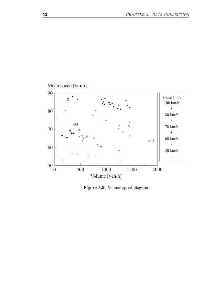
52 CHAPTER 3. DATA COLLECTION
0 500 1000 1500 200050
60
70
80
90
Mean speed [km/h]
Speed limit
100 km/h
80 km/h
70 km/h
60 km/h
50 km/h
12
33
Figure 3.5: Volume-speed diagram

Chapter 4
Identification
4.1 The purpose of identification
A headway (T ) describes the time interval between consecutive vehicles intraffic flow. For a traffic engineer it is interesting to examine the shape andstructure of the headway distribution. The differences between follower andfree flowing headways are of special interest. In capacity and level-of-servicestudies, the proportions of short and long headways deserve attention. Asimulation designer is interested in the possible correlation between consec-utive headways.
Identification is the process of finding, from a set of models, the besttheoretical model to describe the data. It can be a stochastic model or,as here, a probability distribution. An effective description of the mostimportant properties of the data is essential in order to find a theoreticalmodel which has properties similar to the data.
This chapter discusses the shape of the headway distribution, measuresof location and dispersion, and tests for the renewal hypothesis, which areconcerned with the autocorrelation of consecutive headways. Some of themethods (e.g., the hazard function and the KS2-chart) have not been usedin headway studies—at least not widely. For some commonly used methods,more efficient procedures are presented. The concluding section presents afour stage identification process, which is suggested as a standard procedurein headway studies.
53

54 CHAPTER 4. IDENTIFICATION
4.2 Shape of the distribution
4.2.1 Empirical distribution function
The probability distribution function (PDF) defines the probability that aheadway random variate (T ) is not greater than some given value t:
F (t) = P{T ≤ t}. (4.1)
The PDF which has generated a sample of size n can be estimated by the em-pirical distribution function (EDF). It gives the proportion of observationsless than or equal to t in the sample:
Fn(t) ={
j
n
∣∣∣∣ t(j) ≤ t < t(j+1)
}, j = 1, . . . ,n. (4.2)
The EDF has a central role in the goodness-of-fit tests (section 2.2.4).Figure 4.1 shows contour plots of empirical headway distribution func-
tions. Separate plots for low speed (50–70 km/h) and high speed (80–100 km/h) roads were produced by smoothing the sample EDFs. Becausethe traffic volume of only three (low speed) samples is below 200 veh/h, thelow volume contour lines are not very reliable.
The proportion of extremely short headways is small, but between oneand three seconds the EDF rises steeply. On high speed roads the concen-tration on short headways is more substantial than on low speed roads. At500 veh/h the low speed roads have about 30 % of headways shorter thantwo seconds. At the same volume the high speed roads have about 40 % ofheadways shorter than two seconds, and the proportion of short headways israther constant at moderate to high flow rates. The 0.9 contours are almostidentical in both road categories.
At high volumes the contour lines are very densely concentrated at shortheadways, but they curve toward longer headways at lower volumes, thusindicating a greater proportion of long headways. This is only natural, con-sidering that traffic volume is the reciprocal of the mean headway. Accordingto May (1990), the percentage of vehicles having headways less than or equalto the mean headway is rather constant, about 67 %. This approximationholds for the low speed data.
In HCM (1985) the percent time delay is used as a level of service mea-sure. For practical purposes, the percent time delayed is approximated bythe percentage of vehicles traveling in platoons (t < 5). The level of serviceis accordingly based directly on the empirical headway distribution. In fig-ure 4.2 the proportion of vehicles having headways less than five seconds,

4.2. Shape of the distribution 55
Headway [s]
2 6 8 10
500
0
1000
1500
04
Volume [veh/h] Speed limit: 50-70 km/h
2 6 8 10
500
0
1000
1500
04
Headway [s]
Volume [veh/h] Speed limit: 80-100 km/h
Mean headwayMean headway
Figure 4.1: Contour plots of empirical headway distribution functions
is plotted against the traffic volume. Except for two low volume samples(45 and 46), the proportion is larger than in a totally random, or Poisson,process (negative exponential headways). The proportion is also larger onhigh speed roads than on low speed roads.
It should be noted that the data in figure 4.2 are from several sites.Thus, the variation is partly caused by local conditions. However, the figureshows that the data are consistent in respect of the level of service.
Figure 4.3 shows the proportion of headways less than or equal to onesecond. The proportion is 0.11 for high speed roads and 0.062 for low speedroads. There is no significant correlation with the traffic volume. For allbut the lowest volumes, the proportion is lower than in a Poisson process.
Enberg & Pursula (1992) obtained similar results for Finnish high-classtwo-lane roads.1 The data did not indicate a significant correlation betweenvery short (t < 1 s) headways and traffic volume. There is, however, someevidence that on Finnish freeways the proportion of headways less than onesecond increases with increasing traffic volume (Salonen 1982).
1These roads have a very high standard of alignment and grade-separated intersections.The speed limit is 100 km/h, and only fast motor vehicles are allowed.
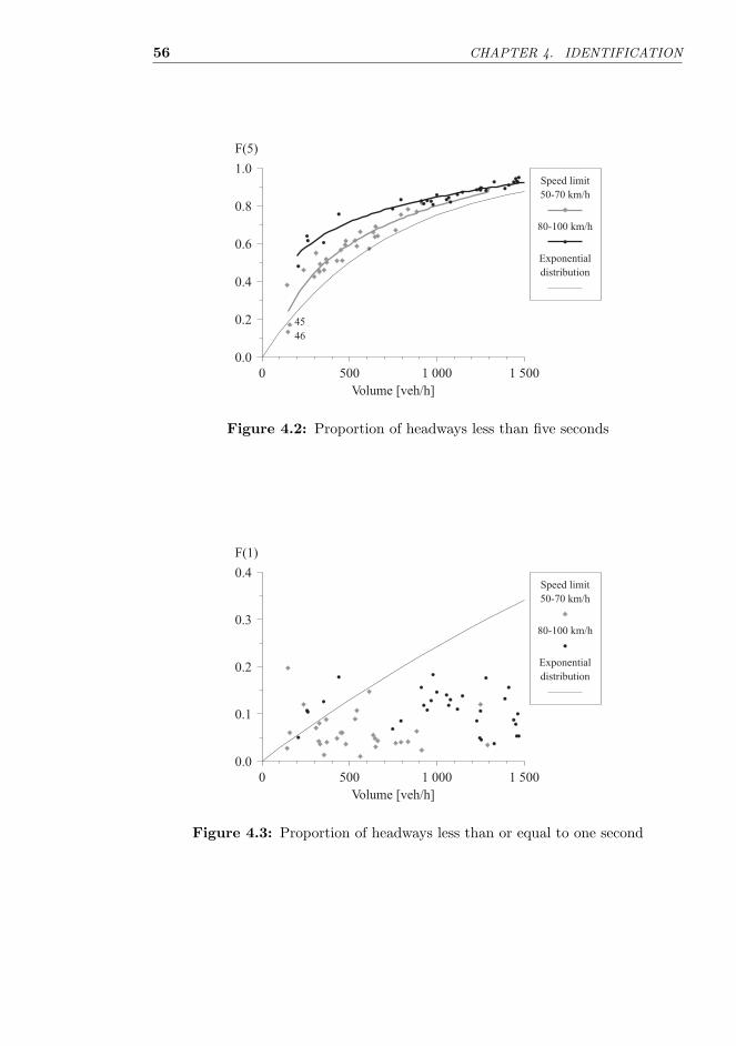
56 CHAPTER 4. IDENTIFICATION
0 500 1 000 1 500
0.0
0.2
0.4
0.6
0.8
1.0
F(5)
Speed limit
50-70 km/h
80-100 km/h
Exponential
distribution
45
46
Figure 4.2: Proportion of headways less than five seconds
0 500 1 000 1 500
0.0
0.1
0.2
0.3
0.4
F(1)
Speed limit
50-70 km/h
80-100 km/h
Exponential
distribution
Figure 4.3: Proportion of headways less than or equal to one second

4.2. Shape of the distribution 57
4.2.2 Empirical density function
The probability distribution function (PDF) can be defined in terms of theprobability density function (pdf):
F (t) =∫ t
0f(x) dx. (4.3)
Thus, the pdf is the derivative of the PDF, and:∫ ∞
0f(x) dx = 1. (4.4)
Both the PDF and the pdf have the same and complete information aboutthe distribution, but the pdf is visually more informative. Because of this,the plotting of the pdf estimates (empirical density functions, edf’s) is astandard procedure in headway studies.
The density function is usually estimated by the histogram method.Starting from an origin (t0), the range of the data is partitioned into bins(class intervals) having the same width (h), which is also called the windowwidth. The height of the histogram at point t is the number of observationsbelonging to the same bin as t divided by the number of total observations(n) and the bin width (h):
fn(t) =1
nh#{i∣∣ [t0 + jh ≤ t < t0 + (j + 1)h]
∧ [t0 + jh ≤ ti < t0 + (j + 1)h]}
i = 1, . . . , n and j = 0, 1, . . . (4.5)
The total area under the histogram is unity. Once the origin and the binwidth are selected, the method is very straightforward, and there are manyprograms to automate the process.
The histogram method has two major drawbacks: Firstly, the locationof the origin (t0) and the bin width (h) can have a considerable effect onthe shape of the estimate, especially at low values of t. Secondly, the dis-continuity of the histograms causes even more difficulties if the derivativesof the density estimate are needed, or if the density estimate is needed asan intermediate component for other methods. (Silverman 1986)
The histogram method calculates the frequency of observations in a win-dow of width h. The window is first placed at the origin, and then shifted tothe right by its own width. Each observation in the window is given equalweight. Better estimates are, however, obtained if the the window slides

58 CHAPTER 4. IDENTIFICATION
smoothly along the x-axis, and the observations are weighted by an appro-priate smoothing function (kernel). The observations in the middle of thewindow should have greater weight, while the observations near the sides ofthe window should be given less weight. This procedure is called the kernelmethod.
The kernel method produces a continuous estimate of the pdf, avoidingthe pitfalls of the histogram method, but some noise in the tail cannot beavoided without losing essential details. The kernel density estimator withkernel K(·) at point t is defined as:
fn(t) =1
nh
n∑i=1
K
(t − ti
h
). (4.6)
Too small values of h produce noisy estimates. On the other hand, too largevalues smooth away essential details of the density.
For headway data, the estimate should reproduce the sharp peak of thepdf without too much noise in the tail. As the density estimates were furthersmoothed in order to produce the surface plots (figures 4.4 and 4.5), a smallsmoothing parameter (h = 0.3) was selected. This estimator was able toproduce the sharp peak of the density, even though there was some noise inthe tail.
The estimates are based on the Epanechnikov kernel (Silverman 1986):
K(x) =
⎧⎨⎩
34√
5
(1 − 1
5x2), if |x| <
√5
0, otherwise.(4.7)
It is the most efficient kernel function, although the differences between thebest kernels are very small (Silverman 1986).
Figures 4.4 and 4.5 show surface plots of headway density estimates.The surfaces were smoothed by a polynomial fit for each t in the grid. Themethod produces some wavelike nonsmoothness in the t direction of thesurface, but the shape of the density functions is very clear. The method ofdistance weighted least squares was also tried. The surfaces were smoother,but the peak was lower, and it had saddle points in the regions of missingobservations (see Luttinen 1994).
The density is unimodal, bell-shaped and skewed to the right. The pro-portion of headways less than one second is small. The mode is betweenone and two seconds, after which the frequencies diminish in an exponentialway. The most striking difference between the figures is that under low vol-ume conditions the frequency of short headways is much lower on low speed

4.2. Shape of the distribution 59
02
4 6 8 10
Headway [s]
200600
10001400
Volume [veh/h]
0
0.1
0.2
0.3
0.4
0.5
f(t)
02
4 6 8 10
Headway [s]
200600
10001400
Volume [veh/h]
Figure 4.4: Empirical headway density function on low speed (50–70 km/h) roads
02
4 6 8 10
Headway [s]
200600
10001400
Volume [veh/h]
0
0.1
0.2
0.3
0.4
0.5
f(t)
02
4 6 8 10
Headway [s]
200600
10001400
Volume [veh/h]
Figure 4.5: Empirical headway density function on high speed (80–100 km/h)roads

60 CHAPTER 4. IDENTIFICATION
roads. As the volume increases, the frequency of short headways, of course,increases on both road categories.
The difference between the two road categories may be caused by greatervariation in speed differences on high speed roads (fig. 5.30, page 133), dif-ferent road conditions, and differences in the opposite flow level. The lowspeed (50–70 km/h) data were collected near densely populated areas, whereintersection density was higher than on high speed (80–100 km/h) roads.
The edf’s have some similarity with the pdf’s of the gamma and thelognormal distributions. Also, several mixed distributions have similar den-sities. The densities of the negative exponential and the shifted exponentialdistributions are, however, different. These distributions have the great-est density at the shortest headways, whereas the edf increases smoothlyfrom zero to the mode. Consequently, the exponential distributions are notappropriate models for short headways.
4.2.3 Empirical hazard function
The hazard function is widely used in reliability and life data analysis. Itgives the instantaneous failure rate for a system that has not failed until t.The hazard function for a random variable T is defined as:
h(t) = lim∆t→0
P{ t ≤ T < t + ∆t | t ≤ T }∆t
=f(t)
1 − F (t).
(4.8)
The pdf and the PDF can be expressed in terms of the hazard function asfollows:
f(t) = h(t) exp(−∫ t
0h(u) du
)(4.9)
F(t) = 1 − exp(−∫ t
0h(u) du
). (4.10)
The hazard function also has the complete information of the distribution. Ifthe hazard function has a simple shape, it is possible to form a hazard-basedmodel using the equations above.
In terms of traffic flow, the hazard function h(t) is the instantaneoustermination rate of headways conditional upon lasting to time t. Besidesof its theoretical significance, the hazard function shows properties of thedistribution that are not so clearly seen in either the pdf or the PDF.

4.2. Shape of the distribution 61
A crude estimate of the hazard function can be quickly calculated byclassifying the data into intervals of length a, and calculating:
hn(t) =#{ ti | t ≤ ti < t + a }
#{ tj | t ≤ tj } , i,j = 1, . . . ,n. (4.11)
Better estimates can, however, be obtained by the kernel method. Thesmoothed empirical hazard function (ehf) of the headway data was calcu-lated using a biweight kernel (IMSL 1989):
K(x) =
⎧⎨⎩
1516(1 − x2
)2, if |x| < 1
0, otherwise.(4.12)
The smoothed kernel is:
Ks(t − t(i)) =1
αdikK
(t − t(i)
βdik
), (4.13)
where α, β, and k are smoothing parameters, dik is the distance to the kthnearest “failure” from t(i), and t(i) is the ith order statistic of the sample.The smoothing parameters were estimated by a modified maximum likeli-hood method.2 Consequently, the ehf was calculated as follows:
hn(t) =n∑
i=1
1n − i + 1
Ks(t − t(i)), (4.14)
where n is the sample size.Figures 4.6 and 4.7 show surface plots of the empirical hazard functions.
The surfaces are smoothed by making a polynomial fit for each t in the grid.The method produced a little nonsmoothness in the t direction, but theshape is obvious. The method of distance weighted least squares was alsotried. It produced smoother surfaces, but the peak had saddle points in theregions of no observations.
The figures have some common properties: The peak is between 1.5 and2 seconds. It moves slightly to the right, as the volume increases. The peakis low at low volumes, and increases as the volume increases. After the peak,the ehf decreases, until it reaches a constant level. This level is higher athigh volumes.
2IMSL subroutines DHAZEZ and DHAZST were used to estimate the parameters andto calculate the empirical hazard functions.

62 CHAPTER 4. IDENTIFICATION
02
46
810
Headway [s]
200
600
10001400
Volume [veh/h]
0
0.2
0.4
0.6
0.8
h(t)
02
46
810
Headway [s]
200
600
10001400
Volume [veh/h]
Figure 4.6: Empirical headway hazard functions for low speed (50–70 km/h) roads
02
46
810
Headway [s]
200
600
10001400
Volume [veh/h]
0
0.2
0.4
0.6
0.8
h(t)
02
46
810
Headway [s]
200
600
10001400
Volume [veh/h]
Figure 4.7: Empirical headway hazard functions for high speed (80–100 km/h)roads

4.2. Shape of the distribution 63
At low volumes the peak is higher on high speed roads. When thevolume on low speed roads is greater than about 1,000 veh/h, the peak risesvery steeply. There are, however, only two low speed samples for volumeshigher than 1,000 veh/h. The extremely high peak is caused by one small(n = 150) sample (no. 52), which has h(2.0) = 1.8. Thus, the high peakshould be viewed with some skepticism. Although the ehf in figure 4.6 isnonsmooth at high volumes, the basic shape is obvious.
The hazard function of the exponential distribution is constant, and equalto the flow rate. The exponential tendency of low volume traffic is evidenton low speed roads; the ehf becomes more level as the volume decreases.
If the tail of the distribution is exponential, the hazard function reachesa constant value at long headways. This value is proportional to the flowrate. Constant ehf values at large headways are accordingly an indicationof an exponential tail in the headway distribution.
The hazard rate of the gamma distribution is monotone decreasing frominfinity if the shape parameter (α) is less than unity, monotone increasingfrom zero if α is greater than unity, and in both cases approaches a constantvalue (scale parameter β) as t becomes large (Kalbfleisch & Prentice 1980).If the shape parameter is α = 1, the distribution is exponential, and thehazard function remains constant [h(t) = β ]. This kind of shape is seenat the lowest volumes on low speed roads, except for the low peak in theehf. This suggests that at low volumes the headway distribution resemblesa gamma distribution, and the shape parameter (α) approaches unity fromabove, as the flow rate decreases to zero. Because h(0) = 0 for α > 1, thegamma distributions do not produce extremely short headways, and becauseh(t) approaches β as t becomes large, the tail of the distributions approachesexponentiality.
The lognormal hazard function is zero at t = 0, increases to maxi-mum, and then decreases, gradually approaching zero at long headways(Kalbfleisch & Prentice 1980). The basic shape is similar to the ehf, but thefall after the peak is more gradual.
The hazard function of the semi-Poisson distribution is similar to theheadway hazard function estimate. The model in figure 5.49 (page 160) hasgamma distributed short headways and exponential tail.
In conclusion, the ehf suggests a mixed distribution with an exponentialtail as a theoretical headway distribution. The lognormal distribution hasdesirable properties at short headways only. The gamma distribution couldbe considered for low volumes.

64 CHAPTER 4. IDENTIFICATION
4.3 Measures of location and dispersion
4.3.1 Mode and peak height
The mode (Mo) is the point where the density reaches its maximum. So, itis an approximation of the most frequent value in the distribution. Summala& Vierimaa (1980) describe the mode as an approximation of the headwaythat most drivers select when they are following the vehicle ahead. As such,the mode is a measure of typical platoon behavior and a crude estimate ofhighway capacity.
The peak height (Ph) is a measure of the frequency at mode. For uni-modal distributions the mode and the peak height can be defined as:
Mo = {t ∈ Re+∣∣ f(t) = max
x∈Re+f(x)} (4.15)
Ph = f(Mo). (4.16)
The mode and the peak height of the headway data were estimated usingkernel estimates for density. The smoothing parameter of the Epanechnikovkernel (4.7) was h = 0.2. A low smoothing parameter was used, because thedensity was estimated only at the range where the observations were mostdensely concentrated. Consequently, the peak height obtained was higherthan in the density estimates. The golden section search (Gill, Murray &Wright 1981) with absolute precision of 0.01 was used to find the maximumof the edf.
The mode values are shown in figure 4.8. There is no significant cor-relation with flow rate. The mode is about 1.53 (with standard deviationof 0.29) on low speed roads and 1.41 (with standard deviation of 0.22) onhigh speed roads. The difference is, however, not statistically significant at5 % risk level (P = 0.08), according to the t-test. Thus, the mode is a littlebelow 1.5 (95 % confidence region is 1.46–1.48) at both high and low speedroads.
Summala & Vierimaa (1980) measured the modes of headway distribu-tions on two-way two-lane roads with speed limits 50–100 km/h. The modevaried between 1.0 and 1.9, but it was rather constant at all traffic volumes.Rajalin & Hassel (1992) studied net time interval (gap) distributions ontwo-way two-lane roads with speed limits 80 km/h and 100 km/h. Theyreported a mode of 0.8 s at all traffic volumes.
The peak heights are shown in figure 4.9. The peak rises as the flowincreases. On high speed roads (speed limit 80–100 km/h) the peak is higherthan on low speed roads, especially at low volumes. At high volumes thespeed limit looses its significance.

4.3. Measures of location and dispersion 65
0 500 1 000 1 500
0.0
0.5
1.0
1.5
2.0
2.5
3.0
Mode [s]
Speed limit
50-70 km/h
80-100 km/h
Figure 4.8: Mode of empirical headway distributions
0 500 1 000 1 500
0.0
0.1
0.2
0.3
0.4
0.5
0.6
Peak height
Speed limit
50-70 km/h
80-100 km/h
Exponential
distribution
45
46
Figure 4.9: Peak height of empirical headway distributions

66 CHAPTER 4. IDENTIFICATION
A regression analysis was performed by means of a logarithmic regression[a + b ln(λ)] for low speed roads and a power regression (aλb) for high speedroads. The fit is reasonable: R2 = 0.737 on low speed roads and R2 = 0.620on high speed roads. The equality of residual means between high speedand low speed roads was tested using the t-test. The hypothesis shouldbe rejected on risk level P = 0.002. The exclusion of the two very low(< 0.05) peak values (samples 45 and 46) makes the result statistically moresignificant (P = 0.001). Similar result (P = 0.007) was obtained usinganalysis of covariance (ANCOVA). Accordingly, separate models should bepresented for lower and upper speed levels.
Enberg & Pursula (1991) reported only small differences in peak heightson high-class two-lane rural roads in Finland. The sampling period was 15minutes. The mode was in the interval 1–2 s. When 60 minute sampleswere used, the increase in the peak height was more evident (Enberg &Pursula 1992).
4.3.2 Median
The median (Md) of a continuous random variate is the 50th percentile ofthe distribution:
P{T ≤ Md} = 0.5. (4.17)
The sample median is a value such that half of the sample observations areto the left and half to the right of it:
Md =
{t(k), if n = 2k − 112
(t(k) + t(k+1)
), if n = 2k.
(4.18)
where t(k) is the kth order statistic of the sample, and n is the sample size.Sample medians of the headway data are shown in figure 4.10. The medianon high speed roads is surprisingly level (R2 = 0.462), but there are onlyfew low volume samples. On low speed roads the volume and the medianare more clearly correlated (R2 = 0.855).
For symmetrical unimodal distributions the mean, the median and themode coincide. It is a known property of nonsymmetric unimodal distri-butions that the mean, the median, and the mode occur in the same orthe reverse order as in the dictionary, and that the median is nearer to themean than to the mode (Stuart & Ord 1987). Because the headway pdf ispositively skewed, these measures occur in the reverse dictionary order.

4.3. Measures of location and dispersion 67
0 500 1 000 1 500
0
5
10
15
20
Headway [s]
Median
50-70 km/h
80-100 km/h
Mean
Figure 4.10: Median of empirical headway distributions
According to Stuart & Ord (1987) the following approximate relationholds for unimodal probability distributions of moderate asymmetry:
Md − Mo ≈ 3[ µ(T ) − Md ]. (4.19)
The headway distribution is, however, too asymmetric for this relation tohold, and the relation gives too high estimates of the median. The linearleast squares estimates are (fig. 4.11):
MdL = 0.529 + 0.465t (4.20)
MdH = 1.601 + 0.107t. (4.21)
The accuracy of the estimate for high speed roads (MdH) is, however, sus-pect, because there are only few low volume observations. The coefficient ofdetermination is only R2 = 0.520 for MdH , as compared to R2 = 0.825 forMdL.
Separate models were estimated for low and high speed roads, althoughANCOVA gave significance probability of only P = 0.059 for the homogene-ity of slopes. The figure, however, shows that the slopes of the regressionlines are quite different, but most of the points from the high speed roadsare near the intersection of the lines. In order to stabilize the variance, aweighting factor of 1/t2 was used. The R2 for the weighted values was 0.966for the low speed data and 0.990 for the high speed data. The adjustedsignificance probabilities were P < 0.001 and P = 0.002, respectively. Theregression is accordingly statistically significant for both data sets.

68 CHAPTER 4. IDENTIFICATION
0 5 10 15 20 25 30
0
5
10
15
20
Median
Speed limit
50-70 km/h
80-100 km/h
Symmetrical
distribution
Figure 4.11: Mean and median of empirical headway distributions
4.3.3 Coefficient of variation
The coefficient of variation (c.v.) is the proportion of the standard deviationto the mean of a random variable (T ):
C(T ) =σ(T )µ(T )
. (4.22)
The sample c.v. is the proportion of the sample standard deviation to thesample mean:
C =s
t. (4.23)
The negative exponential distribution (headway distribution of a totallyrandom arrival process) has C(T ) equal to unity. Because the negativeexponential distribution is central in the theory of stochastic processes, andit is widely applied in traffic flow theory, C(T ) = 1 provides a convenientpoint of comparison.
The CV-chart in figure 4.12 shows the sample coefficients of variationfor the headway data. Some basic properties can be observed:
1. Under heavy traffic conditions, the proportion of freely moving vehiclesis small. The variance of headways is accordingly small. In figure 4.12,the c.v. decreases below unity at high flow levels.

4.3. Measures of location and dispersion 69
0 500 1 000 1 500
0.0
0.5
1.0
1.5
2.0
2.5
Coefficient of variation
Speed limit
50-70 km/h
80-100 km/h
Exponential
distribution
Figure 4.12: CV-chart (sample coefficient of variation) of the headway data
2. The Poisson tendency of low density traffic has a theoretical (Breiman1963, Heidemann 1990) as well as an intuitive basis: Under low densityconditions, the vehicles can move freely, and randomness of the processincreases. Hence, the c.v. is expected to approach unity as the trafficflow approaches null. This phenomenon can be observed only at lowspeed roads, where more low volume samples are available.
3. Under medium traffic, there is a mixture of free-flowing vehicles andfollowers. This increases the variance above pure random process.Accordingly, the c.v. rises above unity. This is in contrast to thestatement of May (1990) that the c.v. approaches unity under lowflow conditions, but decreases continuously as the flow rate increases.According to Pursula & Sainio (1985) the result of May is valid forthe first lane on a freeway.
4. The c.v. is larger on high speed roads than on low speed roads. Inthese data, the opposite flow rate was higher on high speed roads,thus reducing passing opportunities. Other explaining factors maybe higher variation of speeds and greater willingness to pass on highspeed roads. In addition, the intersection density was higher on thelow speed roads. Consequently, there were more joining and departingvehicles, thus reducing the platooning.
To test whether it is appropriate to model the C(T ) on high speed andon low speed roads separately, a third degree polynomial curve was fit to the

70 CHAPTER 4. IDENTIFICATION
c.v. data. The equality of the means of the residuals for high speed and lowspeed roads were tested using a t-test. Using residuals instead of actual c.v.values, increases the power of the test, because the effect of traffic volumecan be circumvented. The equality of the means should be rejected at risklevel 2.2 · 10−6. Because there was a significant difference between the c.v.values on high speed and low speed roads, a separate model was construedfor both.
Two polynomial curves were fitted on the data (figure 4.12): one forthe high speed (80–100 km/h) roads and the other for the low speed (50–70 km/h) roads. The regression equations are:
CL = −7.667λ2 + 2.247λ + 1 (4.24)
CH = (1 − 1.8λ)(1 + 20.173λ − 82.189λ2 + 114.839λ3). (4.25)
The coefficient of determination for the mixed model is R2 = 0.685. That is,about 69% of the variance in the c.v. can be explained by the traffic volume.A single model for all speed limits has R2 = 0.226. Modeling high speedand low speed roads separately explains about 46% more of the variance.
There are some points worth consideration in the equations. The curveswere forced to unity when the traffic volume was zero. This was based onthe assumption of the Poisson tendency in low density traffic. The uppercurve was forced to zero at volume 2,000 veh/h in order to prevent extensivecurviness.
The curves have maxima at flow rates 530 veh/h (low speed roads) and440 veh/h (high speed roads). This corresponds to mean headways 6.8 s and8.2 s. Under lower flow rates, the long headways predominate and reducethe c.v. Traffic density is low, and there are ample opportunities for passing.Under higher flow rates, short headways predominate and reduce the c.v.Drivers are more content to follow in platoons (Pursula & Sainio 1985).Thus, the maximum is likely to be connected with the passing behavior. InBureau of Public Roads (1950) it was shown that typically the demand forpassing becomes greater than the opportunities at flow rate 500 veh/h (seealso Wardrop 1952).
These observations gain at least partial support from other authors, asseen in figure 4.13, although the results are based on very different data.The data of Dunne et al. (1968) are from a two-lane rural road, but thedata of Breiman et al. (1977), Buckley (1968) and May (1965) come fromfreeway lanes. The traffic volumes in all the samples of May are higher thanin the samples of Dunne et al. (1968).
The traffic volumes in the samples of Dunne et al. (1968) are between 350

4.3. Measures of location and dispersion 71
0 500 1 000 1 500 2 0000.0
0.5
1.0
1.5
Coefficient of variation
Dunne
Buckley
May
Breiman
Lane 1
Lanes 2&3
Griffiths
Figure 4.13: Coefficient of variation in other headway studies: Dunne et al.(1968), Buckley (1968), May (1965), Breiman et al. (1977), and Grif-fiths & Hunt (1991)
and 700 veh/h; i.e., the volume range that has the highest c.v. values in figure4.12. In accordance with these results, all the samples of Dunne et al. havec.v. greater than unity. The c.v. is less than unity in the freeway samples ofMay (1965) and Breiman et al. (1977) (lanes one and two), and near unity inthe samples of Buckley (1968) and Breiman et al. from freeway lane three.The data of Buckley represent a wide variety of volume levels, and the c.v.is similar to the results for the low speed roads in figure 4.12. The dataof May were measured for gap availability studies near freeway ramps, andresults are very different from the others. More general conclusions from thedata of May should be drawn only with great care.
Griffiths & Hunt (1991) have studied headways on urban areas. Theyfound a linear relation between the standard deviation and the mean head-way, which can be expressed in terms of the sample c.v. and the trafficvolume (λ, veh/h):
C = 1.07 +0.160λ
3600. (4.26)
This line is shown in figure 4.13.
Finnish studies by Pursula & Sainio (1985) suggest that the c.v. onfreeways, especially on the first lane, is lower than on two-lane highwayswith speed limit 80–100 km/h. The results of Breiman et al. (1977) also

72 CHAPTER 4. IDENTIFICATION
show that lane one has lower c.v. than lane two, which has lower c.v. thanlane three.
4.3.4 Skewness and kurtosis
The proportion of the first two moments was discussed above. The third andthe fourth central moments, skewness (α3) and kurtosis (α4), give us moreinformation about the shape of the distribution. Skewness is a measureof symmetry. For symmetric distributions α3 = 0. If the data are moreconcentrated on the low values, as in a headway distribution, skewness ispositive. Kurtosis is a measure of how “heavy” the tails of a distributionare. Sample skewness and kurtosis are defined as follows:
α3 =∑n
i=1(ti − t )3
ns3 (4.27)
α4 =∑n
i=1(ti − t )4
ns4 . (4.28)
where t and s are sample mean and standard deviation, respectively.The skewness of the headway data is displayed in figure 4.14. Analysis
of covariance shows that the skewness of headway distributions on low speedand high speed roads differs significantly (P < 0.001). Consequently, thelinear regression analysis was performed separately for the low speed and thehigh speed data. On low speed roads the linear model explains 36 % (R2 =0.36) of the variance, and the significance of the regression is P < 0.001.On high speed roads the respective values are R2 = 0.073 and P = 0.136,indicating that the correlation is not significant, and the skewness is about4.05, irrespective of the traffic volume.
On low speed roads, the skewness is near two at low volumes. Thiscorresponds to the skewness of the negative exponential distribution. Athigher volumes the skewness increases.
Following Ramberg, Tadikamalla, Dudewicz & Mykytka (1979), figure4.15 shows the sample kurtosis against the squared sample skewness. (Thefigure is called here a KS2-chart.) This relation is occasionally used as aguide in selecting theoretical distributions (Cochran & Cheng 1989). Therelation in the KS2-chart is almost linear, but a slightly better fit (R2 =0.981) was obtained by the power curve:
α4 = 2.297(α23)
0.847. (4.29)
For comparison, figure 4.15 shows also corresponding points and curves ofsome theoretical distributions. The negative exponential distribution (along

4.3. Measures of location and dispersion 73
0 500 1 000 1 500
0
2
4
6
8
10
Skewness
Speed limit
50-70 km/h
80-100 km/h
Figure 4.14: Sample skewness
0 5 10 15 20 25 30
0
10
20
30
40
50
Kurtosis
Speed limit
50-70 km/h
80-100 km/h
50-100 km/h
Lognormal
Gamma
E
N
U
Abbreviations:
E = Exponential
N = Normal
U = Uniform
Figure 4.15: KS2-chart (kurtosis and squared skewness) of the headway data andsome theoretical distributions

74 CHAPTER 4. IDENTIFICATION
with normal and uniform distributions) reduces to a single point. As thesquared skewness grows the kurtosis grows more slowly than in the case ofeither the gamma or the log-normal distribution, but the gamma distributionis more close to the observed values. The strong correlation of the squaredskewness and the kurtosis motivates a further search for the theoreticalheadway distribution.
4.4 Tests for the renewal hypothesis
4.4.1 Background
According to the renewal hypothesis, the headways are independent andidentically distributed (i.i.d.):
H0 : P{ Ti ≤ t |T1, . . . ,Ti−1 } = P{Ti ≤ t} = F(t) , i = 2,3, . . . (4.30)
and
P{T1 ≤ t} = F(t) . (4.30a)
Such a stochastic process is called an ordinary renewal process. If the firstheadway (T1) has a different probability distribution, the process is calleda modified renewal process. In the headway data under study, the firstheadway in the sample is measured from an arbitrary arrival (synchronizedsampling). Consequently, the first headway can be assumed to have thesame distribution as the other headways.
The alternative hypothesis is that the headways are mutually correlated:If a short (long) headway has a higher probability after previous short (long)headways the data has positive autocorrelation. If a short (long) headway ismore probable after long (short) headways the autocorrelation is negative.If the headways can be assumed i.i.d., the statistical analysis and modelingof vehicle headways is much less complicated.
At low flow rates, with only small differences in desired speeds and goodpassing opportunities, the vehicles can move freely, and correlation betweenconsecutive headways is unlikely. At high flow rates, with large variationin desired speeds and restricted passing opportunities, platooning increases.Because the speeds of the followers are restricted, the platoons are likelyto grow. A short headway is then more likely followed by another shortheadway. This makes the hypothesis of positive correlation plausible. Onthe other hand, negative autocorrelation would appear in such conditions

4.4. Tests for the renewal hypothesis 75
which favor platoons of size two (each leader has one follower). This situationcould realize, when both the demand and the opportunities for passing are“reasonable”. Otherwise the hypothesis of negative autocorrelation is notjustifiable. Consequently, positive autocorrelation should be considered asan alternative to the renewal hypothesis.
If consecutive headways are positively correlated, short and long head-ways are not randomly distributed, but clustered. This can be tested by theruns test. In addition, the positive autocorrelation affects the distribution ofplatoon sizes. Consequently, three methods are presented to test the renewalhypothesis for vehicle headway: (1) autocorrelation analysis, (2) runs testsfor randomness, and (3) tests for the distribution of the platoon length. Thisset of three tests was first proposed by Breiman et al. (1969). The powerof these tests is now further enhanced by calculating the combined proba-bilities and the moving probabilities. The combined probabilities of someearlier test results are also presented.
4.4.2 Autocorrelation
The sample autocorrelation (or serial correlation) coefficient gives a measureof correlation between observations at different distances apart. For a sampleof n observations the autocorrelation coefficient at lag k is:
ρk =
∑n−kj=1 (tj − t )(tj+k − t )∑n
j=1(tj − t )2, (4.31)
where
t =1n
n∑j=1
tj . (4.31a)
Note that ρ0 ≡ 1. The sample autocorrelation coefficients are plotted in acorrelogram (see figure 4.16).
In a sample of n observations the autocorrelation coefficients are asymp-totically normally distributed with mean zero and standard deviation 1/n(Brockwell & Davis 1987). Thus, under null hypothesis, approximately 95 %of the coefficients are within bounds ±1.96n−1/2. The dashed lines in figure4.16 show these bounds.
Autocorrelation coefficients give a rough guide, whether the observationsare from a renewal process (ρk = 0, k = 1,2, . . . ). The most importantcoefficient in this respect is ρ1. Figure 4.17 displays ρ1 for each headway

76 CHAPTER 4. IDENTIFICATION
0 1 2 3 4 5 6 7 8 9 10-0.2
0.0
0.2
0.4
0.6
0.8
1.0
Lag
Autocorrelation coefficient
0 1 2 3 4 5 6 7 8 9 10-0.2
0.0
0.2
0.4
0.6
0.8
1.0
Lag
Autocorrelation coefficient
0 1 2 3 4 5 6 7 8 9 10-0.2
0.0
0.2
0.4
0.6
0.8
1.0
Autocorrelation coefficient
0 1 2 3 4 5 6 7 8 9 10-0.2
0.0
0.2
0.4
0.6
0.8
1.0
Autocorrelation coefficient
Sample 32:
n = 390
λ = 795 veh/h
SL = 80 km/h
Sample 25:
n = 900
λ = 1451 veh/h
SL = 80 km/h
Sample 62:
n = 150
λ = 143 veh/h
SL = 70 km/h
Sample 34:
n = 200
λ = 328 veh/h
SL = 50 km/h
Figure 4.16: Correlograms with 0.95 confidence limits
sample. The coefficients have a large variance, but most values are positive.This indicates that there may be some small positive autocorrelation, butlarger samples are needed to detect it.
Two methods have been used to make the evidence stronger: (1) The sig-nificance probabilities of ρ1 for each sample were combined using the movingprobabilities method. (2) Samples were grouped and partial correlation co-efficients for autocorrelation were calculated. The methods and their resultsare described below.
The test for autocorrelation at lag 1 is:
H0 : ρ1 = 0 (4.32)
against
HA : ρ1 > 0. (4.33)
This is a one-sided test in contrast to the two sided tests normally used(Dunne et al. 1968, Breiman et al. 1969, Chrissikopoulos et al. 1982), becauseit is reasonable to assume that platooning causes positive autocorrelation.

4.4. Tests for the renewal hypothesis 77
0 500 1 000 1 500
-0.2
-0.1
0.0
0.1
0.2
0.3
Autocorrelation coefficient, lag 1
Sample
50-70 km/h
80-100 km/h
11
Figure 4.17: Autocorrelation coefficients at lag 1
The test for negative autocorrelation gave clearly nonsignificant values. Theautocorrelation (ρ1) is negative in some small samples only. For sampleslarger than 250 observations, only one negative autocorrelation was found(sample 11: ρ1 = −0.017).
The variation of the significance probabilities over traffic volumes (fig.4.18) is described by the moving probability method (see section 2.2.6). Onhigh speed (80–100 km/h) roads there is significant autocorrelation betweenconsecutive headways. There is, however, a spike in the moving probabilitycurve, which may indicate better passing opportunities in some samples.(Similar, although lower spikes are in figures 4.19 and 4.20.) On low speed(50–70 km/h) roads there is no significant autocorrelation, at least under lowvolumes. The moving probability curve, however, goes down to significantvalues near 900 veh/h.
The combined significance of all high speed samples is about 3 · 10−22,and for all low speed samples 0.04. Consequently, the renewal hypothesisshould be rejected on high speed roads, at least when the traffic volumeis above 500 veh/h. On low speed roads the possibility of autocorrelationshould be considered at high volumes (λ > 900 veh/h).
On high speed roads the combined ρ1 is 0.07. Since largest samples givemore accurate estimates, the sample coefficients were weighted by the samplesizes. The weighted estimate is ρ1 = 0.09, and the 95 % confidence intervalis 0.06–0.12. On low speed roads the coefficient does not differ significantlyfrom zero. Accordingly, the tests indicate a small, but statistically significant

78 CHAPTER 4. IDENTIFICATION
0 500 1 000 1 500
0.0
0.1
0.2
0.3
0.4
0.5
0.6
0.7
0.8
0.9
1.0
Significance
Sample
50-70 km/h
80-100 km/h
Moving probability
50-70 km/h
80-100 km/h
Figure 4.18: Significance of tests for renewal hypothesis against positive autocor-relation (ρ1 > 0), and 9-point moving probabilities
autocorrelation at lag one on high speed roads.The autocorrelation was also tested using the partial correlation coeffi-
cients. The samples of low speed and high speed roads were combined intothree classes: (0, 500], (500, 1000], and (1000, 1500] veh/h. Because eachsample has a different mean headway (t ), there is correlation between head-ways and their sample means rti t = corr(ti, t ). The correlation of headwaysand sample means increases the autocorrelation [ρ1 = corr(ti, ti−1)] in a com-bined sample. The effect of the mean headway can, however, be eliminatedby the partial correlation coefficient (Fisher 1938):
ρ1·t = corr( ti, ti−1 | t ) =ρ1 − rti t rti−1 t [(1 − r2
ti t)(1 − r2
ti−1 t)] 1
2 . (4.34)
The partial correlation coefficient for autocorrelation at lag one gives the au-tocorrelation coefficient, when the mean headway is held constant. Becauserti t and rti−1 t can be assumed equal (rtt), the partial correlation coefficientcan be calculated as:
ρ1·t =ρ1 − r2
tt
1 − r2tt
. (4.35)
The null hypothesisH0 : ρ1·t = 0 (4.36)

4.4. Tests for the renewal hypothesis 79
can be tested using the following test statistic (Fisher 1938):
y =ρ1·t√
1 − ρ21·t
√n − 4, (4.37)
where n is the number of observations in the class. The statistic y followst-distribution with n−4 degrees of freedom.3 The test results are presentedin table 4.1.
Table 4.1: Partial correlation coefficients (ρ1·t)
Volume class n ρ1·t Significance50–70 km/h
0– 500 veh/h 2494 0.017 0.198500–1000 veh/h 2832 0.025 0.092
1000–1500 veh/h 500 0.053 0.1200–1500 veh/h 5826 0.018 0.081
80–100 km/h0– 500 veh/h 580 0.064 0.062
500–1000 veh/h 2361 0.093 3.30 · 10−6
1000–1500 veh/h 7650 0.092 3.94 · 10−16
0–1500 veh/h 10591 0.076 3.24 · 10−15
The partial correlation coefficients do not indicate any significant auto-correlation at lag one on low speed roads. On high speed roads the positiveautocorrelation is extremely significant under volumes 500–1,500 veh/h. Atlower volumes the autocorrelation is not significant, but the calculation isbased on 580 observations only.
The results of the moving probability method and the partial correlationcoefficients are similar. To sum up, the tests indicate that on high speedroads at volumes greater than 500 veh/h the autocorrelation coefficient atlag 1 is about 0.09. Under lower volumes and on low speed roads, there is noevidence of autocorrelation. It should be emphasized that the decisive factormay not be the speed limit, at least alone. Other road conditions, such asthe intersection density and the opposite flow rate may have an impact onthe autocorrelation, as well.
Some earlier results are discussed below. Combined probabilities andone-sided test results have been calculated by the present author on the
3The degrees of freedom are k−3, where k is the number of correlation pairs {ti, ti−1},which is equal to n − 1. This is also true for the rightmost rooted term in the equationfor y.

80 CHAPTER 4. IDENTIFICATION
basis of the original results. Dunne et al. (1968) studied the autocorrelationof trend-free samples from a two-lane road. The combined probability oftheir nine data sets (lag 1) was 0.702 (one-sided test), which is consistentwith the renewal hypothesis. Two-sided test gives 0.284, which is also non-significant. Breiman et al. (1969) found in one of eight data sets (three-laneunidirectional section of John Lodge Expressway in Detroit) significant au-tocorrelation (lag 1) at 0.05 level. The hypothesis of independent intervalswas not rejected. The combined significance is 0.23. Testing for positiveautocorrelation only (one-sided test) the combined significance is 0.05, sug-gesting possible positive autocorrelation. In a later article Breiman et al.(1977) proposed that a small positive correlation between successive spaceheadways may be present. Cowan (1975) studied 1,324 successive head-ways on a two-lane road in Australia. On the basis of the autocorrelationcoefficient and a runs test, the renewal hypothesis was not rejected. Chris-sikopoulos et al. (1982) studied six headway samples from U.K. trunk roads.The result of their unspecified tests was that the headways were indepen-dently distributed. However, the combined significance probability (lag 1)of their data is 0.012 using 2-sided test, and 0.0015, when testing againstpositive autocorrelation.
Previous studies have so far given support to the renewal hypothesis.Further analysis of this material has cast some doubt on the conclusions.Also the new data presented, shows that the possibility of a small positiveautocorrelation between consecutive headways should be taken seriously.Although the autocorrelation is statistically significant, it is virtually in-significant in many applications.
4.4.3 Randomness
Randomness of the headway data was tested using the Wald & Wolfowitz(1940) runs test. It tests, whether long and short headways are randomlydistributed, or if short headways are clustered. Testing runs above andbelow the median (Md) (Madansky 1988) is appropriate in this case (seealso Breiman et al. 1969).
Let each observation ti be associated with a variable xi so that:
xi =
{1, if ti > Md0, if ti < Md .
(4.38)
The observations equal to the median are ignored. A sequence {xj+1,xj+2,. . . , xj+k} is called a run if xj+1 = xj+2 = · · · = xj+k and xj = xj+1

4.4. Tests for the renewal hypothesis 81
0 500 1 000 1 500
0.0
0.2
0.4
0.6
0.8
1.0
Significance
Sample
50-70 km/h
80-100 km/h
Moving probability
50-70 km/h
80-100 km/h
Figure 4.19: Significance probabilities of one-sided runs tests and 7-point movingprobabilities
and xj+k = xj+k+1. The first and the last observation begin and end, re-spectively, a run.
The number of runs is asymptotically normally distributed with meanand variance equal to (Wald & Wolfowitz 1940):
µ =2r(n − r)
n+ 1 (4.39)
σ2 =2r(n − r)[2r(n − r) − n]
n2(n − 1), (4.40)
where n is the total number of observations and r is the number of observa-tions below the median. Clustering reduces the number of runs. The numberof runs is reduced also by a trend in the data. Hence, the trendlessness ofthe data is important.
The one-sided tests for the probability of less runs were used, in orderto test if the platooning reduces the number of runs. Figure 4.19 showsthe significance of the one-sided tests and the moving probabilities (section2.2.6) for high speed and low speed roads. The combined probabilities aredisplayed in table 4.2. The combined probabilities for two-sided tests arepresented for comparison.
On high speed roads the moving probabilities are significant almostthroughout the volume range. On low speed roads the nonrandomness issignificant for volumes greater than 700 veh/h. The combined significance

82 CHAPTER 4. IDENTIFICATION
Table 4.2: Significance probabilities of the runs tests
Speed limit [km/h] One-sided test Two-sided test50–70 0.001 0.07480–100 0.000 0.000
on high speed roads is 1.6 ·10−20 and on low speed roads 0.001. It is evidentthat the headways are not i.i.d., but clustered.
Breiman et al. (1969) found only one significant value (0.03) in eightruns tests. The combined probability (0.49) is also nonsignificant. This iscontrary to the results presented above.
4.4.4 Platoon length
Vehicle (i) is defined to be a follower (0) if its headway is at most t0, oth-erwise it is a leader (1). The status of a vehicle is accordingly defined asfollows:
xi =
{0, if ti ≤ t0
1, otherwise.(4.41)
The difference in speed is ignored.The number of vehicles in a platoon is the number of consecutive gaps
ti ≤ t0 (followers) plus 1 (leader). The platoon has length k if x1 = 1,x2 = 0, x3 = 0, . . . , xk = 0, and xk+1 = 1. The platoon may consist of asingle vehicle (k = 1).
If the headways are i.i.d., the probability of vehicle i being a follower is:
p = P{ti ≤ t0} = F (t0). (4.42)
The platoon length is then geometrically distributed (Drew 1968), and theprobability for length k is:
pk = pk−1(1 − p), k = 1,2, . . . (4.43)
The renewal property (i.i.d. headways) can be tested using the null hy-pothesis:
H0 : pk = pk−1(1 − p) (4.44)
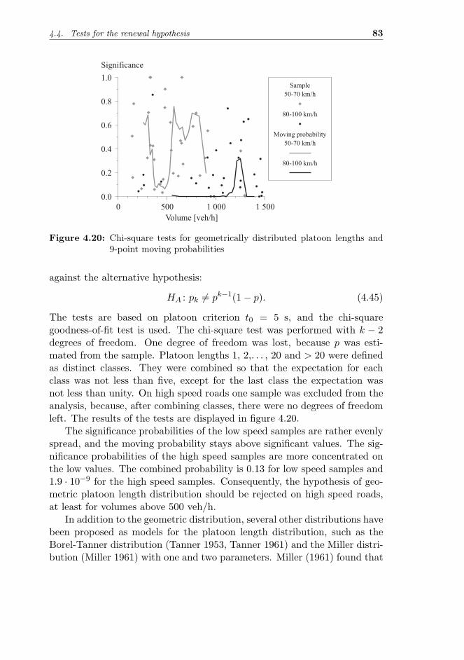
4.4. Tests for the renewal hypothesis 83
0 500 1 000 1 500
0.0
0.2
0.4
0.6
0.8
1.0
Significance
Sample
50-70 km/h
80-100 km/h
Moving probability
50-70 km/h
80-100 km/h
Figure 4.20: Chi-square tests for geometrically distributed platoon lengths and9-point moving probabilities
against the alternative hypothesis:
HA : pk = pk−1(1 − p). (4.45)
The tests are based on platoon criterion t0 = 5 s, and the chi-squaregoodness-of-fit test is used. The chi-square test was performed with k − 2degrees of freedom. One degree of freedom was lost, because p was esti-mated from the sample. Platoon lengths 1, 2,. . . , 20 and > 20 were definedas distinct classes. They were combined so that the expectation for eachclass was not less than five, except for the last class the expectation wasnot less than unity. On high speed roads one sample was excluded from theanalysis, because, after combining classes, there were no degrees of freedomleft. The results of the tests are displayed in figure 4.20.
The significance probabilities of the low speed samples are rather evenlyspread, and the moving probability stays above significant values. The sig-nificance probabilities of the high speed samples are more concentrated onthe low values. The combined probability is 0.13 for low speed samples and1.9 · 10−9 for the high speed samples. Consequently, the hypothesis of geo-metric platoon length distribution should be rejected on high speed roads,at least for volumes above 500 veh/h.
In addition to the geometric distribution, several other distributions havebeen proposed as models for the platoon length distribution, such as theBorel-Tanner distribution (Tanner 1953, Tanner 1961) and the Miller distri-bution (Miller 1961) with one and two parameters. Miller (1961) found that

84 CHAPTER 4. IDENTIFICATION
his one parameter model fitted the data about as well as the Borel-Tannerdistribution. Galin (1980) found the Borel-Tanner and the two-parameterMiller models more accurate than the geometric distribution or the one-parameter Miller model. The headway data were from two-lane Israeli roads.The combined significance probability for the geometric distribution can becalculated as 0.0001. For comparison, the respective probability for theBorel-Tanner distribution is 0.739, for the one parameter Miller distribution0.0007, and for the two parameter Miller distribution 0.889. These resultsconfirm the rejection of the geometric distribution.
4.5 Discussion
After the measurements, trend tests and other preliminary analysis, 63trendless samples consisting of 16,417 headways were analyzed. The sampleswere classified into two road categories according to the speed limit: the lowspeed roads (50–70 km/h) and the high speed roads (80–100 km/h).
The renewal hypothesis was tested using three methods: autocorrelationanalysis, runs tests and tests for geometrically distributed platoon lengths.The significance probabilities of individual samples were combined, and thevariation of significance over different flow levels was described by movingprobabilities. In contrary to many previous papers, the headway data indi-cates that the possibility of a small positive autocorrelation should not beneglected.
A four-stage identification process (Luttinen 1994) is suggested to de-scribe the properties of the headway distribution. This process combinesthe most powerful analyses presented above:
1. The empirical probability density function (edf) shows the basic shapeof the headway distribution more clearly than the empirical distribu-tion function. It should be estimated by a kernel method in order toobtain a continuous estimate, and to avoid the bias due to the his-togram method.
2. The empirical hazard function (ehf) gives even more information aboutthe statistical properties of headways than the edf. A graphical exam-ination of both the edf and the ehf gives a clear indication about theshape of the headway distribution.
3. The moments of a distribution provide some numerical measures forthe identification process. The sample moments may have large varia-tion, but their relations provide proper measures for the identification.

4.5. Discussion 85
The coefficient of variation is a scaled measure of the distributionspread. A CV-chart gives essential information about the headwaydata and proposed theoretical distributions. It is especially worthchecking, whether the coefficient of variation is near, below, or aboveunity.
4. The kurtosis and the squared skewness of the headway samples havea close, linear or quasi-linear relation, which supports their applica-tion in the identification. The KS2-chart shows very effectively thedifferences between theoretical distributions and the data.
The four-stage identification process reveals many shortcomings of thesimple distributions. The exponential distribution does not pass any of theidentification phases. The hazard function and the coefficient of variationreveal the problems of the gamma distribution most clearly. The deviationof the lognormal distribution from the headway data is most obvious, whenthe kurtosis and the squared skewness are measured. The empirical hazardfunction indicates that the tail of the headway distribution is exponential.Consequently, the four-stage identification process suggests mixed distribu-tions with an exponential right tail. The process can be applied to furtherevaluate such models.
The identification process has demonstrated some general properties ofheadways. There is, however, wide variability among the samples and theroad categories. High speed roads have a higher peak in the empirical den-sity and hazard functions, a higher proportion of trailing vehicles, and ahigher coefficient of variation, as well as more significant serial correlationbetween consecutive headways. These differences all relate to the higher pla-tooning on high speed roads, which can be explained by many factors: Thenumber of passing opportunities depends on the headway distribution of theopposite flow. If the passing rate is different from the catch-up rate, the flowis not in equilibrium but in a transition state (McLean 1989). The shape ofthe headway distribution changes, as the measurement point is moved alongthe road. When the passing demand exceeds the passing opportunities, itcan be expected that, moving in the direction of the traffic stream on a lane,the speeds will decrease and the platooning increase (Botma 1986). On anon-uniform road, the equilibrium will not be achieved if the sub-sectionis shorter than the required transition length (McLean 1989). In addition,speed limit, passing sight distance, lane and shoulder width, climbing lanes,flow rate of the opposing traffic,4 intersection density, and distance to major
4When the opposing volume is above 400–450 veh/h, the headway distribution doesnot change relevantly (Heidemann 1993).

86 CHAPTER 4. IDENTIFICATION
traffic generators will have an effect on the headway distributions. Conse-quently, the traffic flow is not stationary in space, but each cross-section oneach road has its own traffic characteristics. A headway model is necessarilya gross simplification of the reality.
The data from high speed roads have been analyzed previously by Pur-sula & Sainio (1985) and Pursula & Enberg (1991). Some comparisons ofthe results are presented below:
1. The density estimates were not calculated by Pursula & Sainio (1985),but frequency diagrams were displayed with bin width 0.5 s and theorigin at zero. Because the frequencies were not corrected by theinterval width, the values were lower by a factor of 0.5, as comparedto the density estimates. The basic shape was, however, the same aspresented here. As Pursula & Sainio (1985) observed, the mode of theheadway distributions is between 1 and 2 seconds.
2. The peak heights are in the same range, when the correction due tothe interval width is made. The comparison with the exponentialdistribution is different, because the correction is not made in figure23 of Pursula & Sainio (1985). If the correction is made, the resultsare very similar.
3. The coefficients of variation have similar values. The c.v. is aboveunity at volumes less than about 1,500 veh/h. In the data of Pursula &Sainio (1985) the c.v. decreases steeply at volumes above 1,200 veh/h.In the present data, the decrease begins gradually and at lower vol-umes.
4. The platoon percentage is similar here as presented by Pursula &Sainio (1985) and Pursula & Enberg (1991). The curve in figure 4.2is, however, in the upper part of the range in figure 24 of Pursula &Sainio (1985), especially at low volumes.
A major reason for the differences may be in the data collection prin-ciple. Trend analysis was not used, but the headways were collectedin 5 minute time slices. Moreover, the proportion of heavy vehiclesand passing vehicles did not have any effect on the data collection. Inthe present analysis, the rejection of measure periods with more than1 % passing vehicles may have favored samples with more vehicles inplatoons and no “holes” in the flow. There may also be differences inthe opposite traffic volumes.

Chapter 5
Theoretical headway models
5.1 Principles of evaluation
The evaluation of the headway distribution models is based on three con-siderations:
1. Reasonability. It is an advantage if the structure of the modelis based on explicit theoretical reasoning about the characteristics oftraffic flow. The parameters of such models can give additional infor-mation on the properties of traffic flow.
2. Applicability. In mathematical analysis the model should have asimple structure to avoid insurpassable problems, and the existenceand simple form of the Laplace transform1 is often an advantage. Ifsimulation is considered as an alternative, the generation of pseudo-random variates should be fast and reliable. Parameter estimationshould not be too complicated.
3. Validity. The model should give a good approximation of the realworld phenomena; i.e., the empirical headway distributions. This istested first by the identification process and finally by the goodness-of-fit tests.
1Laplace transforms, or some other transforms, are commonly used in probability the-ory, because they make many calculations easier. The Laplace transforms can be used toobtain the moments of a distribution (see footnote 5, page 129). When dealing with sumsof random variates, the convolution property of the Laplace transform is most helpful:
f∗X+Y (s) = f∗
X(s)f∗Y (s).
(See Kleinrock 1975, Luttinen 1990).
87

88 CHAPTER 5. THEORETICAL HEADWAY MODELS
Five theoretical distributions were selected for a more detailed analysis:the negative exponential distribution, the shifted exponential distribution,the gamma distribution, the lognormal distribution and the semi-Poissondistribution. The negative exponential distribution is the interarrival timedistribution of a totally random arrival process, i.e. the Poisson process.The shifted exponential distribution avoids the problem of extremely shortheadways by setting a threshold for short headways. The gamma distribu-tion is a generalization of the exponential distributions. A special case ofthe gamma distribution, namely the Erlangian distribution, has been widelyused in the traffic flow theory. The lognormal distribution has a theoreticalconnection to the car-following models (Greenberg 1966). As an exampleof mixed models, the semi-Poisson distribution is studied. It has combinedthe follower headway distribution and the exponential tail most elegantly.Some other mixed models are discussed briefly.
The theoretical models are divided into two classes: the simple distribu-tions and the mixed distributions. The simple distributions have the samemodel for all vehicles. The mixed distributions typically have two distinctheadway distributions: one for free-moving and the other for trailing (fol-lowing) vehicles.
5.2 Simple Distributions
5.2.1 Negative exponential distribution
Properties of the negative exponential distribution
The negative exponential distribution is the interarrival time distributionof the Poisson process. The Markov property2 makes the distribution ana-lytically simple to use. Consequently, the distribution is widely used in thetheory of point processes. In traffic flow theory, the negative exponentialdistribution has been used since Adams (1936).
A process, which has the following four properties, is a Poisson process(Khintchine 1960):
1. The number of events at the beginning of the process is zero; i.e.,N(0) = 0.
2Also called “lack of memory”:
P{ T > t + u | T > t } = P{T > u} .

5.2. Simple Distributions 89
2. The process has independent increments:
P{N(l1,u1] = n1, . . . , N(lr,ur] = nr} =r∏
i=1
P{N(li,ui] = ni}
for all l1 < u1 ≤ l2 < u2 ≤ · · · ≤ lr < ur, r = 1,2, . . . (5.1)
3. The process has stationary increments:
P{N(a,b] = k} = P{N(a + c,b + c] = k}= P{N(b − a) = k} 0 ≤ a < b, c ≥ 0.
(5.2)
4. At any time instant only one event can occur:
P{N(t, t + ∆] ≥ 2} = o(∆) as ∆ → 0. (5.3)
The basic statistical properties of the negative exponential distributionare presented in table 5.1. Concerning the four-stage identification process,the following observations can be made:
1. The negative exponential density function (fig. 5.1) has mode at zero.The peak height is f(0) = λ, after which the density decreases expo-nentially. The distribution overestimates the frequency of extremelyshort intervals and underestimates the frequency of headways nearthe mode of the empirical headway distribution. Longer headways areagain overestimated (fig. 5.2).
2. The hazard rate is equal to the flow rate [h(t) = λ].
3. The coefficient of variation is equal to unity.
4. The skewness and the kurtosis have constant values, independent ofthe scale parameter (λ).
The negative exponential distribution does not pass the four-stage identifi-cation process. In fact, it fails in all four stages.
Parameter estimation
The expectation of the distribution is the reciprocal of the scale parameter(Luttinen 1990). Accordingly, the method of moments estimator (MME) forthe scale parameter (λ) is the reciprocal of the sample mean:
λ =1t. (5.4)

90 CHAPTER 5. THEORETICAL HEADWAY MODELS
02
4 6 8 10
Headway [s]
200600
10001400
Volume [veh/h]
0
0.1
0.2
0.3
f(t)
02
4 6 8 10
Headway [s]
200600
10001400
Volume [veh/h]
Figure 5.1: Negative exponential density function
0 2 4 6 8 100.0
0.1
0.2
0.3
0.4
0.5
Headway [s]
Sample 32:
n = 390
λ = 795 veh/h
SL = 80 km/h
P(A-D) = 0.000
P(K-S) = 0.000
0 2 4 6 8 100.0
0.1
0.2
0.3
0.4
0.5
Headway [s]
Exponential pdf
0 2 4 6 8 100.0
0.1
0.2
0.3
0.4
0.5 Sample 62:
n = 150
λ = 143 veh/h
SL = 70 km/h
P(A-D) = 0.000
P(K-S) = 0.000
0 2 4 6 8 100.0
0.1
0.2
0.3
0.4
0.5 Sample 34:
n = 200
λ = 328 veh/h
SL = 50 km/h
P(A-D) = 0.000
P(K-S) = 0.000
Sample 25:
n = 900
λ = 1439 veh/h
SL = 80 km/h
P(A-D) = 0.000
P(K-S) = 0.000
Sample edf
Figure 5.2: Negative exponential pdf’s and sample edf’s

5.2. Simple Distributions 91
Table 5.1: Properties of the negative exponential distribution
PDF F (t) =
{1 − e−λt, if t ≥ 00, otherwise
pdf f(t) =
{λe−λt, if t ≥ 00, otherwise
Hazard function h(t) =
{λ, if t ≥ 00, otherwise
Laplace transform f∗(s) =λ
s + λ
Mean µ(T ) =1λ
Median Md =1λ
ln 2
Mode Mo = 0
Variance σ2(T ) =1λ2
Coefficient of variation C(T ) = 1
Skewness α3(T ) = 2
Kurtosis α4(T ) = 9
λ > 0
The likelihood function and the loglikelihood function are:
L(λ) = λne−λ∑n
j=1 tj (5.5)
lnL(λ) = n lnλ − λ
n∑j=1
tj . (5.6)
The maximum likelihood estimator (MLE) is obtained by differentiation
∂ lnL(λ)
∂λ=
n
λ−
n∑j=1
tj = 0 (5.7)
λ =1t. (5.7a)

92 CHAPTER 5. THEORETICAL HEADWAY MODELS
0 500 1 000 1 500
0.0
0.2
0.4
0.6
0.8
1.0
Volume [veh/h]
P(A-D)
50-70 km/h 80-100 km/h
0 500 1 000 1 500
0.0
0.2
0.4
0.6
0.8
1.0
Volume [veh/h]
P(K-S)
50-70 km/h 80-100 km/h
45
45
46
46
Figure 5.3: The nonparametric K-S and the parametric A-D goodness-of-fit testsfor the negative exponential distribution
The MLE and the MME are identical for the negative exponential distribu-tion. This estimator has been used in the following statistical analyses.
Goodness-of-fit tests
The goodness of fit was tested using the parametric Anderson-Darling (A-D)test. For each sample 9,999 replications were generated and analyzed. Figure5.3 shows the test results. For comparison, the results of nonparametricKolmogorov-Smirnov (K-S) tests are also presented.
The combined significance probability of the A-D tests is practically zero(2.9 · 10−150). Even for the three low volume (less than 160 veh/h) samples,the combined significance is 0.00016. Only two small samples (45 and 46) ofno more than 100 observations yield nonsignificant results. Consequently,the negative exponential distribution should be rejected, at least for volumesgreater than 140 veh/h.

5.2. Simple Distributions 93
Negative exponential distribution in headway studies
Reasonability The Poisson process describes situations, where vehicleswithout physical length can move freely. Several authors (e.g., Weiss &Herman 1962, Breiman 1963, Thedeen 1964) have shown that under ratherweak assumptions (no driver interactions and i.i.d. speeds) the number ofvehicles in an arbitrary interval will be asymptotically Poisson distributedas time tends to infinity. Thus, the headways will asymptotically follow thenegative exponential distribution. This is called the Poisson tendency oflow density traffic.
Some platooning nearly always occurs on two lane roads, because passingis restricted, and even in good passing conditions some drivers are contentto follow behind. The Poisson process cannot deal with this phenomenon.
Applicability Because of the Markov property, the negative exponentialdistribution lends itself to demanding mathematical analyses. A further ad-vantage is the simple form of the Laplace transform. Therefore, the negativeexponential distribution is often preferred over other, more realistic but alsomore complex distributions. In many cases explicit solutions can only befound, when the arrival process is assumed Poisson.
Because the traffic volume is the only information needed, the parame-ter estimation is very straightforward. Also, the generation of exponentialrandom variates is very effective. Hence, the applicability of the negativeexponential distribution is excellent.
Validity The frequency of unrealistically short headways in the negativeexponential distribution is too large. In fact, extremely short headways havethe highest probability density. The model gets more distorted as the flowrate increases (fig. 5.2).
On the basis of the Poisson tendency theory, the exponential distributioncould be used in the study of low density traffic conditions. Wattleworth (inBaerwald 1976) suggests flow rates of 500 veh/h or less. The coefficient ofvariation data and the goodness-of-fit tests above suggest even lower volumes(about 100 veh/h or less). There is, however, not enough low volume datato make accurate recommendations.
The negative exponential distribution has since Adams (1936) played amajor role in the theoretical study of traffic flow, and especially in trafficsignal control. The studies of Garwood (1940), Darroch et al. (1964), andmany others rely on the exponential headway distribution. Also in somemodern studies on adaptive traffic signal control, the queue length predictor

94 CHAPTER 5. THEORETICAL HEADWAY MODELS
algorithm is based, at least partially, on Poisson arrivals (Baras, Levine &Lin 1979b, Betro, Schoen & Speranza 1987).
In conclusion, the negative exponential distribution can be considered asa model for vehicle headways under very low flow conditions and for appli-cations that are not very sensitive to the shape of the headway distribution.In some cases the analytical solution of the problem may only be possiblewith a very simple model. In such situations the limitations of the modelshould be clearly indicated.
5.2.2 Shifted exponential distribution
Properties of the shifted exponential distribution
One possibility to avoid the extremely short headways predicted by thenegative exponential distribution is, in queuing theory terminology, to add aphase with deterministic service time (τ) in series with the exponential server(Luttinen 1990). This is equivalent to shifting the negative exponentialdistribution τ seconds to the right. A headway is then considered as arandom variate T = τ + X, where τ is a nonnegative constant, and X is arandom variate following the negative exponential distribution.
The density function is obtained from the negative exponential pdf byreplacing t with t − τ :
f( t | τ, θ ) =
{θe−θ(t−τ), if t ≥ τ
0, otherwise,(5.8)
where τ and θ are the location and scale parameters, respectively.The basic statistical properties of the shifted exponential distribution
are presented in table 5.2. Concerning the four-stage identification process,the following observations can be made:
1. The pdf (fig. 5.4) has mode at τ with peak height f(τ) = θ, afterwhich the density decreases exponentially. Figure 5.5 shows the shiftedexponential pdf estimates for four headway samples. The pdf under-estimates the density near the sample mode, and overestimates thefrequency of long headways.
2. The hazard rate is equal to the scale parameter; i.e., h(t) = θ for t ≥ τ .
3. In terms of flow rate [λ = 1/µ(T )], the coefficient of variation isC(T ) = 1 − λτ . Because the location parameter is always nonneg-ative (τ ≥ 0), the c.v. is less than or equal to unity.

5.2. Simple Distributions 95
Table 5.2: Properties of the shifted exponential distribution
PDF F (t) =
{1 − e−θ(t−τ), if t ≥ τ
0, otherwise
pdf f(t) =
{θe−θ(t−τ), if t ≥ τ
0, otherwise
Hazard rate h(t) =
{θ, if t ≥ τ
0, otherwise
Laplace transform f∗(s) = e−sτ θ
s + θ
Mean µ(T ) = τ +1θ
Median Md = τ +ln 2θ
Mode Mo = τ
Variance σ2(T ) =1θ2
Coefficient of variation C(T ) =1
1 + θτ
Skewness α3(T ) = 2
Kurtosis α4(T ) = 9
θ > 0, τ ≥ 0
4. The skewness and the kurtosis have constant values, independent ofthe parameters.
The shifted exponential distribution does not pass the identification process.Like the negative exponential distribution, it fails in all the four stages.
Parameter estimation
Method of moments estimators The method of moments estimators(MMEs) are obtained by equating the expressions for the mean and thevariance (table 5.2) to the sample mean (t) and the sample variance (s2):
t = τ +1θ
(5.9)

96 CHAPTER 5. THEORETICAL HEADWAY MODELS
02
4 6 8 10
Headway [s]
200600
10001400
Volume [veh/h]
0
0.2
0.4
0.6
f(t)
02
4 6 8 10
Headway [s]
200600
10001400
Volume [veh/h]
Figure 5.4: Shifted exponential density function
0 2 4 6 8 100.0
0.1
0.2
0.3
0.4
0.5
Headway [s]
Sample 32:
n = 390
λ = 795 veh/h
SL = 80 km/h
P(A-D) = 0.000
P(K-S) = 0.000
0 2 4 6 8 100.0
0.1
0.2
0.3
0.4
0.5
Headway [s]
Shifted exp. pdf
0 2 4 6 8 100.0
0.1
0.2
0.3
0.4
0.5 Sample 62:
n = 150
λ = 143 veh/h
SL = 70 km/h
P(A-D) = 0.000
P(K-S) = 0.000
0 2 4 6 8 100.0
0.1
0.2
0.3
0.4
0.5 Sample 34:
n = 200
λ = 328 veh/h
SL = 50 km/h
P(A-D) = 0.000
P(K-S) = 0.000
Sample 25:
n = 900
λ = 1439 veh/h
SL = 80 km/h
P(A-D) = 0.000
P(K-S) = 0.000
Sample edf
Figure 5.5: Shifted exponential pdf’s and sample edf’s

5.2. Simple Distributions 97
s2 =1θ2
. (5.10)
By solving this pair of equations the MMEs are obtained as:
τ = t − s (5.11)
θ =1s
=1
t − τ. (5.12)
If the sample c.v. is greater than unity, the sample standard deviation(s) is greater than the sample mean (t). The location parameter estimate isthen infeasible (τ < 0), and the best estimate, in the sense of the method ofmoments, is τ = 0, which leads to the negative exponential distribution.
Modified method of moments estimators The first order statistic(T(1)) in a sample of size n from a shifted exponential distribution f( t | τ, θ )follows the shifted exponential distribution with the scale parameter equalto nθ (Cohen & Whitten 1988). Thus:
f(t(1) | τ, nθ
)=
{nθe−nθ(t(1)−τ), if t(1) ≥ τ
0, otherwise.(5.13)
T(1) has expectation:
E(T(1)) = τ +1nθ
. (5.14)
The estimating equations of the modified method of moments estimators(MMMEs) are then:
E(T ) = t = τ +1θ
(5.15)
E(T(1)) = t(1) = τ +1nθ
. (5.16)
The MMMEs are now obtained as follows:
τ =nt(1) − t
n − 1(5.17)
θ =1
t − τ. (5.18)
According to Cohen & Whitten (1988) these are both the best linear un-biased estimators (BLUE) and the minimum variance unbiased estimators(MVUE), and therefore they are the preferred estimators.

98 CHAPTER 5. THEORETICAL HEADWAY MODELS
0 500 1 000 1 500
0.0
0.2
0.4
0.6
0.8
1.0
1.2
1.4
Location parameter
Speed limit
50-70 km/h
80-100 km/h
46
45
Figure 5.6: MMMEs for the location parameter of the shifted exponential distri-bution
Figure 5.6 shows the MMMEs for τ . The estimates do not correlate withthe volume. The mean of the estimates is 0.63 s on low speed roads and0.38 s on high speed roads. The difference in the estimates is statisticallysignificant (P < 0.0005). The two estimates (samples 45 and 46) greaterthan one second must be considered outliers due to small sample sizes (n ≤100). If they are removed, the mean for the low speed roads is 0.59 s, whichis still significantly larger than the mean for high speed roads.
Maximum likelihood estimators The likelihood function and its loga-rithm for the shifted exponential distribution are:
L(τ, θ) =
{θne− ∑n
j=1 θ(ti−τ), if t(1) ≥ τ
0, otherwise(5.19)
lnL(τ, θ) =
{n ln θn −∑n
j=1 θ(ti − τ), if t(1) ≥ τ
−∞, otherwise.(5.20)
For any fixed θ, the likelihood function is maximized by choosing τ aslarge as possible so that:
f( ti | τ, θ ) > 0 for all i = 1, . . . , n. (5.21)
This leads to:τ = min{t1, . . . , tn} = t(1). (5.22)

5.2. Simple Distributions 99
If the location parameter estimate τ is known, the scale parameter estimate(θ) is obtained by solving (Dudewicz & Mishra 1988):
∂L(τ , θ)
∂θ=
n
θ−
n∑i=1
(ti − τ) = 0, (5.23)
which gives:
θ =1
t − τ. (5.24)
Because the probability P{T ≤ t(1)
}= F(
t(1)
∣∣∣ θ, τ ) is null, the MLEs givebad goodness-of-fit test results.
Modified maximum likelihood estimators The modified maximumlikelihood estimate (MMLE) for τ is calculated from the following equation:
F(t(1)∣∣ τ , θ
)=
1n + 1
. (5.25)
The estimator for θ is the same as given by the maximum likelihood method,as well as by the other methods. The MMLEs are accordingly:
τ =ln(
nn+1
)t + t(1)
ln(
nn+1
)+ 1
(5.26)
θ =1
t − τ. (5.27)
For sample sizes near and above 100, the MMLEs are virtually equal to theMMMEs. The MMMEs were used, because they could be calculated moreeffectively.
Goodness-of-fit tests
The goodness of fit was tested using the parametric Anderson-Darling (A-D)test. For each sample 9,999 replications were generated and analyzed. Fig-ure 5.7 shows the test results. For comparison, the results of nonparametricKolmogorov-Smirnov (K-S) tests are also presented. The combined proba-bility of the A-D tests is 5.3 · 10−150. Even for the three low volume (lessthan 160 veh/h) samples, the combined significance is 0.002. The shiftedexponential distribution does not score much better than the negative expo-nential distribution, and it should be rejected, at least for volumes greaterthan 140 veh/h.

100 CHAPTER 5. THEORETICAL HEADWAY MODELS
0 500 1 000 1 500
0.0
0.2
0.4
0.6
0.8
1.0
Volume [veh/h]
P(A-D)
50-70 km/h 80-100 km/h
0 500 1 000 1 500
0.0
0.2
0.4
0.6
0.8
1.0
Volume [veh/h]
P(K-S)
50-70 km/h 80-100 km/h
Figure 5.7: The nonparametric K-S and the parametric A-D goodness-of-fit testsfor the shifted exponential distribution
Shifted exponential distribution in headway studies
Reasonability The location parameter (τ) prevents the occurrence of ex-tremely short headways, which is a major problem of the negative exponen-tial distribution. A fixed threshold for the minimum headway is a simplisticsolution that is not in accordance with the car-following dynamics. Theshifted exponential distribution is not a reasonable model for headways, butits properties are best under low flow rates.
Applicability If the exponential distribution has a positive location pa-rameter, it loses the Markov property. The applicability, however, remainsgood. The Laplace transform is not complicated, the parameter estimationis straightforward, and pseudo-random variates can be generated efficiently.The shifted exponential distribution has been widely used in simulationstudies (Lin 1985b, Lin 1985a, Shawaly, Ashworth & Laurence 1988).
Validity The goodness of fit is only a little better than for the negativeexponential distribution. The shifted exponential distribution can be con-

5.2. Simple Distributions 101
sidered for very low flow conditions, or for applications that are sensitiveto extremely short headways but not to other properties of the headwaydistribution.
In some applications, it may be better to choose a location parameterlarger than t(1). Statistically such headway distributions are infeasible, butthey may give better results, because the mode moves closer to the samplemode. The validity of the application should be judged by verifying theaccuracy of the results.
5.2.3 Gamma distribution
Properties of the gamma distribution
The shifted exponential distribution avoids the problem of extremely shortheadways by adding a constant (τ) to an exponential random variate. Inqueuing theory terminology this means adding a server with constant servicetime in series with a server having negative exponential service time distri-bution (Luttinen 1990). Another approach is to put α exponential servers inseries, thus reducing the probability of extremely short departure intervals(Luttinen 1990). In both cases, the service is in stages, so that only oneserver can be occupied at a time.
The resulting departure interval is a sum of α mutually i.i.d. exponentialrandom variates:
Sα = X1 + X2 + · · · + Xα, α ∈ {1,2, . . .}. (5.28)
The new random variate (Sα) is said to follow the α-phase Erlangian distri-bution.
The probability distribution function of the Erlangian distribution is:
F( t |β, α ) = 1 −α−1∑j=0
(βt)j
j!e−βt. (5.29)
The probability density function (fig. 5.8) follows by differentiation:
f( t |β, α ) =(βt)α−1
(α − 1)!βe−βt. (5.30)
The negative exponential distribution is a special case (α = 1) of the Erlan-gian distribution.
If the number of phases in the Erlangian distribution is allowed to be non-integer (α > 0), the resulting generalization is called the gamma distribution.

102 CHAPTER 5. THEORETICAL HEADWAY MODELS
02
4 6 8 10
Headway [s]
200600
10001400
Volume [veh/h]
0
0.1
0.2
0.3
f(t)
02
4 6 8 10
Headway [s]
200600
10001400
Volume [veh/h]
Figure 5.8: 3-phase Erlangian density function
The proportion of short headways can be further adjusted by introducing alocation parameter (τ). The pdf is then:
f( t | τ, β, α ) =βα(t − τ)α−1
Γ(α)e−βt, (5.31)
where
Γ(x) =∫ ∞
0yx−1eydy (5.31a)
is the gamma function. It is a generalization of the factorial function:
(x − 1)! = Γ(x). (5.32)
The parameters of the distribution are called the location parameter (τ),the scale parameter (β) and the shape parameter (α).
The basic statistical properties of the gamma distribution are presentedin table 5.3. Concerning the four-stage identification process, the followingobservations can be made:
1. If the shape parameter (α) is equal to unity, pdf (fig. 5.9) has mode atτ with peak height f(0) = β (i.e., the shifted exponential distribution).As α increases above unity, the mode approaches the mean. If α is
5.2. Simple Distributions 103
less than unity, the mode is at τ , and the peak height rises to infinity:limt→τ+ f(t) = ∞. Figure 5.10 shows gamma pdf estimates for foursamples.
2. The hazard rate is h(t) = β for α = 1, monotone decreasing frominfinity for α < 1, and monotone increasing from zero for α > 1 (seefigures 5.11 and 5.12). If α = 1, the hazard rate approaches β as tincreases. For t < τ the hazard rate is h(t) = 0.
3. If τ = 0, the coefficient of variation is equal to unity for α = 1, lessthan unity for α > 1 and greater than unity for α < 1. As τ increases,the coefficient of variation decreases.
4. The skewness [α3(T )] and the kurtosis [α4(T )] are functions of theshape parameter (α) only. Both are positive and decrease, as theshape parameter increases. The kurtosis and the squared skewnesshave the following relation:
α4(T ) = 3 +32α2
3(T ). (5.33)
For a corresponding value of squared skewness, the kurtosis is a littlelarger than the headway kurtosis (fig. 4.15, page 73).
The gamma distribution does not pass the four-stage identification pro-cess. The hazard function is most informative in this respect. Also, for(α > 1) the coefficient of variation decreases below unity and, as α increases,the distribution soon becomes too smooth and too symmetric.
Parameter estimation
Method of moments estimators The estimating equations for theMMEs are:
t = τ +α
β(5.34)
s2 =α
β2(5.35)
α3 =2√α
. (5.36)

104 CHAPTER 5. THEORETICAL HEADWAY MODELS
Table 5.3: Properties of the gamma distribution
PDF F (t) =
⎧⎨⎩
γ[α, β(t − τ)]Γ(α)
, if t ≥ τ
0, otherwise
pdf f(t) =
⎧⎨⎩
βα(t − τ)α−1
Γ(α)e−β(t−τ), if t ≥ τ
0, otherwise
Hazard rate h(t) =f(t)
1 − F (t)
Laplace transform f∗(s) = e−sτ
(β
s + β
)α
Mean µ(T ) = τ +α
β
Median Md = F−1(0.5)
Mode Mo =
⎧⎨⎩τ +
α − 1β
, if α > 1
τ, otherwise
Variance σ2(T ) =α
β2
Coefficient of variation C(T ) =√
α
α + βτ
Skewness α3(T ) =2√α
Kurtosis α4(T ) = 3 +6α
α, β > 0, τ ≥ 0
γ(α, y) =∫ y
0 xα−1e−xdx

5.2. Simple Distributions 105
02
4 6 8 10
Headway [s]
12
345
Shape parameter
0
0.1
0.2
f(t)
02
4 6 8 10
Headway [s]
12
345
Shape parameter
Figure 5.9: Gamma density functions (τ = 0) for flow rate 600 veh/h
0 2 4 6 8 100.0
0.1
0.2
0.3
0.4
0.5
Headway [s]
Sample 32:
n = 390
λ = 795 veh/h
SL = 80 km/h
P(A-D) = 0.000
P(K-S) = 0.000
0 2 4 6 8 100.0
0.1
0.2
0.3
0.4
0.5
Headway [s]
Gamma pdf
0 2 4 6 8 100.0
0.1
0.2
0.3
0.4
0.5 Sample 62:
n = 150
λ = 143 veh/h
SL = 70 km/h
P(A-D) = 0.000
P(K-S) = 0.083
0 2 4 6 8 100.0
0.1
0.2
0.3
0.4
0.5 Sample 34:
n = 200
λ = 328 veh/h
SL = 50 km/h
P(A-D) = 0.004
P(K-S) = 0.074
Sample 25:
n = 900
λ = 1439 veh/h
SL = 80 km/h
P(A-D) = 0.000
P(K-S) = 0.000
Sample edf
Figure 5.10: Gamma pdf’s and sample edf’s

106 CHAPTER 5. THEORETICAL HEADWAY MODELS
02
46
810
Headway [s]
12
34
5
Shape parameter
0
0.1
0.2
0.3
0.4
0.5
h(t)
02
46
810
Headway [s]
12
34
5
Shape parameter
Figure 5.11: Gamma hazard functions (τ = 0) for flow rate 600 veh/h
02
46
810
Headway [s]
200
600
10001400
Volume [veh/h]
0
0.25
0.5
0.75
1
h(t)
02
46
810
Headway [s]
200
600
10001400
Volume [veh/h]
Figure 5.12: Gamma hazard functions (τ = 0, α = 3)

5.2. Simple Distributions 107
There is an explicit solution:
τ = t − 2s
α3(5.37)
β =2
sα3(5.38)
α =4α2
3. (5.39)
The estimate of the shape parameter (α) is directly proportional to thesquared sample skewness (α3) and independent of the location parameter.This may result in a serious fault (Bowman & Shenton 1988). The efficiencyof the shape parameter estimate can be as low as 22 % (Stuart & Ord1991). Furthermore, the location parameter estimate can be greater than thesmallest sample observation t(1), and hence inadmissible (Cohen & Whitten1988).
The method of moments is inefficient in parameter estimation, except fordistributions closely resembling the normal (Greenwood & Durand 1960).Headway distributions are positively skew and do not resemble the normaldistribution. Preliminary studies by the author have demonstrated the poorperformance of the MMEs for the gamma distribution.
A MME can be used to make a crude estimate of the range of α. Figure4.14 (page 73) shows that the sample skewness is mostly greater than twoand in all cases greater than 1.25. This means that the shape parametervalues are expected to be mostly below unity, and not much greater thanthree. This information is useful in the evaluation of other methods.
Cohen & Whitten (1988) have suggested modified method of momentsestimators (MMMEs), because they are easy to calculate and applicableover the entire parameter space. The estimating equations are:
t = τ +α
β(5.40)
s2 =α
β2(5.41)
F(
t(1)
∣∣∣ τ , β, α)
=1
n + 1. (5.42)

108 CHAPTER 5. THEORETICAL HEADWAY MODELS
Maximum likelihood estimators
The likelihood and the log-likelihood functions of the gamma distributionare:
L(τ, β, α) =n∏
j=1
f( tj | τ, β, α )
=(
βα
Γ(α)
)n n∏j=1
(tj − τ)α−1e−β(tj−τ)
(5.43)
lnL(τ, β, α) = n[α lnβ − ln Γ(α)] +n∑
j=1
(α − 1) ln(tj − τ) − β(tj − τ).
(5.44)
The equations for the MLEs are obtained by equating to zero the partialderivatives and dividing by n:
1n(1 − α)
∂ lnL(τ , β, α)∂τ
=β
1 − α+
1n
n∑j=1
1tj − τ
= 0 (5.45)
1n
∂ lnL(τ , β, α)
∂β=
α
β− 1
n
n∑j=1
(tj − τ) = 0 (5.46)
1n
∂ lnL(τ , β, α)∂α
= ln β − Ψ(α) +1n
n∑j=1
ln(tj − τ) = 0, (5.47)
where Ψ(·) is the digamma function:
Ψ(x) =d[ln Γ(x)]
dx. (5.47a)
The equations can be expressed in terms of modified arithmetic (A),geometric (G) and harmonic (H) means:
A =1n
n∑j=1
(tj − τ) (5.48)
G = n
√√√√ n∏j=1
(tj − τ) (5.49)
H =1n
n∑j=1
1tj − τ
(5.50)

5.2. Simple Distributions 109
as follows (Bowman & Shenton 1988):
β
α − 1= H (5.51)
α
β= A (5.52)
Ψ(α) − ln β = lnG. (5.53)
If the shape parameter estimate α is less than unity, the likelihood func-tion (L) becomes infinite as the location parameter approaches the first orderstatistic of the sample:
limτ→t(1)
L(τ , β, α) = ∞. (5.54)
In this case τ = t(1), but β and α fail to exist since (Cohen & Whitten 1982):
limτ→t(1)
∂L(τ , β, α)∂α
= −∞. (5.55)
If the shape parameter estimate α is less than unity, the left hand side ofequation (5.51) becomes negative, indicating that some observations shouldbe less than τ , which is infeasible. As a conclusion, the maximum likelihoodmethod cannot be applied for shape parameter values less than unity, whichis mostly the case in the headway data.
Johnson et al. (1994) observe that the MLEs are rather unstable if α isnear to unity, even though it exceeds it. They recommend that the MLEsshould be used only if it is expected that α is at least 2.5 (α3 < 1.27).
Modified maximum likelihood estimators
As explained above, shape parameter estimates less than unity are to beexpected in the headway data. The MLEs are then infeasible, but the max-imum likelihood method can be modified (algorithm 5.1) by replacing theequation (5.51) by:
F(t(1)∣∣ τ , β, α
)=
1n + 1
. (5.56)
Solving for the scale parameter estimator in equations (5.52) and (5.53), thefollowing equations are obtained:
ln(α) − Ψ(α) = ln(
A
G
)(5.57)
β =α
A. (5.58)

110 CHAPTER 5. THEORETICAL HEADWAY MODELS
Step 1 Give two initial location parameter estimates. Set τ0 to some largevalue. Assign τ1 = (1 − ε)t(1), where ε is the stopping criterion (seestep 2). Assign j = 1. Go to step 2.
Step 2 Determine shape and scale parameter estimates. The shape param-eter estimate (α) is computed using algorithm (5.59). The scale pa-rameter estimate (βj) is given by equation (5.58). If |τj − τj−1|/τj ≤ ε,go to step 4, else go to step 3.
Step 3 Determine new location parameter estimate (τj+1) from equation(5.61). If τj+1 ≥ t(1), go to step 4, else increment j by 1 and go tostep 2.
Step 4 Output parameter estimates (τ , β, α). Stop.
Algorithm 5.1: Calculation of the MMLEs for the gamma distribution (Luttinen1991)
The shape parameter estimator α is solved using a rapidly convergingalgorithm (Bowman & Shenton 1988):
αj = αj−1[ln(αj−1) − Ψ(αj−1)]/ξ, j = 1,2, . . . , (5.59)
where
ξ = ln(
A
G
), 0 < ξ (5.59a)
and
α0 =0.5000876 + 0.1648852ξ − 0.0544276ξ2
ξ, 0 ≤ ξ < 0.5772 (5.59b)
α0 =8.898919 + 9.059950ξ + 0.9775373ξ2
ξ(17.79728 + 11.968477ξ + ξ2), 0.5772 ≤ ξ. (5.59c)
If α > 1, then 0 < ln(α) − Ψ(α) < 0.5772 and ξ ≥ 0.5772 leads to nosolution.
The location parameter estimator can be solved by finding the τ , whichgives probability 1/(n + 1) for a headway less than or equal to the shortestsample headway:
F−1(
1n + 1
∣∣∣∣ τ , β, α
)= t(1), (5.60)

5.2. Simple Distributions 111
where F−1(·) is the inverse of the gamma PDF. Once an old estimator τj isknown, the new estimator (τj+1) can be obtained as follows:
τj+1 = τj + t(1) − F−1(
1n + 1
∣∣∣∣ τj , β, α
). (5.61)
Accuracy of parameter estimates
The accuracy of the parameter estimates was evaluated by a C-languagecomputer program calling IMSL Fortran subroutines (IMSL 1989). For eachcombination of parameters, 1,000 replicas of 365 observations were gener-ated. The accuracy demand for location parameter estimate was ε = 10−6.The subroutine RNGAM was used to generate the observations, and theparameters were estimated using the modified maximum likelihood method(algorithm 5.1). The accuracy of the estimates was measured by a lossfunction called relative root mean square error (rrmse) (Bai, Jakeman &Taylor 1990):
rrmse(θ) =
⎡⎣ 1
m
m∑j=1
(θj − θ
θ
)2⎤⎦
12
. (5.62)
where m is the number of replications, θ is the true value of the parameter,and θj is the parameter estimate for replica j.
Table 5.4 presents the rrmse’s for different values of location (τ) andshape (α) parameters. The scale parameter (β) is set to unity to make thetable comparable with the data presented by Bai et al. (1990).
Some accuracy is lost as compared to the maximum likelihood method,especially when the shape parameter (α) is large. The restriction of α < 1is, however, avoided. The accuracy is quite good for α ≤ 1. The loss ofaccuracy in the location parameter estimate (τ) with large values of theshape parameter is unavoidable. Consequently, the accuracy of the MMLEsis considered appropriate for the shape parameter values near or below unity.
Bowman & Shenton (1988) consider the MMLEs particularly successfulfor 1/4 ≤ α < 1, and quite acceptable for 1 ≤ α < 2. (1/4 was thelowest shape parameter value that they tested.) In the goodness-of-fit testsbelow, the parameters were estimated by the modified maximum likelihoodmethod. This method uses all the information in the samples, and it is notas sensitive to outliers as the moment methods (Bowman & Shenton 1988).
Figures 5.13, 5.14 and 5.15 show the parameter estimates for the gammadistribution. The location parameter estimates are mostly between 0.2 and

112 CHAPTER 5. THEORETICAL HEADWAY MODELS
Table 5.4: Relative root mean square error (rrmse) of MMLEs for the gammadistribution. The rrmse’s of MLEs in (Bai et al. 1990) are shown inparentheses.
α θ τ = 0.2 τ = 0.6 τ = 1.0α 0.063 0.061 0.062
α = 0.50 β 0.098 0.094 0.094τ 0.000 0.000 0.000α 0.065 0.070 0.066
α = 0.75 β 0.089 0.091 0.085τ 0.002 0.001 0.001α 0.073 0.073 0.075
α = 1.00 β 0.086 0.085 0.088τ 0.015 0.005 0.003α 0.133 0.123 (0.11) 0.136
α = 2.00 β 0.102 0.099 (0.10) 0.106τ 0.299 0.094 (0.05) 0.061α 0.156 0.230 (0.27) 0.312
α = 6.00 β 0.124 0.144 (0.16) 0.170τ 2.011 0.944 (0.65) 0.751
0.8. The scale parameter rises exponentially as the volume increases. Theshape parameter estimates are concentrated between 0.4 and 3.1. On highspeed roads the shape parameter is larger at high volumes. On low speedroads the correlation is not significant.
Goodness-of-fit tests
For each sample the parameters were estimated using the modified maxi-mum likelihood method. The goodness of fit was tested using Monte Carlotests with the A-D statistic (section 2.2.4). For each sample 9,999 replica-tions were generated and analyzed. Figure 5.16 shows the test results. Forcomparison, the results of nonparametric K-S tests are also presented.
As figure 5.16 shows, the goodness of fit is poor. The points are notevenly distributed between 0 and 1 at any flow level. The combined signifi-cance of the A-D tests is 4.1 · 10−141. For volumes less than 160 veh/h theK-S tests give combined significance probability of 0.25. The correspondingprobability of the A-D tests is 0.001.
In figure 5.17, the nonparametric K-S tests are compared with the para-

5.2. Simple Distributions 113
0 500 1 000 1 500
0.0
0.2
0.4
0.6
0.8
1.0
1.2
1.4
Location parameter
Speed limit
50-70 km/h
80-100 km/h
Figure 5.13: Location parameter estimates (MMLE) for the gamma distribution
0 500 1 000 1 500
0.0
0.2
0.4
0.6
0.8
1.0
1.2
1.4
1.6
Scale parameter
Speed limit
50-70 km/h
80-100 km/h
Exponential
distribution
Figure 5.14: Scale parameter estimates (MMLE) for the gamma distribution

114 CHAPTER 5. THEORETICAL HEADWAY MODELS
0 500 1 000 1 500
0.0
0.5
1.0
1.5
2.0
2.5
3.0
3.5
Shape parameter
Speed limit
50-70 km/h
80-100 km/h
Figure 5.15: Shape parameter estimates (MMLE) for the gamma distribution
0 500 1 000 1 500
0.0
0.2
0.4
0.6
0.8
1.0
P(K-S)
50-70 km/h 80-100 km/h
0 500 1 000 1 500
0.0
0.2
0.4
0.6
0.8
1.0
P(A-D)
50-70 km/h 80-100 km/h
Figure 5.16: The nonparametric K-S and the parametric A-D goodness-of-fit testsfor the gamma distribution

5.2. Simple Distributions 115
0.0 0.2 0.4 0.6 0.8 1.0
0.0
0.2
0.4
0.6
0.8
1.0
P(A-D)
Figure 5.17: Comparison of the nonparametric K-S and the parametric A-D testsfor the gamma distribution
metric A-D tests. The figure confirms the statement that the nonparametricK-S test gives too conservative results (section 2.2.4). The 5 % significancelevel of the parametric A-D test is about the same as the 20 % significancelevel of the nonparametric K-S test. A similar result was obtained by Lil-liefors (1969) for the negative exponential distribution. Since the shapeparameter estimates are concentrated near unity (mean 1.09, standard de-viation 0.62), the similarity of the results is to be expected.
Gamma distribution in headway studies
Reasonability The gamma distribution with α > 1 has a bell-like shape,which gives low probability to extremely short headways. The coefficientof variation, however, decreases below unity. Consequently, the the shapeparameter α is estimated below unity in most samples. In these cases, theproblem with extremely short headways is even more critical than with thenegative exponential distribution. The location parameter can be used toease the problem, but then the original motivation for the application of thegamma distribution is lost.
Figure 5.18 shows the skewness of the headway data and estimatedgamma distributions. Although figure 4.15 indicated that the relation be-tween the skewness and the kurtosis of the gamma distribution does notdiffer much from the headway data, figure 5.18 shows that a gamma dis-tribution cannot model very skew (α3 > 3) headway distributions. In fact,

116 CHAPTER 5. THEORETICAL HEADWAY MODELS
0 2 4 6 8 10
0
2
4
6
8
10
Gamma distribution
Speed limit
50-70 km/h
80-100 km/h
Figure 5.18: Skewness of the headway data and fitted gamma distributions
the skewness of the fitted gamma distributions does not correlate positivelywith the skewness of the empirical headway distributions. The MMEs wouldgive different results, but the fact remains that the properties of the gammadistribution are very different from the properties of the headway distribu-tions.
As α = 1 the gamma distribution is equal to the negative exponentialdistribution (τ = 0) or the shifted exponential distribution (τ > 0). The dis-cussion on these distributions is relevant here also. The gamma distributioncan therefore be justified as a model for low traffic flow conditions.
When the flow rate is high, most vehicles are followers, and the headwaysare concentrated near the mode. The bell-like shape of the correspondingheadway distribution is typical of the gamma distribution with large α. How-ever, as the the flow rate increases, the headway distribution becomes moreskew (fig. 4.14, page 73), whereas the skewness of the gamma distributiondecreases for large α.
Applicability The gamma distribution is rather simple in mathematicalanalysis, especially when dealing with transforms, or if the analysis is re-stricted to the Erlangian distribution. Efficient subroutines can be found togenerate gamma variates.
Parameter estimation of the gamma distribution presents some problems,but in many practical situations reasonable results can be obtained by lettingτ = t(1) − ε (where ε is some small value), and estimating α and β by the

5.2. Simple Distributions 117
method of moments.
Validity For shape parameter values greater than unity, the densityfunction has the skewed bell-like shape typical of headway distributions.Goodness-of-fit tests do not, however, support the use of the gamma distri-bution in traffic flow studies, except perhaps at very low and very high flowrates. There is not, however, enough data to make accurate recommenda-tions. At low flow conditions, the exponential distribution is usually moresimple, and both theoretically and statistically justifiable. At higher vol-umes the gamma distribution can be given preference over the exponentialdistribution.
In the tradeoff between applicability and validity, the gamma distribu-tion offers a little more credibility and a little more hard work than thenegative exponential distribution. The pdf of the gamma distribution isappealing, when the shape parameter is greater than unity, but it fails tomodel both the strong accumulation of headways near the mode and theskewness of headway distributions. If the gamma distribution is used as amodel for vehicle headways, the process studied should not be very sensitiveto the shape of the headway distribution.
5.2.4 Lognormal distribution
Properties of the lognormal distribution
If a variate Y = ln(T − τ) follows the normal distribution N(µ, σ2), then Tfollows the lognormal distribution:
f( t | τ, µ, σ ) =1
t − τφ
(ln(t − τ) − µ
σ
)
=1
σ(t − τ)√
2πexp(
− [ln(t − τ) − µ]2
2σ2
), t > τ
(5.63)
The lognormal relation holds if the change in a headway during a smalltime interval is a random proportion of the headway at the start of theinterval, and the mean and the variance of the headway remain constantover time. Greenberg (1966) has shown the resulting connection betweenthe lognormal headway distribution and car-following theory.
The most important properties of the lognormal distribution are pre-sented in table 5.5. Concerning the four-stage identification process, thefollowing observations can be made:

118 CHAPTER 5. THEORETICAL HEADWAY MODELS
Table 5.5: Properties of the lognormal distribution
PDF F (t) =
⎧⎨⎩Φ
(ln(t − τ) − µ
σ
), if t ≥ τ
0, otherwise
pdf f(t) =
⎧⎨⎩
1t − τ
φ
(ln(t − τ) − µ
σ
), if t ≥ τ
0, otherwise
Hazard rate h(t) =f(t)
1 − F (t)
Laplace transform —
Mean µ(T ) = τ + eµ+ 12 σ2
Median Md(T ) = τ + eµ
Mode Mo(T ) = τ + eµ−σ2
Variance σ2(T ) = e2µ+σ2(eσ2 − 1
)Coefficient of variation C(T ) =
√es2 − 1
1 + τe−µ− 12 s2
Skewness α3(T ) = (ω + 2)√
ω − 1
Kurtosis α4(T ) = ω4 + 2ω3 + 3ω2 − 3
µ, σ > 0, τ ≥ 0
ω = eσ2

5.2. Simple Distributions 119
1. The lognormal pdf (fig. 5.19) has a shape similar to the empirical head-way density function, especially at high flow rates. As the coefficientof variation decreases, the mode moves towards the mean (fig. 5.20).A closer examination of the pdf (fig. 5.21), however, shows that thedecrease of the density after the peak is too slow.
2. The lognormal hazard function (figs. 5.22 and 5.23) is zero at t = 0,increases to maximum, and decreases gradually, approaching zero asthe headway becomes large (Kalbfleisch & Prentice 1980). The hazardfunction is similar to the empirical hazard function, but the fall afterthe peak is more gradual.
3. The coefficient of variation does not present any limitations for thelognormal distribution. It τ = 0, the c.v. is:
C(T ) =√
es2 − 1. (5.64)
4. For a corresponding value of the squared skewness, the kurtosis of thelognormal distribution is too large. See figure 4.15 on page 73.
The lognormal distribution differs most from the headway data, when thekurtosis and the squared skewness are measured. In addition, the pdf andthe hazard function, in particular, fall too gradually after the peak. The log-normal distribution fails in three stages of the identification process. Stages2 and 4 are most clear in this respect.
Parameter estimation
Maximum likelihood estimators The likelihood function of the lognor-mal distribution is:
L(τ, µ, σ) =exp(−∑n
i=1[ln(ti − τ) − µ]2
2σ2
)(σ√
2π)n
n∏j=1
(tj − τ). (5.65)
This function has global maximum at τ = t(1), µ = −∞, σ2 = ∞ regard-less of the sample (Crow & Shimizu 1988). Consequently, the maximumlikelihood method is not feasible.

120 CHAPTER 5. THEORETICAL HEADWAY MODELS
02
4 6 8 10
Headway [s]
200600
10001400
Volume [veh/h]
0
0.1
0.2
0.3
0.4
f(t)
02
4 6 8 10
Headway [s]
200600
10001400
Volume [veh/h]
Figure 5.19: Lognormal density function [C(T ) = 1.2]
02
4 6 8 10
Headway [s]
0.51
1.52
Coefficient of variation
0
0.1
0.2
0.3
f(t)
02
4 6 8 10
Headway [s]
0.51
1.52
Coefficient of variation
Figure 5.20: Lognormal density function for flow rate 600 veh/h

5.2. Simple Distributions 121
0 2 4 6 8 100.0
0.1
0.2
0.3
0.4
0.5
Headway [s]
Sample 32:
n = 390
λ = 795 veh/h
SL = 80 km/h
P(A-D) = 0.000
P(K-S) = 0.000
0 2 4 6 8 100.0
0.1
0.2
0.3
0.4
0.5
Headway [s]
Lognormal pdf
0 2 4 6 8 100.0
0.1
0.2
0.3
0.4
0.5 Sample 62:
n = 150
λ = 143 veh/h
SL = 70 km/h
P(A-D) = 0.000
P(K-S) = 0.050
0 2 4 6 8 100.0
0.1
0.2
0.3
0.4
0.5 Sample 34:
n = 200
λ = 328 veh/h
SL = 50 km/h
P(A-D) = 0.000
P(K-S) = 0.014
Sample 25:
n = 900
λ = 1439 veh/h
SL = 80 km/h
P(A-D) = 0.000
P(K-S) = 0.000
Sample edf
Figure 5.21: Lognormal pdf’s and sample edf’s
02
46
810
Headway [s]
200
600
10001400
Volume [veh/h]
0
0.2
0.4
h(t)
02
46
810
Headway [s]
200
600
10001400
Volume [veh/h]
Figure 5.22: Lognormal hazard function [C(T ) = 1.2]
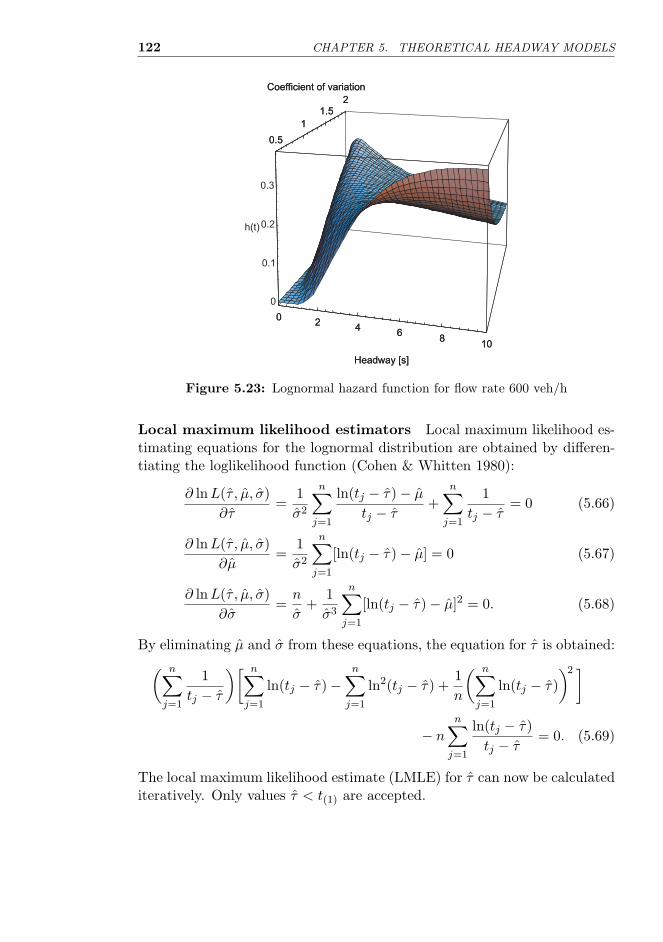
122 CHAPTER 5. THEORETICAL HEADWAY MODELS
02
46
810
Headway [s]
0.5
1
1.52
Coefficient of variation
0
0.1
0.2
0.3
h(t)
02
46
810
Headway [s]
0.5
1
1.52
Coefficient of variation
Figure 5.23: Lognormal hazard function for flow rate 600 veh/h
Local maximum likelihood estimators Local maximum likelihood es-timating equations for the lognormal distribution are obtained by differen-tiating the loglikelihood function (Cohen & Whitten 1980):
∂ lnL(τ , µ, σ)∂τ
=1σ2
n∑j=1
ln(tj − τ) − µ
tj − τ+
n∑j=1
1tj − τ
= 0 (5.66)
∂ lnL(τ , µ, σ)∂µ
=1σ2
n∑j=1
[ln(tj − τ) − µ] = 0 (5.67)
∂ lnL(τ , µ, σ)∂σ
=n
σ+
1σ3
n∑j=1
[ln(tj − τ) − µ]2 = 0. (5.68)
By eliminating µ and σ from these equations, the equation for τ is obtained:( n∑j=1
1tj − τ
)[ n∑j=1
ln(tj − τ) −n∑
j=1
ln2(tj − τ) +1n
( n∑j=1
ln(tj − τ))2 ]
− n
n∑j=1
ln(tj − τ)tj − τ
= 0. (5.69)
The local maximum likelihood estimate (LMLE) for τ can now be calculatediteratively. Only values τ < t(1) are accepted.

5.2. Simple Distributions 123
After τ has been solved, the scale and shape3 parameters can be esti-mated as follows (Cohen & Whitten 1980):
µ =1n
n∑j=1
ln(tj − τ) (5.70)
σ2 =1n
n∑j=1
ln2(tj − τ) −(
1n
n∑j=1
ln(tj − τ))2
. (5.71)
Although the LMLEs gave the best estimates of all the methods exam-ined, the method had convergence problems—and a series of Monte Carlotests with 9,999 replications of 63 samples is very sensitive to convergenceproblems. As a result, the local maximum likelihood method was rejected.
Modified maximum likelihood estimators The local maximum like-lihood method can be modified as explained on page 34. Equation (5.66) isreplaced by:
F−1(
1n + 1
∣∣∣∣ τ , µ, σ
)= t(1). (5.72)
This can be expressed in terms of the inverse normal PDF:
Φ−1(
1n + 1
)=
ln(t(1) − τ) − µ
σ. (5.73)
Now the set of equations consists of equations (5.67) and (5.68), and theabove equation. By eliminating µ and σ from these equations, the estimatingequation for τ is obtained (Cohen & Whitten 1980):
ln(t(1) − τ) − 1n
n∑j=1
ln(tj − τ)
− Φ−1(
1n + 1
)[1n
n∑j=1
ln2(tj − τ) −(
1n
n∑j=1
ln(tj − τ))2 ] 1
2
= 0. (5.74)
This equation can be solved iteratively. The scale and shape parameterestimates follow from (5.70) and (5.71).
The moment estimators for the lognormal distribution have a large sam-pling error, and they are not uniquely determined. The modified moment
3For terminology see (Crow & Shimizu 1988).

124 CHAPTER 5. THEORETICAL HEADWAY MODELS
0 500 1 000 1 500
0.0
0.2
0.4
0.6
0.8
1.0
P(K-S)
50-70 km/h 80-100 km/h
0 500 1 000 1 500
0.0
0.2
0.4
0.6
0.8
1.0
P(A-D)
50-70 km/h 80-100 km/h
Figure 5.24: The nonparametric K-S and the parametric A-D goodness-of-fit testsfor the lognormal distribution
estimation of Cohen & Whitten (1980) was also applied. The estimateswere not as accurate as the modified maximum likelihood estimates. Thelocal maximum likelihood method gave the most accurate estimates, but itwas rejected because of convergence problems. In the goodness-of-fit testsbelow the parameters were estimated by the modified maximum likelihoodmethod.
Goodness-of-fit tests
The goodness-of-fit was tested using the parametric Anderson-Darling (A-D)test. For each sample 9,999 replications were generated and analyzed. Figure5.24 shows the test results. For comparison, the results of nonparametricKolmogorov-Smirnov (K-S) tests are also presented.
The results are better than for the exponential or the gamma distri-bution, but the combined probabilities are still practically zero (A–D test:1.80 · 10−114, K–S test: 1.84 · 10−36). The fit is better on low speed roads(A–D test: 1.78 · 10−15), but the hypothesis of lognormal vehicle headwaysshould be rejected.
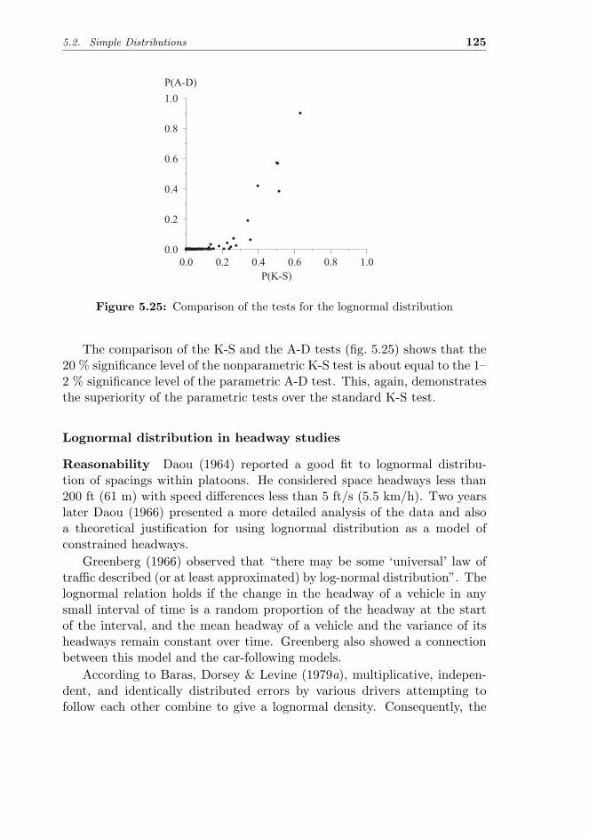
5.2. Simple Distributions 125
0.0 0.2 0.4 0.6 0.8 1.0
0.0
0.2
0.4
0.6
0.8
1.0
P(A-D)
Figure 5.25: Comparison of the tests for the lognormal distribution
The comparison of the K-S and the A-D tests (fig. 5.25) shows that the20 % significance level of the nonparametric K-S test is about equal to the 1–2 % significance level of the parametric A-D test. This, again, demonstratesthe superiority of the parametric tests over the standard K-S test.
Lognormal distribution in headway studies
Reasonability Daou (1964) reported a good fit to lognormal distribu-tion of spacings within platoons. He considered space headways less than200 ft (61 m) with speed differences less than 5 ft/s (5.5 km/h). Two yearslater Daou (1966) presented a more detailed analysis of the data and alsoa theoretical justification for using lognormal distribution as a model ofconstrained headways.
Greenberg (1966) observed that “there may be some ‘universal’ law oftraffic described (or at least approximated) by log-normal distribution”. Thelognormal relation holds if the change in the headway of a vehicle in anysmall interval of time is a random proportion of the headway at the startof the interval, and the mean headway of a vehicle and the variance of itsheadways remain constant over time. Greenberg also showed a connectionbetween this model and the car-following models.
According to Baras, Dorsey & Levine (1979a), multiplicative, indepen-dent, and identically distributed errors by various drivers attempting tofollow each other combine to give a lognormal density. Consequently, the

126 CHAPTER 5. THEORETICAL HEADWAY MODELS
lognormal distribution appears to be an attractive model for follower head-ways.
Applicability The modified maximum likelihood method requires rawheadway data and the application of numerical methods, but modified mo-ment estimates are relatively easy to calculate, although with some loss ofaccuracy. Lognormal random variate generation is relatively efficient withcurrently available routines. The lack of Laplace transform, however, limitsthe applicability of the lognormal distribution.
With currently available routines to calculate the PDF of the normaldistribution, even in pocket calculators, there is potential for a wider appli-cation of the lognormal distribution. In mathematical analysis the lognormaldistribution is more complicated than, say, the gamma distribution.
Validity Tolle (1971) studied the three parameter lognormal distributionfor headway data from a corridor on Interstate 71 in Ohio. The traffic vol-umes ranged from 800 to 1,900 veh/h. The location parameter was fixed(τ = 0.3). The K-S tests gave nonsignificant results in all samples at 5 %level. Six out of eleven samples produced nonsignificant values at 5 % sig-nificance level using the chi-square test. The results were best under lowestflow (800–1,200 veh/h) conditions. The significance probabilities were notpresented.
Branston (1976) studied headway data from M4 motorway in West Lon-don and from 50 sites on two-way roads around Bloomington, Indiana. Theresults of the chi-square tests4 for the 3-parameter lognormal distributionwere not very encouraging. Branston also used the lognormal distributionas a model for constrained headways in his lognormal generalized queuingmodel (see section 5.3.7).
As a statistical model for vehicle headways, the lognormal distributionhas two major problems (Luttinen 1994):
1. The goodness of fit, although better than for the exponential or thegamma distributions, is not acceptable.
2. The mathematical analysis presents some problems, because the log-normal distribution does not have a Laplace transform. If it is neces-
4Branston used average probability as a combined measure for goodness of fit. This,however, gives an unduly optimistic view. As an example: The five samples from the slowlane on M4 gave average probability 0.105, but the combined probability is 0.0002. Forthe mixed model, the 11 samples from loop 10 (Indiana) gave the best average probability0.327, but the combined probability is only 0.036.

5.3. Mixed distributions 127
sary to use numerical or Monte Carlo methods, one may as well use adistribution which fits the headway data better. Thus, the lognormaldistribution is neither simple enough nor realistic enough.
Consequently, the lognormal distribution has a limited use as an overallheadway distribution model, but it deserves proper attention in studies onfollower headways.
5.3 Mixed distributions
5.3.1 Structure of the model
The main problem of the simple distributions is their inability to describeboth the sharp peak and the long tail of the headway distribution. Evenat low volume conditions, there is a considerable accumulation of head-ways near the mode. Furthermore, the empirical hazard functions (figs. 4.6and 4.7, page 62) indicate that the tail is exponentially distributed. Theseproperties of the headway distributions suggest two vehicle categories—freeflowing and following. Because vehicles in different categories have differentheadway properties, the division should be included in the model, whichaccordingly becomes a mixture of two distributions.
According to Dawson & Chimini (1968) a vehicle is considered free, if:
1. The headway is of “adequate” duration.
2. The free vehicle is able to pass so that it does not have to modify itstime-space trajectory, as it approaches the preceding vehicle.
3. A passing vehicle has sustained a positive speed difference after thepassing maneuver so that the free vehicle is still able to operate as anindependent unit.
The other vehicles are followers. The vehicles could also be classified intofour or five categories:
1. Free flowing vehicles
2. Followers
3. Vehicles in a transition stage from free flowing to follower
4. Vehicles starting a passing maneuver.

128 CHAPTER 5. THEORETICAL HEADWAY MODELS
1-p
p
G
M
Figure 5.26: Queuing model for a mixed headway distribution
A fifth category would include the vehicles in the state of passing, but thesevehicles are driving on the other lane.
The vehicles with moderate headways are a mixture of categories 1, 2,3 and 4. Because it is difficult to make a distinction between vehicles incategories 2, 3 and 4, and in order to keep the model simple, the headwaydistribution is considered as a mixture of free headways and constrained(follower) headways only. A follower is then any vehicle in category 2, 3 or4.
The most common approach with two vehicle categories is to consider amixture of two probability distributions. A vehicle (X) is either a follower(X = 1) or a free flowing vehicle (X = 2). In terms of queuing theory, thismodel may be described as a system of two servers, only one of which mayserve at a time (fig. 5.26). There is a continuous queue of vehicles to thesystem. Each vehicle is served by server 1 with probability p and by server2 with probability 1 − p. Server i has service time distribution fi(t). Theheadway distribution model is the distribution of departure intervals fromthe system. This system differs from an ordinary queuing system in tworespects:
1. The system is always busy because of a continuous queue to the system.
2. Only one customer (vehicle) may be in the system at a time.
The model may be analyzed by the methods of the queuing theory, andespecially by the method of stages (Cooper 1981, Luttinen 1990).

5.3. Mixed distributions 129
5.3.2 Properties of the model
The density functions for constrained headways [f1(t)] and free headways[f2(t)] are the conditional densities:
f1(t) = f( t |X = 1 ) (5.75)f2(t) = f( t |X = 2 ) . (5.76)
If the proportion of constrained headways is p, the probability density func-tion (pdf) of the headway distribution is:
f(t) = pf1(t) + (1 − p)f2(t). (5.77)
The hazard function is:
h(t) =f(t)
1 − F (t)=
pf1(t) + (1 − p)f2(t)1 − [pF1(t) + (1 − p)F2(t)]
. (5.78)
The distribution has Laplace transform:
f∗(s) = pf∗1 (s) + (1 − p)f∗
2 (s) (5.79)
where f∗i (s) is the transform of fi(t), if the transform exists.
The mean is:
µ(T ) = pµ(T1) + (1 − p)µ(T2). (5.80)
where µ(Ti) is the expectation of headway variate Ti from distribution fi(t).Higher noncentral moments are obtained similarly:5
E(T r) = pE(T r1 ) + (1 − p)E(T r
2 ). (5.81)
Variance, skewness and kurtosis can be calculated using the relations be-
5 The moments can also be obtained by using the derivatives of the Laplace transform:
E(T r) = (−1)r drf∗(s)dsr
∣∣∣∣s=0
.

130 CHAPTER 5. THEORETICAL HEADWAY MODELS
tween central and noncentral moments:
σ2(T ) = E[T − µ(T )]2 (5.82)
= E(T 2) − [µ(T )]2
α3(T ) =E[T − µ(T )]3
σ3(T )(5.83)
=1
σ3(T ){E(T 3) − 3µ(T )E(T 2) + 2[µ(T )]3
}α4(T ) =
E[T − µ(T )]4
σ4(T )(5.84)
=1
σ4(T ){E(T 4) − 4µ(T )E(T 3) + 6[µ(T )]2E(T 2) − 3[µ(T )]4
}.
Some proposed mixed distribution models are presented below. Detailedanalysis and goodness-of-fit tests for all these distributions are beyond thescope of this research. The semi-Poisson distribution is given considerableattention, but other mixed distributions are discussed more briefly, usingonly information that has been readily available. Because all the models arebased on the assumption of exponentially distributed large headways, theexponential tail hypothesis is examined first.
5.3.3 The exponential tail hypothesis
Goodness-of-fit tests
The exponential tail hypothesis states that headways greater than a thresh-old (δ) follow the negative exponential distribution:
H0 : 1 − Fn(t) ∼ e−θt, t > δ, (5.85)
where θ is the scale parameter estimate and n is the number of headwaysgreater than δ in the sample. The test has two stages:
1. Determination of δ
2. Goodness-of-fit test for headways greater than δ.
The goodness-of-fit tests were conducted using threshold values 0–14.5 inincrements of 0.5. Parametric Monte Carlo tests with the A-D statistic wereused. The number of replications was 9,999. The significance probabilitieswere combined using the method described in section 2.2.5 (page 43).

5.3. Mixed distributions 131
0 2 4 6 8 10 12 14
0.0
0.2
0.4
0.6
0.8
1.0
Significance
Volume [veh/h]
0-500
500-1000
> 1000
Figure 5.27: Goodness-of-fit tests for the exponential tail (50–70 km/h)
Figures 5.27 and 5.28 show the combined significance probabilities fordifferent volume levels. Figure 5.29 shows the combined significance prob-abilities for different speed limits. The threshold value for the exponentialtail hypothesis is eight seconds, after which the test results are nonsignif-icant. Because of such a large threshold value, a positively skew headwaydistribution should be considered for the follower headways.
Low speed roads (fig. 5.27 and 5.29) show nonsignificant values also at4.5 ≤ δ ≤ 6 s. This phenomenon appears at all volume levels. It may indi-cate lower threshold values. The lower threshold (δ = 4.5) is, however, notaccepted, because there are significant deviations from the exponential dis-tribution at (4.5s < δ < 8s). The speed difference data (fig. 5.30, page 133)also support a higher threshold.
Miller (1961) tested for threshold values four, five and six seconds, andfound δ = 6 s about ideal. His data were from a straight section on a two-lane road between Stockholm and Uppsala in Sweden. He noted that thereis a slight excess of observed intervals in the 6–8 s range as some driversbegin to slow down, when they approach this close to the vehicle ahead. Hedecided that some criterion based upon relative velocities is necessary fordetermining the platoons, when time intervals are less than eight seconds.
Wasielewski (1979) studied the exponential tail hypothesis of headwaydistributions from the center westbound lane of Route I-94, a six-lane di-vided urban expressway in Detroit. He found no significant deviations fromthe exponential distribution, when the threshold was 2.5 seconds for volumes

132 CHAPTER 5. THEORETICAL HEADWAY MODELS
0 2 4 6 8 10 12 14
0.0
0.2
0.4
0.6
0.8
1.0
Significance
Volume [veh/h]
0-500
500-1000
> 1000
Figure 5.28: Goodness-of-fit tests for the exponential tail (80–100 km/h)
0 2 4 6 8 10 12 14
0.0
0.2
0.4
0.6
0.8
1.0
Significance
Speed limit [km/h]
50-70
80-100
50-100
Figure 5.29: Goodness-of-fit tests for the exponential tail

5.3. Mixed distributions 133
0 5 10 15 20
0
2
4
6
8
10
12
14
16
Standard deviation of relative speeds
Speed limit
50-70 km/h
80-100 km/h
Figure 5.30: Standard deviation of speed differences
less than 1,450 veh/h and 3.5 seconds for volumes greater than 1,450 veh/h.These values are too low for two-lane roads.
It is possible that the goodness-of-fit tests give too small threshold es-timates. The tests cannot detect small deviations from the exponentialdistribution for headways slightly greater than δ, if the tail is exponential.Consequently, an alternative approach was also examined.
Speed differences
Properties of speed differences Car-following models (section 2.1) sug-gest that the speed difference (relative speed) between the leader and thefollower (vi−1−vi) is a decisive factor in the car-following process. A followeradjusts the speed of the vehicle to the speed of the leading vehicle. Thisspeed adjustment decreases the variation of speeds among trailing vehicles.At some time distance the interaction of speeds vanishes.
Figure 5.30 shows the standard deviation (sυ) of speed differences ofconsecutive vehicles against the headway. Headways are combined in onesecond intervals (t−1,t]. At short headways (1–5 s) sυ is small and increasesas the headway increases. At large headways (t > 10 s) sυ is rather constant.On high speed roads sυ is larger than on low speed roads.
A piecewise linear model was fitted to the data—rising slope for head-ways less than the threshold and a constant value for headways greater thanthe threshold. The sυ’s were weighted by the number of observations in theinterval. On both low and high speed roads the threshold value of about 9 s

134 CHAPTER 5. THEORETICAL HEADWAY MODELS
was obtained. However, more extensive data sets and more accurate mea-suring equipment are needed for further analysis, because speed differenceshave larger measurement errors than absolute speeds.
This result is in agreement with the goodness-of-fit tests above. Theoriginal Bureau of Public Roads (1950) reports a similar analysis and virtu-ally the same result. Chishaki & Tamura (1984) present a very similar figureof the variance of the speed differences. Branston (1979) reports thresholdvalues 4.5 s and 3.75 s for the nearside and offside lanes on M4 motorwayin West London.
Enberg & Pursula (1992) have shown that on high-class two-lane ruralroads, the relation between the headways and the standard deviation ofspeed differences is similar to figure 5.30. For headways larger than aboutfive seconds, there is no significant increase in the standard deviation. Whenthe headway is less than one second, the standard deviation jumps to about10 km/h. This phenomenon is also reported in Bureau of Public Roads(1950) and by Branston (1979). A similar, but not as strong, phenomenoncan be seen on high speed roads in figure 5.30. It may be assumed, that atvery short headways some vehicles are starting to pass the vehicle ahead.The increase in sυ is very small or nonexistent in figure 5.30, because therewere only few passing vehicles.
Figure 5.30 shows that vehicles may be divided into three categories.Leading vehicles are not affected by vehicles ahead. The drivers select theirown desired speed and headways can be assumed to follow the exponen-tial distribution. Trailing vehicles follow the vehicle ahead and adjust theirspeeds accordingly. Because the mode of the headway distribution is about1.5 seconds, this headway can be assumed to be the average desired head-way of the followers. In addition to these two classes there are vehicles ina transition stage. These vehicles are neither following the vehicle aheadnor driving freely. The transition stage seems to begin, when the headwayis about 8–9 seconds. Speed adjustment decreases the variation betweenspeeds of consecutive vehicles. At headways less than one second, the speedvariation increases again on high speed roads, because the vehicles startingto pass have greater speed than the vehicle ahead.
Figures 5.31 and 5.32 show some basic statistics of speed difference distri-butions. Mean is near zero at all headways. As the headway is between twoand eight seconds, the mean is slightly positive, which is probably causedby passers that have returned to the right lane. For headways greater thaneight seconds the variation in the mean increases, and the mean oscillatesaround zero. When the headways are greater than ten seconds, the meanspeed difference is negative. In this case some proportion of the vehicles

5.3. Mixed distributions 135
0 2 4 6 8 10 12 14
-4
-2
0
2
4
6
8
10
12 Mean
Skewness
Kurtosis
Figure 5.31: Mean, skewness and kurtosis of speed difference distributions (50–70 km/h)
ahead are followers having constrained speeds (vi−1), while the speeds ofthe vehicles behind (vi) are nonconstrained.
The skewness indicates that the speed difference distribution is practi-cally symmetric. On high speed roads at headways less than one second, theskewness has a rather large negative value. Considering the slightly negativemean and the increased standard deviation, the negative skewness is mostlikely caused by vehicles beginning to pass, thus producing negative speeddifferences.
Summala & Vierimaa (1980) found that the speed difference distributionbecomes skew, as the spacing grows over 50 m. At spacings longer than200 m the distribution is again symmetric. This phenomenon is not foundin figures 5.31 and 5.32.
The most significant feature in the figures is the excessively positivekurtosis at short headways. (The kurtosis is scaled so that the normal dis-tribution has null kurtosis.) The speed difference distributions are moresharply peaked than the normal distribution (see also fig. 5.33). This istrue especially for headways less than four seconds. The kurtosis is largestat headways between one and two seconds, and the peak is higher on highspeed roads. Because at headways between one and two seconds the distri-bution is symmetric with zero mean, it is evident that at these headwaysmost drivers are content to follow the leader at the same speed. The kurto-sis approaches zero and the distribution approaches normality at headways

136 CHAPTER 5. THEORETICAL HEADWAY MODELS
0 2 4 6 8 10 12 14
-4
-2
0
2
4
6
8
10
12 Mean
Skewness
Kurtosis
Figure 5.32: Mean, skewness and kurtosis of speed difference distributions (80–100 km/h)
larger than seven seconds on low speed roads, and at headways larger thanten seconds on high speed roads. The variation in the kurtosis increases atlarge headways due to fewer observations.
Proportion of free headways The distribution of speed differences atlong headways can be assumed to be the distribution of speed differences forfree flowing vehicles. The mean and standard deviation of speed differencesat headways t ≥ 10 s are υ = −0.879 and sυ = 10.492 on low speed roads,and υ = −0.862 and sυ = 11.660 on high speed roads. Assuming normality,the means do not differ significantly from zero, but the nonequality of thestandard deviations is statistically significant (at level P = 0.001). On highspeed roads the speed differences have larger variation.
Because not every vehicle having a headway shorter than eight secondsis a follower, the distribution of their speed differences is a mixture of freespeed differences and constrained speed differences. If the speed differencedistribution f2(µ1, σ2) of free flowing vehicles is estimated, the speed differ-ence distribution f(µ, σ) of all vehicles can be estimated as a mixed normaldistribution (fig. 5.30):
f(µ, σ) = pf1(µ1, σ1) + (1 − p)f2(µ2, σ2), (5.86)
The proportion of trailing vehicles (p) and the parameters of the speeddifference distribution (µ1, σ1) of trailing vehicles must be estimated fromthe data.

5.3. Mixed distributions 137
-18 -12 -6 0 6 12 180.00
0.05
0.10
0.15
0.20
0.25
0.30
Frequency
Observed
Trailing
All
Free
Figure 5.33: Mixed normal distribution for speed differences on high speed (80–100 km/h) roads
The minimum chi-square method (section 2.2.3) was used to estimate p,while maximum likelihood estimates were used for µ1 and σ1. The estimatefor the proportion of free flowing vehicles (1 − p) among headways t ≤ 8 sis 20 % on high speed roads and 15 % on low speed roads. The proportionof trailing vehicles is approximately the same as the proportion of headwayst ≤ 3 s on high speed roads and t ≤ 5 s on low speed roads.
Parameter estimation for the exponential tail
The goodness-of-fit tests above (p. 130) indicated that headways larger thaneight seconds belong to the exponential tail. Assuming the eight secondthreshold, the scale parameter estimate for the exponential tail is equal tothe scale parameter estimate for the shifted exponential distribution withτ = 8 s:
θ =1
t8 − 8(5.87)
where t8 is the mean of headways greater than eight seconds.The number of free vehicles can be assumed to increase with increasing
flow rate. Consequently, the scale parameter (θ) of the exponential tail canbe assumed to have a positive correlation with the traffic volume (λ).6 Alinear model (θ = a + bλ) was tested using the linear regression analysis.
6See also section 4.2.3, page 60.

138 CHAPTER 5. THEORETICAL HEADWAY MODELS
0 500 1 000 1 500
0.0
0.1
0.2
0.3
0.4
0.5
0.6
0.7
Scale parameter
Speed limit
50-70 km/h
80-100 km/h
Figure 5.34: Scale parameter estimates for the exponential tail
Because the analysis of covariance (ANCOVA) indicated that there is asignificant (P = 0.006) difference between the scale parameter estimates forlow speed and high speed roads, separate models (θ50, θ80) were tested forboth road categories. The constant term (a) was omitted, because it did notdiffer significantly from zero. (As the flow rate approaches zero, the scaleparameter must also approach zero.) The following equations for the scaleparameter estimates were obtained (fig. 5.34):
θ50 = 0.813λ (5.88)
θ80 = 0.561λ, (5.89)
where λ is the traffic volume [veh/s].7
In order to stabilize the variance, which increases with growing trafficvolume, 1/λ2 was used as a weighting factor. The coefficient of determina-tion is R2 = 0.936 for low speed roads and R2 = 0.823 for high speed roads.The significance of the regression is P < 0.0005 in both cases.
On high speed roads the estimates are lower. This indicates a “longertail” and accordingly higher coefficient of variation, skewness and kurtosis.The scale parameter estimates are also the estimates for the hazard rate atthe tail of the headway distribution.
7Wasielewski (1979) obtained for a center expressway lane:
θ = −0.058 + 1.401λ. (5.90)

5.3. Mixed distributions 139
The scale parameter was estimated using the location parameter valueof eight seconds. The estimate is, however, valid even if the true locationparameter has a lower value. This can be shown easily. If the true locationparameter is a, then:
P{T > t} = e−θ(t−a). (5.91)
If only headways greater than b (and a < b) are examined, then:
P{ T > t |T > b } =e−θ(t−a)
e−θ(b−a)
= e−θ(t−b).
(5.92)
A larger location parameter does not cause any bias in the scale parame-ter estimate. The estimate is, however, based on fewer observations, thusreducing the accuracy.
5.3.4 Hyperexponential distribution
Properties of the hyperexponential distribution
Hyperexponential distribution was first applied to headway studies bySchuhl (1955), hence it is also known as Schuhl’s (composite exponential)distribution. If both leader and follower headways are exponential, the head-way distribution is:
f( t | p, θ1, θ2 ) = pθ1e−θ1t + (1 − p)θ2e
−θ2t. (5.93)
The headways are produced by a service system with two parallel servers,each having exponential service times (fig. 5.35). As noted above, there is aconstant queue to the system.
The pdf of the hyperexponential distribution (fig. 5.36) starts fromf(0) = pθ1 + (1 − p)θ2 and decreases asymptotically to zero. The hazardfunction decreases from h(0) = pθ1 +(1−p)θ2 to limt→∞ h(t) = min {θ1, θ2}(Trivedi 1982). The coefficient of variation is C(T ) ≥ 1 (Trivedi 1982).
Schuhl (1955) used a location parameter (τ) for the follower headways.The resulting pdf was:
f( t | p, τ, θ1, θ2 ) = pθ1e−θ1(t−τ) + (1 − p)θ2e
−θ2t. (5.94)
Free headways were not given a location parameter, because these vehicleswere considered free to pass.

140 CHAPTER 5. THEORETICAL HEADWAY MODELS
1-p
p
M
M
1
2
Figure 5.35: Queuing model for the hyperexponential distribution
02
4 6 8 10
Headway [s]
200400
600800
Volume [veh/h]
0
0.1
0.2
0.3
f(t)
02
4 6 8 10
Headway [s]
200400
600800
Volume [veh/h]
Figure 5.36: Hyperexponential density functions with parameters by Grecco &Sword (1968)

5.3. Mixed distributions 141
Hyperexponential distribution in headway studies
Reasonability As compared with the negative exponential and the shiftedexponential distributions, the hyperexponential distribution has the advan-tage of being able to produce a larger coefficient of variation. It also hasseparate models for free and follower headways. The negative exponentialdistribution is, however, not an appropriate model for constrained headways.The problem of too short headways can be avoided by location parameters,but this introduces an artificial discontinuity in the density function.
Applicability Pseudo-random number generation is fast, although not asefficient as for the negative exponential distribution. The Laplace transformhas a simple form:
f∗( s | p, θ1, θ2 ) = pθ1
s + θ1+ (1 − p)
θ2
s + θ2. (5.95)
Without location parameters the hyperexponential distribution has threeparameters to estimate. Introducing one or two location parameters in-creases the total number of parameters to four or five, which makes theparameter estimation more difficult.
Grecco & Sword (1968) assumed a fixed value of τ = 1 s for the locationparameter, and estimated the three remaining parameters by minimizingthe chi-square statistic. The regression equations for the parameters were:
p =0.115λ
100(5.96)
τ = 1 (5.97)
θ1 = 0.4 (5.98)
θ2 =1
24 − 0.0122λ, (5.99)
where λ is the traffic volume [veh/h]. These estimates are, however, validonly for λ < 870 veh/h, since p > 1 for λ ≥ 870 veh/h. Figure 5.36 showsthe pdf calculated with these parameter values.
Griffiths & Hunt (1991) applied the location parameter (τ) to both f1(t)and f2(t), and called the model double displaced negative exponential distri-bution (DDNED). The parameters were estimated by a “hybrid method”,using the equations for the mean and the variance as constraints, and min-imizing the chi-square statistic. The estimation was constrained so that p

142 CHAPTER 5. THEORETICAL HEADWAY MODELS
remained in the range 0 < p ≤ 0.5, and τ was required to be greater [sic]8
than the smallest observed headway (t(1)).
Validity Grecco & Sword (1968) collected headway data on a two-laneportion of the U.S. 52 bypass. The headway data were grouped in onesecond intervals up to twenty seconds. The data were collected in volumegroups using the class length of 100 veh/h. The chi-square tests with 8–17degrees of freedom gave acceptable fit for volumes less than 700 veh/h. Thecombined probability (calculated by the present author) of the six tests is0.79.
Griffiths & Hunt (1991) examined the vehicle headways in urban areas.The model had the same location parameter τ for both f1(t) and f2(t).The mean of τ was 1.5 s, the minimum 0.58 s, and the maximum 2.66 s.The chi-square test with 5 % significance level gave acceptable fit for 78 of86 data sets. Because τ was greater than the shortest observed headway ineach sample, the model would have failed all A-D tests with null significancelevel.
Sainio (1984) tested the hyperexponential distribution9 against headwaydata from high class Finnish highways. He presented only the chi-squaretest statistic values for the five samples. When the significance probabilitiesare calculated (ν = 10), the model is rejected in three samples at 0.01 level.The combined significance probability is 3.9 · 10−6.
The hyperexponential distribution does not pass the identification pro-cess. Although the coefficient of variation can be greater than unity, theshape of the pdf and the hazard function do not have the correct shape.The hyperexponential distribution has similar properties as the gamma dis-tribution with shape parameter less than unity. The pdf has a similar shape,and the c.v. is larger than unity. The hyperexponential distribution, how-ever, has a more reasonable hazard rate at t = τ , and the kurtosis is slightlycloser to the empirical kurtosis, when plotted against the squared skewness.Consequently, the identification process suggests that the hyperexponentialdistribution could perform slightly better than the gamma distribution as aheadway model.
8If the location parameter (τ) is greater than the smallest headway (t(1)), the proba-bility P
{T ≤ t(1)
}is null. Consequently, the headway sample cannot be generated by the
proposed model.9Sainio (1984) called it the Kell distribution (see Kell 1962).

5.3. Mixed distributions 143
p
1-p
M 1 M 1
M 2
D 1
D 2
Figure 5.37: Queuing model for the hyperlang distribution
5.3.5 Hyperlang distribution
Properties of the hyperlang distribution
Dawson (in Drew 1967, Dawson & Chimini 1968, Dawson 1969) has sug-gested the Erlang-distribution as a model for constrained headways. Theheadways in the hyperlang (hyper-Erlang) model are produced by a servicesystem with two alternative channels (fig. 5.37). Channel 1 is selected withprobability p, and it has one server with Erlang-distributed service times,or alternatively r servers in series each having the same exponential servicetime distribution. The service time distribution in channel 2 is exponential.A location (threshold) parameter is shown as a server (D) with a constantservice time.
The hyperexponential distribution is naturally a special case of the hyp-erlang distribution (r = 1). The generalization to exponential-gamma mix-ture distribution is straightforward.
The pdf of the hyperlang distribution is:10
f( t | p, τ1, θ1, τ2, θ2, r ) = pθr1(t − τ1)r−1
(r − 1)!e−θ1(t−τ1) + (1 − p)θ2e
−θ2(t−τ2).
(5.100)
10In place of θi Dawson (1969) used parameter γi, so that:
θi =1
γi − τi,
where γi is the average headway in channel i.

144 CHAPTER 5. THEORETICAL HEADWAY MODELS
The distribution has Laplace transform (Luttinen 1990):
f∗( s | p, τ1, θ1, τ2, θ2, r ) = p
(θ1
s + θ1
)r
e−sτ1 + (1 − p)θ2
s + θ2e−sτ2 . (5.101)
The mean and the variance are (Luttinen 1990):
µ(T ) = p
(1θ1
+ τ1
)+ (1 − p)
(r
θ2+ τ2
)(5.102)
σ2(T ) = p
[(1θ1
+ τ1
)2
+1θ1
]+ (1 − p)
[(r
θ2+ τ2
)2
+r
θ2
](5.103)
−[p
(1θ1
+ τ1
)+ (1 − p)
(r
θ2+ τ2
)]2.
The hazard function of the hyperlang distribution is similar to the empir-ical hazard function, except that at zero headway h( 0 | p, θ1, θ2, r ) = θ2,assuming τ1 = τ2 = 0 (Trivedi 1982).
Hyperlang distribution in headway studies
Reasonability The hyperlang distribution has exponential tail, and theshape of the pdf is similar to the empirical headway distributions. Someadditional flexibility could be obtained using gamma distribution for con-strained headways.
The distribution avoids extremely short headways, but the location pa-rameter (τ2) of the free headway distribution makes the pdf and the hazardfunction discontinuous. The model assumes that the frequency of free head-ways is highest, when the headway is only slightly greater than τ2, and thereare no free headways, when t is a little smaller than τ2. The problem is moreoutstanding at low flow conditions, when the proportion of free headways islarge.
Applicability The large number of parameters (six) causes problems inparameter estimation. Dawson & Chimini (1968) and Summala & Vierimaa(1980) have estimated the parameters using least squares fit. For the head-way data in HCM (1965), Dawson & Chimini (1968) estimated r = 2 andτ2 = 0.75 for all samples. The estimated density and hazard functions aredisplayed in figures 5.38 and 5.39.
The generation of pseudorandom numbers is reasonably effective. TheLaplace transform exists, but the mathematical analysis is more tediousthan the analysis of the exponential and the gamma distributions.

5.3. Mixed distributions 145
02
4 6 8 10
Headway [s]
150450
7501050
Volume [veh/h]
0
0.05
0.1
0.15
f(t)
02
4 6 8 10
Headway [s]
150450
7501050
Volume [veh/h]
Figure 5.38: Hyperlang density functions [parameters by Dawson & Chimini(1968)]
02
46
810
Headway [s]
150
450
7501050
Volume [veh/h]
0
0.1
0.2
0.3
h(t)
02
46
810
Headway [s]
150
450
7501050
Volume [veh/h]
Figure 5.39: Hyperlang hazard functions [parameters by Dawson & Chimini(1968)]

146 CHAPTER 5. THEORETICAL HEADWAY MODELS
M
Figure 5.40: M/D/1 queuing model
Validity Dawson & Chimini (1968) and Dawson (1969) did not report anygoodness-of-fit tests. Because the hyperlang distribution is a generalizationof negative exponential, shifted exponential, Erlang and hyperexponentialdistributions, it is likely to fit the headway data better. But for a six pa-rameter distribution, the goodness-of-fit requirements are extremely high.
5.3.6 M/D/1 queuing model
Tanner (1953, 1961) has modeled the arrival process as a M/D/1 queuingprocess (fig. 5.40). The service system has one server with constant servicetime (τ). There is not, however, a continuous queue to the service point,but the arrival process is Poisson.
The vehicles in platoons have constant headways, and the free headwaysfollow the shifted exponential distribution. The probability for a followerheadway (t = τ) is equal to the utilization factor11 (ρ) of the server:
P{T = τ} = λτ = ρ (5.104)
For steady state conditions, the utilization factor must be less than unity.The platoon length follows the Borel distribution, and the probability forplatoon length k is (Tanner 1961):
pk =(λτk)k−1
n!e−λτk. (5.105)
Because the platoon length distribution is not geometric, the headways arenot i.i.d.
11The utilization factor (ρ) is the expected number of arrivals per mean service timein the limit (Gross & Harris 1985), or equivalently the fraction of time that the server isbusy (Kleinrock 1975).

5.3. Mixed distributions 147
02
4 6 8 10
Headway [s]
200600
10001400
Volume [veh/h]
0
0.05
0.1
0.15
0.2
f(t)
02
4 6 8 10
Headway [s]
200600
10001400
Volume [veh/h]
Figure 5.41: M/D/1 density function (τ = 1 s)
The PDF of departure intervals (headways) is discontinuous (Luttinen1990):
F( t |λ, τ ) =
{0, if t < τ
1 − (1 − λτ)e−λ(t−τ), otherwise.(5.106)
The pdf is obtained by differentiation (Luttinen 1990):
f( t |λ, τ ) =
{0, if t < τ
(1 − λτ)λe−λ(t−τ), otherwise.(5.107)
The pdf is equal to the pdf of the shifted exponential distribution multipliedby the server idleness factor (1 − ρ). The mean, the variance, and thecoefficient of variation are (Luttinen 1990):
µ(T ) =1λ
(5.108)
σ2(T ) =1λ2 − τ2 (5.109)
C(T ) =√
1 − λ2τ2 ≤ 1. (5.110)
Cowan (1975, 1978), used the headway distribution assuming a renewalprocess. The Cowan M3 model is accordingly a generalization of the M/D/1

148 CHAPTER 5. THEORETICAL HEADWAY MODELS
model:
F( t | θ, λ ) =
{0, if t < τ
1 − (1 − θ)e−λ(t−τ), otherwise.(5.111)
The parameters of the M/D/1 headway model can be easily estimatedby the method of moments. The scale parameter estimate (λ) is equal tothe traffic volume:
λ =1t, (5.112)
and it does not depend on τ . The trailing headway (τ) can be estimatedusing the sample variance:
τ =√
1λ2
− s2 (5.113)
M/D/1 queuing model in headway studies
Reasonability In some sense the M/D/1 model follows logically from theshifted exponential distribution: If the vehicles move freely at headwaysgreater than τ , and headways shorter than τ are not possible, there mustbe some platooning with headways equal to τ . The model separates leadingand following vehicles, but the hypothesis of constant headways for followingvehicles is unrealistic.
Applicability The M/D/1 model is rather simple to analyze mathemat-ically. The parameter estimation is straightforward, and the generation ofpseudorandom variates does not present any problems.
Validity Sullivan & Troutbeck (1994) applied the Cowan’s M3 model tourban traffic flow. They concluded that the model is appropriate to eval-uate the performance of roundabouts and unsignalized intersections, whereaccuracy is only required for headways greater than the critical gap. Theydid not present any goodness-of-fit tests.
Akcelik & Chung (1994) described the calibration of the M3 model,which they called the “bunched exponential distribution”. On the basis ofvisual evaluation they considered that the model provides good estimatesof arrival headways, and they strongly recommended its use in stead of thenegative exponential and the shifted exponential distributions.

5.3. Mixed distributions 149
02
4 6 8 10
Headway [s]
200600
10001400
Volume [veh/h]
0
0.1
0.2
0.3
h(t)
02
4 6 8 10
Headway [s]
200600
10001400
Volume [veh/h]
Figure 5.42: M/D/1 hazard function (τ = 1 s)
The discontinuity of the pdf and even the PDF is a major problem inthe model. The goodness-of-fit becomes worse as the proportion of trailingvehicles (ρ) increases. The unfeasibility of the model is, however, mostobvious in the hazard function plot of figure 5.42. In addition, the coefficientof variation is too low for most flow conditions.
5.3.7 Generalized queuing model
A queuing model with Poisson arrivals and a general service time distribu-tion (fig. 5.43) is called the M/G/1 queuing system (fig. 5.43). It producesfollower headways (T1) as long as the server is busy. With probability 1−p,the server experiences some idleness during the interdeparture period. Thelength of an interdeparture time with idleness is the sum of the service time(T1) and the idle time (T2) (Gross & Harris 1985). The density of this sumis the convolution (f1 ∗ f2) of the service time density and the interarrivaltime density, where interarrival time density (f2) is exponential.
The pdf of the interdeparture time distribution is:
f(t) = pf1(t) + (1 − p)∫ t
0f1(u)θe−θ(t−u)du
= pf1(t) + (1 − p)θe−θt
∫ t
0f1(u)eθudu.
(5.114)

150 CHAPTER 5. THEORETICAL HEADWAY MODELS
M
Figure 5.43: M/G/1 queuing system
The PDF is (Gross & Harris 1985):
F (t) = pF1(t) + (1 − p)∫ t
0F1(t − u)θe−θudu, (5.115)
or equivalently:
F (t) = pF1(t) + (1 − p)∫ t
0f1(u)
(1 − e−θ(t−u)
)du
= F1(t) − (1 − p)e−θt
∫ t
0f1(u)eθudu.
(5.116)
The Laplace transform is obtained using the convolution property12 of thetransform:
f∗(s) = pf∗1 (s) + (1 − p)f∗
1 (s)f∗2 (s)
= pf∗1 (s) + (1 − p)f∗
1 (s)θ
s + θ.
(5.117)
The proportion of interdeparture times with no idleness (p) is equal to theutilization factor (ρ) of the server (Gross & Harris 1985):
ρ =µ(T1)µ(T2)
. (5.118)
Cowan (1975) used gamma distributed service times. Branston (1976)applied both gamma and lognormal service time distributions. The modelswere modified so that p was not equal to the utilization factor, but it wasestimated from the data. Cowan called this model M4, while Branston calledit the generalized queuing model. Figure 5.44 shows the pdf of the model withlognormal follower headways. The parameters follow the approximationsgiven by Branston. Figure 5.44 shows the corresponding hazard function.

5.3. Mixed distributions 151
0 2 4 6 8 100.0
0.1
0.2
0.3
0.4
Density
Follower headway component
Free headway component
Headway pdf Parameters:
p = 0.437
µ = 0.304
σ = 0.450
θ = 0.196
Figure 5.44: Density function of the lognormal generalized queuing model
0 2 4 6 8 100.0
0.1
0.2
0.3
0.4
0.5
Hazard rate
Parameters:
p = 0.437
µ = 0.304
σ = 0.450
θ = 0.196
Figure 5.45: Hazard function of the lognormal generalized queuing model

152 CHAPTER 5. THEORETICAL HEADWAY MODELS
For comparison with the semi-Poisson distribution, some properties ofthe generalized queuing model with gamma distributed service times arepresented. The pdf is:13
f( t | p, β, α, θ ) = pβαtα−1
Γ(α)e−βt + (1 − p)
βα
Γ(α)θe−θt
∫ t
0uα−1e−u(β−θ)du
= pβαtα−1
Γ(α)e−βt
+ (1 − p)(
β
β − θ
)α γ[α, t(β − θ)]Γ(α)
θe−θt,
(5.119)
where γ(·) is the incomplete gamma function (see table 5.3, page 104). Thepdf may also be expressed as:
f( t | p, β, α, θ ) = pf1( t | β, α )
+ (1 − p)(
β
β − θ
)α
F1( t | β − θ, α )f2( t | θ ). (5.120)
Correspondingly, the PDF can be expressed as:
F ( t | p, β, α, θ ) =γ(α, βt)
Γ(α)− (1 − p)
(β
β − θ
)α γ[α, t(β − θ)]Γ(α)
e−θt
= F1( t | β, α ) − (1 − p)(
β
β − θ
)α
F1( t | β − θ, α )[1 − F2( t | θ )]. (5.121)
The Laplace transform is:
f∗(s) =(
β
s + β
)α(p + (1 − p)
θ
s + θ
). (5.122)
The moments as well as the measures of variation, skewness and kurtosis
12Convolution property of the Laplace transform:
f∗X+Y = f∗
Xf∗Y .
See Kleinrock (1975).13See relation 3.381.1 in Gradshteyn & Ryzhik (1980).

5.3. Mixed distributions 153
are now easily obtained:
µ(T ) =α
β+
1 − p
θ(5.123)
σ2(T ) =α
β2 +1 − p2
θ2 (5.124)
C(T ) =
√αθ2 + β2(1 − p2)αθ + β(1 − p)
(5.125)
α3(T ) =2[β3(1 − p3) + αθ3]
[β2(1 − p2) + αθ2]3/2 (5.126)
α4(T ) =3{β4[4 − (1 + p2)2
]+ αθ2[2β2(1 − p2) + θ2(α + 2)]
}[β2(1 − p2) + αθ2]2
. (5.127)
Three special cases are worth mentioning:
1. p = 1. The model is equal to the gamma distribution [µ(T ) = α/β].
2. p = 0. The headway distribution is the sum of a gamma and an ex-ponential random variate [µ(T ) = α/β + 1/θ]. As the mean followerheadway (α/β) approaches null, the distribution of all headways ap-proaches exponentiality [µ(T ) = 1/θ].
3. p = ρ < 1. The departure rate is equal to the arrival rate [1/µ(T ) = θ].This is the M/G/1 model.
Generalized queuing model in headway studies
Reasonability According to Cowan (1975) the generalized queuing modeldescribes a situation that an ∞-lane road merges into one lane accordingto the first-come–first-merge rule such that each driver leaves a randomlychosen tracking headway. The headways at the entry point can be describedby the generalized queuing model.
Wasielewski (1979) criticizes the generalized queuing model for lackingin a physical basis. A free headway is a sum of a constrained headway (T1)and an exponential variate (T2). But the rationale for selecting exponentialdistribution for free headways lies in the fact that these vehicles are notinfluenced by the vehicle ahead.
Wasielewski prefers the semi-Poisson distribution, but as will be shown,the free headway in the semi-Poisson model is also a sum of two random vari-ates. In fact, the two distributions are extremely similar: The generalized

154 CHAPTER 5. THEORETICAL HEADWAY MODELS
queuing model with gamma distributed follower headways was plotted us-ing the same parameter values as for the semi-Poisson distribution in figure5.48. The two pdf’s were virtually indistinguishable.
Although the generalized queuing model gives separate models for freeand follower headways, it is not based on the principles of the traffic flowdynamics. The model is, however, very flexible, or actually a family ofmodels.
Applicability One of the benefits of this model is that it enables the useof queuing theory tools for the M/G/1 systems. The Laplace transformexists, if it exists for the follower headway distribution. In addition, therandom number generation is straightforward.
The mathematical tractability of the generalized queuing model dependson the service time distribution. The gamma distribution does not presentunsurpassable problems. The lognormal distribution is theoretically inter-esting as a model for follower headways, but it leads to more complicatedformulas. Moreover, it does not have the Laplace transform.
Parameter estimation for the generalized queuing model is problematic.Branston (1976) estimated the parameters by minimizing the chi-squarestatistic. Cowan (1975) tried the maximum likelihood method, but could notsolve the resulting set of four likelihood equations. The method of momentsyielded easier equations, but the estimates were infeasible. Finally, Cowanestimated the parameters by minimizing the K-S statistic.
Validity The probability density function (fig. 5.44) and the hazard func-tion (fig. 5.45) have the correct basic shape. The model is flexible enoughin terms of the coefficient of variation. Figure 5.46 shows the relation ofthe kurtosis and the squared skewness for the generalized queuing modelwith gamma distributed follower headways. The parameters were generatedrandomly within the limits displayed in the figure. The model can producedistributions such that the kurtosis is only slightly greater than the kurtosisof empirical headway distributions.
Cowan (1975) fitted the generalized queuing model (he called it M4) toa data set of 1,324 successive headways from Mona Valley Road in Sydney.The headways were observed over approximately two hours on the west-bound lane of a two lane road. He used gamma distributed service timeheadways. The minimized K-S statistic was 0.015, which is not significantat 1 % level.

5.3. Mixed distributions 155
0 5 10 15 20 25 30
0
10
20
30
40
50
Kurtosis
Parameters:
p ∈ (0,1)
β ∈ (0, 10)
α ∈ (1, 10)
θ ∈ (0, 0.56)Estimated headway kurtosis
Figure 5.46: KS2-chart of the generalized queuing model with gamma distributedfollower headways (simulated data)
Branston (1976) compared the generalized queuing model and the semi-Poisson distribution. The data were from the fast lane of M4 motorwayin England. He reported average probability of the 16 chi-square tests tobe 0.196 for the semi-Poisson distribution with gamma distributed zone ofemptiness. For the generalized queuing model with gamma and lognormalservice time distributions Branston reported average probabilities of 0.193and 0.359, respectively. The combined probabilities are, however, 0.0004,0.0002, and 0.0985, respectively. For the slow lane, the generalized queuingmodel did not give substantially better fit.
5.3.8 Semi-Poisson distribution
Properties of the semi-Poisson distribution
The semi-Poisson model of Buckley(1962, 1968) is based on the conjecturethat in front of each vehicle there is a zone of emptiness, which describesthe fluctuations in the car following (Wasielewski 1979), and has probabilitydensity f1(t). The exponential free headway distribution is modified so thatit includes only headways greater than a random variate (Z) sampled fromf1(t). Figure 5.47 shows the semi-Poisson model as a queuing system, whereM’ stands for a modified exponential service time distribution.
The free headway PDF is:
F2(t) = P{ Y ≤ t |Y > Z } , (5.128)
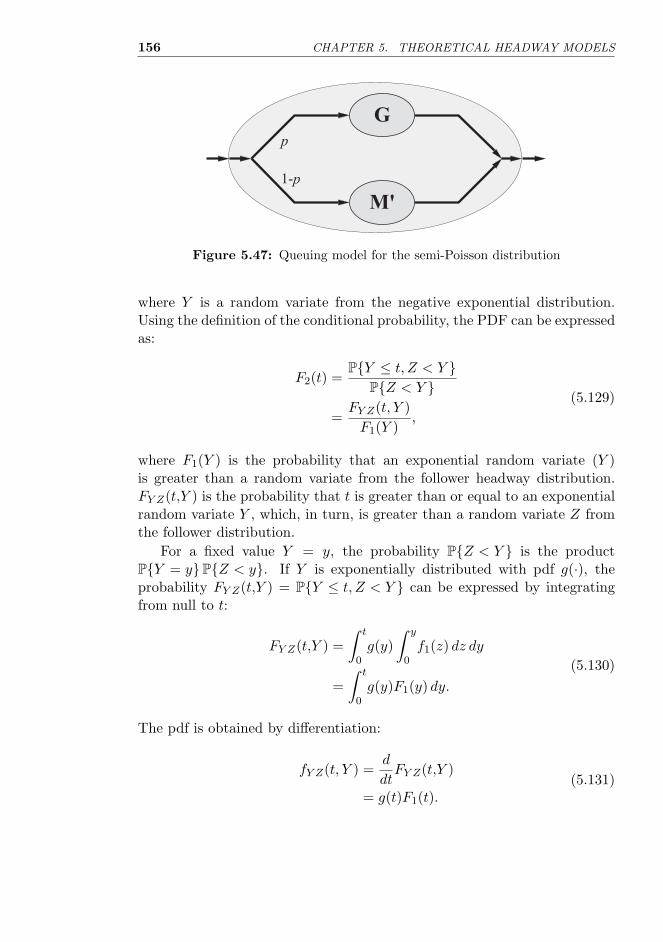
156 CHAPTER 5. THEORETICAL HEADWAY MODELS
1-p
p
G
M'
Figure 5.47: Queuing model for the semi-Poisson distribution
where Y is a random variate from the negative exponential distribution.Using the definition of the conditional probability, the PDF can be expressedas:
F2(t) =P{Y ≤ t, Z < Y }
P{Z < Y }=
FY Z(t, Y )F1(Y )
,
(5.129)
where F1(Y ) is the probability that an exponential random variate (Y )is greater than a random variate from the follower headway distribution.FY Z(t,Y ) is the probability that t is greater than or equal to an exponentialrandom variate Y , which, in turn, is greater than a random variate Z fromthe follower distribution.
For a fixed value Y = y, the probability P{Z < Y } is the productP{Y = y} P{Z < y}. If Y is exponentially distributed with pdf g(·), theprobability FY Z(t,Y ) = P{Y ≤ t, Z < Y } can be expressed by integratingfrom null to t:
FY Z(t,Y ) =∫ t
0g(y)
∫ y
0f1(z) dz dy
=∫ t
0g(y)F1(y) dy.
(5.130)
The pdf is obtained by differentiation:
fY Z(t, Y ) =d
dtFY Z(t,Y )
= g(t)F1(t).(5.131)

5.3. Mixed distributions 157
Consequently, the pdf for free headways is:
f2(t) =fY Z(t,Y )F1(Y )
=F1(t)F1(Y )
g(t).(5.132)
F1(Y ) is the probability that an exponential random variate (Y ) isgreater than a random variate (Z) from the follower distribution. Fora fixed value Y = y, the probability P{Y > Z} is equal to the productP{Y = y} P{Z < y}. If Y is exponentially distributed with scale parame-ter θ, the probability F1(Y ) can be expressed by integrating from null toinfinity:
F1(Y ) =∫ ∞
0θe−θy
∫ y
0f1(z) dz dy. (5.133)
Using the relation 29.2.6 of Abramowitz & Stegun (1972), this probabilityis the same as the Laplace transform of the follower distribution (Buckley1968):
F1(Y ) = f∗1 (θ). (5.134)
This leads to the equation for the free headway pdf:
f2(t) =F1(t)f∗1 (θ)
g(t). (5.135)
The Laplace transform can be derived using the same property 29.2.6 ofAbramowitz & Stegun (1972):
f∗2 (t) =
θ
f∗1 (θ)
∫ ∞
0e−(s+θ)t
∫ t
0f1(x) dx
=θ
s + θ· f∗
1 (s + θ)f∗1 (θ)
.
(5.136)
As Buckley (1968) has observed, the first term is the Laplace transformof the exponential distribution g(t) = θe−θt. Accordingly, the Laplace trans-form of the free headway distribution is the convolution of two distributions,namely g(t) and, say, c(t). Because c(t) has the Laplace transform:
c∗(s) =f∗1 (s + θ)f∗1 (θ)
, (5.137)

158 CHAPTER 5. THEORETICAL HEADWAY MODELS
it can be derived by the inverse transform (Buckley 1968):
c(t) =f1(t)f∗1 (θ)
e−θt. (5.138)
A free headway is thus a sum of two random variates, which follow thedistributions g(t) and c(t).
The pdf for the semi-Poisson distribution is (Buckley 1968):
f(t) = pf1(t) + (1 − p)F1(t)f∗1 (θ)
θe−θt, t ≥ 0, θ > 0, 0 ≤ p ≤ 1. (5.139)
The PDF is obtained by integration:
F (t) = pF1(t) +1 − p
f∗1 (θ)
∫ t
0F1(z)θe−θz dz, t ≥ 0, θ > 0, 0 ≤ p ≤ 1.
(5.140)The distribution has the Laplace transform (Buckley 1968):
f∗(s) = pf∗1 (t) + (1 − p)
θf∗1 (s + θ)
(s + θ)f∗1 (θ)
. (5.141)
Follower headway distribution
Buckley (1962) suggested the normal distribution as a model for followers’headways. He found that the error due to the non-zero probability of neg-ative headways was very small. Later Buckley (1968) applied gamma andtruncated normal distributions. He observed that gamma distribution hasthe general shape which is assumed to be correct for follower headways. Onthe other hand, he assumed that the truncated normal distribution coulddescribe the error in the tracking task, when a driver attempts to maintain adesired spacing. With gamma distributed follower headways Buckley couldnot obtain solutions for the parameters at low and low-medium flows. Whenthe parameters for both models were obtained, the model with gamma dis-tributed follower headways gave similar or better goodness of fit than thetruncated normal distribution.
Ashton (1971) saw no strong theoretical justification for choosing thenormal distribution. He chose gamma distribution because of its connectionwith the exponential distribution. Such a model should be theoreticallymore tractable. In the data analysis Ashton, however, used exponentialzone of emptiness.

5.3. Mixed distributions 159
Branston (1976) applied the model with the normal and the gamma dis-tributions for the follower headways. He estimated the parameters by com-bining the method of moments for p and θ with the minimum chi-squaremethod for β and α. He did not have similar difficulties as Buckley (1968).The goodness-of-fit was not acceptable, when the the normal distributionwas used for the follower headways. For gamma distributed follower head-ways he reported an acceptable goodness of fit.
Wasielewski (1974, 1979) calculated the distribution for the followerheadways directly from the empirical headway distribution without intro-ducing a parametric form. This nonparametric approach is not followed here,because in theoretical work and simulation a parametric model is preferable.
To sum up, normal, truncated normal, exponential, and gamma dis-tributions have been suggested as models for the follower headways. Theexponential distribution can describe the traffic flow with no vehicle inter-action, but it is unsuitable as a follower headway model. The studies ofBuckley and Branston suggest that the gamma distribution gives better re-sults than the normal and the truncated normal distributions. Lognormaldistribution would be theoretically an interesting alternative, but its useful-ness is limited, because it does not have a Laplace transform. Consequently,the gamma distribution was selected as the follower headway model.
The pdf (fig. 5.48) of the semi-Poisson distribution with gamma dis-tributed follower headways is:
f( t | p, β, α, θ ) = p(βt)α−1
Γ(α)βe−βt + (1 − p)
γ(α, βt)Γ(α)
(1 +
θ
β
)α
θe−θt,
t > 0; β, α, θ ≥ 0; 0 ≤ p ≤ 1, (5.142)
where γ(·) is the incomplete gamma function (see table 5.3, page 104). ThePDF is:
F( t | p, β, α, θ ) = pγ(α, βt)
Γ(α)+ (1 − p)
θ
Γ(α)
(1 +
θ
β
)α ∫ t
0γ(α, βu)e−θudu,
t > 0; β, α, θ ≥ 0; 0 ≤ p ≤ 1. (5.143)
Figure 5.49 shows the estimated semi-Poisson hazard function for sample 4.The Laplace transform of the semi-Poisson distribution is:
f∗(s) = p
(β
β + s
)α
+ (1 − p)θ
θ + s
(β + θ
β + θ + s
)α
. (5.144)
It is obvious that a free headway is a sum of two random variates: a variatefrom the exponential distribution and a variate from the gamma distribution

160 CHAPTER 5. THEORETICAL HEADWAY MODELS
0 2 4 6 8 100.0
0.1
0.2
0.3
0.4
Density
Follower headway component
Free headway component
Empirical headway density
Parameters:
p = 0.289
β = 5.488
α = 2.929
θ = 0.031
Semi-Poisson headway density
Figure 5.48: Semi-Poisson density function for sample 4
0 2 4 6 8 100.0
0.2
0.4
0.6
0.8
1.0
Hazard rate
Semi-Poisson hazard function
Empirical hazard function
Parameters:
p = 0.289
β = 5.488
α = 2.929
θ = 0.031
Figure 5.49: Semi-Poisson hazard function for sample 4
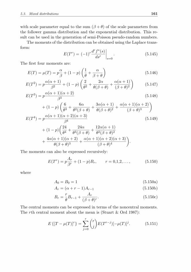
5.3. Mixed distributions 161
with scale parameter equal to the sum (β + θ) of the scale parameters fromthe follower gamma distribution and the exponential distribution. This re-sult can be used in the generation of semi-Poisson pseudo-random numbers.
The moments of the distribution can be obtained using the Laplace trans-form:
E(T r) = (−1)r drf∗(s)dsr
∣∣∣∣s=0
. (5.145)
The first four moments are:
E(T ) = µ(T ) = pα
β+ (1 − p)
(1θ
+α
β + θ
)(5.146)
E(T 2) = pα(α + 1)
β2 + (1 − p)(
2θ2 +
2α
θ(β + θ)+
α(α + 1)(β + θ)2
)(5.147)
E(T 3) = pα(α + 1)(α + 2)
β3 (5.148)
+ (1 − p)(
6θ3 +
6α
θ2(β + θ)+
3α(α + 1)θ(β + θ)2
+α(α + 1)(α + 2)
(β + θ)3
)
E(T 4) = pα(α + 1)(α + 2)(α + 3)
β4 (5.149)
+ (1 − p)(
24θ4 +
24α
θ3(β + θ)+
12α(α + 1)θ2(β + θ)2
+4α(α + 1)(α + 2)
θ(β + θ)3+
α(α + 1)(α + 2)(α + 3)(β + θ)4
).
The moments can also be expressed recursively:
E(T r) = pAr
βr+ (1 − p)Br, r = 0,1,2, . . . , (5.150)
where
A0 = B0 = 1 (5.150a)Ar = (α + r − 1)Ar−1 (5.150b)
Br =r
θBr−1 +
Ar
(β + θ)r. (5.150c)
The central moments can be expressed in terms of the noncentral moments.The rth central moment about the mean is (Stuart & Ord 1987):
E {[T − µ(T )]r} =r∑
j=0
(r
j
)E(T r−j)[−µ(T )]j . (5.151)

162 CHAPTER 5. THEORETICAL HEADWAY MODELS
Thus, the measures of dispersion can be calculated using the following equa-tions:
σ2(T ) = E{[T − µ(T )]2
}(5.152)
α3(T ) =E{[T − µ(T )]3
}σ3(T )
(5.153)
α4(T ) =E{[T − µ(T )]4
}σ4(T )
. (5.154)
Concerning the four-stage identification process, the following observa-tions can be made:
1. The pdf of the semi-Poisson distribution (figs. 5.48 and 5.50) is verysimilar to the empirical density function of the headway data.
2. The hazard rate (fig. 5.49) has the same properties as the empiricalhazard function. It starts from zero, rises to the maximum, falls, andreaches a constant level.
3. In terms of the coefficient of variation the semi-Poisson distribution isvery flexible.
4. Figure 5.51 shows the kurtosis of the semi-Poisson distribution againstthe squared skewness. The parameters were generated randomlywithin the limits displayed in the figure. The model can produce sam-ples such that the kurtosis corresponding to the squared skewness isonly slightly greater than the kurtosis of headway samples. When thedistribution approaches symmetry (α3 → 0), the kurtosis approachesthe values corresponding to the gamma distribution (see fig. 4.15 onpage 73). This is to be expected considering that α4 → 3 (see ta-ble 5.3 on page 104), and the distribution approaches normality as papproaches unity, and α tends to infinity (Johnson et al. 1994). Thefigure is very similar to the corresponding figure (5.46) of the general-ized queuing model.
The identification process indicates that the properties of the semi-Poissondistribution are very similar with the headway data. The KS2-chart displaysmost clearly the slight differences between the semi-Poisson distribution andthe headway data.

5.3. Mixed distributions 163
0 2 4 6 8 100.0
0.1
0.2
0.3
0.4
0.5
Headway [s]
Sample 32:
n = 390
λ = 795 veh/h
SL = 80 km/h
P(A-D) = 0.026
P(K-S) = 0.367
0 2 4 6 8 100.0
0.1
0.2
0.3
0.4
0.5
Headway [s]
0 2 4 6 8 100.0
0.1
0.2
0.3
0.4
0.5 Sample 62:
n = 150
λ = 143 veh/h
SL = 70 km/h
P(A-D) = 0.042
P(K-S) = 0.024
0 2 4 6 8 100.0
0.1
0.2
0.3
0.4
0.5 Sample 34:
n = 200
λ = 328 veh/h
SL = 50 km/h
P(A-D) = 0.475
P(K-S) = 0.709
Sample 25:
n = 900
λ = 1439 veh/h
SL = 80 km/h
P(A-D) = 0.002
P(K-S) = 0.181
Sample edf
Semi-
Poisson pdf
GOF estimate
Alternative estimate
Figure 5.50: Semi-Poisson pdf and sample edf. In sample 62 the “GOF esti-mate” shows the estimated pdf that was used in the goodness-of-fittests. The “alternative estimate” shows a better estimate, whichwas found using another starting point to find the maximum of theloglikelihood function.
0 5 10 15 20 25 30
0
10
20
30
40
50
Kurtosis
Parameters:
p ∈ (0,1)
β ∈ (0, 10)
α ∈ (1, 10)
θ ∈ (0, 0.56)Estimated headway kurtosis
Figure 5.51: KS2-chart of the semi-Poisson distribution with gamma distributedfollower headways (simulated data)

164 CHAPTER 5. THEORETICAL HEADWAY MODELS
Parameter estimation
Method of moments estimators According to Greenwood & Durand(1960) the method of moments is inefficient, except for distributions closelyresembling the normal. In this case the gamma distribution for followerheadways is expected to have a large shape parameter, which gives thedistribution the bell-like shape typical of the normal distribution. On theother hand, the method of moments gives good parameter estimates for thenegative exponential distribution also. Consequently, there are grounds forusing the method of moments to estimate the parameters of the gammadistribution.
The MME’s are obtained by equating the first four moments to thesample moments and solving simultaneously the parameter values. Buckley(1968) used this method to estimate the parameters. Because the simul-taneous equations were not explicitly solvable, he used numerical methods.He found no physically sensible solutions for flows less than 21 vehicles perminute (1,260 veh/h). The complicated form of the equations anticipatesevere difficulties in finding feasible parameter estimates.
Modified method of moments estimators To make the estimatorstractable, and to avoid the use of higher moments the method of momentscan be modified: Practically all headways in the exponential tail (ti > δ)belong to the free headway distribution. The PDF of the follower headwaysis then:
F1(t) = 1 − ε(t), when t > δ, (5.155)
where ε(t) is small. Now, p and θ can be estimated using the propertiesof the tail of the headway distribution, assuming that there are enoughobservations in the tail .
Let us assume a sample of size n with m observations greater than δ.The scale parameter estimate θ is the inverse of the modified sample meanof the tail (Wasielewski 1974, Wasielewski 1979):
θ =(
1m
n∑j=n−m+1
t(j) − δ
)−1
, (5.156)
where t(j) is the jth order statistic of the sample.

5.3. Mixed distributions 165
The probability that a headway belongs to the tail of the distribution is:
P{T > δ} =∫ ∞
δf(t) dt
= p
∫ ∞
δf1(t) dt +
(1 − p)f∗1 (θ)
∫ ∞
δF1(t)θe−θtdt
= p[1 − F1(δ)] +(1 − p)f∗1 (θ)
∫ ∞
δF1(t)θe−θtdt.
(5.157)
If t > δ , the follower headway PDF is near unity (F1(t) ≈ 1), and theequation simplifies to
P{T > δ} =1 − p
f∗1 (θ)
e−θδ
= (1 − p)(
1 +θ
β
)α
e−θδ
(5.158)
The proportion of headways in the tail can be used as an estimate forthe probability P{T > δ}. This leads to the following estimator for p:
p = 1 − m
n
(1 +
θ
β
)−α
eθδ. (5.159)
The system of equations can be completed by equating the first two momentsto the corresponding sample moments:
m′1 = t = p
α
β+ (1 − p)
(1θ
+α
β + θ
)(5.160)
m′2 = p
α(α + 1)β2
+ (1 − p)(
2θ2
+2α
θ + (β + θ)+
α(α + 1)(β + θ)2
). (5.161)
Branston (1976) estimated θ and p from these two equations. He thenestimated β and α by minimizing the chi-square statistic.
The equation for the first moment can be solved to obtain the estimatorfor the shape parameter:
α =β(β + θ)[m′
1θ − (1 − p)]θ(β + pθ)
. (5.162)
The he scale parameter estimator is the solution to the polynomial equa-tion, which is obtained by substituting for α in the equation for the second

166 CHAPTER 5. THEORETICAL HEADWAY MODELS
moment:
[(m′21 − m2)θ2 + 1 − p2]β4
+ {(1 − 2p)(m′21 − m2)θ2 + [1 − 2p(1 − p)]m′
1θ + 5p(1 − p)}θβ3
+ {[3m′21 − (2 + p)m′
2]θ2 + (4p − 1)m′
1θ + 2 − p(1 − p)}pθ2β2
+ [(m′21 − m′
2p)θ2 + (4p − 1)m′1θ − p(1 − p)]pθ3β
+ [m′1θ − (1 − p)]p2θ4 = 0. (5.163)
This equation has two unknown parameter estimates (p and β). Becausethis is a fourth degree polynomial, its roots can be solved, assuming eitherp or β known. There is an analytic solution to the equation with hundredsof terms (obtained by the Maple computer algebra system), but it was notused, because there are well tested, fast and accurate numerical methods forfinding the roots of a polynomial.
Assuming p known, α and β can be solved using equations (5.162) and(5.163). The estimate is accepted, if the absolute error in the estimate of pis smaller than the criterion of precision:∣∣∣∣∣∣1 − m
n
(1 +
θ
β
)−α
eθδ − p
∣∣∣∣∣∣ < ε. (5.164)
The problem with this method is that β is not a real number for allvalues of p. Unfortunately, this often occurs with such values of p that wouldresult in smallest estimation errors. Consequently, the modified method ofmoments was rejected.
Maximum likelihood estimators The likelihood function of the semi-Poisson distribution with gamma distributed follower headways is:
L(p, β, α, θ) =n∏
j=1
f( tj | p, β, α, θ )
=(
1Γ(α)
)n n∏j=1
[p(βtj)α−1βe−βtj
+ (1 − p)γ(α, βtj)(
1 +θ
β
)α
θe−θtj
]. (5.165)

5.3. Mixed distributions 167
The log-likelihood function is:
lnL(p, β, α, θ) = −n ln Γ(α) +n∑
j=1
ln[p(βtj)α−1βe−βtj
+ (1 − p)γ(α, βtj)(
1 +θ
β
)α
θe−θtj
]. (5.166)
The maximum likelihood estimators are obtained by equating to zerothe gradient of the log-likelihood function and solving the resulting set ofequations. This must be done by numerical methods.
A modified method was also tested, in which the exponential scale pa-rameter was estimated from the tail using equation (5.156). This methoddecreased the dimensionality of the problem, but there was no significantincrease in speed and the results were less accurate. Accordingly, the maxi-mum likelihood method was used without any modifications.
In some cases, the results were sensitive to the starting point (seefig. 5.50).14 Because the calculations were very time consuming, only onestarting point was tried. The parameter estimation of sample 59 failed. Infive samples (26, 38, 45, 46, and 62) p was either unity or null.
Figures 5.52 and 5.53 show the parameter estimates for the headwaydata, excluding the six samples listed above. On low speed roads there issignificant correlation between p and volume (r = 0.734, P < 0.0005), andbetween θ and volume (r = 0.920, P < 0.0005). That is, the proportion offollower headways increases with increasing traffic volume. Also, the propor-tion of short free headways increases. On high speed roads the correlationbetween θ and the volume is also strong (r = 0.810, P < 0.0005). For p thecorrelation is not as strong, but it is still statistically significant (r = 0.511,P = 0.004).
The parameters of the gamma distribution do not correlate with trafficvolume, but they have a strong mutual correlation (figure 5.54). The ratioβ/α is relatively constant, being 0.60 on low speed roads and 0.59 on highspeed roads. The difference is not statistically significant (P = 0.62), butthe follower flow rate is about 2,140 veh/h on both low speed and high speedroads. The estimate does not change with the overall traffic flow rate. Thefollower flow rate is near the capacity estimate of 2,200 person cars per hourper lane on multilane highways (HCM 1994).
14Branston (1976) also encountered instability in the parameter estimates.

168 CHAPTER 5. THEORETICAL HEADWAY MODELS
0 500 1 000 1 500
0.0
0.1
0.2
0.3
0.4
0.5
0.6
Volume [veh/h]
θ
50-70 km/h 80-100 km/h
0 500 1 000 1 500
0.0
0.2
0.4
0.6
0.8
1.0
Volume [veh/h]
p
50-70 km/h 80-100 km/h
^^
Figure 5.52: Maximum likelihood estimates for p and θ
0 500 1 000 1 500
0
2
4
6
8
10
12
14
Volume [veh/h]
α
50-70 km/h 80-100 km/h
0 500 1 000 1 500
0
2
4
6
8
10
12
14
Volume [veh/h]
β
50-70 km/h 80-100 km/h
^^
Figure 5.53: Maximum likelihood estimates for β and α

5.3. Mixed distributions 169
0 2 4 6 8 10 12 14
0
2
4
6
8
10
12
β
Speed limit
50-70 km/h
80-100 km/h
^
^
Figure 5.54: α against β
Goodness-of-fit tests
The parameters were estimated using the maximum likelihood method.Sample 59 was excluded, because its parameter estimation failed. The good-ness of fit was tested using both the nonparametric K-S test and the para-metric A-D test. The parametric test was conducted using the Monte Carlomethod described in section 2.2.4.
For each of the 62 samples, 500 replications were generated and analyzed.The number of replications was low, because the parameter estimation wasvery time consuming.15 If the parameter estimation of a replication failed, anew replication was generated. If more than 25 (5 %) failures were recorded,the goodness-of-fit test was discarded. Four samples (38, 56, 61, and 64)failed the test procedure.
Figure 5.55 shows the goodness-of-fit test results for the semi-Poissondistribution with gamma distributed zone of emptiness. There is an inter-esting difference in the figures: The significance probabilities of the K-Stests are mostly between 0.2 and 0.8, while the A-D tests produce signif-icance probabilities which are mostly either below 0.3 or above 0.6. Thecomparison of the results (fig. 5.56) shows that the 5 % significance levelof the parametric A-D test is about the same as the 40 % significance levelof the nonparametric K-S test. Consequently, the semi-Poisson distribution
15It took three weeks to perform the goodness-of-fit tests on three i386/i486 personalcomputers.

170 CHAPTER 5. THEORETICAL HEADWAY MODELS
0 500 1 000 1 500
0.0
0.2
0.4
0.6
0.8
1.0
Volume [veh/h]
P(K-S)
50-70 km/h 80-100 km/h
0 500 1 000 1 500
0.0
0.2
0.4
0.6
0.8
1.0
Volume [veh/h]
P(A-D)
50-70 km/h 80-100 km/h
Figure 5.55: Goodness-of-fit tests for the semi-Poisson distribution
fits the data extremely well, but it appears to be caused more by the flexi-bility of the model than by its inherently correct shape. As the flexibility ofthe model increases, the bias in the nonparametric EDF tests also increases.
The combined probability of the nonparametric K-S tests is 0.85. Theparametric A-D tests, however, give combined probability of only 4.3 ·10−11.The fit is best, when the data have large sample variance. When the varianceis larger than 100, the significance probability of the sample is greater than0.1. Only sample 62 is an exception, but it is probably caused by theunsuccessful parameter estimation. On the other hand, all the eight samplesof at least 500 observations have significance probability less than 0.1. Thesesamples are from high speed roads. Accordingly, the semi-Poisson model fitsbest small samples with large variances.16 In such cases the “noise” in thedata hides small bias in the model.
Semi-Poisson distribution in headway studies
Reasonability The modification of the free headway distribution f2(t) inthe semi-Poisson model can be criticized: The condition that a free head-
16The data do not contain large (> 500) samples with large variances (> 100).

5.3. Mixed distributions 171
0.0 0.2 0.4 0.6 0.8 1.0
0.0
0.2
0.4
0.6
0.8
1.0
P(A-D)
Figure 5.56: Comparison of the nonparametric K-S and the parametric A-D testsfor the semi-Poisson distribution
way should be greater than a random variate from the constrained head-way distribution f1(t) seems arbitrary, because the shape of the constrainedheadway distribution is not necessarily the way that the frequency of freeheadways decreases near the origin. The process of becoming a follower isnot equal to adjusting the headway while being a follower.
Branston (1976) describes the difference between the semi-Poisson modeland the M/G/1 queuing model as follows:
In the semi-Poisson model each free headway is obtained by com-paring an exponential headway with a following headway, whilein the queuing model each free headway is obtained by addingan exponential gap to a following headway.
This description overstates the difference between these distributions. Thenonfollower headway variate in the semi-Poisson distribution is also a sumof an exponential random variate and another random variate (see equation5.138). In fact, the M/G/1 model and the semi-Poisson distribution donot differ significantly when realistic parameter values are used (Botma &Fi 1991).
Applicability Parameter estimation is time consuming, but semi-Poissonpseudorandom numbers can be generated efficiently (Buckley 1962). Thepdf is rather complicated, and the PDF must be solved numerically. Nowthat numerical integration is widely available in personal computers and

172 CHAPTER 5. THEORETICAL HEADWAY MODELS
even in pocket calculators, there are better potentials for the application ofthe semi-Poisson distribution. The Laplace transform exists, if it exists forthe follower headway distribution.
Validity The chi-square tests of Buckley (1968) gave all “good” results.Branston (1976) reported an average probability of 0.196 for 16 chi-squaretests (M4 fast lane). The combined probability, however, is only 0.0004. Fornormal zone of emptiness the results were even worse.
The semi-Poisson distribution yields a better fit than any of the simpledistributions. If the K-S tests give as good results as shown above, but thehypothesis is still rejected, the distribution is likely to be so flexible that anextremely good fit is required. So good a fit may be impossible for headwaydata, where some disturbances cannot always be avoided.
Chapter 6
Conclusions andrecommendations
The main purpose of the study was to present methods in order to improvethe statistical analysis of vehicle headways. A more firm scientific foundationhas been laid for further studies. Also, some new information about theproperties of vehicle headways on two-lane two-way roads has been obtained.
The combined probabilities method of Fisher (1938) provided a scientif-ically sound method to test a hypothesis on a multi-sample data set. Themethod was used extensively throughout the research. It was also demon-strated that in many earlier headway studies this method would have beenof great help—either further confirming the results or guarding from falseconclusions. The combined probabilities method should be routinely usedin the tests for multi-sample data.
The combined probabilities method forms the basis of the moving proba-bility method (Luttinen 1992), which appeared to be very helpful in demon-strating the variation of test results over traffic volumes. This new methodprovided results not directly available with the traditional methods. It canbe assumed that the method will have much wider applications in statis-tics. However, the experience with the method is still limited, and furtherresearch is needed.
The first step in the empirical research (fig. 1.1, page 20) is the datacollection. A major problem in the collection of headway data is to obtainstationary data. It was shown that the combination of small samples withnearly equal means produces a biased data set. This bias can be avoided,if the data collection is based on trend analysis. Tests against trend shouldbecome a standard procedure in headway studies.
173

174 CHAPTER 6. CONCLUSIONS AND RECOMMENDATIONS
In model identification it is important to find a few methods that showthe most important properties of the data. For the identification of headwaymodels a four-stage identification process was proposed. It includes theestimation of:
1. Probability density function
2. Hazard function
3. Coefficient of variation (CV-chart)
4. Kurtosis and squared skewness (KS2-chart).
The probability density function displays the shape of the distributionbetter than the probability distribution function. The hazard function ismostly used in life and reliability data analysis, but it also very informativein headway studies. The kernel method was shown to produce smooth es-timates for density and hazard functions. It should be preferred over themore traditional histogram method.
The coefficient of variation is a scaled measure of the variation in head-ways. It is a useful measure of dispersion in the headway distribution. Thecorrelation between the kurtosis and the squared skewness was very highin the headway data. A KS2-chart displays clearly differences between theheadway data and statistical models.
The four-stage identification process allows an effective statistical de-scription of the headway data. The process also shows many advantages anddisadvantages of the theoretical statistical distributions when compared tothe headway data. Moreover, the comparison of data from different sourceswould be easier, if the data were submitted to standard analyses. The four-stage identification process is suggested as a framework for future studies.
The independence of consecutive headways was tested using the auto-correlation analysis, runs tests, and goodness-of-fit tests for the geometricplatoon length distribution. The power of the tests was enhanced by com-bining the significance probabilities of each sample into a single significancemeasure. The variation of significance over traffic volumes was describedand the evidence made stronger by the moving probability methods. Theresults indicate that the renewal hypothesis should not be accepted in alltraffic situations, although the possible autocorrelation is weak.
Concerning the parameter estimation, two properties of the headwaydistributions are worth consideration:
1. The headway distributions are strongly skewed to the right.

175
2. The headways of trailing vehicles have a practical minimum.
Because of the skewness of the headway distribution, the method of mo-ments does not give as good estimates as the maximum likelihood method.Because of the practical minimum headway, a location parameter (τ) is oftenincluded in the headway models. In some cases no solutions can be foundfor the maximum likelihood equations of such models. The modified maxi-mum likelihood method was shown to produce good parameter estimates fordistributions with a location parameter.
The main problems of the goodness-of-fit tests in headway studies are:
1. The chi-square test is based on grouping of the data. This makes thetest less powerful than the tests based on the empirical distributionfunction (EDF).
2. The nonparametric goodness-of-fit tests based on the EDF can beapplied only, when the parameters of the distribution are known. Ifthe parameters of the headway distributions must be estimated fromthe data, the nonparametric tests give too conservative results.
3. When the parameters are estimated from the data, parametric EDFtests should be used. The distribution of the test statistic is, however,not known.
These problems were conquered using parametric EDF test and estimat-ing the distribution of the test statistic by Monte Carlo methods. The supe-riority of these tests over the nonparametric Kolmogorov-Smirnov tests wasdemonstrated. The power of the tests was further enhanced by combiningthe significance probabilities of all samples. It is suggested that the goodnessof fit should be measured by both the nonparametric Kolmogorov-Smirnovtest and by some parametric EDF test. The parametric Anderson-Darlingtest is recommended. The conclusions should be based on the parametrictest, but the nonparametric test gives an overall goodness-of-fit measureagainst which different models can be compared. This helps to find out ifthe problem in the model is lack of fit, or flexibility of the model, whichpresents higher requirements for the fit.
Three principles of evaluation were suggested to evaluate the headwaydistribution models:
1. Reasonability. It is an advantage if the structure of the modelis based on explicit theoretical reasoning about the characteristics oftraffic flow.

176 CHAPTER 6. CONCLUSIONS AND RECOMMENDATIONS
2. Applicability. The model should have a simple structure to avoidinsurpassable problems in mathematical analysis. If simulation is con-sidered, the generation of pseudo-random variates should be fast andreliable. Parameter estimation should not be too complicated.
3. Validity. The model should give a good approximation of the realworld phenomena. This can be tested first by the four-stage identifi-cation process and finally by the goodness-of-fit tests.
Five statistical distributions were evaluated as models for the headwaydistributions on two-lane roads. The results of the goodness-of-fit tests1 arepresented in table 6.1.
Table 6.1: Summary of the goodness-of-fit tests
Distribution P(K-S) P(A-D)Negative exponential 2.1 · 10−162 2.9 · 10−150
Shifted exponential 3.8 · 10−157 5.3 · 10−150
Gamma 8.7 · 10−106 4.1 · 10−141
Lognormal 1.8 · 10−36 1.8 · 10−114
Semi-Poisson 0.85 4.3 · 10−11
The exponential distribution can be considered as a model for vehicleheadways under extremely low flow conditions, and for applications thatare not very sensitive to the shape of the headway distribution. In somecases the analytical solution of the problem may only be possible with avery simple model. In such situations the limitations of the model shouldbe clearly indicated.
The shifted exponential distribution does not produce extremely shortheadways, which is a major problem in the negative exponential distribu-tion. The goodness of fit is, however, not significantly better. The shiftedexponential distribution can be used in similar situations as the negativeexponential distribution, especially when it is important to set a minimumheadway.
The gamma distribution can be used, if the distribution should have asimple form and low probability for short headways, and the results are nottoo sensitive to other properties of the distribution. Under low-to-moderate
1The precision of the Kolmogorov-Smirnov tests was four decimals. If a test result was0.0000, the combined probability was calculated using 0.000025 in stead.

177
traffic volumes the use of the gamma distribution can be given preferenceover the exponential distribution.
The lognormal distribution falls between the simple-nonrealistic andcomplex-realistic models. The goodness-of-fit results are better than forthe other simple distributions, but mathematical analysis presents someproblems. There are, however, some theoretical reasons to consider thelognormal distribution as a model for the follower headway distribution(Daou 1966, Greenberg 1966).
The semi-Poisson distribution can be recommended for demanding ap-plications with adequate computational facilities. It produced the best testresults, but even it failed the parametric test.
The data in this study are from Finnish two-lane two-way roads. Suchfactors as speed limit, passing sight distance, lane and shoulder width, climb-ing lanes, proportion of heavy vehicles, flow rate of opposite traffic, trafficsignals, distance to major traffic generators, and intersection density havean effect on the headway distribution. Our knowledge of these relationshipsis, however, very limited. The headway distribution model should be veryadaptive, but not too flexible. It should have all the right parameters, butnone too many. In this respect all the work toward a unified traffic flowtheory is most welcome.
The proposed procedures give a scientific foundation to identify andestimate statistical models for vehicle headways, and to test the goodness offit. It has been shown that the statistical methods in the analysis of vehicleheadways should be thoroughly revised following the guidelines presented inthis text.


References
Abramowitz, M. & Stegun, I. A. (1972), Handbook of Mathematical Func-tions with Formulas, Graphs, and Mathematical Tables, Dover Publi-cations, Inc., New York. 9th printing.
Adams, W. F. (1936), ‘Road traffic considered as a random series’, Journalof the Institution of Civil Engineers 4(1), 121–130.
Akcelik, R. & Chung, E. (1994), ‘Calibration of the bunched exponentialdistribution of arrival headways’, Road & Transport Research 3(1), 42–59.
Anderson, T. & Darling, D. (1952), ‘Asymptotic theory of certain “goodnessof fit” criteria based on stochastic processes’, The Annals of Mathemat-ical Statistics 23, 193–212.
Ashton, W. D. (1971), ‘Distribution for gaps in road traffic’, J. Inst. MathsApplics 7, 37–46.
Baerwald, J. E., ed. (1976), Transportation and Traffic Engineering Hand-book, Prentice-Hall, Inc., Englewood Cliffs, N.J.
Bai, J., Jakeman, A. J. & Taylor, J. A. (1990), ‘Percentile estimation ofthe three-parameter gamma and lognormal distributions: Methods ofmoments versus maximum likelihood’, Mathematics and Computers inSimulation 32(1&2), 167–172.
Baras, J. S., Dorsey, A. J. & Levine, W. S. (1979a), ‘Estimation of traf-fic platoon structure from headway statistics’, IEEE Transactions onAutomatic Control 24(4), 553–559.
Baras, J. S., Levine, W. S. & Lin, T. L. (1979b), ‘Discrete-time point pro-cesses in urban traffic queue estimation’, IEEE Transactions on Auto-matic Control. 24(1), 12–27.
179

180 REFERENCES
Betro, B., Schoen, F. & Speranza, M. G. (1987), A stochastic environ-ment for the adaptive control of single intersections, in N. H. Gartner& N. H. M. Wilson, eds, ‘Transportation and Traffic Theory’, Pro-ceedings of the Tenth International Symposium on Transportation andTraffic Theory, held July 8–10, 1987, at the Massachusetts Institute ofTechnology, Cambridge, Massachusetts, Elsevier, New York.
Botma, H. (1986), Traffic operations on busy two-lane rural roads in theNetherlands, in ‘Traffic Flow Theory, Characteristics, and HighwayCapacity’, number 1091 in ‘Transportation Research Record’, Trans-portation Research Board, Washington, D.C., pp. 126–131.
Botma, H. & Fi, I. (1991), Traffic operation on 2-lane roads in Hungary andthe Netherlands, in Brannolte (1991), pp. 41–53.
Bowman, K. O. & Shenton, L. R. (1988), Properties of Estimators for theGamma Distribution, Marcel Dekker, Inc., New York.
Brannolte, U., ed. (1991), Highway Capacity and Level of Service, Balkema,Rotterdam.
Branston, D. (1976), ‘Models of single lane time headway distributions’,Transportation Science 10(2), 125–148.
Branston, D. (1979), ‘A method of estimating the free speed distribution fora road’, Transportation Science 13(2), 130–145.
Breiman, L. (1963), ‘The Poisson tendency in traffic distribution’, The An-nals of Mathematical Statistics 32, 308–311.
Breiman, L., Gafarian, A. V., Lichtenstein, R. & Murthy, V. K. (1969),An experimental analysis of single-lane time headways in freely flowingtraffic, in Leutzbach & Baron (1969), pp. 22–29.
Breiman, L., Lawrence, R., Goodwin, D. & Bailey, B. (1977), ‘The statisticalproperties of freeway traffic’, Transportation Research 11A(4), 221–228.
Brockwell, P. J. & Davis, R. A. (1987), Time Series: Theory and Methods,Springer Verlag, New York.
Buckley, D. J. (1962), Road traffic headway distributions, in ‘Proceedings’,Vol. 1, part 1, Australian Road Research Board, Victoria, pp. 153–187.

181
Buckley, D. J. (1968), ‘A semi-Poisson model of traffic flow’, TransportationScience 2(2), 107–133.
Bureau of Public Roads (1950), Highway Capacity Manual, U.S. Departmentof Commerce, Washington, D.C.
Chandler, R. E., Herman, R. & Montroll, E. W. (1958), ‘Traffic dynamics:Studies in car following’, Operations Research 6(2), 165–184.
Chishaki, T. & Tamura, Y. (1984), Headway distribution model based on thedistinction between leaders and followers, in J. Volmuller & R. Hamer-slag, eds, ‘Proceedings of the Ninth International Symposium on Trans-portation and Traffic Theory’, VNU Science Press, Utrecht, pp. 43–63.
Chrissikopoulos, V., Darzentas, J. & McDowell, M. (1982), ‘Aspects of head-way distributions and platooning on major roads’, Traffic Engineeringand Control 23(5), 268–271.
Cochran, J. K. & Cheng, C.-S. (1989), ‘Automating the procedure for an-alyzing univariate statistics in computer simulations contexts’, Trans-actions of the Society for Computer Simulation 6(3), 173–188.
Cohen, A. C. & Whitten, B. J. (1980), ‘Estimation in the three-parameterlognormal distribution’, Journal of the American Statistical Association75(370), 399–404.
Cohen, A. C. & Whitten, B. J. (1982), ‘Modified moment and maximumlikelihood estimators for parameters of the three-parameter gamma dis-tribution’, Communications in Statistics: Simulation and Computation11(2), 197–216.
Cohen, A. C. & Whitten, B. J. (1988), Parameter Estimation in Reliabilityand Life Span Models, Marcel Dekker, Inc., New York.
Conover, W. (1980), Practical Nonparametric Statistics, second edn, JohnWiley & Sons, New York.
Cooper, R. B. (1981), Introduction to Queueing Theory, second edn, EdwardArnold (Publishers) Limited, London.
Cowan, R. (1978), ‘An improved model for signalized intersections withvehicle-actuated control’, Journal of Applied Probability 15, 384–396.
Cowan, R. J. (1975), ‘Useful headway models’, Transportation Research9(6), 371–375.

182 REFERENCES
Cox, D. R. & Hinkley, D. (1974), Theoretical Statistics, Chapman and Hall,London.
Cox, D. R. & Lewis, P. A. W. (1966), The Statistical Analysis of Series ofEvents, Methuen & Co Ltd., London.
Cox, D. R. & Stuart, A. (1955), ‘Some quick sign tests for trend in locationand dispersion’, Biometrika 42, 80–95.
Crow, E. L. & Shimizu, K., eds (1988), Lognormal Distributions: Theoryand Applications, Marcel Dekker, Inc., New York.
D’Agostino, R. B. & Stephens, M. A., eds (1986), Goodness-of-Fit Tech-niques, Marcel Dekker, Inc., New York.
Daley, D. & Vere-Jones, D., eds (1988), An Introduction to the Theory ofPoint Processes, Springer Verlag, New York.
Daou, A. (1964), ‘The distribution of headways in a platoon’, OperationsResearch 12(2), 360–361.
Daou, A. (1966), ‘On flow within platoons’, Australian Road Research2(7), 4–13.
Darroch, J. N., Newell, G. F. & Morris, R. W. J. (1964), ‘Queues for avehicle-actuated traffic light’, Operations Research 12(6), 882–895.
Dawson, R. F. (1969), The hyperlang probability distribution - a generalizedtraffic headway model, in Leutzbach & Baron (1969), pp. 30–36.
Dawson, R. F. & Chimini, L. A. (1968), The hyperlang probabilitydistribution—A generalized traffic headway model, in ‘Characteristicsof Traffic Flow’, number 230 in ‘Highway Research Record’, HighwayResearch Board, Washington, D.C., pp. 1–14.
Drew, D. R. (1967), Gap acceptance characteristics for ramp-freeway surveil-lance and control, in ‘Freeway Traffic Characteristics and Control’,number 157 in ‘Highway Research Record’, Highway Research Board,Washington, D.C., pp. 108–143. With discussion.
Drew, D. R. (1968), Traffic Flow Theory and Control, McGraw-Hill, NewYork.
Dudewicz, E. J. & Mishra, S. N. (1988), Modern Mathematical Statistics,John Wiley & Sons, New York.

183
Dunne, M. C., Rothery, R. W. & Potts, R. B. (1968), ‘A discrete Markovmodel of vehicular traffic’, Transportation Science 2(3), 233–251.
Durbin, J. (1975), ‘Kolmogorov-Smirnov tests when parameters are esti-mated with applications to tests of exponentiality and tests on spac-ings’, Biometrika 62(1), 5–22.
Enberg, A. & Pursula, M. (1991), Traffic flow and level of service on high-class two-lane rural roads in Finland, in Brannolte (1991), pp. 119–126.
Enberg, A. & Pursula, M. (1992), Moottoriliikennetien liikennevirran omi-naisuudet [Basic characteristics of traffic flow on high-class two-lanerural roads in Finland], number 12/1992 in ‘Tielaitoksen selvityksia’,Tielaitos, Helsinki.
Fisher, R. A. (1938), Statistical Methods for Research Workers, seventh edn,Oliver and Boyd, Edinburgh.
Galin, D. (1980), ‘A comparison of some bunch-size models for two-lane ruralroads - an Israeli experience’, Transportation Research 14A(1), 51–56.
Garwood, F. (1940), ‘An application of the theory of probability to theoperation of vehicular-controlled traffic signals’, Journal of the RoyalStatistical Society 7(1), 65–77.
Gazis, D. G., Herman, R. & Potts, Renfrey, B. (1959), ‘Car-following theoryof steady-state traffic flow’, Operations Research 7(4), 499–505.
Gazis, D. G., Herman, R. & Rothery, R. W. (1961), ‘Nonlinear follow-the-leader models of traffic flow’, Operations Research 9(4), 545–567.
Gill, P. E., Murray, W. & Wright, M. H. (1981), Practical Optimization,Academic Press, London.
Gradshteyn, I. S. & Ryzhik, I. M. (1980), Table of Integrals, Series, andProducts, Academic Press, New York. Corrected and enlarged editionprepared by Alan Jeffrey.
Grecco, W. L. & Sword, E. C. (1968), ‘Prediction of parameters for Schuhl’sheadway distribution’, Traffic Engineering 38, 36–38.
Green, J. R. & Hegazy, Y. A. S. (1976), ‘Powerful modified-EDFgoodness-of-fit tests’, Journal of the American Statistical Association71(353), 204–209.
184 REFERENCES
Greenberg, I. (1966), ‘The log-normal distribution of headways’, AustralianRoad Research 2(7), 14–18.
Greenwood, J. A. & Durand, D. (1960), ‘Aids for fitting the gamma distri-bution by maximum likelihood’, Technometrics 2(1), 55–65.
Griffiths, J. D. & Hunt, J. G. (1991), ‘Vehicle headways in urban areas’,Traffic Engineering and Control 32(10), 458–462.
Gross, D. & Harris, C. M. (1985), Fundamentals of Queueing Theory, secondedn, John Wiley & Sons, New York.
HCM (1965), Highway Capacity Manual, number 87 in ‘Special Report’,Highway Research Board,National Research Council, Washington, D.C.
HCM (1985), Highway Capacity Manual, number 209 in ‘Special Report’,Transportation Research Board, National Research Council, Washing-ton, D.C.
HCM (1994), Highway Capacity Manual, number 209 in ‘Special Report’,third edn, Transportation Research Board, National Research Council,Washington, D.C. Updated October 1994.
Heidemann, D. (1990), A theoretical model to calculate time-headway distri-butions as a function of traffic density, in M. Koshi, ed., ‘Transportationand Traffic Theory’, Proceedings of the Eleventh International Sympo-sium on Transportation and Traffic Theory, held July 18–20, 1990, inYokohama, Japan, Elsevier, New York, pp. 1–17.
Heidemann, D. (1993), A theoretical model for distributions of speeds andtime-headways on two-lane roads, in C. F. Daganzo, ed., ‘Transporta-tion and Traffic Theory’, Proceedings of the 12th International Sympo-sium on Transportation and Traffic Theory, Berkeley, California, USA,21–23 July, 1993, Elsevier, Amsterdam, pp. 523–537.
Herman, R. & Potts, R. B. (1961), Single-lane traffic theory and experiment,in R. Herman, ed., ‘Theory of Traffic Flow’, Proceedings of the Sympo-sium on the Theory of Traffic Flow, Elsevier, Amsterdam, pp. 120–146.
IMSL (1989), IMSL STAT/LIBRARY. Version 1.1, IMSL, Inc., Houston,Texas.
Johnson, N. L., Kotz, S. & Balakrishnan, N. (1994), Continuous UnivariateDistributions, Vol. 1, second edn, John Wiley & Sons, New York.

185
Kalbfleisch, J. D. & Prentice, R. L. (1980), The Statistical Analysis of FailureTime Data, John Wiley & Sons, New York.
Kell, J. H. (1962), Analyzing vehicular delay at intersections through sim-ulation, in ‘Theory of Traffic Flow’, number 356 in ‘Highway ResearchBoard Bulletin’, Highway Research Board, Washington, D.C., pp. 28–39.
Kendall, M. & Ord, J. K. (1990), Time-Series, third edn, Edward Arnold,London.
Khintchine, A. Y. (1960), Mathematical Methods in the Theory of Queueing,Charles Griffin Ltd., London. Translated by D. M. Andrews and M. H.Quenouille.
Kikuchi, S. & Chakroborty, P. (1992), Car-following model based on fuzzyinference system, in ‘Highway Capacity and Traffic Flow’, number 1365in ‘Transportation Research Record’, Transportation Research Board,Washington, D.C., pp. 82–91.
Kingman, J. F. C. (1962), ‘On queues in heavy traffic’, Journal of the RoyalStatistical Society 24(2), 383–392.
Kleinrock, L. (1975), Queueing Systems. Volume I: Theory, John Wiley &Sons, New York.
Leutzbach, W. (1988), Introduction to the Theory of Traffic Flow, SpringerVerlag, Berlin.
Leutzbach, W. & Baron, P., eds (1969), Beitrage zur Theorie des Verkehrs-flusses, number 86 in ‘Strassenbau und Strassenverkehrstechnik’, Bun-desminister fur Verkehr, Bundesminister fur Verkehr, Bonn.
Lilliefors, H. W. (1967), ‘On the Kolmogorov-Smirnov test for normalitywith mean and variance unknown’, American Statistical AssociationJournal 62, 399–402.
Lilliefors, H. W. (1969), ‘On the Kolmogorov-Smirnov test for the exponen-tial distribution with mean unknown’, American Statistical AssociationJournal 64, 387–389.
Lin, F. (1985a), ‘Relationships between queueing flows and presence detec-tors’, ITE Journal pp. 42–46.

186 REFERENCES
Lin, F.-B. (1985b), Evaluation of queue dissipation simulation models foranalysis of presence-mode full-actuated signal control, in ‘HighwayCapacity, Traffic Characteristics, and Flow Theory’, number 1005in ‘Transportation Research Record’, Transportation Research Board,Washington, D.C., pp. 46–54.
Luttinen, R. T. (1990), Johdatus aikavalijakaumien teoriaan [Introductionto the theory of headway distributions], Julkaisu 71, Teknillinen kor-keakoulu, Liikennetekniikka, Otaniemi.
Luttinen, R. T. (1991), Testing goodness of fit for 3-parameter gamma dis-tribution, in ‘Proceedings of the Fourth IMSL User Group Europe Con-ference’, IMSL and CRPE-CNET/CNRS, Paris, pp. B10/1–13.
Luttinen, R. T. (1992), Statistical properties of vehicle time headways, in‘Highway Capacity and Traffic Flow’, number 1365 in ‘TransportationResearch Record’, Transportation Research Board, Washington, D.C.,pp. 92–98.
Luttinen, R. T. (1994), Identification and estimation of headway distribu-tions, in R. Akcelik, ed., ‘Second International Symposium on HighwayCapacity’, Australian Road Research Board, Transportation ResearchBoard, Sydney, pp. 427–446.
Madansky, A. (1988), Prescriptions for Working Statisticians, Springer Ver-lag, New York.
May, A. (1961), ‘Traffic characteristics and phenomena on high density con-trolled access facilities’, Traffic Engineering 31(6), 11–19.
May, A. D. (1965), Gap availability studies, in ‘Traffic Flow Characteristics1963 and 1964’, number 72 in ‘Highway Research Record’, HighwayResearch Board, Washington, D.C., pp. 101–136.
May, A. D. (1990), Traffic Flow Fundamentals, Prentice-Hall, Inc., Engle-wood Cliffs, N.J.
McLean, J. R. (1989), Two-Lane Highway Traffic Operations: Theory andPractice, Gordon and Breach Science Publishers, New York.
Miller, A. J. (1961), ‘A queueing model for road traffic flow’, Journal of theRoyal Statistical Society 23B(1), 64–75.

187
Montgomery, D. C. (1984), Design and Analysis of Experiments, second edn,John Wiley & Sons, New York.
Moore, D. S. (1986), Tests of Chi-Square Type, In D’Agostino & Stephens(1986), chapter 3, pp. 63–95.
Nagel, E. (1982), The Structure of Science: Problems in the Logic of Scien-tific Explanation, Routledge & Kegan Paul, London. First publishedas a paperback 1979.
Newell, G. F. (1956), ‘Statistical analysis of the flow of highway trafficthrough a signalized intersection’, Quarterly of Applied Mathematics13(4), 353–369.
Newell, G. F. (1965), ‘Approximation methods for queues with applicationto the fixed-cycle traffic light’, SIAM Review 7(2), 223–240.
Noreen, E. W. (1989), Computer Intensive Methods for Testing Hypotheses.An Introduction., John Wiley & Sons, New York.
Popper, K. R. (1983), The Logic of Scientific Discovery, Hutchinson, Lon-don. 11th impression (revised).
Pursula, M. & Enberg, A. (1991), Characteristics and level of service esti-mation of traffic flow on two-lane rural roads in Finland, in ‘FreewayOperations, Highway Capacity, and Traffic Flow 1991’, number 1320in ‘Transportation Research Record’, Transportation Research Board,Washington, D.C., pp. 135–143.
Pursula, M. & Sainio, H. (1985), Kaksikaistaisten teiden liikennevirran pe-rusominaisuudet [Basic characteristics of traffic flow on two-lane ruralroads in Finland], Helsinki University of Technology, Finnish Roadsand Waterways Administration, Helsinki.
Rajalin, S. & Hassel, S.-O. (1992), Ajoneuvojen aikavalit ja lahella perassaajamisen syyt [Vehicle intervals and the reasons for tailgating], Liiken-neturvan tutkimuksia 108, The Central Organization for Traffic Safetyin Finland, Helsinki.
Ramberg, J. S., Tadikamalla, P. R., Dudewicz, E. J. & Mykytka, E. F.(1979), ‘A probability distribution and its uses in fitting data’, Tech-nometrics 21(2), 201–209.

188 REFERENCES
Sainio, H. (1984), Liittymisrampin toiminta moottoriliikennetiella [Thefunction of the entrance ramp of an undivided two-lane road for motortraffic only], Master’s thesis, Helsinki University of Technology, Espoo.
Salonen, M. (1982), Nopeusrajoituksen ja saan vaikutus liikennevirtaan -Kirjallisuustutkimus ja analyysi Jorvaksentien liikennevirrasta [The ef-fects of speed limits and weather to the traffic flow - literature studyand analysis of the traffic flow on the Western motorway of Helsinki],Master’s thesis, Helsinki University of Technology, Espoo.
Schuhl, A. (1955), The probability theory applied to distribution of vehi-cles on two-lane highways, in ‘Poisson and Traffic’, Eno Foundation,Saugatuck, pp. 59–75.
Shawaly, E. A. A., Ashworth, R. & Laurence, C. J. D. (1988), ‘A compar-ison of observed, estimated and simulated queue lengths and delaysat oversaturated signalized junctions’, Traffic Engineering and Control29(12), 637–643.
Silverman, B. (1986), Density Estimation for Statistics and Data Analysis,Chapman and Hall Ltd., London.
Stephens, M. A. (1986a), Tests Based on EDF Statistics, In D’Agostino &Stephens (1986), chapter 4, pp. 97–193.
Stephens, M. A. (1986b), Tests for the Uniform Distribution, In D’Agostino& Stephens (1986), chapter 8, pp. 331–366.
Stuart, A. (1956), ‘The efficiences of tests of randomness against normalregression’, Journal of the American Statistical Association 51, 285–287.
Stuart, A. & Ord, J. K. (1987), Kendall’s Advanced Theory of Statistics.Volume 1: Distribution Theory, fifth edn, Charles Griffin & CompanyLtd., London.
Stuart, A. & Ord, J. K. (1991), Kendall’s Advanced Theory of Statistics. Vol-ume 2: Classical Inference and Relationship, fifth edn, Edward Arnold,London.
Sullivan, D. P. & Troutbeck, R. J. (1994), ‘The use of Cowan’s M3 headwaydistribution for modelling urban traffic flow’, Traffic Engineering andControl 35(7/8), 445–450.

189
Summala, H. & Vierimaa, J. (1980), Ajoneuvojen nopeudet, nopeuserot jaaikavalit 10 mittauspisteessa syksylla 1978: Analyyseja autonkuljetta-jien kayttaytymisesta [Vehicle speeds, speed differences and headwaysat 10 locations in autumn 1978: Analyses of driver behavior], FinnishNational Board of Public Roads and Waterways, Helsinki.
Tanner, J. C. (1953), ‘A problem of interference between two queues’,Biometrika 40, 58–69.
Tanner, J. C. (1961), ‘Delays on a two-lane road’, Journal of the RoyalStatistical Society 23B(1), 38–63.
Thedeen, T. (1964), ‘A note on the Poisson tendency in traffic distribution’,The Annals of Mathematical Statistics 35(4), 1823–1824.
Tolle, J. E. (1971), ‘The lognormal headway distribution model’, TrafficEngineering and Control 12(5), 22–24.
Trivedi, K. S. (1982), Probability and Statistics with Reliability, Queueing,and Computer Science Applications, Prentice-Hall, Inc., EnglewoodCliffs, NJ.
Wald, A. & Wolfowitz, J. (1940), ‘On a test whether two samples are fromthe same population’, Annals of Mathematical Statistics 2, 147–162.
Wardrop, J. G. (1952), Some theoretical aspects of road traffic research, in‘Proceedings of the Institution of Civil Engineers’, Vol. 1, Institutionof Civil Engineers, London, pp. 325–378. With discussion.
Wasielewski, P. (1974), ‘An integral equation for the semi-poisson headwaydistribution model’, Transportation Science 8, 237–247.
Wasielewski, P. (1979), ‘Car-following headways on freeways interpreted bythe semi-Poisson headway distribution model’, Transportation Science13(1), 36–55.
Weiss, G. & Herman, R. (1962), ‘Statistical properties of low-density traffic’,Quarterly of Applied Mathematics 20, 121–130.


Appendix A
Data description
191

192 APPENDIX A. DATA DESCRIPTION
Table A.1: Headway samples from 80–100 km/h roads
No. SL n Volume s2 C α3 α4
1 100 500 912 36.91 1.54 3.89 20.312 100 250 967 28.90 1.44 3.61 17.613 100 400 1068 18.04 1.26 3.64 20.244 100 400 945 30.75 1.46 4.49 30.635 100 391 927 26.34 1.32 3.48 16.506 100 125 262 725.61 1.96 3.71 19.837 100 190 352 247.15 1.54 2.94 13.988 100 90 439 332.74 2.23 4.81 31.049 100 75 257 805.51 2.03 3.37 15.62
10 100 180 979 23.07 1.31 4.13 25.4611 100 420 1282 13.68 1.32 5.40 44.6812 100 153 1837 1.33 0.59 2.95 16.3413 100 500 1410 8.74 1.16 4.21 25.5914 100 350 1462 4.64 0.87 3.79 22.7015 100 250 1388 5.94 0.94 2.89 13.1116 100 180 1250 15.01 1.34 3.81 18.4217 100 600 1056 16.46 1.19 3.46 17.7918 100 500 1145 13.82 1.18 4.22 28.3319 100 200 1230 13.36 1.25 4.91 30.6520 100 440 1079 12.84 1.07 2.98 14.0221 100 200 1118 12.80 1.11 3.66 20.7022 80 100 207 534.03 1.33 1.96 7.4023 80 200 1255 8.63 1.02 3.66 18.4924 80 500 1451 7.62 1.11 7.31 77.0325 80 900 1439 6.13 0.99 5.16 41.8726 80 114 1459 1.91 0.56 2.03 9.1827 80 700 1330 3.29 0.67 3.34 21.9328 80 370 1245 5.19 0.79 3.59 22.9229 80 600 1467 3.71 0.78 8.76 132.6730 80 226 1000 44.65 1.86 5.40 37.6631 80 250 746 57.48 1.57 3.93 21.8332 80 390 795 55.47 1.64 4.03 22.0233 80 210 361 175.94 1.33 2.20 8.58

193
Table A.2: Headway samples from 50–70 km/h roads
No. SL n Volume s2 C α3 α4
34 50 200 328 160.87 1.16 2.05 8.5035 50 170 367 156.78 1.28 2.49 10.5436 50 200 637 48.95 1.24 2.84 13.4037 50 251 450 80.59 1.12 1.62 5.1638 50 150 355 120.85 1.08 1.83 6.1739 50 167 429 78.92 1.06 1.84 6.7140 50 100 459 70.88 1.07 1.79 6.1541 50 200 650 57.29 1.37 4.12 24.5642 50 150 794 25.49 1.11 3.20 16.1243 50 350 1291 3.55 0.68 2.11 8.0844 50 300 662 34.24 1.08 2.56 10.8945 50 100 158 369.72 0.85 1.38 5.0946 50 76 148 465.14 0.89 1.41 4.3747 60 150 613 29.76 0.93 2.09 8.5848 60 240 764 19.31 0.93 1.93 7.4249 60 250 646 40.13 1.14 2.50 10.9050 60 112 533 47.72 1.02 1.27 3.6251 60 320 885 18.33 1.05 2.47 9.4752 60 150 1252 8.12 0.99 3.99 22.6653 60 260 915 22.34 1.20 3.32 17.4254 60 220 835 27.51 1.22 2.78 11.9755 60 100 309 218.68 1.27 1.75 5.5556 60 140 542 58.50 1.15 1.96 7.1557 60 140 479 95.84 1.30 2.16 7.9458 60 290 561 62.95 1.24 2.33 9.2859 70 110 332 200.75 1.30 3.12 16.0960 70 100 370 154.69 1.28 2.27 8.1261 70 120 324 156.80 1.13 2.06 8.1462 70 150 143 1001.61 1.26 1.72 5.9063 70 100 238 324.00 1.19 1.46 4.4164 70 160 298 153.24 1.02 1.46 4.8165 70 300 475 72.28 1.12 1.83 6.05